Maximally Rotating Supermassive Stars at the Onset of Collapse: Effects of Gas Pressure

Abstract

The “direct collapse" scenario has emerged as a promising evolutionary track for the formation of supermassive black holes early in the Universe. In an idealized version of such a scenario, a uniformly rotating supermassive star spinning at the mass-shedding (Keplerian) limit collapses gravitationally after it reaches a critical configuration. Under the assumption that the gas is dominated by radiation pressure, this critical configuration is characterized by unique values of the dimensionless parameters $J/M^{2}$ and $R_{p}/M$, where $J$ is the angular momentum, $R_{p}$ the polar radius, and $M$ the mass. Motivated by a previous perturbative treatment we adopt a fully nonlinear approach to evaluate the effects of gas pressure on these dimensionless parameters for a large range of masses. We find that gas pressure has a significant effect on the critical configuration even for stellar masses as large as $M\simeq 10^{6}M_{\odot}$. We also calibrate two approximate treatments of the gas pressure perturbation in a comparison with the exact treatment, and find that one commonly used approximation in particular results in increasing deviations from the exact treatment as the mass decreases, and the effects of gas pressure increase. The other approximation, however, proves to be quite robust for all masses $M\gtrsim 10^{4}M_{\odot}$.

1 Introduction

Supermassive black holes (SMBHs) reside at the centers of galaxies. The most recent observational confirmation was provided by the spectacular images of the Event Horizon Telescope Collaboration (see Event Horizon Telescope Collaboration: K. Akiyama et al., 2019, as well as several follow-up publications), showing radiation emitted by material accreting onto the SMBH at the center of the galaxy M87 and shadowing by the black hole’s event horizon. Accreting SMBHs are also believed to power quasars and active galactic nuclei, which have been observed out to large cosmological distances (see, e.g., Fan, 2006; Fan et al., 2006). Examples of quasars at large distances include J1342+0928, at a redshift of $z\simeq 7.5$, and powered by a SMBH with mass of approximately $7.8\times 10^{8}M_{\odot}$ (Bañados et al., 2018), J1120-0641, at a redshift of $z\simeq 7.1$ and with a black-hole mass of approximately $2.0\times 10^{9}M_{\odot}$ (Mortlock et al., 2011), as well as the ultra-luminous quasar J0100+2802 at a redshift of $z=6.3$ and with a mass of about $1.2\times 10^{10}M_{\odot}$ (Wu et al., 2015). The existence of such massive black holes at so early an age in the Universe poses an important question (see, e.g., Shapiro, 2004; Haiman, 2013; Latif & Ferrara, 2016; Smith et al., 2017, for reviews) – namely, how could they have formed in such a short time?

One possible evolutionary scenario involves the collapse of first-generation – i.e. Population III (Pop III) – stars to form seed black holes, which then grow through accretion and/or mergers. Growth by merger may be limited by recoil speeds (Haiman, 2004). Growth by accretion depends in part on the efficiency of the conversion of matter to radiation, and is usually limited by the Eddington luminosity (Shapiro, 2005; Pacucci et al., 2015). While this already constrains the formation of SMBHs from stellar-mass black holes (Smith et al., 2017), including the effects of photoionization and heating appears to reduce the accretion rate to just a fraction of the Eddington limit (see Alvarez et al. (2009); Milosavljević et al. (2009); see also Whalen & Fryer (2012) for how natal kicks affect the accretion rate, as well as Smith et al. (2018) for recent simulations in a cosmological context). It is difficult to see, therefore, how seed black holes with masses of Pop III stars, about 100 $M_{\odot}$, could grow to the masses of SMBHs by $z\simeq 7$. In fact, Bañados et al. (2018) argue that the existence of the objects J1342+0928, J1120-0641, and J0100+2802 “is at odds with early black hole formation models that do not involve either massive ($\gtrsim 10^{4}M_{\odot}$) seeds or episodes of hyper-Eddington accretion" (see also their Fig. 2). The observation of these distant quasars therefore suggests the direct collapse of objects with masses of $M\gtrsim 10^{4-5}M_{\odot}$ as a plausible alternative scenario for the formation of SMBHs (e.g. Rees, 1984; Loeb & Rasio, 1994; Oh & Haiman, 2002; Bromm & Loeb, 2003; Koushiappas et al., 2004; Shapiro, 2004; Lodato & Natarajan, 2006; Begelman et al., 2006; Regan & Haehnelt, 2009b; Begelman, 2010; Agarwal et al., 2012; Johnson et al., 2013).

The progenitor object in such a “direct collapse" scenario is often referred to as a supermassive star (SMS). The properties of SMSs have been the subject of an extensive body of literature (see, e.g., Iben (1963); Hoyle & Fowler (1963); Chandrasekhar (1964); Bisnovatyi-Kogan et al. (1967); Wagoner (1969); Appenzeller & Fricke (1972); Begelman & Rees (1978); Fuller et al. (1986) for some early references, as well as Shapiro & Teukolsky (1983, hereafter ST), Zeldovich & Novikov (1971), and Kippenhahn et al. (2012) for textbook treatments). Numerous authors and groups have studied possible avenues for their formation (see, e.g., Schleicher et al. (2013); Hosokawa et al. (2013); Sakurai et al. (2015); Umeda et al. (2016); Woods et al. (2017); Haemmerlé et al. (2018b, a); see also Wise et al. (2019) for recent simulations in the context of cosmological evolutions) as well as their ability to avoid fragmentation (e.g. Bromm & Loeb, 2003; Wise et al., 2008; Regan & Haehnelt, 2009a; Latif et al., 2013; Visbal et al., 2014; Mayer et al., 2015; Sun et al., 2019, and references therein).

In Baumgarte & Shapiro (1999b, hereafter Paper I), we considered an idealized evolutionary scenario for rotating SMSs. We assumed that SMSs are dominated by radiation pressure, and that they cool and contract while maintaining uniform rotation. Since the star will spin up during the contraction, it will ultimately reach mass-shedding, i.e. the Kepler limit, and will subsequently evolve along the mass-shedding limit (see also Baumgarte & Shapiro, 1999a). Ultimately, the SMS reaches a critical configuration at which it becomes radially unstable to collapse to a black hole. The critical configuration is characterized by unique values of the dimensionless parameters $J/M^{2}$ and $R_{p}/M$, where $J$ is the angular momentum, $R_{p}$ the polar radius, $M$ the mass, and where we have adopted geometrized units with $G=c=1$. We computed the values of these parameters both from numerical models of fully relativistic, rotating $n=3$ polytropes, and from an approximate but analytical energy functional approach that accounts for the stabilizing effects of rotation and the destabilizing effects of relativistic gravity with leading-order terms only. Both approaches result in similar values for the critical parameters (see Table 2 in Paper I).

The uniqueness of the parameters characterizing the critical configuration implies that the subsequent evolution, namely the collapse to a black hole, as well as the gravitational wave signal emitted in the collapse, is unique as well. Numerical simulations have shown that this collapse will lead to a spinning black hole with mass $M_{\rm BH}/M\simeq 0.9$ and angular momentum $J_{\rm BH}/M_{\rm BH}^{2}\simeq 0.7$, surrounded by a disk with mass $M_{\rm disk}/M\simeq 0.1$ (see, e.g., Shapiro & Shibata, 2002; Shibata & Shapiro, 2002; Liu et al., 2007; Montero et al., 2012; Shibata et al., 2016a; Uchida et al., 2017; Sun et al., 2017; Sun et al., 2018).

Given the importance of the critical parameters, we examined in Butler et al. (2018, hereafter Paper II) to what degree they depend on some of the assumptions made, and computed leading-order corrections due to gas pressure, magnetic fields, dark matter and dark energy. We determined these corrections using a perturbative treatment based on the energy functional approach mentioned above. As one might expect, the largest corrections by far are those caused by gas pressure. We treated the effects of gas pressure using two different approximations: one based on a formal expansion (“Approximation I", see Section 17.3 in ST, as well as Section 2.2 below), and the other by adjusting the polytropic index $n$ (“Approximation II", see, e.g., Exercise 17.3 in ST, Problem 2.26 in Clayton (1983), as well as Section 2.3 below). The latter approach, Approximation II, is very simple to implement, and is therefore quite commonly used in numerical simulations (see, e.g., Shibata et al., 2016b; Sun et al., 2018, for recent examples). While it results in expressions for the non-dimensional parameters discussed above that are identical to those from Approximation I, at least to leading order, expressions for some dimensional quantities differ even at leading order.

Motivated by this observation, we revisit in this paper the effects of gas pressure on maximally rotating SMSs at the onset of collapse. We improve on our treatment in Paper II in two ways. First, we use the “Rotating neutron star" (RNS) code of Stergioulas & Friedman (1995) to construct fully relativistic models of rotating SMSs, rather than relying on a perturbative treatment within the energy functional approach. Second, we employ exact expressions for a mixture of radiation and gas pressure in addition to the two approximate treatments of gas pressure described above. As a result, we can treat these stars accurately even for less massive models, for which the gas pressure becomes increasingly important, and can calibrate the accuracy of the two approximate treatments and their impact on this idealized direct-collapse scenario. We note, though, that we ignore other effects that may become important for smaller masses, including electron-positron pair production or nuclear reactions. Our findings are summarized in Fig. 7 below, which shows the dimensionless parameters $R_{p}/M$ and $J/M^{2}$ for the critical configuration as a function of stellar mass for a large range of stellar masses. We find good agreement between the exact and approximate treatments of the gas pressure, as well as with the perturbative results of Paper II, for large masses with $M\gtrsim 10^{6}M_{\odot}$. This confirms our finding of Paper II that, even for these large masses, gas pressure has an important effect on the above parameters. For smaller masses both approximations lead to deviations from the exact treatment of gas pressure, but those stemming from Approximation II are significantly larger than those from Approximation I.

This paper is organized as follows. In Section 2 we derive the equation of state (EOS) for a SMS supported by a combination of radiation and gas pressure. We model this EOS in three different ways: exactly, assuming that the star is isentropic (Section 2.1), as well as using the two Approximations I and II described above (Sections 2.2 and 2.3). In Section 3 we use these three treatments of the EOS to explore their effects on equilibrium models of nonrotating, spherically-symmetric SMSs. In Section 4 we consider rotating SMSs and determine the parameters characterizing their critical configurations at the onset of collapse to a black hole. We conclude in Section 5 with a brief summary.

2 Equation of State

In this Section we use thermodynamic relationships to derive the EOS for a SMS supported by both radiation and gas pressure. We first treat the gas pressure terms exactly, assuming that the star is isentropic, and then introduce two different approximations. We close this Section with a description of our numerical implementation of the different EOSs.

2.1 Exact Approach to Handling Gas Pressure

We begin by finding expressions for the total pressure, total internal energy density, and total entropy per baryon. We then introduce dimensionless variables, collect the key expressions, and discuss our approach to generating a tabulated EOS, leaving the numerical details to Section 2.4.

2.1.1 Total Pressure

The total pressure, $P$, is the sum of the radiation and gas pressures,

$$P=P_{r}+P_{g}.$$ (1)

The radiation pressure $P_{r}$ is given by

$$P_{r}=\frac{1}{3}aT^{4},$$ (2)

where $T$ is the temperature and

$$a\equiv\frac{8\pi^{5}k_{B}^{4}}{15h^{3}}$$ (3)

the radiation constant in geometrized units. In (3) we have also introduced the Boltzmann constant $k_{B}$ and Planck’s constant $h$.

Assuming a fully ionized hydrogen gas for simplicity, the gas pressure $P_{g}$ is

$$P_{g}=2n_{B}k_{B}T,$$ (4)

where

$$n_{B}=\frac{\rho_{0}}{m_{B}}$$ (5)

is the baryon number density, $\rho_{0}$ is the rest-mass density, and $m_{B}$ is the baryon rest mass. The total pressure is then given by

$$P=P_{r}+P_{g}=\frac{1}{3}aT^{4}+2n_{B}k_{B}T.$$ (6)

2.1.2 Total Internal Energy Density

Similarly, the total internal energy density $\epsilon$ is the sum of contributions from the radiation,

$$\epsilon_{r}=aT^{4},$$ (7)

and the (nonrelativistic) plasma,

$$\epsilon_{g}=3n_{B}k_{B}T,$$ (8)

where we have again assumed a fully ionized hydrogen gas. We then have

$$\epsilon=\epsilon_{r}+\epsilon_{g}=aT^{4}+3n_{B}k_{B}T.$$ (9)

The total (energy) density $\rho$ is the sum of the rest-mass density and the total internal energy density, i.e.

$$\rho=\rho_{0}+\epsilon.$$ (10)

2.1.3 Total Entropy per Baryon

The total entropy per baryon, $s$, is again the sum of contributions from the radiation and the gas,

$$s=s_{r}+s_{g},$$ (11)

and is related to the internal energy density and pressure through the first law of thermodynamics,

$$Tds=d\left(\frac{\epsilon}{n_{B}}\right)+Pd\left(\frac{1}{n_{B}}\right).$$ (12)

The photon entropy per baryon, $s_{r}$, is

$$s_{r}=\frac{4am_{B}T^{3}}{3\rho_{0}},$$ (13)

and the gas entropy per baryon, $s_{g}$, is

$$s_{g}=k_{B}\ln\left(\frac{4m_{e}^{3/2}m_{B}^{7/2}}{\rho_{0}^{2}}\left(\frac{k_{B}T}{2\pi\hbar^{2}}\right)^{3}\right)+5k_{B},$$ (14)

where $m_{e}$ is the electron mass and $\hbar\equiv h/2\pi$. Substituting eqs. (13) and (14) into eq. (11), we find that the total entropy per baryon is

$$s=\frac{4am_{B}T^{3}}{3\rho_{0}}+k_{B}\ln\left(\frac{4m_{e}^{3/2}m_{B}^{7/2}}{\rho_{0}^{2}}\left(\frac{k_{B}T}{2\pi\hbar^{2}}\right)^{3}\right)+5k_{B}.$$ (15)

2.1.4 Collecting Equations

In geometrized units the pressure and the various energy densities all have the same units of $length^{-2}$. Therefore, we can nondimensionalize them using the same constant, which proves to be convenient for later numerical work. Defining a constant $K$ with units of $length^{2/3}$,

$$K\equiv\frac{a}{3}\left(\frac{3s}{4m_{B}a}\right)^{4/3},$$ (16)

we define dimensionless pressure, rest-mass density, internal energy density, and total density as

$$\bar{P} \equiv K^{3}P,$$ (17)

$$\bar{\rho_{0}} \equiv K^{3}\rho_{0},$$ (18)

$$\bar{\epsilon} \equiv K^{3}\epsilon,$$ (19)

and

$$\bar{\rho}\equiv K^{3}\rho,$$ (20)

respectively. In terms of these dimensionless variables, eqs. (6), (9), (10), and (15) now take the form

$$\bar{P} =\frac{1}{3}aK^{3}T^{4}+2\frac{\bar{\rho_{0}}}{m_{B}}k_{B}T,$$ (21)

$$\bar{\epsilon} =aK^{3}T^{4}+3\frac{\bar{\rho_{0}}}{m_{B}}k_{B}T,$$ (22)

$$\bar{\rho} =\bar{\rho_{0}}+aK^{3}T^{4}+3\frac{\bar{\rho_{0}}}{m_{B}}k_{B}T,$$ (23)

and

$$s=\frac{4a}{3}\frac{T^{3}}{\bar{\rho_{0}}}K^{3}m_{B}+k_{B}\ln\left(\frac{4m_{e}^{3/2}m_{B}^{7/2}}{\bar{\rho_{0}}^{2}}K^{6}\left(\frac{k_{B}T}{2\pi\hbar^{2}}\right)^{3}\right)+5k_{B}.$$ (24)

Given a pressure $\bar{P}$ and an entropy per baryon $s$, we solve eqs. (21) and (24) simultaneously for $T$ and $\bar{\rho_{0}}$, which we then substitute into eqs. (22) and (23) to calculate $\bar{\epsilon}$ and $\bar{\rho}$, respectively. The result is a tabulated EOS that we use in numerical calculations in Sections 3 and 4. We discuss the construction of these tabulated EOSs in more detail in Section 2.4 below.

Instead of adopting an exact description of radiation and gas pressure, it is also common to use approximate treatments. We introduce two different approximations, “Approximation I" and “Approximation II", in Sections 2.2 and 2.3 below. For the purpose of comparing these approximate treatments with the exact solution it is convenient to define a small dimensionless parameter $\beta$,

$$\beta\equiv 8k_{B}/s\approx P_{g}/P_{r}.$$ (25)

We note that slightly different definitions of $\beta$ are used in the literature. In Paper II, in particular, we defined $\beta$ in terms of the radiation entropy $s_{r}$ rather than the total entropy $s$. To linear order, however, the two definitions are equivalent, so that all linear-order expressions in Paper II can be used without modification. With the definition (25) a constant $\beta$ now means constant total entropy per baryon throughout a star, instead of constant radiative entropy per baryon. Constant total entropy per baryon is the more realistic assumption, and is made plausible for SMSs because they are expected to be convective (see, e.g. the Appendix of Loeb & Rasio (1994)).

2.2 Approximation I

Approximation I is based on a formal expansion, and takes into account the effects of the gas to leading order only. We refer the reader to Section 17.3 in ST for a detailed treatment, but review the main results here. If $s_{g}\ll s_{r}$, we can approximate $s_{r}$ with $s$ and write the temperature as

$$T\approx\left(\frac{3s\rho_{0}}{4m_{B}a}\right)^{1/3}\left(1-\frac{s_{0}}{3s}-\frac{k_{B}}{3s}\ln\left(\frac{3s}{4m_{b}a\rho_{0}}\right)\right),$$ (26)

where $s_{0}$ is defined as

$$s_{0}\equiv\left(3\ln\left(\frac{k_{B}}{2\pi\hbar^{2}}\right)+\frac{3}{2}\ln m_{e}+\frac{7}{2}\ln m_{B}+2\ln 2+5\right)k_{B}.$$ (27)

(see eq. (17.3.4) in ST). The natural scale factor, which we called $K_{I}$ in paper II, is the same as $K$ defined in (16), $K_{I}=K$. Defining the auxiliary functions

$$\bar{\lambda}\equiv-\frac{4s_{0}}{s}+\frac{12k_{B}}{s}-\frac{4k_{B}}{s}\ln\frac{3s}{4m_{B}a}$$ (28)

and

$$\bar{\mu}\equiv\frac{4k_{B}}{s},$$ (29)

we write the internal energy density as

$$\epsilon\approx K\rho_{0}^{4/3}\left(3+\bar{\lambda}+\bar{\mu}\ln\rho_{0}\right).$$ (30)

The functions $\bar{\lambda}$ and $\bar{\mu}$ are decorated with bars because they are dimensionless versions of the corresponding functions $\lambda$ and $\mu$ defined in eqs. (17.3.11) and (17.3.12) of ST.

In terms of $\beta$, eq. (30) becomes

$$\epsilon\approx K\rho_{0}^{4/3}\left(3-\beta\left(1-\frac{5}{2}\ln\beta-\frac{1}{2}\ln\left(K^{3}\rho_{0}\right)+\frac{1}{2}\ln\eta\right)\right),$$ (31)

where

$$\eta\equiv\frac{2^{4}3^{4}5^{2}}{\pi^{7}}\left(\frac{m_{e}}{m_{B}}\right)^{3/2}\approx 1.367\times 10^{-4}.$$ (32)

The pressure can be found in terms of $\epsilon$ as

$$P\approx\frac{1}{3}\frac{1+\beta}{1+\beta/2}\epsilon.$$ (33)

As in Section 2.1.4, we define dimensionless fluid variables using the scaling relations (17) through (20). Given the pressure and the entropy per baryon, we can solve eq. (33) for the internal energy density $\epsilon$. Substitution into eq. (31) then allows us to find a numerical solution for the rest-mass density $\rho_{0}$, which can simply be added to the internal energy density to find the total density $\rho$. From these, we construct another tabulated EOS (see also Section 2.4 below).

2.3 Approximation II

A pure radiation gas is an $n=3$, or $\Gamma=1+1/n=4/3$ polytrope. In Approximation II, the EOS is still taken to be of polytropic form, with the effects of the gas pressure approximated by a small change in the polytropic index (see, e.g., Exercise 17.3 in ST, and Problem 2.26 in Clayton (1983)). We compute the adiabatic exponent from

$$\Gamma_{1}\equiv\left(\frac{d\ln P}{d\ln\rho_{0}}\right)_{s}=\frac{4}{3}+\frac{\beta\left(4+\beta\right)}{3\left(1+\beta\right)\left(8+\beta\right)}\approx\frac{4}{3}+\frac{\beta}{6},$$ (34)

and require the pressure $P$ to obey

$$P=K_{II}\rho_{0}^{\Gamma_{1}}.$$ (35)

We find that $K_{II}$ is

$$K_{II}=(1+\beta)K\rho_{0}^{-\beta/6},$$ (36)

which is not truly constant. Approximating $K_{II}$ as independent of $\rho_{0}$ for small $\beta$, we can find the internal energy density to be

$$\epsilon=n_{1}P,$$ (37)

where the approximate polytropic index is

$$n_{1}=\frac{1}{\Gamma_{1}-1}=\frac{3}{1+\beta/2}.$$ (38)

The scale factor used to define dimensionless quantities is now $K_{II}\approx(1+\beta)K$. Given a pressure and an entropy per baryon, we can use eq. (37) to calculate the internal energy density $\epsilon$ and eq. (35) to calculate the rest-mass density $\rho_{0}$. The total density $\rho$ is again the sum of $\rho_{0}$ and $\epsilon$.

2.4 Numerical Implementation

Given an EOS, a pressure $\bar{P}$, and a total entropy per baryon $s$, we would like to calculate the remaining thermodynamic variables. For all three approaches, we first compute $\beta$ from $s$ using (25). For Approximation II (Section 2.3), we can then compute all quantities analytically. For the exact approach (Section 2.1.4) and Approximation I (Section 2.2), however, we need to find roots of equations numerically. In practice, we use the Numerical Recipes (Press et al. (2007)) routines rtsafe and mnewt for one-dimensional and two-dimensional iterative root-finding, respectively. These routines require analytical derivatives. For the exact EOS, for example, we use eqs. (21) and (24) to define

$$F_{1}\left(T,\bar{\rho}_{0}\right)\equiv \bar{P}-\frac{1}{3}aK^{3}T^{4}-\frac{2\bar{\rho}_{0}k_{B}T}{m_{B}},$$ (39)

$$F_{2}\left(T,\bar{\rho}_{0}\right)\equiv s-\frac{4am_{B}K^{3}T^{3}}{3\bar{\rho}_{0}}-$$ (40)

$$k_{B}\ln\left(\frac{4m_{e}^{3/2}m_{B}^{7/2}K^{6}}{\bar{\rho}_{0}^{2}}\left(\frac{k_{B}T}{2\pi\hbar^{2}}\right)^{3}\right)-5k_{B}.$$ (41)

To solve eqs. (21) and (24) simultaneously for $T$ and $\bar{\rho}_{0}$, the required analytical derivatives are the Jacobian matrix elements

$$J_{11}\equiv \partial_{T}F_{1}=-\frac{4}{3}aK^{3}T^{3}-\frac{2\bar{\rho}_{0}k_{B}}{m_{B}},$$ (42)

$$J_{12}\equiv \partial_{\bar{\rho}_{0}}F_{1}=-\frac{2k_{B}T}{m_{B}},$$ (43)

$$J_{21}\equiv \partial_{T}F_{2}=-\frac{4am_{B}K^{3}T^{2}}{\bar{\rho}_{0}}-\frac{3k_{B}}{T},$$ (44)

$$J_{22}\equiv \partial_{\bar{\rho}_{0}}F_{2}=\frac{4am_{B}K^{3}T^{3}}{3\bar{\rho}_{0}^{2}}+\frac{2k_{B}}{\bar{\rho}_{0}}.$$ (45)

Note that $J_{21}$ is also the derivative needed for the numerical solution of eq. (24) for $T$ when given $s$ and $\bar{\rho}_{0}$. In addition to derivative information, mnewt needs a good initial guess for the solutions $T$ and $\bar{\rho}_{0}$. Because we expect the addition of gas terms to make only a small difference, we can assume a polytropic solution with $n=3$ and use

$$T_{\rm guess} =\left(\frac{3\bar{P}}{aK^{3}}\right)^{1/4},$$ (46)

$$\bar{\rho}_{0,{\rm guess}} =\frac{4am_{B}K^{3}T_{{\rm guess}}^{3}}{3s}$$ (47)

as initial guesses. Once the solutions for $T$ and $\bar{\rho}_{0}$ have been found, $\bar{\epsilon}$ and $\bar{\rho}$ can be found from eqs. (22) and (23). Our EOS class is called directly from our TOV-solver for the calculations in Section 3. A separate driver routine calls our EOS class to generate tabulated EOSs suitable for input to the RNS code (Stergioulas & Friedman (1995)) used for calculations in Section 4.

3 Nonrotating Supermassive Stars

As a first experiment we explore the effects of the different treatments of the EOS on the structure of nonrotating SMS. To do so, we solve the Tolman-Oppenheimer-Volkoff equations (Oppenheimer & Volkoff, 1939; Tolman, 1939)

$$\frac{dm}{dr}=4\pi\left(\rho_{0}+\epsilon\right)r^{2},$$ (48)

and

$$\frac{dP}{dr}=-\left(\rho_{0}+\epsilon+P\right)\frac{m+4\pi Pr^{3}}{r^{2}\left(1-2m/r\right)},$$ (49)

where $m(r)$ is the mass inside areal radius $r$. The stellar radius $R$ is defined as the value of $r$ at which the pressure $P$ first vanishes. The stellar mass is then given by $M=m(R)$. Eqs. (48) and (49) can be non-dimensionalized as previously discussed for the EOSs. For each of our three approaches to handling gas pressure we pick a value for the total entropy per baryon and numerically integrate the TOV equations at fixed entropy for a variety of central rest-mass densities. At a critical central rest-mass density $\rho_{0,c}$ the mass $M$ of the star along a sequence of constant entropy is maximized, marking the onset of radial instability (“turning-point" criterion). We call this mass $M_{\rm crit}$. As motivated in Paper II, we combine these critical parameters into a single dimensionless parameter $x_{\rm crit}$

$$x_{\rm crit}\equiv\bar{M}_{\rm crit}^{2/3}\bar{\rho}_{0,c}^{1/3}=M_{\rm crit}^{2/3}\rho_{0,c}^{1/3}.$$ (50)

For a SMS supported by radiation pressure alone, i.e. pure $n=3$ polytropes, we have $\rho_{0,c}=0$ and hence $x_{\rm crit}=0$, indicating that all of these stars are unstable in relativistic gravity. The maximum mass is then given by the Newtonian value $\bar{M}_{\rm crit}=\bar{M}_{0}^{{\rm sph}}=4.555$. In the presence of gas pressure, the mass will take a maximum at some finite central density $\rho_{0,c}>0$, thereby stabilizing those configurations with central densities smaller than this critical value. In the following we parametrize the critical configurations for our EOSs by the values of $x_{\rm crit}$ and by the relative mass differences $\delta_{M}^{{\rm sph}}$, defined through

$$\bar{M}_{{\rm crit}}=\bar{M}_{0}^{{\rm sph}}\left(1+\delta_{M}^{{\rm sph}}\right).$$ (51)

In Figs. 1 and 2 we show results for $x_{\rm crit}$ and $\delta_{M}^{{\rm sph}}$ as a function of $\beta=8k_{B}/s$.

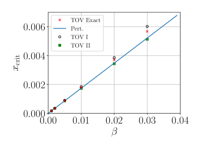
Figure 1: The dimensionless variable $x_{\rm crit}=M^{2/3}_{\rm crit}\rho^{1/3}_{0,c}$ as a function of $\beta=8k_{B}/s$ for nonrotating SMS solutions to the TOV equations. Crosses (red online) denote the numerical results for the exact treatment of the EOS from Section 3. The solid line (blue online) represents the analytical, leading-order perturbative prediction (52) from Section 3 (which is identical for Approximations I and II to the EOS). The open circles (outlined in black online) and filled squares (green online) denote the numerical results from Section 3, using Approximations I and II to the EOS, respectively. For finite entropy (nonzero $\beta$) a SMS is partially supported by gas pressure, and nonzero $x_{\rm crit}$ indicates that this stabilizes it against collapse for central densities below $\rho_{0,c}$. Compare with Fig. 1 of Paper II. As suggested in Paper II, Approximation I is indeed closer to the exact solution, despite Approximation II agreeing better with the leading-order perturbative prediction.

Figure 2: The relative change in the mass $\delta^{\rm sph}_{M}$ (see (51)) as a function of $\beta=8k_{B}/s$ for nonrotating SMS solutions. Crosses (red online) denote the numerical results using the exact EOS from Section 3. The solid and dashed lines (blue online) represent the analytical, leading-order perturbative predictions (53) and (55) derived using the energy functional method with Approximations I and II to the EOS, respectively. The open circles (outlined in black online) and filled squares (green online) denote the numerical results from Section 3. The triangles (purple online) labeled SUS represent numerical results of Shibata et al. (2016b), who adopted Approximation II. The relative change in the critical mass increases in magnitude as $\beta$ increases. As in Fig. 1, we find that Approximation I is closer to the exact treatment of the EOS than Approximation II. Compare with Fig. 2 of Paper II.

Both Fig. 1 and Fig. 2 also include perturbative results, labeled “Pert.", that are computed from analytical, leading-order perturbative expressions derived from a simple energy functional approach (see Paper II for details). Both Approximation I and II lead to identical expressions for $x_{\rm crit}$,

$$x_{{\rm crit}}=\frac{k_{2}}{4k_{4}}\beta$$ (52)

(see eqs. (49) and (56) in Paper II, hereafter (II.49) and (II.56)), where $k_{2}=0.63899$ (Lai et al., 1993) and $k_{4}=0.918294$ (Shapiro & Teukolsky, 1983). The two approximations differ, however, in their predictions for the corrections to the mass. For Approximation I, this correction is

$$\delta_{M}^{{\rm sph,I}}=\left(\frac{3}{4}\ln\frac{k_{2}}{4k_{4}}+2\ln\beta+\frac{3}{2}C\right)\beta,$$ (53)

(see (II.51)) with

$$C=\frac{k_{\tau}}{2}-\frac{1}{3}\ln\bar{M}_{0}^{\rm sph}-\frac{1}{6}\ln\eta-\frac{1}{3},$$ (54)

$k_{\tau}=-0.45928$, and $\eta$ given by (32), while for Approximation II it is

$$\delta_{M}^{{\rm sph,II}}=\left(\frac{3}{4}\ln\frac{k_{2}}{4k_{4}}+\frac{3}{4}\ln\beta-\frac{1}{2}\ln\bar{M}_{0}^{{\rm sph}}\right)\beta$$ (55)

(see (II.60)).

Fig. 1 (compare with Fig. 1 of Paper II) shows that when a SMS is partially supported by gas pressure ($\beta>0$) it is stabilized against collapse ($x_{\rm crit}>0$) for central densities below $\rho_{0,c}$. The numerical solution using the exact EOS falls between the solutions using Approximations I and II. As suggested in Paper II, Approximation I is closer to the exact solution, despite Approximation II agreeing better with the perturbative prediction.

Fig. 2 (compare with Fig. 2 of Paper II) shows that the relative change in the critical mass increases in magnitude as $\beta$ increases. As in Fig. 1, the numerical solution from handling the EOS exactly falls between the solutions using Approximations I and II, but is much closer to the results of Approximation I. Also included in this plot are numerical results of Shibata et al. (2016b), labeled SUS, who adopted Approximation II. Not surprisingly, their results agree very well with our corresponding results.

4 Rotating Supermassive Stars

As discussed in Paper I, rotation can stabilize a SMS even when it is supported by a pure radiation gas, i.e. an $n=3$ polytrope. In fact, for maximally rotating SMS, i.e. stars rotating uniformly at the mass-shedding limit, the critical configuration marking the onset of a radial instability is characterized by unique values of the dimensionless parameters

$$x_{0} \simeq 5.97\times 10^{-3},$$ (56)

$$j_{0} \simeq 0.919,$$ (57)

where $j=J/M^{2}$ is the dimensionless angular momentum, and

$$\bar{M}_{0}\simeq 4.56$$ (58)

(see Section 4.2 below). In this Section we evaluate how changes in these parameters due to the presence of gas pressure are affected by the different treatments of the gas pressure. Specifically, we will compute changes $\delta_{x}$, $\delta_{j}$ and $\delta_{M}$, defined by

$$x =x_{0}\left(1+\delta_{x}\right),$$ (59)

$$j =j_{0}\left(1+\delta_{j}\right),$$ (60)

$$\bar{M} =\bar{M}_{0}\left(1+\delta_{M}\right),$$ (61)

using the exact and approximate treatments of the gas pressure. As in Section 3 we will also compare these changes with the perturbative expressions of Paper II.

4.1 Numerical Method

We use a version of the RNS code (see Stergioulas & Friedman (1995)) slightly modified for use with SMSs. We use the tabulated EOS option with the EOSs discussed in Section 2 and tables assembled using code discussed in Section 2.4. We change the default surface values for energy density, pressure, and enthalpy in the example main.c to zero for tabulated EOSs. We also make a radial step size in the RNS code’s TOV-solver in equil.c six orders of magnitude larger. Both changes are needed because SMSs are far less dense than neutron stars, and much larger. We add a high-resolution grid option to the makefile for these calculations, increasing the number of angular gridpoints to 801 and the number of radial gridpoints to 1601. Given an EOS and a central energy density the example RNS code spins up a TOV solution until the star reaches mass-shedding, finding many intermediate configurations along the way. For a given EOS we consider many different central densities, allowing us to compute the data displayed in Figs. 3 and 4.

The curves of constant $\bar{J}$ in Figs. 3 and 4 are constructed by interpolation. Stable and unstable configurations are separated by locating the maximum mass $\bar{M}$ along curves of constant $\bar{J}$ (see Friedman et al. (1988) and discussion in Baumgarte & Shapiro (2010)). We mark these turning points in Figs. 3 and 4 with black dots. The turning point corresponding to the maximally rotating configuration is marked separately as the critical point.

4.2 Pure Radiation Fluid

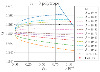
Figure 3: The mass-shedding curve (MS in the legend; solid blue online) and curves of constant $\bar{J}$ for a SMS supported by a pure radiation fluid, i.e. an $n=3$ polytrope. Black dots denote the turning points (“Turn. Pt." in the legend), i.e. maxima of curves of constant $\bar{J}$. The larger dot (red online) denotes the critical configuration (“Crit. Pt." in the legend), defined as the intersection of the turning-point and mass-shedding curves. (Compare Fig. 2 in Paper I.)

We start our analysis for a SMS supported by a pure radiation fluid, i.e. for an $n=3$ polytrope, essentially reproducing the numerical analysis of Paper I. Our results are shown in Fig. 3. In particular, we identify the critical configuration as the mass-shedding configuration at the onset of radial instability. The dimensionless parameters $x_{0}$, $j_{0}$ and $\bar{M}_{0}$ characterizing this critical configuration are given in eqs. (56) through (58) above, see also Table 1. We note that these values differ slightly from those computed in Paper I; we believe that the differences are due to the significantly higher numerical resolution used in our work here. In the following Sections we evaluate how gas pressure, treated both exactly and approximately, affects these critical parameters.

4.3 Exact Approach

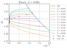
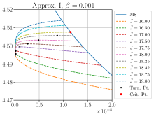
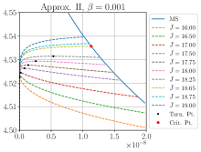
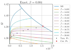
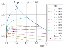
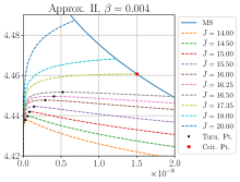
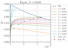
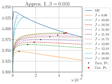
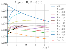
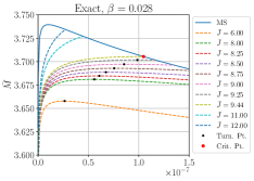
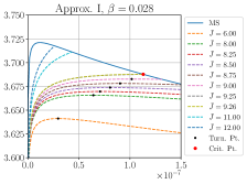
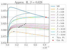
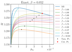
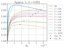
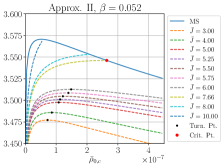
Figure 4: The mass-shedding curve (MS in each legend; blue online) and curves of constant $\bar{J}$ for different treatments of the EOS and different values of $\beta$. The left column shows results for the exact treatment of the EOS, the middle column for Approximation I, and the right column for Approximation II. Black dots mark turning points, and red dots the critical configurations, as in Fig. 3.

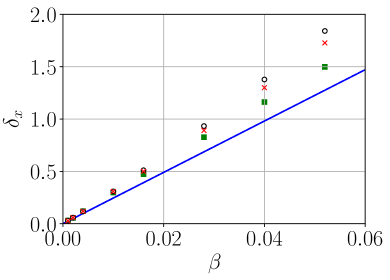
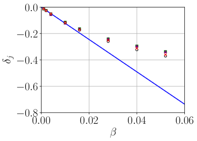
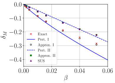
Figure 5: Effects of gas pressure on the dimensionless parameter $x$ (top left panel), the dimensionless angular momentum $j$ (top right panel), and the rescaled mass $\bar{M}$ (bottom panel) of the critical configuration of rotating SMSs. We show $\delta_{x}$, $\delta_{j}$, and $\delta_{M}$, defined in eqs. (59) – (61), as a function of $\beta$. Crosses (red online) denote numerical results from the exact treatment of the EOS. The solid and dashed lines (blue online) represent the analytical, leading-order perturbative expressions from applying the energy functional approach to Approximation I and Approximation II. The solid and dashed lines coincide for $\delta_{x}$ and $\delta_{j}$. The open circles (outlined in black online) and filled squares (green online) denote our corresponding numerical results for Approximations I and II. The triangles (purple online) in the $\delta_{j}$ and $\delta_{M}$ plots represent the numerical results of Shibata et al. (2016b), who adopted Approximation II; they agree so well with our results for Approximation II that they are difficult to distinguish in the plot. We find that Approximation I is closer to the exact treatment of the EOS than Approximation II. Compare with Fig. 3 of Paper II.

$\beta$	$R_{p}/M$	$J/M^{2}$	$\bar{M}$	$M~{}[M_{\sun}]$	$\rho_{c}~{}[{\rm g/cm^{3}}]$	$T~{}[K]$
$0$	$380$	$0.919$	$4.56$	–	–	–
$0.001$	$369$	$0.908$	$4.51$	$7.17\times 10^{7}$	$2.78\times 10^{-5}$	$1.22\times 10^{7}$
$0.002$	$358$	$0.895$	$4.46$	$1.77\times 10^{7}$	$4.96\times 10^{-4}$	$2.53\times 10^{7}$
$0.004$	$338$	$0.873$	$4.38$	$4.35\times 10^{6}$	$9.72\times 10^{-3}$	$5.39\times 10^{7}$
$0.010$	$288$	$0.811$	$4.17$	$6.64\times 10^{5}$	$0.670$	$1.61\times 10^{8}$
$0.016$	$250$	$0.762$	$4.00$	$2.48\times 10^{5}$	$7.22$	$3.02\times 10^{8}$
$0.028$	$196$	$0.688$	$3.71$	$7.51\times 10^{4}$	$158$	$6.92\times 10^{8}$
$0.040$	$159$	$0.632$	$3.47$	$3.45\times 10^{4}$	$1.35\times 10^{3}$	$1.24\times 10^{9}$
$0.052$	$133$	$0.588$	$3.27$	$1.92\times 10^{4}$	$7.25\times 10^{3}$	$1.97\times 10^{9}$

Table 1: Critical configuration parameters for an $n=3$ polytrope (first row) and for the exact treatment of the EOS (other rows). Effects of electron-positron pair production become important for temperatures greater than about $10^{9}$ K (see, e.g., Kippenhahn et al., 2012), but are ignored in our treatment here.

We start with the exact treatment of the EOS, as described in Section 2.1. To do so, we run the RNS code with the corresponding tabulated EOS for different values of $\beta=8k_{B}/s$. For each value of $\beta$ we again choose a number of different values for the central density, and let the RNS code spin the star up to mass shedding. Results from these calculations are shown in the left column of Fig. 4. We determine the critical configurations, marked by the red dots in Fig. 4, as before, and compute their physical parameters (see Table 1). Finally, we compute the corresponding changes from eqs. (59) —(61), and plot these changes in Fig. 5.

We summarize our results for critical configurations of maximally rotating SMSs partially supported by gas pressure in Figs. 6 and 7. In Fig. 6 we show the dimensionless parameters $R_{p}/M$ and $J/M^{2}$ as a function of $\beta$, as well as plotted against each other, while in Fig. 7 we show the parameters as a function of mass. For the exact treatment of the EOS we compute these physical masses by rescaling the dimensionless masses $\bar{M}$ computed in the code according to $M=K^{3/2}\bar{M}$, with $K$ given by (16).

   

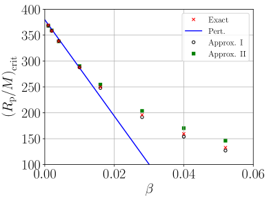
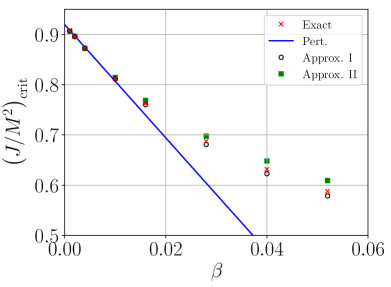
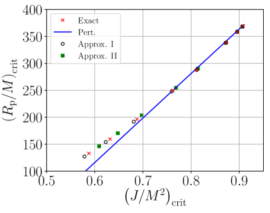
Figure 6: The dimensionless parameters $R_{p}/M$ and $J/M^{2}$ of the critical configuration, both as a function of $\beta$ (top left and top right panels) and plotted against each other (bottom panel). As expected from Fig. 5, our numerical results agree well with perturbative results for small values of $\beta$. For larger values of $\beta$, deviations between the exact treatment of the EOS and the two approximations increase as well, with Approximation I performing better than Approximation II. When plotted against each other (bottom panel), values of $R_{p}/M$ and $J/M^{2}$ appear to lie on a single line, so that deviations in radius appear to be compensated for by deviations in the angular momentum. Note, however, that, according to different approaches, individual configurations on this line correspond to different values of $\beta$.

4.4 Approximation I

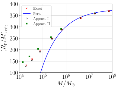
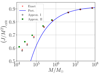
Figure 7: Same as the top two panels in Fig. 6, expect plotted against the stellar mass $M$. Compared to Fig. 6, the differences between the numerical results appear to be slightly larger in this rendering, which is caused by differences in the rescaling of the mass (see text).

For Approximation I we compute and analyze models of rotating SMS in the same way as for the exact approach, except that we now run the RNS code with EOS tables computed as discussed in Section 2.2. We show results from these calculations in the middle column of Fig. 4. We again identify the critical configurations for different values of $\beta$, compute the corresponding changes from eqs. (59) —(61), and plot these changes in Fig. 5. We also graph the parameters $R_{p}/M$ and $J/M^{2}$ in Fig. 6 and 7, where, for Approximation I, we have again computed the mass in Fig. 7 from $M=K^{3/2}\bar{M}$, with $K$ given by (16).

In Paper II we adopted a perturbative approach within a simple energy functional model to compute leading-order corrections to the critical parameters. Applying these methods for rotating SMSs and adopting Approximation I, these changes are given by

$$\delta_{j}=-\frac{1}{2}\delta{x}=-\frac{k_{1}}{8k_{3}}\frac{1}{\bar{M}_{0}^{2/3}\left(2j_{0}^{2}-j_{{\rm min}}^{2}\right)x_{0}}\beta$$ (62)

(see (II.93)) and

$$\delta_{M}^{I}=\left(\frac{3}{4}\ln x_{0}+\frac{5}{4}\ln\beta+\frac{3}{2}C+\frac{9k_{5}}{4k_{3}}\frac{x_{0}}{2j_{0}^{2}-j_{{\rm min}}^{2}}\right)\beta,$$ (63)

(see (II.96)), where $k_{3}=1.2041$ (Lai et al., 1993), and $k_{5}=0.331211$ (J. C. Lombardi Jr., 1997, priv. comm.). We also find $j_{\rm min}=0.886$ for our $n=3$ polytrope simulations. We use these expressions to calculate the perturbative curves labeled “Pert. I" in Figure 5. From $\delta_{j}$, we can compute changes in the dimensionless ratios $R_{p}/M$ and $J/M^{2}$ from

$$\left(\frac{R_{p}}{M}\right)_{\rm crit}=\left(\frac{R_{p}}{M}\right)_{\rm crit,0}\left(1+2\delta_{j}\right)$$ (64)

and

$$\left(\frac{J}{M^{2}}\right)_{\rm crit}=\left(\frac{J}{M^{2}}\right)_{\rm crit,0}\left(1+\delta_{j}\right)$$ (65)

(see (II.87) and (II.88)). These equations are plotted as the solid lines in Figs. 6 and 7, using eq. (62) and the leading-order relationship between $\beta$ and $M$

$$\beta\approx 8.46\left(\frac{M}{M_{\sun}}\right)^{-1/2}$$ (66)

(see, e.g., (II.40)).

4.5 Approximation II

Finally we repeat the same exercise with EOS tables computed from Approximation II, as discussed in Section 2.3. We show numerical results in the right column of Fig. 4. As before, critical configurations are marked by red dots. We identify the physical parameters for these critical configurations, compute changes from eqs. (59) – (61), and plot these changes in Fig. 5. As before, we also graph the polar radius and the angular momentum in Figs. 6 and 7. In the latter, we now compute the mass from $M=K_{II}^{n_{1}/2}\bar{M}$, with $K_{II}\approx(1+\beta)K$ and $n_{1}$ given by Eq. (38) (see Section 2.3).

Adopting Approximation II in the perturbative treatment of the energy functional approach leads to the same $\delta_{j}$ as Approximation I, given by (62), while $\delta_{M}$ is now given by

$$\delta_{M}^{II}=\left(\frac{3}{4}-\frac{1}{2}\ln\bar{M}_{0}+\frac{3}{4}\ln x_{0}-\frac{3}{4}\frac{j_{0}^{2}}{2j_{0}^{2}-j_{{\rm min}}^{2}}\right)\beta.$$ (67)

(see (II.105)). We use these expressions to calculate the perturbative curves labeled “Pert. II" in Fig. 5. Since expressions for $R_{p}/M$ and $J/M^{2}$ are the same in Approximation I and II, both are represented by the same perturbative line in Figs. 6 and 7.

4.6 Comparison

Figs. 5, 6, and 7 show that, for small $\beta$, corresponding to large masses, all approaches, including the perturbative treatment, lead to similar predictions for dimensionless quantities, including the dimensionless parameters $R_{p}/M$ and $J/M^{2}$ characterizing the critical configuration. In particular, our numerical results confirm our perturbative finding of Paper II that, even for masses as large as $M\simeq 10^{6}M_{\odot}$, gas pressure has a significant effect on these parameters. The reason for this behavior is the fact that, to leading order, corrections to the parameters scale with $M^{-1/2}$, and therefore decrease only slowly as the mass increases (see Eqs. (II.142) and (II.142)). For moderate values of $\beta$, or stellar masses $\lesssim 10^{6}M_{\odot}$, the analytic perturbative treatment starts to deviate from the numerical results, while both approximations implemented numerically continue to agree with each other up to larger values of $\beta$, and smaller masses. Ultimately, Approximation II in particular shows increasing deviations from the exact treatment as well.

As we had noted in Paper II, Approximation II results in predictions for changes in the mass that differ from Approximation I and the exact treatment even at leading order, both in the numerical and perturbative treatments (see the right panel in Fig. 5). We believe that at least some of these deviations may be related to the different scaling used for the different approaches: for the exact treatment and Approximation I, we rescale dimensional quantities with $K^{3/2}$ (see Eq. (16)), while for Approximation II we rescale with $K_{II}^{n_{1}/2}$. Since $K_{II}$ is only approximately constant, this approximation may well be responsible for deviations that we find in dimensional quantities.

In the left two panels of Fig. 6 we show the dimensionless parameters $R_{p}/M$ and $J/M^{2}$ as a function of $\beta$. As before, we find that, as the gas pressure becomes more important, Approximation II leads to larger deviations from the exact treatment than Approximation I. In the right panel of Fig. 6 we plot $R_{p}/M$ versus $J/M^{2}$. Remarkably, all three approaches lead to results that appear to follow a single line, even though, according to the different treatments of the gas pressure, individual configurations on this line would be identified with different values of $\beta$. Finally we graph $R_{p}/M$ and $J/M^{2}$ against stellar masses $M$ in Fig. 7. The deviations between the exact treatment of the EOS and Approximation II now appear slightly larger than in the left two panels of 7, which we attribute to the scaling of the mass, as discussed above.

5 Summary and Discussion

Recent observations of increasingly young quasars have heightened interest in the direct-collapse scenario for the formation of SMBHs, in which a SMS becomes unstable and collapses gravitationally. A number of groups have studied possible avenues for the formation of SMSs (see, e.g., Schleicher et al., 2013; Hosokawa et al., 2013; Sakurai et al., 2015; Umeda et al., 2016; Woods et al., 2017; Haemmerlé et al., 2018b, a; Wise et al., 2019, see also the discussion in Section 1). In this paper we continue the study of an idealized version of a direct-collapse scenario, involving uniformly rotating SMSs evolving along the mass-shedding limit until they reach a critical configuration marking the onset of radial instability (see Papers I and II). Identifying this critical configuration is important since it determines the dynamics of the subsequent collapse to a SMBH, including the accompanying gravitational wave signal and the properties of the remnant. In fact, many fully relativistic simulations of this collapse have adopted models of the critical configuration as initial data (see, e.g. Shapiro & Shibata, 2002; Liu et al., 2007; Montero et al., 2012; Shibata et al., 2016a; Uchida et al., 2017; Sun et al., 2019). In this paper we study the effects of gas pressure on the critical configuration. While we believe that our findings are interesting in their own right, we also hope that they will help improve future dynamical simulations of the collapse of SMSs to SMBHs.

In Paper I we found that the critical configuration is characterized by unique values of $R_{p}/M$ and $J/M^{2}$ as long as the star is dominated by radiation pressure. In Paper II we computed leading-order corrections to these values when some of the assumptions of Paper I were relaxed; in particular we considered two different approximations to estimate the effects of gas pressure. Approximation I is based on a formal expansion, while Approximation II accounts for the effects of gas pressure by simply adjusting the polytropic index in a polytropic EOS. The latter is therefore simple to implement and has been used quite commonly. Somewhat surprisingly, we found that some predictions stemming from these two approximations differed.

In this paper we apply the turning-point criterion to study more systematically the effects of gas pressure on the critical configuration of maximally rotating SMSs, and determine the critical configuration and its parameters for a large range of stellar masses. We also evaluate differences stemming from different treatments of the gas pressure. To do so, we expand on our treatment in Paper II in two ways. Instead of employing a perturbative analysis within a simple analytic energy functional model, we now compute fully relativistic numerical models of rotating SMSs. We also include a fully self-consistent, exact treatment of the EOS, in addition to the two approximations discussed above, so that we can calibrate the two approximations in the context of this idealized direct-collapse scenario.

As expected, all methods agree well for large masses, $M\gtrsim 10^{6}M_{\odot}$, corresponding to large entropies, and hence to small $\beta$ and small effects of the gas pressure. In particular, our numerical results confirm the perturbative results of Paper II that, even for these large masses, the effects of gas pressure are important. Not surprisingly, the perturbative treatment starts to deviate from the exact results first as $\beta$ increases and the mass decreases. Below $M\simeq 10^{5}M_{\odot}$, both approximations lead to increasing deviations from the exact treatment of gas pressure, but Approximation I remains much closer to the exact results than Approximation II.

References

- Agarwal et al. (2012) Agarwal B., Khochfar S., Johnson J. L., Neistein E., Dalla Vecchia C., Livio M., 2012, MNRAS, 425, 2854
- Alvarez et al. (2009) Alvarez M. A., Wise J. H., Abel T., 2009, ApJ, 701, L133
- Appenzeller & Fricke (1972) Appenzeller I., Fricke K., 1972, A&A, 21, 285
- Bañados et al. (2018) Bañados E., et al., 2018, Nature, 553, 473
- Baumgarte & Shapiro (1999a) Baumgarte T. W., Shapiro S. L., 1999a, ApJ, 526, 937
- Baumgarte & Shapiro (1999b) Baumgarte T. W., Shapiro S. L., 1999b, ApJ, 526, 941
- Baumgarte & Shapiro (2010) Baumgarte T. W., Shapiro S. L., 2010, Numerical relativity: Solving Einstein’s equations on the computer. Cambridge University Press, Cambridge
- Begelman (2010) Begelman M. C., 2010, MNRAS, 402, 673
- Begelman & Rees (1978) Begelman M. C., Rees M. J., 1978, MNRAS, 185, 847
- Begelman et al. (2006) Begelman M. C., Volonteri M., Rees M. J., 2006, MNRAS, 370, 289
- Bisnovatyi-Kogan et al. (1967) Bisnovatyi-Kogan G. S., Zel’dovich Y. B., Novikov I. D., 1967, Soviet Ast., 11, 419
- Bromm & Loeb (2003) Bromm V., Loeb A., 2003, ApJ, 596, 34
- Butler et al. (2018) Butler S. P., Lima A. R., Baumgarte T. W., Shapiro S. L., 2018, MNRAS, 477, 3694
- Chandrasekhar (1964) Chandrasekhar S., 1964, Phys. Rev. Lett., 12, 114
- Clayton (1983) Clayton D. D., 1983, Principles of Stellar Evolution and Nucleosynthesis. University of Chicago Press, http://adsabs.harvard.edu/abs/1983psen.book.....C
- Event Horizon Telescope Collaboration: K. Akiyama et al. (2019) Event Horizon Telescope Collaboration: K. Akiyama et al. 2019, ApJ, 875, L1
- Fan (2006) Fan X., 2006, New Astron. Rev., 50, 665
- Fan et al. (2006) Fan X., et al., 2006, AJ, 131, 1203
- Friedman et al. (1988) Friedman J. L., Ipser J. R., Sorkin R. D., 1988, ApJ, 325, 722
- Fuller et al. (1986) Fuller G. M., Woosley S. E., Weaver T. A., 1986, ApJ, 307, 675
- Haemmerlé et al. (2018a) Haemmerlé L., Woods T. E., Klessen R. S., Heger A., Whalen D. J., 2018a, MNRAS, 474, 2757
- Haemmerlé et al. (2018b) Haemmerlé L., Woods T. E., Klessen R. S., Heger A., Whalen D. J., 2018b, ApJ, 853, L3
- Haiman (2004) Haiman Z., 2004, ApJ, 613, 36
- Haiman (2013) Haiman Z., 2013, in Wiklind T., Mobasher B., Bromm V., eds, Astrophysics and Space Science Library Vol. 396, The First Galaxies. p. 293 (arXiv:1203.6075)
- Hosokawa et al. (2013) Hosokawa T., Yorke H. W., Inayoshi K., Omukai K., Yoshida N., 2013, ApJ, 778, 178
- Hoyle & Fowler (1963) Hoyle F., Fowler W. A., 1963, MNRAS, 125, 169
- Iben (1963) Iben Jr. I., 1963, ApJ, 138, 1090
- Johnson et al. (2013) Johnson J. L., Whalen D. J., Li H., Holz D. E., 2013, ApJ, 771, 116
- Kippenhahn et al. (2012) Kippenhahn R., Weigert A., Weiss A., 2012, Stellar Structure and Evolution, second edn. Springer
- Koushiappas et al. (2004) Koushiappas S. M., Bullock J. S., Dekel A., 2004, MNRAS, 354, 292
- Lai et al. (1993) Lai D., Rasio F. A., Shapiro S. L., 1993, ApJS, 88, 205
- Latif & Ferrara (2016) Latif M. A., Ferrara A., 2016, Publ. Astron. Soc. Australia, 33, e051
- Latif et al. (2013) Latif M. A., Schleicher D. R. G., Schmidt W., Niemeyer J., 2013, MNRAS, 433, 1607
- Liu et al. (2007) Liu Y. T., Shapiro S. L., Stephens B. C., 2007, Phys. Rev. D, 76, 084017
- Lodato & Natarajan (2006) Lodato G., Natarajan P., 2006, MNRAS, 371, 1813
- Loeb & Rasio (1994) Loeb A., Rasio F. A., 1994, ApJ, 432, 52
- Mayer et al. (2015) Mayer L., Fiacconi D., Bonoli S., Quinn T., Roškar R., Shen S., Wadsley J., 2015, ApJ, 810, 51
- Milosavljević et al. (2009) Milosavljević M., Bromm V., Couch S. M., Oh S. P., 2009, ApJ, 698, 766
- Montero et al. (2012) Montero P. J., Janka H.-T., Müller E., 2012, ApJ, 749, 37
- Mortlock et al. (2011) Mortlock D. J., et al., 2011, Nature, 474, 616
- Oh & Haiman (2002) Oh S. P., Haiman Z., 2002, ApJ, 569, 558
- Oppenheimer & Volkoff (1939) Oppenheimer J. R., Volkoff G. M., 1939, Phys. Rev., 55, 374
- Pacucci et al. (2015) Pacucci F., Volonteri M., Ferrara A., 2015, MNRAS, 452, 1922
- Press et al. (2007) Press W. H., Teukolsky S. A., Vetterling W. T., Flannery B. P., 2007, Numerical recipes in C++: The art of scientific computing, Third edition. Cambridge University Press, Cambridge
- Rees (1984) Rees M. J., 1984, ARA&A, 22, 471
- Regan & Haehnelt (2009a) Regan J. A., Haehnelt M. G., 2009a, MNRAS, 393, 858
- Regan & Haehnelt (2009b) Regan J. A., Haehnelt M. G., 2009b, MNRAS, 396, 343
- Sakurai et al. (2015) Sakurai Y., Hosokawa T., Yoshida N., Yorke H. W., 2015, MNRAS, 452, 755
- Schleicher et al. (2013) Schleicher D. R. G., Palla F., Ferrara A., Galli D., Latif M., 2013, A&A, 558, A59
- Shapiro (2004) Shapiro S. L., 2004, in Ho L. C., ed., Coevolution of Black Holes and Galaxies. Cambridge University Press, p. 103 (arXiv:astro-ph/0304202)
- Shapiro (2005) Shapiro S. L., 2005, ApJ, 620, 59
- Shapiro & Shibata (2002) Shapiro S. L., Shibata M., 2002, ApJ, 577, 904
- Shapiro & Teukolsky (1983) Shapiro S. L., Teukolsky S. A., 1983, Black Holes, White Dwarfs, and Neutron Stars: the Physics of Compact Objects. Wiley Interscience, New York, http://adsabs.harvard.edu/abs/1983bhwd.book.....S
- Shibata & Shapiro (2002) Shibata M., Shapiro S. L., 2002, ApJ, 572, L39
- Shibata et al. (2016a) Shibata M., Sekiguchi Y., Uchida H., Umeda H., 2016a, Phys. Rev. D, 94, 021501
- Shibata et al. (2016b) Shibata M., Uchida H., Sekiguchi Y.-i., 2016b, ApJ, 818, 157
- Smith et al. (2017) Smith A., Bromm V., Loeb A., 2017, Astronomy and Geophysics, 58, 3.22
- Smith et al. (2018) Smith B. D., Regan J. A., Downes T. P., Norman M. L., O’Shea B. W., Wise J. H., 2018, MNRAS, 480, 3762
- Stergioulas & Friedman (1995) Stergioulas N., Friedman J. L., 1995, ApJ, 444, 306
- Sun et al. (2017) Sun L., Paschalidis V., Ruiz M., Shapiro S. L., 2017, Phys. Rev. D, 96, 043006
- Sun et al. (2018) Sun L., Ruiz M., Shapiro S. L., 2018, Phys. Rev. D, 98, 103008
- Sun et al. (2019) Sun L., Ruiz M., Shapiro S. L., 2019, Phys. Rev. D, 99, 064057
- Tolman (1939) Tolman R. C., 1939, Physical Review, 55, 364
- Uchida et al. (2017) Uchida H., Shibata M., Yoshida T., Sekiguchi Y., Umeda H., 2017, Phys. Rev. D, 96, 083016
- Umeda et al. (2016) Umeda H., Hosokawa T., Omukai K., Yoshida N., 2016, ApJ, 830, L34
- Visbal et al. (2014) Visbal E., Haiman Z., Bryan G. L., 2014, MNRAS, 442, L100
- Wagoner (1969) Wagoner R. V., 1969, ARA&A, 7, 553
- Whalen & Fryer (2012) Whalen D. J., Fryer C. L., 2012, ApJ, 756, L19
- Wise et al. (2008) Wise J. H., Turk M. J., Abel T., 2008, ApJ, 682, 745
- Wise et al. (2019) Wise J. H., Regan J. A., O’Shea B. W., Norman M. L., Downes T. P., Xu H., 2019, Nature, 566, 85
- Woods et al. (2017) Woods T. E., Heger A., Whalen D. J., Haemmerlé L., Klessen R. S., 2017, ApJ, 842, L6
- Wu et al. (2015) Wu X.-B., et al., 2015, Nature, 518, 512
- Zeldovich & Novikov (1971) Zeldovich Y. B., Novikov I. D., 1971, Relativistic astrophysics. Vol.1: Stars and relativity. University of Chicago Press, Chicago