Electron phase-space hole transverse instability at high magnetic field

Abstract

Analytic treatment is presented of the electrostatic instability of an initially planar electron hole in a plasma of effectively infinite particle magnetization. It is shown that there is an unstable mode consisting of a rigid shift of the hole in the trapping direction. Its low frequency is determined by the real part of the force balance between the Maxwell stress arising from the tranverse wavenumber $k$ and the kinematic jetting from the hole’s acceleration. The very low growth rate arises from a delicate balance in the imaginary part of the force between the passing-particle jetting, which is destabilizing, and the resonant response of the trapped particles, which is stabilizing. Nearly universal scalings of the complex frequency and $k$ with hole depth are derived. Particle in cell simulations show that the slow-growing instabilities previously investigated as coupled hole-wave phenomena occur at the predicted frequency, but with growth rates 2 to 4 times greater than the analytic prediction. This higher rate may be caused by a reduced resonant stabilization because of numerical phase-space diffusion in the simulations.

1 Introduction

Long-lived solitary electrostatic structures that are isolated peaks of positive potential at Debye-length scale, are now routinely observed as a major high-frequency component of space-plasma turbulence [22, 7, 2, 21, 32, 1, 41, 20, 19, 39, 26, 15, 27]. They give rise to what used to be called Broadband Electrostatic Noise that occurs widely wherever unstable parallel electron distributions are present; and they are now interpreted as mostly “electron holes”: a type of nonlinear Bernstein, Greene, and Kruskal (BGK) mode [4] in which the potential is self-consistently maintained by a deficit of electron phase-space density on trapped orbits [36, 33, 6, 10]. Although electron holes are routinely produced as the endpoint of Penrose-unstable one-dimensional Vlasov-Poisson (particle-in-cell or continuum) kinetic simulations [24, 3, 10], multi-dimensional simulations observe them to be long-lived only when a magnetic field in the trapping direction suppresses “transverse instabilities” that tend to break up the electron holes [25, 23, 8, 30, 28, 31, 35, 18]. Even with a very strong magnetic field, many simulations have observed much slower growing transverse instabilities [8, 30, 29, 31, 38, 18, 42], usually associated with coupled long-parallel-wavelength potential waves, well outside the hole, that are called “streaks” or “whistlers”. These instabilities are important because they may decide the long-term fate of electron holes in the high-field regime, causing planar holes to break up into three-dimensional shapes of limited transverse extent.

This paper presents the first satisfactory theoretical analysis of transverse electron hole instability in the high-magnetic field regime. Prior analytical investigations in this regime have concentrated on coupling to the waves. The pioneering work of Newman et al. [29] correctly identified the importance of kink oscillation of the hole and calculated its real frequency in a simplified waterbag model, in agreement with simulation. The external waves are actually magnetized Langmuir oscillations at the high-frequency end of the whistler branch of the cold plasma dispersion relation at substantially oblique propagation: $\omega\simeq\omega_{p}k_{\perp}/k$ ; the other, lower frequency, end of the branch, at near-parallel propagation, is where the ionospheric whistler phenomena occur. However, Newman et al’s instability mechanism was taken to be coupling between the hole and the external waves. And their analysis inappropriately represented the hole coupling through a single long-wavelength traveling wave Fourier mode. That is not what is observed in subsequent simulations, and cannot rightly represent the localized electron hole’s effect on the wave, which gives a local impulse, a standing wave with a local step in potential, and is proportional to the hole’s acceleration, not just its displacement. Moreover the wave’s effect on the hole is not just its lowest Fourier mode. Therefore, although their simulations showed instability, their analysis was based on unjustified coupling assumptions. The other early published attempt, by Vetoulis and Oppenheim [40], at an analytic understanding of the high-field instability correctly indentified particle bounce resonance as an important ingredient, and gave an expression for the resulting electron distribution function perturbation. However it then took the perturbing potential to be a single long-wavelength mode, presumably to represent the wave, and discarded the far more important perturbation arising from the hole position shift. In other words, the particle kinetics of the hole was taken to be a small perturbation to the wave, even in the hole vicinity, rather than the wave to be a small perturbation to the hole, which is more appropriate. Berthomier et al [5], motivated by measurements of Auroral phenomena, gave a very helpful review of experiment and theory, and used a different route to solving the Vlasov-Poisson system but made essentially the same erroneous assumption that the perturbing potential was purely the wave. The shortcomings of these competing prior analyses have left the high-field instability mechanism so far unresolved, even though simulations continue to observe it. The present paper is aimed at a rigorous treatment to resolve this uncertainty.

It analyzes, for an initially planar hole, a perturbation analogous to a kink of a cylindrical plasma: a uniform shift displacement of the hole in the direction $z$ of particle trapping with a finite transverse wave-vector $k_{y}=k$, as illustrated in Fig. 1.

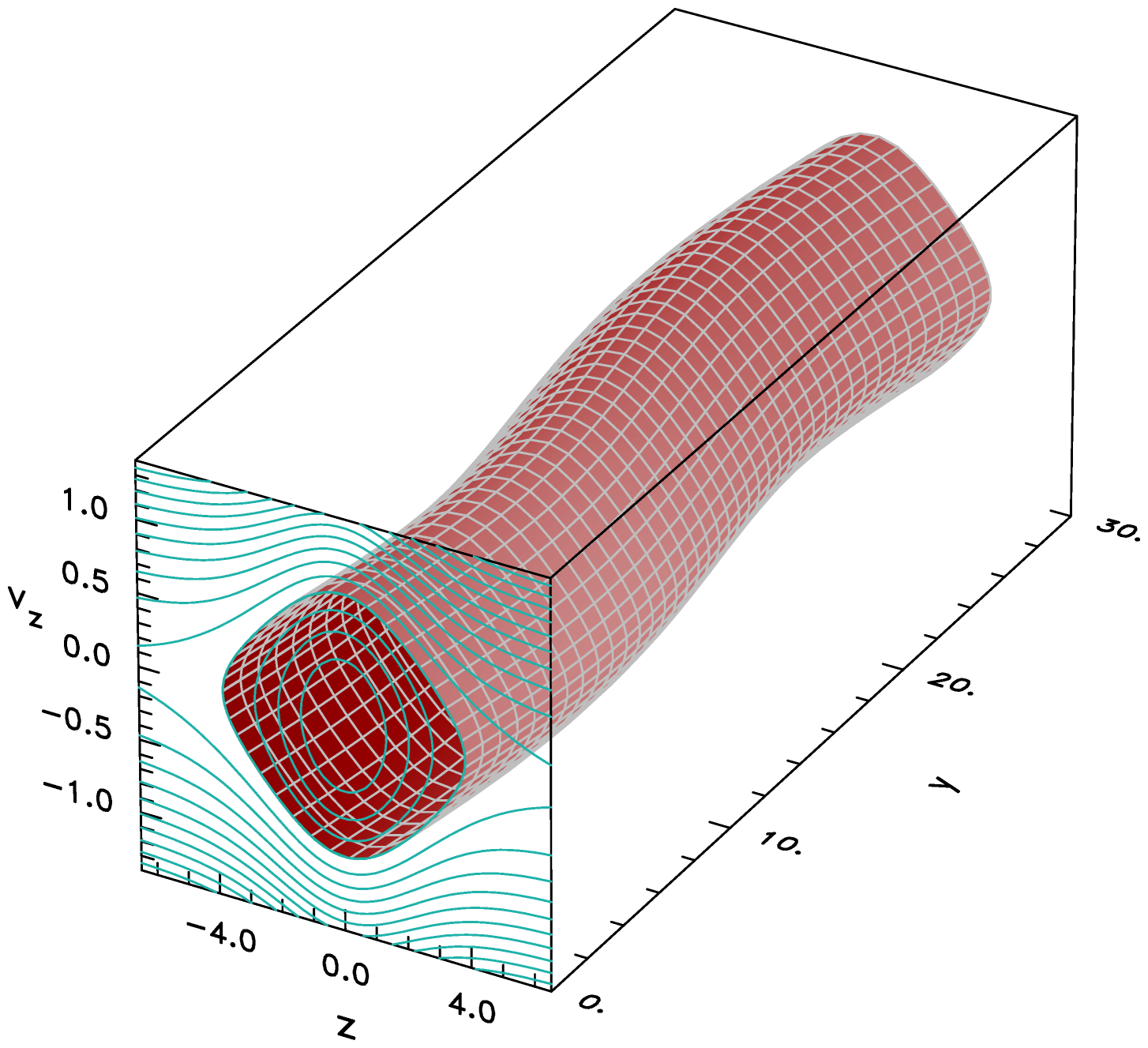
Figure 1: Illustration of the shift kink of an electron hole showing phase-space $z,v_{z}$ contours of constant energy with a specific (trapped particle) iso-energy surface rendered as a function of transverse position $y$, in three dimensions.

This eigenmode structure is adopted as an ansatz that is well theoretically justified at low frequency; and has been shown to give accurate values of real and imaginary frequencies for the transverse instability at low and moderate magnetic fields. It predicts that the low-field instability is purely growing [11, 12], that it is stabilized at a certain B-threshold [12], and is replaced by an oscillatory instability which then stabilizes above a second threshold [13], all of which are in good quantitative agreement with PIC simulations. Those simulations, however, like earlier ones, sometimes observe a residual high-magnetic field oscillatory kink instability, coupled to external waves, with a much lower growth rate. It persists to apparently arbitrarily high magnetic field (and hence cannot be attributable to cyclotron resonances [17] since its frequency shows no B-field dependence), and is the motivating observation behind the present extension of the analysis.

Suppression of transverse particle motion by the high magnetic field is a significant simplification, and allows one to derive the eigenmode equations from elementary one-dimensional understanding of the Vlasov equation, and to develop purely analytic approximations for the hole force terms whose balance gives the eigenvalue and hence the frequency and growth rate. Section 2 explains the derivation and force balance, and then provides some motivating and explanatory observations of the important physics, based on numerical orbit integration, which lays the groundwork for the analytical solution. Section 3 performs the analysis of the three dominant imaginary contributions to the particle force arising from a hole shift perturbation, using well-motivated analytic approximations of the anharmonic motion of the trapped and passing particles. Together these determine (in section 4) a universal dispersion relation between the real and imaginary parts of the frequency $\omega$ and the corresponding transverse wave-number $k$. Section 5 compares the results with some particle in cell simulations, and makes the case that the instability mechanism analysed is probably responsible for the hole-wave coupled instability observed in simulations, albeit with some caveats.

The stability analysis takes no account of any induced waves external to the hole. It shows that there is essentially always a slow-growing residual transverse instability of a slab hole at high magnetic field, regardless of the precise field magnitude, and regardless of any coupling to external waves. This instability might generate waves [34] and the simulations give evidence that it is influenced and possibly sometimes suppressed or enhanced by hole-wave coupling, but hole-wave coupling should probably be regarded as a feature, not an intrinsic causative mechanism, of the instability.

Ions are taken as a uniform immobile background, only electron dynamics are included, and the external background distribution of untrapped electrons $f_{0}$ is taken to be an unshifted Maxwellian. These simplifications well represent holes that move much faster than the ion sound speed but slower than the electron thermal speed. Throughout this paper dimensionless units are used with length normalized to Debye length $\lambda_{D}=\sqrt{\epsilon_{0}T_{e}/n_{0}e^{2}}$, velocity to electron thermal speeds $v_{t}=\sqrt{T_{e}/m_{e}}$, electric potential to thermal energy $T_{e}/e$ and frequency to plasma frequency $\omega_{p}=v_{t}/\lambda_{D}$ (time normalized to $\omega_{p}^{-1}$). In these normalized units the electron mass ($m_{e}$) is unity and is omitted from the equations but normalized electron charge is $q_{e}=-1$, and is retained. The parallel energy $W$ is written ${1\over 2}v_{z}^{2}+q_{e}\phi$.

2 High-B Instability

2.1 The Vlasov Poisson system

A rigorous analysis of the problem of transverse instability at arbitrary magnetic field strength has been presented in [12], which should be consulted for general mathematical detail. We proceed more simply here by making the early approximation of high magnetic field. A linearized analytic treatment of electrostatic instability of a magnetized electron hole depends on the first order perturbation to the distribution function $f_{1}$ caused by a potential perturbation $\phi_{1}$. It is found by integrating Vlasov’s equation along the equilibrium (zeroth order) helical orbits, which are the equation’s “characteristics”. For a collisionless situation $f$ is constant along orbits.

The integration can be expressed as an expansion in harmonics of the cyclotron frequency ($\Omega=eB/m_{e}$). However, if the magnetic field is strong enough, only the $m=0$ harmonic is important. Physically, this high-field approximation amounts to accounting only for particles’ motion along the magnetic field, and ignoring cross-field motion, taking the Larmor radius (and cross-field drifts) to be negligibly small. Vlasov’s equation is then essentially one-dimensional so we need only consider the parallel velocity distribution, denoted $f(v)$.

Because the equilibrium is non-uniform in the (trapping) $z$-direction, uncoupled Fourier representation of the potential variation is possible only for the transverse direction (taken as $y$ without loss of generality) orthogonal to $z$. The $z$-dependence of the linearized eigenmode must be expressed in a full-wave manner by writing

$$\phi_{1}({\bm{x}},t)=\hat{\phi}(z)\exp i(ky-\omega t).$$ (1)

One way to derive the solution of Vlasov’s equation intuitively is to recognize that if a small time-independent potential perturbation is applied, then particles’ (parallel) energy is still conserved as they approach from far past time (and distance). Consequently the perturbation to the distribution function ($f_{1}$) at fixed velocity arises purely as a result of the perturbation to the potential in the form $f_{1}(z)=q_{e}\phi_{1}(z){\partial f_{0}\over\partial W}$. This equation expresses the conservation of distribution function along constant energy orbits and the fact that the potential perturbation causes an orbit at fixed velocity to correspond to an energy different (in the distant past, where the distribution is $f_{0}$) by $q_{e}\phi_{1}$. This component is commonly referred to as the “adiabatic” perturbation.

However when the perturbation is time-dependent an additional effect of particle energization occurs. Particles no longer move with constant energy. Instead their energy has an instantaneous rate of increase equal to $q_{e}{\partial\phi_{1}\over\partial t}$, at every position in the past orbit. The energy change from the distant past can be written ${\cal E=}\int_{-\infty}^{t}q_{e}{\partial\over\partial t}[\phi_{1}(z(\tau),\tau)]d\tau$. The starting $f$ value (still conserved along the perturbed orbit) thus corresponds to energy smaller by ${\cal E}$. Therefore the distribution perturbation acquires a second “non-adiabatic” component $-{\cal E}{\partial f_{0}\over\partial W}$ that, for harmonic time dependence $\propto{\rm e}^{-i\omega t}$, gives a total

$$f_{1}=q_{e}\phi_{1}(t){\partial f_{0}\over\partial W}+q_{e}i\omega\Phi{\rm e}^{i(ky-\omega t)}{\partial f_{0}\over\partial W},$$ (2)

where

$$\Phi(z,t)\equiv\int_{-\infty}^{t}\hat{\phi}(z(\tau)){\rm e}^{-i\omega(\tau-t)}d\tau,$$ (3)

and $z(\tau)=z(t)+\int_{t}^{\tau}v_{z}(t^{\prime})dt^{\prime}$ is the position at earlier time $\tau$ (see [12] eq:5.6). For positive imaginary part of $\omega$ ($\omega_{i}>0$) the integral converges. We denote the second term of eq. (2) omitting the dependence ${\rm e}^{i(ky-\omega t)}$, as $\tilde{f}\equiv q_{e}i\omega\Phi\partial f_{0}/\partial W$, which is the “non-adiabatic” distribution perturbation.

The main formal difficulty is to find the shape of the eigenfunction $\hat{\phi}(z)$ which self-consistently satisfies the perturbed Poisson equation: an integro-differential eigenproblem. For slow time dependence relative to particle transit time, it can be argued on general grounds that the eigenmode consists of a spatial shift (by small distance $\xi$ independent of position) of the equilibrium potential profile ($\phi_{0}(z)$) (see [12] section 3.1) giving:

$$\hat{\phi}=-\xi{\partial\phi_{0}\over\partial z}.$$ (4)

The frequencies we care about have periods not much longer than the particle transit time, at least for particles with total energy near zero; so this shift form cannot be expected to hold exactly. However, we can obtain a good approximation to the corresponding eigenvalue of our system by expressing it in terms of a “Rayleigh Quotient”. This mathematical procedure is equivalent to requiring the conservation of total $z$-momentum under the influence of the assumed shift eigenmode. (See [12] section 3, and [16, 43]). This amounts to a “kinematic” treatment of the hole as a composite object.

The $z$-momentum balance can be derived in an elementary way by applying the zeroth and first order Poisson equations ${d^{2}\phi_{0}/dz^{2}}=-{\rho_{0}/\epsilon_{0}}$, and ${d^{2}\phi_{1}/dz^{2}}-k^{2}\phi_{1}=-{\rho_{1}/\epsilon_{0}}$ (where $\rho$ is the charge density) to the integral expression for the first order hole force $\int\rho_{0}(-d\phi_{1}/dz)dz$, using judicious integrations by parts as follows:

$$-\int\rho_{0}{d\phi_{1}\over dz}dz = \epsilon_{0}\int{d^{2}\phi_{0}\over dz^{2}}{d\phi_{1}\over dz}dz=-\epsilon_{0}\int{d\phi_{0}\over dz}{d^{2}\phi_{1}\over dz^{2}}dz$$ (5)

$$= \int{d\phi_{0}\over dz}(\rho_{1}-\epsilon_{0}k^{2}\phi_{1})dz.$$

Now, since $\rho_{0}$ is a function of $\phi_{0}$, we can also integrate by parts the other way to find

$$-\int\rho_{0}{d\phi_{1}\over dz}dz=\int{d\rho_{0}\over d\phi_{0}}{d\phi_{0}\over dz}\phi_{1}dz.$$ (6)

Combining and rearranging these expressions we get

$$F_{E}\equiv-\epsilon_{0}k^{2}\int{d\phi_{0}\over dz}\phi_{1}dz = -\int{d\phi_{0}\over dz}\left(\rho_{1}-{d\rho_{0}\over d\phi_{0}}\phi_{1}\right)dz$$ (7)

$$= -\int{d\phi_{0}\over dz}\left(\int q_{e}\tilde{f}dv_{z}\right)dz\equiv\tilde{F}.$$

The force $F_{E}$ consists of transfer by Maxwell stress in the $y$-direction of $z$-momentum ($d/dy(E_{y}E_{x}$)). It acts in a direction so as to increase the kink amplitude, in a manner analogous to a compressed spring. The force $\tilde{F}$ is exerted by the equilibrium potential on the non-adiabatic part of the charge density perturbation which is the jetting. Its real part is proportional to kink acceleration, and acts like a negative inertia. The eigenvalue equation (7) is that they must balance; we substitute into it the shift-mode form for $\phi_{1}$, eqs. (4 and 1). To lowest order, satisfying the real part of the force equation, the result is an oscillation at a real frequency whose square is proportional to the ratio of the negative tension effect and the negative inertia.

Both the real and imaginary parts of the complex momentum balance equation $F_{E}=\tilde{F}$ must be zero. But $F_{E}$ is real and positive for real $k$, and in this high-B approximation $k$ appears only in $F_{E}$ and not in $\tilde{F}$. If we regard $k$ as a free choice, then provided the sign of $\Re(\tilde{F})$ is positive, we can always satisfy $\Re(\tilde{F}-F_{E})=0$ by simply choosing the appropriate value for $k$. Consequently it is only the imaginary part $\Im(\tilde{F})$ (which is independent of $k$) that determines whether there exists a solution of the dispersion relation with a frequency $\omega=\omega_{r}+i\omega_{i}$ in the upper half plane ($\omega_{i}>0$), implying instability. We denote contributions from trapped (negative energy, $W<0$) and passing ($W>0$) particles with subscripts ‘t’ and ‘p’ respectively, and write $\tilde{F}=\tilde{F}_{t}+\tilde{F}_{p}$. At frequencies low compared with the transit time of thermal electrons across the hole, $\Re(\tilde{F}_{t})>0$, $\Re(\tilde{F}_{p})<0$, and $|\Re(\tilde{F}_{t})|>|\Re(\tilde{F}_{p})|$ so $\Re(\tilde{F})$ is indeed positive.

2.2 Numerical Evaluation Observations

A numerical implementation of the required integrations to find $\tilde{F}$ has previously been developed [12] for the specific hole equilibrium

$$\phi_{0}(z)=\psi\,{\rm sech}^{4}(z/4)$$ (8)

where the constant $\psi$ is the maximum hole potential: the “depth” of the hole. This code actually performs the integrations for arbitrary magnetic field strength but works well for the present high-B case, with some modifications, described later, newly implemented to allow accurate evaluations at $\omega_{i}\to 0$. It shows there to be unstable solutions at low frequency as illustrated by the contours of $\tilde{F}$ plotted in Fig 2. An unstable mode occurs at the intersection of the zero-contours of the real and imaginary parts of $\tilde{F}$.

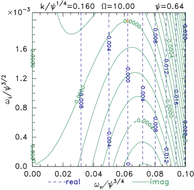
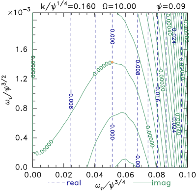
Figure 2: Contours of real and imaginary parts of $\tilde{F}-F_{E}$. Instability occurs for different $k$ at different places along the zero contour $\Im(\tilde{F}-F_{E})=0$. For the particular $k$ chosen, the eigenfrequency is show as a point.

Notice that the real part of the frequency is small even for the deep hole $\psi=0.64$, but the imaginary part is far smaller $\omega_{i}\lesssim 0.02\psi^{0.75}\omega_{r}$. The shape of the contours is approximately similar for different hole depths, when the frequencies are scaled to $\omega_{r}/\psi^{0.75}$, $\omega_{i}/\psi^{1.5}$, and the wavenumber to $k/\psi^{0.25}$. The vertical contours of real part show that there is negligible influence of $\omega_{i}$ on $\Re(\tilde{F})$ in this low frequency region. The plots are for a specific finite field $\Omega=10$, but are essentially unchanged for any $\Omega\gtrsim 5$, indicating that we are well into the high-B, one-dimensional motion, regime. We wish to derive analytically the shape of these contours in order to identify the controlling physics of this instability.

We concentrate on the decisive imaginary part of

$$\tilde{F} = -(i\omega)\xi\int q_{e}{d\phi_{0}\over dz}\int{\partial f_{0}\over\partial W}q_{e}\int_{-\infty}^{t}\hat{\phi}(z(\tau)){\rm e}^{-i\omega(\tau-t)}d\tau dvdz.$$ (9)

The resulting lowest order in $\omega$ contribution to $\tilde{F}$ is proportional to $\omega^{2}$ times a real quantity [12]. It therefore gives rise to an imaginary component $\Im(\tilde{F})=2{\omega_{i}\over\omega_{r}}\Re(\tilde{F})$. The total contribution of this type includes both trapped and passing terms but the trapped real force is typically about five times larger than the passing real force, and will be our focus in the analytic approximation. However, Fig. 2 shows there are non-zero imaginary components at $\omega_{i}\to 0$. We therefore seek, in addition, the imaginary component of the trapped particle force $\tilde{F}_{t}$ of lowest order in $\omega$ that does not depend on $\omega_{i}$. It comes from accounting to higher order for the variation of the ${\rm e}^{-i\omega(\tau-t)}$ factor, and is contributed by the resonance between the eigenfrequency $\omega$ and the bounce frequency $\omega_{b}$ of some trapped particles. There is also an important imaginary component of $\tilde{F}_{p}$ that does not depend on $\omega_{i}$.

One can exchange the order of integration in eq. (9) so as to perform the velocity integration last. The notation ${d\tilde{F}_{t}\over du}$ is used to denote the quantity that when integrated $du$ over any velocity-dependent variable $u$ gives $\tilde{F}_{t}$. Fig. 3 shows an example of the real and imaginary parts of ${d\tilde{F}_{t}\over d(-W)^{1/2}}$. The area under the curves gives the total force.

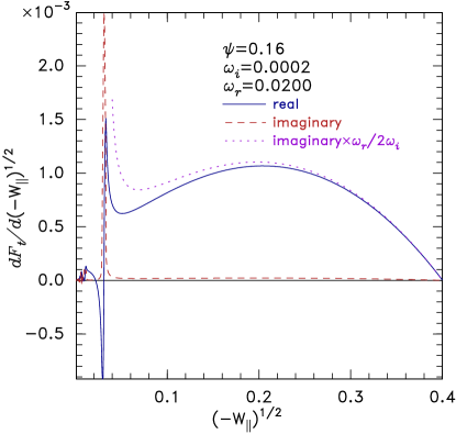
Figure 3: Example of contributions to the trapped particle force from different particle energies, showing the resonance between bounce frequency and eigenfrequency. Components: Solid line, real; dashed line, imaginary; dotted line, $\omega_{r}/2\omega_{i}\times$imaginary.

The parameter $(-W)^{1/2}$ runs from zero for the highest energy (marginally) trapped particles to $\sqrt{\psi}$ for the deepest trapped particles. As will be shown shortly, it is approximately proportional to the bounce frequency, because of the anharmonic shape of the electron hole potential $\phi_{0}$, which falls exponentially to zero in the wings. In Fig. 3 we observe for this low frequency ($\omega_{r}=0.02$, $\omega_{i}=2\times 10^{-4}$) case a resonant response at a low value of $(-W)^{1/2}$ (weakly trapped particles) corresponding to $\omega_{r}\simeq\omega_{b}$. It is obvious that in addition to the substantial real force, arising from the area under the solid curve, there is a smaller imaginary force that is dominated by the contribution from the resonance. Resonances also occur at odd harmonics of the fundamental bounce frequency of particles having lower $\omega_{b}$ that are closer to zero energy (the trapped/passing boundary). However their contribution is much smaller and can be ignored.

The low-level non-resonant imaginary contribution that extends across the entire $(-W)^{1/2}$ range in Fig. 3 arises from the component $\Im(\tilde{F})=2{\omega_{i}\over\omega_{r}}\Re(\tilde{F})$ (as is verified by the dotted line, which equals $\Re(\tilde{F})$ far from resonance). It tends to zero as $\omega_{i}\to 0$, as expected from analysis; but the narrow resonant contribution does not. Instead it becomes narrower and higher with a convergent total area. This fact poses a numerical challenge at small $\omega_{i}$ for the code that calculates $\tilde{F}$ by discrete integration. The challenge is overcome by adopting the approach made familiar in plasma physics in the context of Landau damping: namely displacing the contour of integration in the $\omega_{b}\leftrightarrow v$ plane so that it remains below the pole at $\omega_{b}=\omega$ as $\omega_{i}$ decreases toward (or even beyond) zero. Keeping the integration contour sufficiently below the pole limits the narrowness and height of the resonance, allowing it to be numerically resolved. We now obtain approximate analytic expressions for the important contributions to the imaginary force at low frequency.

3 Analytic Treatment of the Hole Momentum

3.1 Bounce Orbit Integration

First we obtain the relationship between the bounce frequency of trapped particles, $\omega_{b}$, and (unperturbed) orbit energy $W$. To approximate analytically for low frequency we observe that orbits near the separatrix ($W\to 0$) have low $\omega_{b}$ because they dwell most of their time near the turning points. The potential and its gradient are small there, and for the $\,{\rm sech}^{4}(z/4)$ hole they can be approximated as $-{d\phi_{0}\over d|z|}\simeq\phi_{0}\simeq\psi 16{\rm e}^{-|z|}$. Actually, the mechanism of Debye shielding requires, in the far wing, that $\phi_{0}\propto{\rm e}^{-|z|}$ for any hole shape that does not have infinite gradients of $f$ at the separatrix [10]. Therefore the treatment has much wider application than the specific $\,{\rm sech}^{4}$ hole-shape. In the wing (where $\phi_{0}\sim-W$) we may thus take $d\phi_{0}/\phi_{0}\simeq-d|z|$, and can write the relationship between time $t$ to pass from the turning point to a smaller $|z|$, corresponding to a larger $\phi_{0}$, as

$$t(z)=\int{-d|z|\over|v|}\simeq{1\over\sqrt{2}}\int{d\phi_{0}\over\phi_{0}\sqrt{\phi_{0}+W}}={1\over\sqrt{2}}{2\over\sqrt{-W}}\tan^{-1}\sqrt{{\phi_{0}\over(-W)}-1},$$ (10)

whose inverse is

$${\phi_{0}\over-W}=1+\tan\left(t\sqrt{-W/2}\right).$$ (11)

A quarter period of the orbit has been reached when $-\phi_{0}/W$ is large, which occurs when the value of $t\sqrt{-W/2}$ is $\simeq\pi/2$. Consequently the orbit period is approximately $t_{b}=2\pi/({\sqrt{-W/2}})$, and $\omega_{b}=\sqrt{-W/2}$.

We shall shortly also need the following average over the orbit, which can be evaluated for the first quarter period using the relation (11), initially neglecting the distinction between $\sqrt{-W/2}$ and $\omega_{b}$:

$$\left\langle{\phi_{0}\over-W}\cos\omega_{b}t\right\rangle \simeq {1\over t}\int_{0}^{t}\cos\omega_{b}t^{\prime}+\sin\omega_{b}t^{\prime}\;dt^{\prime}=[\sin\omega_{b}t-\cos\omega_{b}t+1]/\omega_{b}t.$$ (12)

Taking $\omega_{b}t=\pi/2$, we get an average equal, by symmetry, to that for a full orbit:

$$\left\langle{\phi_{0}}\sin\omega_{b}\tau^{\prime}\right\rangle=\left\langle{\phi_{0}}\cos\omega_{b}t\right\rangle\simeq{4\over\pi}(-W)\simeq{8\over\pi}\omega_{b}^{2};$$ (13)

($\tau^{\prime}$ is a shifted time, measured from the center of the orbit: $\omega_{b}\tau^{\prime}=\pi/2+\omega_{b}t$.)

Although these results are exact as $W\to 0$, and over-estimate $\omega_{b}$ by only a factor $\sqrt{2}$ at the other extreme $-W\to\psi$, their inaccuracy will turn out to be numerically significant. It arises because the estimate of $t_{b}$ has neglected the extra time it takes the orbit to pass from the place where the relationship $d\phi_{0}/\phi_{0}\simeq-d|z|$ is broken by the rounded potential peak, to the exact center of the hole $z=0$. We track the correction by writing $\omega_{b}=A\sqrt{-W/2}$ where $A$ is a correcting factor close to but slightly below unity. Approximately the same factor applies to the mapping of $W$ to $\omega_{b}^{2}$ in eq. (13) which will be written $\left\langle{\phi_{0}}\sin\omega_{b}\tau^{\prime}\right\rangle\simeq{8\over\pi}\omega_{b}^{2}/A^{2}$.

3.2 Resonant Force

To evaluate the resonant contribution of trapped particles to the force, it is convenient to integrate eq. (3) twice by parts using the fact that $\hat{\phi}=-\xi{d\phi_{0}\over dz}=\xi{dv\over d\tau}/q_{e}$:

$${q_{e}\Phi(t)\over\xi}=\int_{-\infty}^{t}{dv\over d\tau}{\rm e}^{-i\omega(\tau-t)}d\tau=v(t)+i\omega z(t)+(i\omega)^{2}\int_{-\infty}^{t}z(\tau){\rm e}^{-i\omega(\tau-t)}d\tau.$$ (14)

This is exact for an exact shift mode. If the eigenmode deviates from a shift mode (for example by having a shift $\xi$ that is a non-uniform function of $|z|$) but retains the properties of the shiftmode in that it is antisymmetric and localized to the hole, then the treatment remains valid provided we reinterpret in $\Phi$ the meaning of $v$ to be $\int q_{e}\hat{\phi}d\tau/\xi$, and $z=\int vd\tau$.

The benefit of this reexpression is that, measuring $\tau$ from where $z=0$, $z(\tau)$ is an approximate square-wave in time on low bounce frequency orbits. Also, when we integrate the resulting $\tilde{f}{d\phi_{0}\over dz}$ over the hole extent, to obtain $\tilde{F}_{t}$, the antisymmetry of ${d\phi_{0}\over dz}$ annihilates any symmetric part of $\tilde{f}$ and hence of $\Phi$. Therefore the term $v(t)$ can be dropped. Choose the zero of $\tau$ and $t$ to be where $v$ is positive, during the bounce period chosen to minimize $|t|$. Then the integral in eq. (14) can be separated into two parts: $\int_{0}^{t}$ with $|t|\leq t_{b}/2$ plus $\int_{-\infty}^{0}$. Only $\int_{-\infty}^{0}$ contributes to the resonant term. The other (non-resonant) terms will be dealt with later.

Represent the square-wave during the final orbit as $z(t)=sign(t)z_{A}$. The resonant part of the integral may then be evaluated as

$${q_{e}\Phi_{R}\over(i\omega)^{2}\xi} = \int_{-\infty}^{0}z(\tau){\rm e}^{-i\omega(\tau-t)}d\tau={1\over 1-{\rm e}^{i\omega t_{b}}}\int_{-t_{b}}^{0}z(\tau){\rm e}^{-i\omega(\tau-t)}d\tau$$

$$= {z_{A}{\rm e}^{i\omega t}\over 1-{\rm e}^{i\omega t_{b}}}{1\over i\omega}\left(\left[{\rm e}^{-i\omega\tau}\right]_{-t_{b}/2}^{0}-\left[{\rm e}^{-i\omega\tau}\right]_{-t_{b}}^{-t_{b}/2}\right)$$

$$= {z_{A}{\rm e}^{i\omega t}\over i\omega}{\left(1-{\rm e}^{i\omega t_{b}/2}\right)^{2}\over 1-{\rm e}^{i\omega t_{b}}}={z_{A}{\rm e}^{i\omega t}\over i\omega}{1-{\rm e}^{i\omega t_{b}/2}\over 1+{\rm e}^{i\omega t_{b}/2}}\left[={z_{A}{\rm e}^{i\omega t}\over\omega}\tan(\omega t_{b}/4)\right].$$

The denominator $1+{\rm e}^{i\omega t_{b}/2}$ becomes zero, giving resonances, when $\omega t_{b}=2\pi\ell$ with $\ell$ an odd integer. In the vicinity of the $\ell$th (odd) resonance

$${1-{\rm e}^{i\omega t_{b}/2}\over 1+{\rm e}^{i\omega t_{b}/2}}\simeq{2\over 1-{\rm e}^{i\pi(\omega-\ell\omega_{b})/\omega_{b}}}\simeq{-2\omega_{b}\over i\pi(\omega-\ell\omega_{b})}.$$ (16)

Thus at resonance

$$\tilde{f}_{R}=q_{e}i\omega\Phi_{R}{\partial f_{0}\over\partial W}\simeq-\xi{\partial f_{0}\over\partial W}{z_{A}{\rm e}^{i\omega t}}{(i\omega)^{2}2\omega_{b}\over i\pi(\omega-\ell\omega_{b})},$$ (17)

in which $t$ represents the end point $z(t)$ (zero when $t=0$) of the orbit: the position where $\tilde{f}$ is being evaluated. Also, in general, for small positive imaginary part $\omega_{i}$, the integral through (strictly close under) a resonance is

$$\int_{-}^{+}{g(\omega_{b})\over(\ell\omega_{b}-\omega_{r}-i\omega_{i})}d\omega_{b}\simeq{i\pi\over\ell}g(\omega_{r}/\ell)$$ (18)

for any slowly varying function $g$.

We now need to get the total non-adiabatic force by integrating $-q_{e}{d\phi_{0}\over dz}\tilde{f}_{R}$ over the relevant phase space $dz\,dv$. Our current interest is the trapped particles, which occupy a finite area of phase space bounded by the separatrix. The best way to carry out this area integral is not along fixed values of $v$ or $z$, but along fixed values of energy, following the orbits along which particles move as a function of time (denoted $\tau^{\prime}$). It is convenient to represent the orbit energy by the value of the velocity at the hole center $z=0$ where the potential has its single maximum, $\psi$, because every orbit does in fact pass through this position. We write this velocity $v_{\psi}$ (taken positive) so that (the negative quantity) $W=q_{e}\psi+{1\over 2}v_{\psi}^{2}=q_{e}\phi(z)+{1\over 2}v(z)^{2}$. Then, since at constant energy $vdv=v_{\psi}dv_{\psi}$, we have $dz\,dv\to vd\tau^{\prime}\,dv=d\tau^{\prime}v_{\psi}dv_{\psi}=d\tau^{\prime}dW\simeq-d\tau^{\prime}4\omega_{b}d\omega_{b}/A^{2}$ (using $\omega_{b}^{2}=-A^{2}W/2$). Incidentally, the numerical integration code is implemented in the same way, but it uses none of the present approximations.

The resonant force as $\omega_{i}\to 0$ can then be written, using first the parity relations, and then eqs. (17), (18), and (13), as

$$\tilde{F}_{R} = -q_{e}\int_{0}^{\sqrt{-2q_{e}\psi}}\int_{-t_{b}/2}^{t_{b}/2}{d\phi_{0}\over dz}\tilde{f}_{R}(\tau^{\prime})d\tau^{\prime}v_{\psi}dv_{\psi}$$ (19)

$$\simeq -q_{e}\int_{0}^{\sqrt{-2q_{e}\psi}}\int_{0}^{t_{b}/2}{d\phi_{0}\over d|z|}[\tilde{f}_{R}(\tau^{\prime})-\tilde{f}_{R}(-\tau^{\prime})]d\tau^{\prime}v_{\psi}dv_{\psi}$$

$$\simeq -q_{e}\xi\int^{0}_{\sqrt{\psi}/2}{\partial f_{0}\over\partial W}{(i\omega)^{2}z_{A}2\omega_{b}\over i\pi(\omega-\ell\omega_{b})}\int_{0}^{t_{b}/2}\phi_{0}2i\sin(\omega\tau^{\prime})d\tau^{\prime}4\omega_{b}d\omega_{b}/A^{2}$$

$$\simeq q_{e}\xi\int^{\sqrt{\psi}/2}_{0}{\partial f_{0}\over\partial W}{(i\omega)^{2}z_{A}2\omega_{b}\over i\pi(\omega-\ell\omega_{b})}i\left\langle\phi_{0}\sin(\omega\tau^{\prime})\right\rangle t_{b}4\omega_{b}d\omega_{b}/A^{2}$$

$$\simeq q_{e}\xi\left.{\partial f_{0}\over\partial W}\right|_{R}(i\omega_{r})^{2}z_{A}{2\omega_{R}\over\ell}{i}\left\langle\phi_{0}\cos(\omega_{r}t)\right\rangle 8\pi/A^{2}$$

$$\simeq -iq_{e}\xi z_{A}\left.{\partial f_{0}\over\partial W}\right|_{R}128\omega_{R}^{5}/A^{4},\qquad{\rm for}\ \ell=1.$$

where $\omega_{R}=\omega_{r}/\ell$ is the resonant bounce frequency. This surprisingly simple expression has not to my knowledge been previously discovered.

It should be remarked that eq. (19) has no explicit dependence on the hole depth $\psi$. However, the (positive) value of ${\partial f_{0}\over\partial W}$ varies generally as $\sim\psi^{-1/2}$ [14, 10]; more specifically, for a $\,{\rm sech}^{4}(z/4)$ hole it can be shown analytically that

$$f_{0} = f_{0s}\left[{2\over\sqrt{\pi}}\sqrt{-W}+{15\over 16}\sqrt{\pi\over\psi}W+\exp(-W){\rm erfc}(\sqrt{-W})\right],$$ (20)

$${\partial f_{0}\over\partial W} = f_{0s}\left[{15\over 16}\sqrt{\pi\over\psi}-\exp(-W){\rm erfc}(\sqrt{-W})\right],$$ (21)

where $f_{0s}$ is the distribution function at the separatrix ($W=0$, $\exp(0){\rm erfc}(0)=1$), and for unit density $f_{0s}=1/\sqrt{2\pi}$. We will write this ${\partial f_{0}\over\partial W}\simeq D(15/16)/\sqrt{2\psi}$, where $D$ is a correction factor approximately equal to $1-(16/15)\sqrt{\psi/\pi}$, somewhat smaller than unity. For a general (non-shift) antisymmetric potential perturbation $\hat{\phi}$ one should take $\xi z_{A}=-\int\int\hat{\phi}(\tau^{\prime})d\tau^{\prime}d\tau$, in accordance with the remarks following eq. (14). The fifth power dependence upon $\omega_{R}$ is one guarantee that $\ell=3$ and higher harmonic resonances can be ignored. So, henceforth we consider only $\ell=1$. For small frequencies $\omega_{R}$, the turning point position $z_{A}$ is approximately equal to the half-width of the hole, and varies only logarithmically at low frequency, because it occurs at $2\omega_{R}^{2}=-W=\phi_{0}(z)\simeq 16\psi{\rm e}^{-|z|}$ in the wings, so for an exact shift mode

$$z_{A}\simeq\ln\left(16\psi\over 2\omega_{R}^{2}\right)=\ln\left(8\psi^{-1/2}\over(\omega_{R}^{2}/\psi^{3/2})\right)\simeq\ln\left(8\psi^{-1/2}\over(0.05)^{2}\right)=8.-\ln(\psi)/2,$$ (22)

using the observed numerical scaling $\omega_{r}/\psi^{3/4}\sim 0.05$. The value $z_{A}=9$ will be used as a generic estimate. The dominant dependency is $\tilde{F}_{R}\propto\xi\omega_{r}^{5}/\psi^{1/2}$, and we will ignore the weak dependence on $\psi$ and $\omega_{r}$ of $z_{A}$ and of the correction factors $D$ and $A$, in estimating the constant of proportionality. For $\psi=0.16$, $D=0.76$, and $A$ can be as small as $0.9$, in which case $D/A^{4}\simeq 1.15$ and the combined correction factors are moderate giving $\tilde{F}_{R}\simeq 1000i\xi\omega_{r}^{5}/\sqrt{\psi}$.

3.3 Non-resonant Force

The non-resonant contribution to eq. (14) is the sum of the non-resonant ($\int_{0}^{t}$) integral plus the term $i\omega z(t)$. If treated using the square-wave approximation $z(t)=sign(t)z_{A}$ it is

$${q_{e}\Phi_{NR}(t)\over i\omega\xi}=z(t)+(i\omega)\int_{0}^{t}z(\tau){\rm e}^{-i\omega(\tau-t)}d\tau=sign(t)z_{A}{\rm e}^{i\omega t},$$ (23)

taking into account that the signs of $z$ and $t$ are the same. When multiplied by the antisymmetric quantity $-(i\omega)^{2}q_{e}{d\phi_{0}\over dz}$ and integrated for positive and negative $z(t)$ and $v$ this gives rise to a force

$$\tilde{F}_{NR}=-(i\omega)^{2}\xi\int_{0}^{\sqrt{-2q_{e}\psi}}{\partial f_{0}\over\partial W}\int_{0}^{t_{b}/2}z_{A}2\cos\omega\tau^{\prime}q_{e}{d\phi_{0}\over dz}d\tau^{\prime}v_{\psi}dv_{\psi}.$$ (24)

This expression is manifestly real when $\omega_{i}=0$, and provides the main contribution to $\Re(\tilde{F}_{t})$. But it also makes an important contribution, first order in $\omega_{i}$, to $\Im(\tilde{F}_{t})$: approximately $(2\omega_{i}/\omega_{r})\tilde{F}_{NR}(\omega_{r})$.

It is less clear for the non-resonant contribution that the square-wave approximation to $z(t)$ is accurate, since contributions to this integral also arise from deeply trapped particles, which have almost sinusoidal bounce motion. Nevertheless, proceeding as before to replace $-q_{e}{d\phi_{0}\over dz}={dv\over d\tau^{\prime}}$, we get $-\int_{0}^{t_{b}/2}\cos\omega\tau^{\prime}q_{e}{d\phi\over dz}d\tau^{\prime}=\int_{0}^{t_{b}/2}\cos\omega\tau^{\prime}{dv\over d\tau^{\prime}}d\tau^{\prime}=-v_{\psi}+v(t_{b}/2)\cos(\omega t_{b}/2)+\int\omega\sin\omega\tau^{\prime}v(\tau^{\prime})d\tau^{\prime}$. The final integral term can be ignored by $\omega$ ordering and the second because $v(t_{b}/2)=0$ everywhere except on a negligible measure at $\omega t_{b}/2\simeq n\pi$; so we can substitute $-v_{\psi}$ for $-\int_{0}^{t_{b}/2}\cos\omega\tau^{\prime}q_{e}{d\phi\over dz}d\tau^{\prime}$, giving

$$\tilde{F}_{NR} \simeq -(i\omega)^{2}\xi\int_{0}^{\sqrt{-2q_{e}\psi}}{\partial f_{0}\over\partial W}z_{A}2v_{\psi}v_{\psi}dv_{\psi}$$ (25)

$$\simeq -(i\omega)^{2}\xi\left\langle{\partial f_{0}\over\partial W}2z_{A}\right\rangle{1\over 3}(2\psi)^{3/2}=\omega^{2}\xi w_{t}f_{0s}\sqrt{2\pi}{5\over 8}\psi,$$

where $\left\langle{\partial f_{0}\over\partial W}2z_{A}\right\rangle$ denotes an average over energy whose weighting $\propto v_{\psi}^{2}$ (emphasizing shallowly trapped orbits) justifies writing it as $w_{t}f_{0s}(15/16)\sqrt{\pi/\psi}$, with $w_{t}\sim 2z_{A}$ a hole width somewhat greater than unity. [But the $z_{A}$ here is not just for resonant orbits; it is an average over all trapped particles.] This expression for unit density is ${5\over 8}w_{t}\omega^{2}\xi\psi=5\omega^{2}\xi\psi$ when $w_{t}=8$ which is a plausible estimate.

The non-resonant $\omega_{i}$-term involves in addition a small contribution from passing particles. The total value $\Re(\tilde{F}/\omega^{2})$ has been evaluated more precisely elsewhere [16, 12], and for unit density can be written in terms of the function $h(\chi)=-{2\over\sqrt{\pi}}\chi+(2\chi^{2}-1){\rm e}^{\chi^{2}}{\rm erfc}(\chi)+1=\chi^{2}-{2\over\sqrt{\pi}}{4\over 3}\chi^{3}+O(\chi^{4}),$ where $\chi^{2}=\phi_{0}(z)$, as

$$\tilde{F}_{NR}=\xi\omega^{2}\int h(\sqrt{\phi_{0}(z)})dz=\xi\omega^{2}\psi w_{i}\simeq\xi\omega^{2}\int\phi_{0}(z)dz,$$ (26)

which can be considered to define a width $w_{i}\simeq\int\phi_{0}dz/\psi$. For shallow holes of the chosen shape, it is $w_{i}\simeq\int\,{\rm sech}^{4}(z/4)dz=16/3$, giving $\tilde{F}\simeq 5.3\xi\omega^{2}\psi$, in excellent agreement with the estimate developed from eq. (25), confirming that the passing particle contribution is relatively unimportant here.

3.4 Passing-Particle Imaginary Force

To obtain the lowest order imaginary part of the passing-particle force that is independent of $\omega_{i}$ we proceed in a similar manner using two integrations by parts, except with different constants of integration than eq. (14).

$${q_{e}\Phi(t)\over\xi}=[v(t)-v_{\infty}]+i\omega[z(t)-z_{\infty}(t)]+(i\omega)^{2}\int_{-\infty}^{t}[z(\tau)-z_{\infty}(\tau)]{\rm e}^{-i\omega(\tau-t)}d\tau.$$ (27)

Here $v_{\infty}$ denotes the distant velocity (outside the hole) of the orbit under consideration; and $z_{\infty}(t)=v_{\infty}t+const.$ denotes the position as a function of time for motion at a constant velocity $v_{\infty}$ which extrapolates the distant past orbit ignoring $\phi(z)$. Thus $[z(\tau)-z_{\infty}(\tau)]$ is zero in the distant past, rises as it passes through the hole, and then remains constant past the hole. As before, it is the final integral term that gives the imaginary force (real part of $\Phi$). We approximate the integral by treating $[z(\tau)-z_{\infty}(\tau)]$ as the unit step function $H(\tau)\equiv[1+sign(\tau)]/2$ times an amplitude $z_{p}=\int_{-\infty}^{\infty}[v(t)-v_{\infty}]dt$, and note that $\int_{-\infty}^{t}H(\tau){\rm e}^{-i\omega(\tau-t)}d\tau=H(t)[1-{\rm e}^{i\omega t}]/(-i\omega)$. Then, ignoring other terms that are subsequently annihilated by symmetry, we have for small $\omega t$ a term independent of $\omega_{i}$

$$\Re\{q_{e}\Phi(t)\}\simeq\Re\{(-i\omega)\xi z_{p}[1-{\rm e}^{i\omega t}]H(t)\}\simeq(i\omega_{r})^{2}\xi z_{p}tH(t).$$ (28)

From the second term of eq. (27) we also have a component of $q_{e}\Phi(t)$ equal to $i\omega_{r}z_{p}H(t)$, which could be pursued, but it contributes imaginary force only $\propto\omega_{i}$ and is subdominant to the similar trapped component, so we do not bother. The required imaginary contribution to passing force at $\omega_{i}=0$ is thus

$$i\Im(\tilde{F}_{p}) \simeq -\int\int q_{e}{d\phi_{0}\over dz}\xi(i\omega)^{3}{\partial f_{0}\over\partial W}z_{p}\tau^{\prime}H(\tau^{\prime})d\tau^{\prime}v_{\infty}dv_{\infty}$$ (29)

$$= -q_{e}\xi(i\omega)^{3}\int{\partial f_{0}\over\partial W}z_{p}\int_{0}^{\infty}-\tau^{\prime}{dv\over d\tau^{\prime}}d\tau^{\prime}v_{\infty}dv_{\infty}$$

$$= -q_{e}\xi(i\omega)^{3}\int{\partial f_{0}\over\partial W}z_{p}\int_{0}^{\infty}[v(\tau^{\prime})-v_{\infty}]d\tau^{\prime}v_{\infty}dv_{\infty}$$

$$= -q_{e}\xi(i\omega)^{3}\int{\partial f_{0}\over\partial W}{z_{p}^{2}\over 2}v_{\infty}dv_{\infty}.$$

The integral quantity $z_{p}(v_{\infty})=\int(1-|v_{\infty}/v|)dz$ is approximately the value of its integrand at the hole center times the hole width: $z_{p}(v_{\infty})\simeq(1-v_{\infty}/\sqrt{v_{\infty}^{2}+2\psi})w_{p}$. Its dependence for $v_{\infty}^{2}\gtrsim\psi$ is $z_{p}\simeq w_{p}\psi/v_{\infty}^{2}$; so $\int_{\psi}^{\infty}z_{p}^{2}dv_{\infty}^{2}\simeq w_{p}^{2}\psi$, and for small $\psi$ we can multiply this by the value of $df_{0}/dW$ at small energy. The remainder of the integral can be approximated as having constant $z_{p}\simeq w_{p}$ so $\int_{0}^{\psi}z_{p}^{2}dv_{\infty}^{2}\simeq w_{p}^{2}\psi$, giving

$$\int_{0}^{\infty}{\partial f_{0}\over\partial W}{z_{p}^{2}\over 4}dv_{\infty}^{2}\simeq\left.{\partial f_{0}\over\partial W}\right|_{v_{\infty}=0}w_{p}^{2}{\psi\over 2}$$ (30)

(which can be considered the definition of $w_{p}$). Thus finally

$$\Im(\tilde{F}_{p})\simeq q_{e}\xi\omega^{3}\left.\partial f_{0}\over\partial W\right|_{0}{w_{p}^{2}\over 2}\psi.$$ (31)

This is negative because $\left.\partial f_{0}\over\partial W\right|_{0}=-f_{0s}=-1/\sqrt{2\pi}$ for unit density. Also notice that despite depending on ${\partial f_{0}\over\partial W}$ this is not a resonance effect but is contributed by all energies from zero to a few times $\psi$.

4 Solution of the Dispersion Relation

4.1 Complex Frequency

We now have analytic approximations of the three terms that at low frequency predominate the relation that the total imaginary part of the hole force must vanish:

$$2{\omega_{i}\over\omega_{r}}\Re(\tilde{F})+\Im(\tilde{F}_{t})+\Im(\tilde{F}_{p})=\xi[C_{i}\omega_{i}\omega_{r}\psi+C_{t}\psi^{-1/2}\omega_{r}^{5}+C_{p}\omega_{r}^{3}\psi]=0.$$ (32)

Here the primary $\omega$ and $\psi$ dependences have been written explicitly, leaving coefficients $C_{i}\simeq 10$, $C_{t}\simeq 1000$, and $C_{p}\simeq-w_{p}^{2}/2\sqrt{2\pi}\simeq-7$ (for $w_{p}=6$, a plausible value chosen with hindsight) for unit density $f_{0s}=1/\sqrt{2\pi}$ that are approximately constant. Writing $\hat{\omega}_{r}=\omega_{r}/\psi^{3/4}$ and $\hat{\omega}_{i}=\omega_{i}/\psi^{3/2}$ the relation becomes

$$0=\Im(\tilde{F})=\xi\psi^{13/4}\hat{\omega}_{r}[C_{i}\hat{\omega}_{i}+C_{t}\hat{\omega}_{r}^{4}+C_{p}\hat{\omega}_{r}^{2}]$$ (33)

which demonstrates the universality (observed approximately in Fig.2) when expressed in the scaled quantites $\hat{\omega}_{r}$ and $\hat{\omega}_{i}$. It also reproduces the quantitative results of Fig. 2, and specifically the zero contour of $\Im(\tilde{F})$.

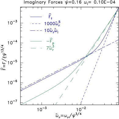
(a)  (b)

Figure 4: (a) Numerical integration (solid lines) agrees asymptotically with the analytic approximations (dashed lines) of the three terms in the imaginary force. The curve is universal when expressed in scaled quantities $\hat{\omega}_{r}$, $\hat{\omega}_{i}$ and $\hat{F}$. (b) The contours of force resulting from the analytic expressions, showing good shape agreement with Fig 2.

First though, Fig. 4(a) demonstrates the agreement of the analytic formulas for the three imaginary components of the force with the corresponding parts of the force calculated by the numerical integration code. All the forces in that plot are normalized in the form $\hat{F}\equiv\tilde{F}/\xi\psi^{13/4}$, in accordance with eq. (33), giving an essentially universal plot, independent of $\psi$ (when small) expressed in terms of $\hat{\omega}$. The agreement of the analytic curves with the appropriate range of the full numerical integration is very good, confirming that the dominant terms (of 32) have been correctly indentified and quantitatively estimated.

Fig. 4(b) shows the shape of the force contours for comparison with Fig. 2. The agreement is within the level of variation expected. The position of the bottom right-hand end of the zero contour, at $\omega_{i}=0$, is decided by setting equal and opposite the second and third terms, whose solution can be rendered as

$$\hat{\omega}_{r}=\sqrt{-C_{p}/C_{t}}\simeq\sqrt{7/1000}=0.084.$$ (34)

Near the bottom left hand end we can neglect the trapped term and find

$$\hat{\omega}_{i}\simeq(-C_{p}/C_{i})\hat{\omega}_{r}^{2}\simeq 0.7\hat{\omega}_{r}^{2}.$$ (35)

This parabolic $\hat{\omega}_{r}$-dependence appears to be present in Fig. 2 (though numerical rounding and other uncertainties make the zero contour shape imprecise) and is obvious in Fig. 4(b). The top of the contour is determined by maximizing $-C_{t}\hat{\omega}_{r}^{4}-C_{p}\hat{\omega}_{r}^{2}$ which gives

$$\hat{\omega}_{r}=\sqrt{-C_{p}\over 2C_{t}}\simeq 0.06$$ (36)

and then

$$\hat{\omega}_{i}={1\over 2}\left(-C_{p}\over C_{i}\right)\omega_{r}^{2}={1\over 4}\left(-C_{p}\over C_{i}\right)\left(-C_{p}\over C_{t}\right)\simeq 1.2\times 10^{-3}.$$ (37)

These expressions agree with the corresponding positions on the zero contour in Fig. 4(b) (as they must).

It is clear from these observations that the effect of the resonant force is to limit the maximum $\omega_{r}$ at which instability can occur. In other words, it is a stabilizing term (contradicting Refs. [29, 40, 5]), which as $\omega_{r}$ increases eventually overcomes the others because it varies as a higher power. If its coefficient $C_{t}$ were reduced, for example by decreasing the distribution gradient ${\partial f_{0}\over\partial W}$ for shallowly trapped particles, or for a perturbation whose shift was smaller in the wings of the hole, the effect would be to permit instability to higher $\omega_{r}$ and with higher $\omega_{i}$, following the $\hat{\omega}_{i}\simeq 0.35\hat{\omega}_{r}^{2}$ trajectory further up. The stabilizing nature of the resonance might appear counter-intuitive since ${\partial f_{0}\over\partial W}$ is positive causing resonant particles to give energy to the eigenmode. What makes this effect stabilizing, however, is that the eigenmode is a “negative energy” mode, reflecting the negative inertia of the hole. Therefore adding energy to it tends to reduce its amplitude.

4.2 Wavenumber

As explained earlier, the wavenumber must be chosen to satisfy the real part of eq. (7) $\Re(\tilde{F})=F_{E}$. The real frequency $\omega_{r}$ gives the predominant real part of $\tilde{F}$ at low frequency, namely $\Re(\tilde{F})=(C_{i}/2)\xi\omega_{r}^{2}\psi$, see eqs. (26) and (32). The Maxwell stress force can be evaluated in dimensionless units as

$$F_{E}=\xi k^{2}\int\left(d\phi_{0}\over dz\right)^{2}dz={128\over 315}\xi k^{2}\psi^{2},$$ (38)

from which we conclude

$$k^{2}={315\over 128}{C_{i}\over 2}{\omega_{r}^{2}\over\psi},\qquad{\rm giving}\quad\hat{k}={k\over\psi^{1/4}}=\sqrt{315C_{i}\over 256}\hat{\omega}_{r}=3.5\hat{\omega}_{r}.$$ (39)

At the maximum unstable $\omega_{i}$, $\hat{\omega}_{r}\simeq 0.06$, we then require $\hat{k}\simeq 0.2$, which is in reasonable agreement with Fig. 2. We have recovered the observed scaling of the universal solution: $k=\hat{k}\psi^{1/4}$, and approximately the absolute value of $\hat{k}$ required for maximum instability growth.

5 Comparison with simulation

The high-B ($\Omega>2\omega_{p}$) instability investigated here was first observed in particle in cell simulations of initially uniform two-stream electron distributions [8, 30, 31], and has been observed in similar simulations since [38, 18, 37]. The electron holes form from non-linear Langmuir instability and then usually experience transverse instabilities coupled to external waves. Umeda et al [38] observed that warm beams with significant velocity spread give shallower holes, and they found no transverse hole instability for depth $\psi\lesssim 0.8$ at high-B. Such treatments may well be appropriate for a full scale simulation of events of nature, but for insight into the instability mechanisms, they suffer from difficulties associated with the highly distorted and uncertain electron velocity distributions and a high level of fluctuations associated with different wave phenomena.

Single holes deliberately set up by initial simulation conditions have been studied as an alternative that provides cleaner insight in the linear instability growth. Oppenheim et al [30] generated slab holes from (effectively) one-dimensional two-stream simulations, which were then used as initial conditions for a two-dimensional PIC simulation. It is not clear what the distribution function $f_{0}$ actually was when multidimensional dynamics was turned on. Publications observing high-B hole-wave instability of pre-formed holes of specified distribution seem to be limited to the continuum Vlasov simulation of deep waterbag holes by Newman et al [29] and the PIC simulations of Wu et al [42] ($\psi=0.8,2$). A waterbag distribution, for which $\partial f_{0}/\partial W=0$, unfortunately makes zero (or, at the waterbag boundary, infinite) the crucial resonant term. Wu’s potential profiles were Gaussian, corresponding still to rather pathological electron velocity distributions with infinite gradient at the separatrix; and they documented mostly the nonlinear phases.

Therefore new simulations have been run to compare with the present theory. They use the COPTIC particle in cell code [9], pushing only electrons (typically $\sim 1$ billion, on 512 processors) on a 2-D rectangular periodic domain with mesh spacing 1 (Debyelength) and timestep 0.5. They have effectively infinite magnetization. A hole of specified depth $\psi$ is created at the center $z=0$ by prescribing the initial particle distribution solved for by the integral equation BGK method, and loaded using a quiet-start particle placement. The initial hole has a modified potential form $\phi=\psi[1+\exp(1/\psi)]/[1+\exp(1/\psi)\cosh^{4}z/4]$ which has a stretched potential top unless $\psi$ is rather small. This modification recognizes that an exact $\,{\rm sech}^{4}z/4$ hole cannot exist for $\psi>0.75$ because it requires a negative central distribution function $f_{0}<0$ at $W=-\psi$. The potential modification causes a modest (typically $<30$%) change in $\partial f_{0}/\partial W$, which is smaller than other simulation differences discussed later. A summary of the cases run is given in table 1.

$\psi$	$nz$	$ny$	Time	Mode	$A_{max}$	${2\pi\over\omega_{r}}$	${1\over\omega_{i}}$	$\hat{\omega}_{r}$	$\hat{\omega}_{i}$	$\hat{\omega}_{i}/\hat{\omega}_{r}^{2}$	$\hat{k}$	$\hat{k}/\hat{\omega}_{r}$
1	1024	256	3200	8†	22	92	522	0.0683	0.0019	0.41	0.20	2.87
1	512	200	2500	6	25	96	477	0.0654	0.0021	0.49	0.19	2.88
1	512	212	3000	10†	8	65	391	0.0967	0.0026	0.27	0.30	3.07
1	512	224	2500	7	25	94	340	0.0668	0.0029	0.66	0.20	2.94
1	512	238	3000	7	5	94	580	0.0668	0.0017	0.39	0.18	2.76
1	512	256	2500	8	25	94	375	0.0668	0.0027	0.60	0.20	2.94
0.8	600	200	3000	6	20	110	440	0.0675	0.0032	0.70	0.20	2.95
0.8	512	200	2700	1	1
0.8	512	212	2000	7	4	100	460	0.0743	0.0030	0.55	0.22	2.95
0.8	512	224	3000	8	6	105	455	0.0707	0.0031	0.61	0.24	3.35
0.8	512	238	2600	8	19	100	443	0.0743	0.0032	0.57	0.22	3.01
0.8	512	256	3000	1	1.5
0.6	600	200	3000	3	1.2
0.6	550	200	3000	7	9	110	560	0.0838	0.0038	0.55	0.25	2.98
0.6	532	200	2600	7	12	110	460	0.0838	0.0047	0.67	0.25	2.98
0.6	512	200	3000	7	8	106	513	0.0869	0.0042	0.55	0.25	2.87
0.6	512	212	3000	2	1.2
0.6	512	224	3000	8	6	107	480	0.0861	0.0045	0.60	0.25	2.96
0.6	512	238	3000	2	0.8
0.6	512	256	3000	9	10	106	490	0.0869	0.0044	0.58	0.25	2.89
0.4	512	200	5200	8	9	124	715	0.1007	0.0055	0.54	0.32	3.14
0.4	512	212	3000	1	0.8
0.4	512	224	4600	9	9	120	805	0.1041	0.0049	0.45	0.32	3.05
0.4	512	238	3000	2	0.8
0.4	512	256	5000	10	1	118		0.1059			0.31	2.92
0.3	512	200	8000	3	1.2
0.3	512	212	10000	1	1.2
0.2	512	200	3000	2	0.5
0.2	512	212	3000	1	0.7

Table 1: Summary of the PIC hole instability simulations. See text for detailed explanation.

It is observed (significantly, and in agreement with earlier reports) that the stability outcome is affected somewhat unpredictably by small changes in the size of the mesh, $nz$, $ny$, which is why multiple domain size cases are run for each hole depth. This appears to be a physics effect arising from the finite periodic domain. It shows that the hole “knows about” conditions a long way away, and the dependence on $z$-extent implies that coupling to external waves is a significant influence. The two cases where the unstable mode number is labelled with a dagger observe two periods of the low-level waves spanning the $z$-domain, all others have one period.

A useful diagnostic of instability is provided by Fourier-transforming the potential in the transverse $y$-direction and examining the time and ($z$-)space behavior of the lower order ($j=0-10$) mode amplitudes: $A_{j}(t,z)=\Re[{1\over ny}\sum_{p=0}^{ny-1}\phi(p,z,t)\exp(-i2\pi pj/ny)]$, where $p$ is the $y$-position index. This has much greater sensitivity than merely inspecting the spatial distribution of potential or density, because it appropriately averages over the mode structure. It also lends itself to a simple contour plot display of amplitude on the $z$-$t$ domain which documents the eigenmode structure and evolution. Unstable cases observe certain modes growing from noise-level fluctuations. Sometimes, even early on when mode amplitudes are small, different modes grow and saturate at a low level or decay away, but for $\psi\geq 0.4$, usually a particular mode eventually begins to dominate and grows exponentially until it becomes nonlinear. That mode number (the number of wavelengths spanning the $y$-domain) is noted in the table. Fig 5 shows an example of an unstable mode’s time development.

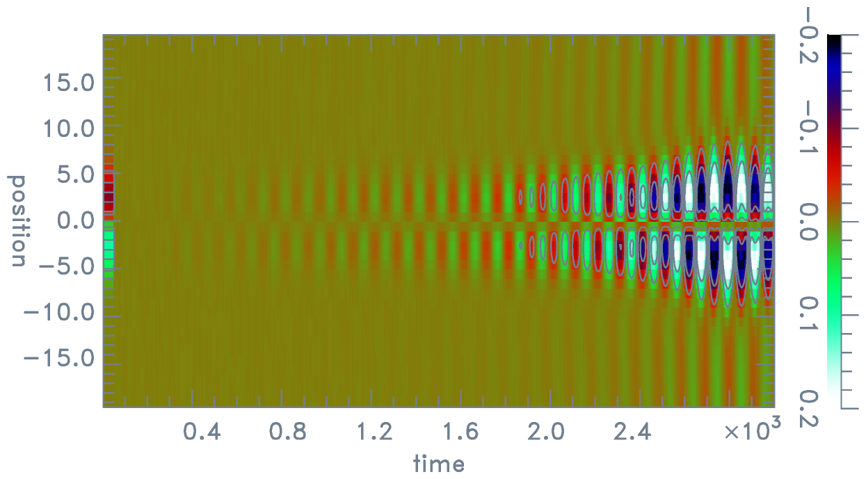
Figure 5: Color (shaded) contours over the indicated range of the oscillating mode ($j=$)8 amplitude $A_{8}(t,z)$ for case $\psi=0.8$, $nz=512$, $ny=238$, showing its growth and spatial variation over the central region $|z|\leq 20$.

In the table the $A_{max}$ column gives the mode’s maximum amplitude (times 100 for compactness); and the ‘time’ column refers to the time the growing mode is largest, which for large amplitudes ($\gtrsim 10$) is before the end of the actual run when nonlinear behavior sets in, but for small or non-growing cases is the run duration (and Mode and $A_{max}$ then refer to the largest amplitude during the run).

The growing mode illustrated in Fig. 5 saturates at time approximately 2600. An arbitrarily scaled template exactly equal to the shift mode replaces the first 20 time slots of the contour plot. The shape of the later actual local perturbation is rather similar to it, but is accompanied by a synchronized wave component consisting of a low-amplitude potential perturbation almost uniform in space beyond $|z|\gtrsim 10$. Prior to saturation there appears to be approximately a 90 degree phase shift between the wave and the shift perturbation, but as saturation occurs the wave becomes closer to 180 degrees out of phase with the shift.

For shallower holes, $\psi<0.4$, no long-term exponentiation was definitively observed, even in cases run for as long as $t=10000$. The very strong scaling of the hole force $\tilde{F}\sim\psi^{13/4}$ and the lower growth rates means lower $\psi$ cases are more affected by noise or other simulation inaccuracies. However, the high computational cost of long duration, low-$\psi$, simulations discouraged more thorough investigation, and it cannot definitively be concluded that there is never instability for $\psi<0.4$.

The oscillatory period (${2\pi\over\omega_{r}}$) and growth time ($1\over\omega_{i}$) of clear instabilities, when present, are documented in the table. Their uncertainty is conservatively estimated at $\pm 10$% and $\pm 20$% respectively. Several of the scaled forms of these parameters are also given. We observe that $\hat{\omega}_{r}$ increases as the hole depth is decreased, to as much as a factor of 2 above what is predicted by the analysis; and $\hat{\omega}_{i}$ to as much as a factor of 4; although the ratio $\hat{\omega}_{i}/\hat{\omega}_{r}^{2}$ remains constant as predicted. The ratio $\hat{k}/\hat{\omega}_{r}$, which according to analysis depends only on the real part of the force, varies little, lying typically only 15% below the value 3.5 the analysis predicts. Thus, we have good confirmation of the real part of the force analysis.

The instability occurring at somewhat higher $\omega$ than predicted by analysis would be expected if the resonant stabilizing force is weaker, because the effective $\partial f_{0}/\partial W|_{R}$ is reduced. Sorting particles in the simulation by total energy ($W=-\phi+v^{2}/2$) shows that the noise level of $\phi$ is sufficient to broaden the apparent energy distribution by an amount of order 0.01 ($T_{e}$ units), presumably flattening the effective $f_{0}$ near its slope discontinuity at $W=0$. The resonant energy is $-W\simeq 2\omega_{r}^{2}=2\hat{\omega}_{r}^{2}\psi^{3/2}$ which is of order 0.004 or less. Therefore the $\phi$ noise is clearly capable of a strong influence on the relevant resonant part of the distribution function, and would be expected to reduce the slope $\partial f_{0}/\partial W|_{R}$. Perhaps it does so by the factor of 4 required to explain the $\omega_{i}$ enhancement, but it does not seem possible to prove this hypothesis definitively. The resonance physics is clearly very hard to reproduce and document in a simulation because of the smallness of the resonant energy, and the slope discontinuity at $W=0$. Alternatively the stabilizing force might be weakened by differences of the eigenmode from the pure shift, for example as a result of the coupled wave component. Detailed consideration of such effects is beyond the present scope.

6 Summary

Theoretical analysis shows that there is a shift-mode kink instability, having low real frequency and very low growth rate, of an initially planar electron hole at high magnetization ($\Omega\gtrsim 5\omega_{p}$ in dimensional units). For a hole of potential form $\phi=\psi\,{\rm sech}^{4}(z/4\lambda_{D})$, the predicted values of the fastest growing mode are $\omega_{r}/\omega_{p}\simeq 0.06(e\psi/T_{e})^{3/4}$, $\omega_{i}/\omega_{p}\simeq 0.001(e\psi/T_{e})^{3/2}$, and $k\lambda_{D}=3.5\omega_{r}/\omega_{p}(e\psi/T_{e})\simeq 0.2(e\psi/T_{e})^{1/4}$.

A simple but accurate new approximation $\omega_{b}/\omega_{p}=\sqrt{-W/2T_{e}}$ for the dependence of bounce frequency $\omega_{b}$ on trapped particle energy $W$ (for small $|W|$) undergirds these purely analytic results. Numerical evaluation of the solution of the Vlasov equation confirms the resulting identification of the three predominant force terms giving rise to the instability as: (1) the intrinsically imaginary part of the jetting of passing particles (which is destabilizing), (2) the imaginary part of the trapped particle resonant term (which is stabilizing), balanced against (3) the imaginary part of the frequency affecting the (otherwise) real total jetting.

Particle in cell simulations show good agreement with the predicted $\omega_{r}$ and $k$, but faster growth by factors of 2 - 4. This discrepancy appears explicable by non-ideal effects in the simulation affecting the trapped distribution function, because the resonant energy is extremely close to zero. Proximity to the distribution slope theoretical discontinuity at the separatrix can be expected to substantially reduce the effective positive slope of the trapped distribution, reducing stabilization. The observed sensitivity of the simulation results to small changes in domain size suggests that hole coupling to the observed long wavelength external waves is significant in them. However, the instability mechanism analyzed does not depend on that coupling. The interpretation proposed is that the hole-wave coupling is a sub-dominant effect of an instability occurring in the hole itself. In that case, the instability can be expected to occur in space plasmas whose domains do not impose the restrictive boundaries and resulting resonant parallel wavelengths of simulations.

The strong reduction in growth rate as the hole depth ($\psi$) is reduced predicts that shallow holes can be very long lived indeed. Moreover if a hole has transverse extent $L_{y}$ insufficient to accommodate the highest unstable wavenumber $k_{max}\simeq 0.3(e\psi/T_{e})^{1/4}/\lambda_{D}$, because $k_{max}L_{y}<2\pi$, then presumably it will be fully stable.

7 Acknowledgements

I am grateful to Xiang Chen for pointing out the closed form solution eq. (20) for the distribution function. This work was partially supported by NASA grant NNX16AG82G. PIC simulations were carried out on the MIT-PSFC partition of the Engaging cluster at the MGHPCC facility (www.mghpcc.org) which was funded by DoE grant number DE-FG02-91-ER54109.

References

- Andersson et al. [2009] Andersson, L., Ergun, R. E., Tao, J., Roux, A., Lecontel, O., Angelopoulos, V., Bonnell, J., McFadden, J. P., Larson, D. E., Eriksson, S., Johansson, T., Cully, C. M., Newman, D. N., Goldman, M. V., Glassmeier, K. H. & Baumjohann, W. 2009 New features of electron phase space holes observed by the THEMIS mission. Physical Review Letters 102 (22), 225004.
- Bale et al. [1998] Bale, S. D., Kellogg, P. J., Larsen, D. E., Lin, R. P., Goetz, K. & Lepping, R. P. 1998 Bipolar electrostatic structures in the shock transition region: Evidence of electron phase space holes. Geophysical Research Letters 25 (15), 2929–2932.
- Berk et al. [1970] Berk, H. L., Nielsen, C. E. & Roberts, K. V. 1970 Phase Space Hydrodynamics of Equivalent Nonlinear Systems: Experimental and Computational Observations. Physics of Fluids 13 (4), 980.
- Bernstein et al. [1957] Bernstein, I. B., Greene, J. M. & Kruskal, M. D. 1957 Exact nonlinear plasma oscillations. Physical Review 108 (4), 546–550.
- Berthomier et al. [2002] Berthomier, M., Muschietti, L., Bonnell, J. W., Roth, I. & Carlson, C. W. 2002 Interaction between electrostatic whistlers and electron holes in the auroral region. Journal of Geophysical Research: Space Physics 107 (A12), 1–11.
- Eliasson & Shukla [2006] Eliasson, B. & Shukla, P. K. 2006 Formation and dynamics of coherent structures involving phase-space vortices in plasmas. Physics Reports 422 (6), 225–290.
- Ergun et al. [1998] Ergun, R. E., Carlson, C. W., McFadden, J. P., Mozer, F. S., Muschietti, L., Roth, I. & Strangeway, R. J. 1998 Debye-Scale Plasma Structures Associated with Magnetic-Field-Aligned Electric Fields. Physical Review Letters 81 (4), 826–829.
- Goldman et al. [1999] Goldman, M. V., Oppenheim, M. M. & Newman, D. L. 1999 Nonlinear two-stream instabilities as an explanation for auroral bipolar wave structures. Geophysical Research Letters 26 (13), 1821–1824.
- Hutchinson [2011] Hutchinson, I. H. 2011 Nonlinear collisionless plasma wakes of small particles. Phys. Plasmas 18, 032111.
- Hutchinson [2017] Hutchinson, I. H. 2017 Electron holes in phase space: What they are and why they matter. Physics of Plasmas 24 (5), 055601.
- Hutchinson [2018a] Hutchinson, I. H. 2018a Kinematic Mechanism of Plasma Electron Hole Transverse Instability. Physical Review Letters 120 (20), 205101.
- Hutchinson [2018b] Hutchinson, I. H. 2018b Transverse instability of electron phase-space holes in multi-dimensional Maxwellian plasmas. Journal of Plasma Physics 84, 905840411, arXiv: 1804.08594.
- Hutchinson [2019] Hutchinson, I. H. 2019 Transverse instability magnetic field thresholds of electron phase-space holes. Physical Review E 99, 053209.
- Hutchinson et al. [2015] Hutchinson, I. H., Haakonsen, C. B. & Zhou, C. 2015 Non-linear plasma wake growth of electron holes. Physics of Plasmas 22 (3), 32312.
- Hutchinson & Malaspina [2018] Hutchinson, I. H. & Malaspina, D. M. 2018 Prediction and Observation of Electron Instabilities and Phase Space Holes Concentrated in the Lunar Plasma Wake. Geophysical Research Letters 45, 3838–3845.
- Hutchinson & Zhou [2016] Hutchinson, I. H. & Zhou, C. 2016 Plasma electron hole kinematics. I. Momentum conservation. Physics of Plasmas 23 (8), 82101.
- Jovanović & Schamel [2002] Jovanović, D. & Schamel, H. 2002 The stability of propagating slab electron holes in a magnetized plasma. Physics of Plasmas 9 (12), 5079–5087.
- Lu et al. [2008] Lu, Q. M., Lembege, B., Tao, J. B. & Wang, S. 2008 Perpendicular electric field in two-dimensional electron phase-holes: A parameter study. Journal of Geophysical Research 113 (A11), A11219.
- Malaspina et al. [2014] Malaspina, D. M., Andersson, L., Ergun, R. E., Wygant, J. R., Bonnell, J. W., Kletzing, C., Reeves, G. D., Skoug, R. M. & Larsen, B. A. 2014 Nonlinear electric field structures in the inner magnetosphere. Geophysical Research Letters 41, 5693–5701.
- Malaspina et al. [2013] Malaspina, D. M., Newman, D. L., Willson, L. B., Goetz, K., Kellogg, P. J. & Kerstin, K. 2013 Electrostatic solitary waves in the solar wind: Evidence for instability at solar wind current sheets. Journal of Geophysical Research: Space Physics 118 (2), 591–599.
- Mangeney et al. [1999] Mangeney, A., Salem, C., Lacombe, C., Bougeret, J.-L., Perche, C., Manning, R., Kellogg, P. J., Goetz, K., Monson, S. J. & Bosqued, J.-M. 1999 WIND observations of coherent electrostatic waves in the solar wind. Annales Geophysicae 17 (3), 307–320.
- Matsumoto et al. [1994] Matsumoto, H., Kojima, H., Miyatake, T., Omura, Y., Okada, M., Nagano, I. & Tsutsui, M. 1994 Electrostatic solitary waves (ESW) in the magnetotail: BEN wave forms observed by GEOTAIL. Geophysical Research Letters 21 (25), 2915–2918.
- Miyake et al. [1998] Miyake, T., Omura, Y., Matsumoto, H. & Kojima, H. 1998 Two-dimensional computer simulations of electrostatic solitary waves observed by Geotail spacecraft. Journal of Geophysical Research 103 (A6), 11841.
- Morse & Nielson [1969] Morse, R. L. & Nielson, C. W. 1969 One-, two-, and three-dimensional numerical simulation of two-Beam plasmas. Physical Review Letters 23 (19), 1087–1090.
- Mottez et al. [1997] Mottez, F., Perraut, S., Roux, A. & Louarn, P. 1997 Coherent structures in the magnetotail triggered by counterstreaming electron beams. Journal of Geophysical Research 102 (A6), 11399.
- Mozer et al. [2016] Mozer, F. S., Agapitov, O. A., Artemyev, A., Burch, J. L., Ergun, R. E., Giles, B. L., Mourenas, D., Torbert, R. B., Phan, T. D. & Vasko, I. 2016 Magnetospheric Multiscale Satellite Observations of Parallel Electron Acceleration in Magnetic Field Reconnection by Fermi Reflection from Time Domain Structures. Physical Review Letters 116 (14), 4–8, arXiv: arXiv:1011.1669v3.
- Mozer et al. [2018] Mozer, F. S., Agapitov, O. V., Giles, B. & Vasko, I. 2018 Direct Observation of Electron Distributions inside Millisecond Duration Electron Holes. Physical Review Letters 121 (13), 135102.
- Muschietti et al. [2000] Muschietti, L., Roth, I., Carlson, C. W. & Ergun, R. E. 2000 Transverse instability of magnetized electron holes. Physical Review Letters 85 (1), 94–97.
- Newman et al. [2001] Newman, D. L., Goldman, M. V., Spector, M. & Perez, F. 2001 Dynamics and instability of electron phase-space tubes. Physical Review Letters 86 (7), 1239–1242.
- Oppenheim et al. [1999] Oppenheim, M., Newman, D. L. & Goldman, M. V. 1999 Evolution of Electron Phase-Space Holes in a 2D Magnetized Plasma. Physical Review Letters 83 (12), 2344–2347.
- Oppenheim et al. [2001] Oppenheim, M. M., Vetoulis, G., Newman, D. L. & Goldman, M. V. 2001 Evolution of electron phase-space holes in 3D. Geophysical Research Letters 28 (9), 1891–1894.
- Pickett et al. [2008] Pickett, J. S., Chen, L.-J., Mutel, R. L., Christopher, I. W., Santolı´k, O., Lakhina, G. S., Singh, S. V., Reddy, R. V., Gurnett, D. A., Tsurutani, B. T., Lucek, E. & Lavraud, B. 2008 Furthering our understanding of electrostatic solitary waves through Cluster multispacecraft observations and theory. Advances in Space Research 41 (10), 1666–1676.
- Schamel [1986] Schamel, H. 1986 Electrostatic Phase Space Structures in Theory and Experiment. Physics Reports 140 (3), 161–191.
- Singh et al. [2001a] Singh, N., Loo, S. M. & Wells, B. E. 2001a Electron Hole as an Antenna Radiating PlasmaWaves. Geophysical Research Letters 28 (7), 1371–1374.
- Singh et al. [2001b] Singh, N., Loo, S. M. & Wells, B. E. 2001b Electron hole structure and its stability depending on plasma magnetization. Journal of Geophysical Research 106 (A10), 21183–21198.
- Turikov [1984] Turikov, V. A. 1984 Electron Phase Space Holes as Localized BGK Solutions. Physica Scripta 30 (1), 73–77.
- Umeda [2008] Umeda, T. 2008 Generation of low-frequency electrostatic and electromagnetic waves as nonlinear consequences of beam – plasma interactions. Physics of Plasmas 15, 064502.
- Umeda et al. [2006] Umeda, T., Omura, Y., Miyake, T., Matsumoto, H. & Ashour-Abdalla, M. 2006 Nonlinear evolution of the electron two-stream instability: Two-dimensional particle simulations. Journal of Geophysical Research: Space Physics 111 (10), 1–9.
- Vasko et al. [2015] Vasko, I. Y., Agapitov, O. V., Mozer, F., Artemyev, A. V. & Jovanovic, D. 2015 Magnetic field depression within electron holes. Geophysical Research Letters 42 (7), 2123–2129.
- Vetoulis & Oppenheim [2001] Vetoulis, G. & Oppenheim, M. 2001 Electrostatic mode excitation in electron holes due to wave bounce resonances. Physical Review Letters 86 (7), 1235–1238.
- Wilson et al. [2010] Wilson, L. B., Cattell, C. A., Kellogg, P. J., Goetz, K., Kersten, K., Kasper, J. C., Szabo, A. & Wilber, M. 2010 Large-amplitude electrostatic waves observed at a supercritical interplanetary shock. Journal of Geophysical Research: Space Physics 115 (12), A12104.
- Wu et al. [2010] Wu, M., Lu, Q., Huang, C. & Wang, S. 2010 Transverse instability and perpendicular electric field in two-dimensional electron phase-space holes. Journal of Geophysical Research: Space Physics 115 (10), A10245.
- Zhou & Hutchinson [2017] Zhou, C. & Hutchinson, I. H. 2017 Plasma electron hole ion-acoustic instability. J. Plasma Phys. 83, 90580501, arXiv: arXiv:1701.03140v1.