On the Insufficiency of the Large Margins Theory in Explaining the Performance of Ensemble Methods

Abstract

Boosting and other ensemble methods combine a large number of weak classifiers through weighted voting to produce stronger predictive models. To explain the successful performance of boosting algorithms, Schapire et al. (1998) showed that AdaBoost is especially effective at increasing the margins of the training data. Schapire et al. (1998) also developed an upper bound on the generalization error of any ensemble based on the margins of the training data, from which it was concluded that larger margins should lead to lower generalization error, everything else being equal (sometimes referred to as the “large margins theory”). Tighter bounds have been derived and have reinforced the large margins theory hypothesis. For instance, Wang et al. (2011) suggest that specific margin instances, such as the equilibrium margin, can better summarize the margins distribution. These results have led many researchers to consider direct optimization of the margins to improve ensemble generalization error with mixed results. We show that the large margins theory is not sufficient for explaining the performance of voting classifiers. We do this by illustrating how it is possible to improve upon the margin distribution of an ensemble solution, while keeping the complexity fixed, yet not improve the test set performance.

1 Introduction

Ensemble methods, such as boosting  (Schapire, 1990), bagging (Breiman, 1996a) and random forests  (Breiman, 2001), along with their variants [see, e.g., stochastic gradient boosting  (Friedman, 2002), rotation forests  (Rodriguez et al., 2006), extreme gradient boosting  (Chen and Guestrin, 2016)] create a set of weak classifiers, which are typically decision trees, then combine the predictions from these classifiers in the form of a weighted vote to produce an improved prediction. Empirical evidence suggests that these ensemble methods have lower generalization error than the individual classifiers (Drucker et al., 1994; Dietterich, 2000; Breiman, 2001; Maclin and Opitz, 2011). Recently, ensembles have gained further popularity by winning most of the top machine learning competitions in competition platforms such as Kaggle  (Hong et al., 2014; Puurula et al., 2014; Graham, 2015; Hoch, 2015; Wang et al., 2015; Nielsen, 2016; Zou et al., 2017) and being applied into a wide range of problems (See e.g.,  Richardson 2000; Coussement and De Bock 2013; King et al. 2014; Weng et al. 2018b, a). Much theoretical work has been done to explain why ensemble methods are so successful and also why the seemingly complex models often do not overfit (Breiman, 1996b; Schapire et al., 1998; Buja, 2000; Breiman, 2000; Mease and Wyner, 2008). In particular, upper bounds on the generalization error of ensemble classifiers based on margins have been developed, which point to margins as a key determinant of ensemble performance. It has been suggested by Schapire et al. (1998) and Reyzin and Schapire (2006), among others, that larger margins should result in better ensemble performance, everything else being equal. This has led many researchers to consider directly optimizing the margins to improve ensemble generalization error (see, e.g.,  Grove and Schuurmans 1998; Breiman 1999; Mason et al. 2000; Rätsch and Warmuth 2002; Shen and Li 2010; Zhou 2014). Direct optimization of margins has not necessarily yielded successful results, but research is ongoing  (Schapire, 2013). Other researchers  (Wang et al., 2011, 2012; Gao and Zhou, 2013) have provided different generalization error bounds based on functions or particular measures of the margins instances in an attempt to make the theory more complete. In this paper we develop a method for reweighting the weak classifiers of an ensemble in such a way as to increase or maintain all of the margins of a given ensemble solution. According to the large margins theory, this should result in improved performance (lower generalization error) for the combined classifier, if other factors, such as the complexity of the base learners, are held constant. We discover though, that the gains in improved performance are not realized, even when all of the margins of a particular ensemble solution are improved. This leads us to the conclusion that the large margins theory, as currently stated, is insufficient for explaining boosting and ensemble performance. In the next section, we discuss margins, the generalization error bounds based on margins, and the large margins theory. In section 3, we show how to use linear programming techniques to improve or maintain all of the margins of an ensemble and provide empirical evidence to show that this does not necessarily lead to improved ensemble performance. A simulation study is performed and analyzed in section 4. Finally, we discuss our results and their implications for the large margins theory in section 5.

2 Preliminaries

We assume we are given a training sample of data pairs $S=\{(\textbf{x}_{1},y_{1}),…,(\textbf{x}_{n},y_{n})\}$ generated independently and identically distributed (i.i.d) according to an unknown distribution $P_{XY}$ with joint density $p(\textbf{x},y)$, where $Y\in\left\{-1,+1\right\}$ is a binary response variable and $\textbf{x}\in\mathbb{R}^{p}$. The general goal of learning is to estimate a function $H:X\rightarrow Y$ such that $H$ will correctly classify unseen examples $(\textbf{x},y)$. The function is selected such that the generalization error $R[H]$ (also called the expected risk of the function) is minimized:

$$R[H]=E_{\textbf{x},y}g(y,H(\textbf{x}))=\int g(y,H\left(\textbf{x}\right))dp(\textbf{x},y),$$ (1)

where $g(y,H(\textbf{x}))$ is a suitable loss function. For binary classification the loss function $I(y_{i}\neq H(\textbf{x}))$ is typically used, where $I(y_{i}\neq H(\textbf{x}))=1$ if $(y_{i}\neq H(\textbf{x}))$, 0 otherwise. The generalization error cannot be minimized directly because the underlying distribution $P_{XY}$ is unknown. The minimum theoretical value of $R[H]$ is often referred to as Bayes’ minimum risk. $R[H]$ is approximated by the empirical error of the training data set $\hat{R}[H]=\frac{1}{n}\sum g(y,H\left(\textbf{x}\right))$.

We refer to $P[.]$ as probabilities with respect to $P_{XY}$ and $\hat{P}[.]$ as the probability with respect to the empirical distribution over the sample $S$. We assume a set of $T$ classifiers $h_{t}(\textbf{x}),t=1,2,...,T$, is created from the space of classifiers $\mathscr{H}$, where $\mathscr{\left|H\right|}<\infty$. The classifiers are usually called base learners, weak learners or weak classifiers, and they are generated from the training data by a base-learning algorithm B. Each classifier takes a $p\times 1$ input vector x and produces a prediction $h_{t}(\textbf{x})\in\{-1,+1\}$ for a binary response variable $Y$. The combined classifier of the prediction is given by the linear function:

$$H(\textbf{x})=sign\left(\sum_{t=1}^{T}\alpha_{t}h_{t}(\textbf{x})\right)$$ (2)

where $sign:\mathbb{R}\rightarrow\left(-1,+1\right)$, such that $sign(x)=-1$ when $x<0$, $+1$ otherwise, $\alpha_{t}$ is the weight associated with the $t^{th}$ weak classifier. Without loss of generality, we can assume $0\leq\alpha_{t}\leq 1$ and $\sum_{t=1}^{T}\alpha_{t}=1$.

The AdaBoost algorithm (ADA) is arguably the best-known boosting algorithm and one of the most used ensemble methods. Unlike earlier boosting methods (Schapire 1990; Freund 1995), AdaBoost adjusts adaptively to the errors of the weak classifiers (hence the name Adaptive Boosting). AdaBoost is described in Algorithm 1. The task of a boosting is to create a set of weak classifiers and determine their associated weights ${\alpha_{1},...,\alpha_{T}}$ based on the training sample of data $S$, to produce a combined prediction with small generalization error $R[H]$. Many researchers have pointed out the margins of the observations as important characteristics of why the AdaBoost algorithm and most ensemble methods outperform individual classifiers. The $i^{th}$ margins of an observation is given by:

$$m_{i}=y_{i}\sum_{t=1}^{T}\alpha_{t}h_{it}(\textbf{x}_{i}).$$ (3)

A large positive margin of the $i^{th}$ training observation can be viewed as a measure of “confidence” in the prediction for the $i^{th}$ training observation (Schapire et al., 1998). The margin of the $i^{th}$ observation is equal to the difference in the weighted proportion of weak classifiers correctly predicting the $i^{th}$ observation and the weighted proportion of weak classifiers incorrectly predicting the $i^{th}$ observation, so that $-1\leq m_{i}\leq 1$. A margin value of $-1$ indicates that all of the weak classifiers’ predictions were incorrect, while a margin value of $+1$ indicates all of the weak classifiers correctly predicted the observation.

Algorithm 1 AdaBoost (ADA)

1:procedure ADA($S,T$)

2:     $D_{i}^{(1)}\leftarrow\frac{1}{n}$

3:     do for $t=1,...,T$

4:     (a) $h_{t}(\textbf{x}_{i}))\leftarrow h(\{S,D^{(t)}\})$

5:     (b) $\epsilon_{t}\leftarrow\sum_{i=1}^{n}D_{i}^{(t)}I\left(y_{i}\neq h_{t}(\textbf{x}_{i})\right)$

6:     (c) break if $\epsilon_{t}=0$ or $\epsilon_{t}\geq\frac{1}{2}$

7:     (d) $\alpha_{t}\leftarrow\frac{1}{2}\ln\left(\frac{1-\epsilon_{t}}{\epsilon_{t}}\right)$

8:     (e) $D_{i}^{(t+1)}\leftarrow\frac{D_{i}^{(t)}\exp\{-\alpha_{t}y_{i}h_{t}(\textbf{x}_{i})\}}{Z_{t}}$

9:     end for

10:     $H{\textbf{(x)}}=sign\left(\sum_{t=1}^{T}\alpha_{t}h_{t}(\textbf{x})\right)$

11:return $H{\textbf{(x)}}$

The development of boosting algorithms was based on the PAC learning theory (Valiant, 1984). It has been shown that AdaBoost is a PAC (strong) learner. as defined below:

Definition 1 (Valiant, 1984). Let $\mathscr{F}$ be a class of concepts. For every distribution $P_{XY}$, all concepts $f\in\mathscr{F}$ and all $\epsilon\in(0,1/2)$, $\delta\in(0,1/2)$, a strong PAC learner has the property that with probability at least $1-\delta$ the base learning algorithm B outputs a hypothesis $h$ with $P\left(h(\textbf{x})\neq f(\textbf{x})\right)\leq\epsilon$. B must run in polynomial time in $1/\epsilon$, and $1/\delta$ using only a polynomial (in $1/\epsilon$ and $1/\delta$) number of examples.

A weak learner drops the strong accuracy requirement, that is, to output a hypothesis $h$ with $P\left(h(\textbf{x})\neq f(\textbf{x})\right)\leq\epsilon$ with a probability of at least $1-\delta$, and replaces it with the requirement that the algorithm outputs a hypothesis that performs better than random guessing.

3 Generalization Error Bounds Based on Margins

Boosting is based on the question posed by Kearns and Valiant (1994) about whether weak and strong learning are equivalent for efficient learning algorithms. In the development of the first algorithm that adaptively boosted a weak learner into a stronger performing algorithm, Freund and Schapire (1997) answered this question and also gave a bound on the generalization error of boosting in terms of the number of boosting rounds $T$, the VC-dimension $d$ (a measure of complexity) and the training set error rate $\hat{P}\left[H(\textbf{x})\neq y\right]$. (See Freund and Schapire 1997 for the derivation of the bound.) They showed the generalization error, with high probability, was bounded by

$$R[H]\leq\hat{P}\left[H(\textbf{x})\neq y\right]+O\left(\sqrt{\frac{Td}{n}}\right).$$ (4)

The bound in (4) suggests the generalization error would degrade as the number of rounds of boosting $T$ increased. This in fact happens, especially in cases where there is noise, (see, e.g., Grove and Schuurmans 1998; Dietterich 2000; Long and Servedio 2010; Martinez and Gray 2016), but under certain conditions boosting methods have shown not to overfit even when thousands of rounds are run (see, e.g., Breiman 1996b; Drucker and Cortes 1996; Quinlan 1996; Grove and Schuurmans 1998; Opitz and Maclin 1999; Buja 2000; Lugosi and Vayatis 2004). To better explain the effectiveness of AdaBoost and other ensembles, Schapire et al. (1998) developed an upper bound on the generalization error of any ensemble method, based on the margins of the training data, from which it was concluded that larger margins should lead to a lower generalization error of the ensemble, everything else being equal. This bound does not depend on the number of rounds $T$ and is summarized in theorem 1.

Bound 1(Schapire et al., 1998). Assuming that the base-classifier space $\mathscr{H}$ is finite, and for any $\delta>0$ and $\theta>0$, then with probability at least $1-\delta$ over the training set $S$ with size $n$, every voting classifier $H$ satisfies the following bound:

$$R[H]\leq\hat{P}\left[m(\textbf{x},y)\leq\theta)\right]+O\left(\frac{1}{\sqrt{n}}\sqrt{\frac{\ln{n}\ln{\mathscr{\left|H\right|}}}{\theta^{2}}+\ln{\frac{1}{\delta}}}{}\right),$$ (5)

where the term $\hat{P}\left[m(\textbf{x},y)\leq\theta)\right]$ is the proportion of training margins less than an arbitrary value $\theta>0$, and $\mathscr{\left|H\right|}$ refers to the cardinality of the finite hypothesis space. When the hypothesis space is infinite, the term $\ln{n}\ln{\mathscr{\left|H\right|}}$ is replaced by $d\log_{2}(d/n)$, where $d$ is the VC-dimension of the space of all possible weak classifiers. Schapire et al. (1998) use this bound to provide an explanation for the superior performance of AdaBoost, which they show is highly effective at increasing the margins.

Even though the upper bound in (5) is quite loose in most practical situations (Breiman, 1999), researchers have used it to conclude that higher margins should lead to a lower generalization error rate, everything else being equal. For example, Reyzin and Schapire (2006) state that “the margins explanation basically says that when all other factors are equal, higher margins result in lower error.” This interpretation of the upper bound in (5) has been referred to as the “large margins theory" in the boosting literature. (see, e.g., Schapire et al. 1998; Grove and Schuurmans 1998; Mason et al. 2000; Wang et al. 2011; Shen and Li 2010; Wang et al. 2011; Cid 2012; Wang et al. 2012; Gao and Zhou 2013; Martinez and Gray 2014; Liu and Liao 2015; Martinez and Gray 2019; and Zhang and Zhou 2016 for further insight into the importance of large margins in ensemble performance.) Unfortunately, much of the boosting literature is replete with phrases like “higher margins”, “large margins for most of the examples”, “maximizing the number of training examples with large margins”, and “maximizing the margins” without specific, operational definitions of these terms (see, e.g., Schapire et al. 1998). Grove and Schuurmans (1998) and others, initially defined “maximizing the margin” as maximizing the minimum margin. Their linear programming approach, LP-Boost, is designed to maximize the minimum margin by optimizing the weights associated with the weak learners. Breiman (1999), for instance, developed a new boosting algorithm, called arc-gv, which he proved maximizes the minimum margin. Instead of using direct optimization of the margin, Breiman (1999) modified the weights of the individual classifiers to be updated to

$$\alpha^{*}_{t}=\frac{1}{2}\ln\left(\frac{1+\gamma_{t}}{1-\gamma_{t}}\right)-\frac{1}{2}\ln\left(\frac{1+\rho_{t}}{1-\rho_{t}}\right),$$ (6)

where $\gamma_{t}=\sum_{i=1}^{n}D_{i}^{t}y_{i}h_{t}(\textbf{x}_{i})$ is called the edge of $h_{t}$, and $\rho_{t}=\min\left(y_{i}\sum_{t=1}^{T}\alpha^{*}_{t}h_{t}(\textbf{x}_{i})\right)$. Note that in Algorithm 1, the unnormalized $\alpha_{t}$ weights can be expressed as $\alpha_{t}=\frac{1}{2}\ln\left(\frac{1+\gamma_{t}}{1-\gamma_{t}}\right)$, so that (6) updates the original $\alpha_{t}$ with information on the minimum margin over all training examples. Breiman also presented a bound on the generalization error of any voting classifier based on the minimum margin that was tighter than that presented by Schapire et al. (1998). Breiman (1999) found in his experiments that arc-gv not only produced larger minimum margins over all training examples, but it also produced a better margin distribution than AdaBoost (see Figure 1), however, he discovered that the test set error performance of arc-gv was typically worse than for AdaBoost. Breiman (1999) noted that the upper bounds on the generalization error of ensembles proposed by Schapire et al. (1998) and Breiman (1999) are “greater than one in all practical cases, leaving ample room for other factors to influence the true generalization error” and concluded that this “casts doubt on the ability of the loose VC-type bounds to uncover the mechanism leading to low generalization error.” Breiman (1999) concluded that the large margins theory was incorrect based on his findings.

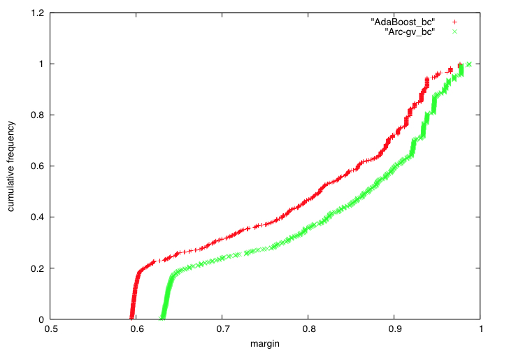
Figure 1: Reprinted from Reyzin and Schapire (2006) with permission (permission will be obtained prior to publication). Cumulative margins for AdaBoost and arc-gv for the breast cancer data set after 500 iterations.

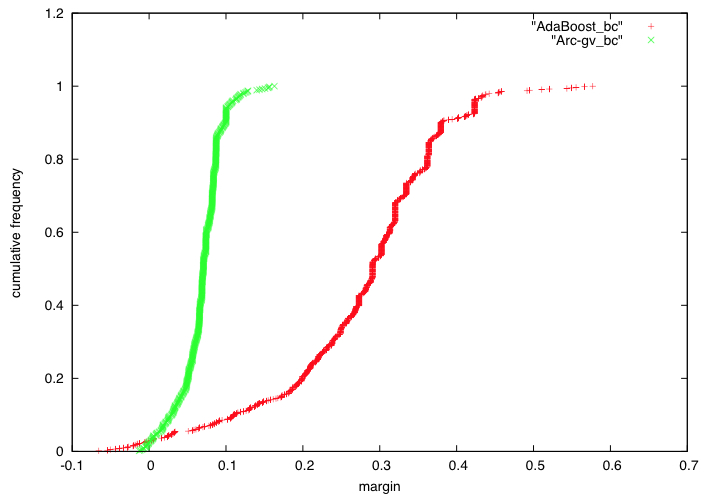
Figure 2: Reprinted from Reyzin and Schapire (2006) with permission (permission will be obtained prior to publication). Cumulative margins for AdaBoost and arc-gv for the breast cancer data set after 100 iterations using decision stumps.

Reyzin and Schapire (2006) replicated the analysis presented in Breiman (1999), but pointed out that the trees (weak classifiers) found by arc-gv were deeper on average than the trees generated by AdaBoost, even though the number of terminal nodes was kept the same. They concluded that this increased complexity could have led to overfitting by arc-gv, and hence the worse test set performance. More importantly, Reyzin and Schapire (2006) suggested that the increased complexity in the trees generated by arc-gv violated the assumption of everything else kept constant, discrediting Breiman’s evidence against the large margins theory. When Reyzin and Schapire (2006) limited both arc-gv and AdaBoost to decision stumps, it was found that while arc-gv did have a larger minimum margin than AdaBoost, it did not produce uniformly higher margins (see Figure 2), furthering their conclusion that the large margins theory was still intact. Reyzin and Schapire (2006) also concluded that maximizing the minimum margin does not necessarily result in improved generalization error.

After the less-than-satisfactory results from maximizing the minimum margin, many authors have supported the large margins theory and have proposed optimizing other functions of the margin distribution. Reyzin and Schapire (2006) suggested maximizing the average or the median margin. Mason et al. (2000) proposed the DOOM (Direct Optimization of Margins) algorithm, which optimizes the average of a cost function of the margins. DOOM outperformed AdaBoost in most of the examples considered. They also showed that the size of the minimum margin was not a critical factor in generalization error. Shen and Li (2010) suggested an algorithm named MD-Boost (Margin Distribution Boosting), which attempts to maximize the average margin while minimizing the variance of the margin distribution. Shen and Li (2010) provide evidence that MD-Boost outperforms AdaBoost in many of the UCI Repository data sets, however it is worth mentioning that the margins produced by MD-Boost are not uniformly larger than those of AdaBoost and consequently the MD-Boost margin distributions are not uniformly larger than those of AdaBoost. Other researchers have summarized the margin distribution of an ensemble on a single metric. For example, Wang et al. (2011) provided an upper bound for the generalization error of ensemble methods based on a new margin notion referred to as the equilibrium margin (EMargin). To better understand the bound, we introduce the Bernoulli Kullback-Leibler function $D(q\left|\right|p)$ defined as

$$D(q\left|\right|p)\leq q\ln\frac{q}{p}+(1-q)\ln\frac{1-q}{1-p},0\leq p,q\leq 1.$$ (7)

$D(q\left|\right|p)$ is a monotone increasing function for a fixed $q$ and $q\leq p<1$. We can also see that $D(q\left|\right|p)=0$ when $p=q$ and $D(q\left|\right|p)\rightarrow\infty$ as $p\rightarrow 1$. The bound is presented in Theorem 3.

Theorem 3 (Wang et al., 2011). Assuming that the base-classifier space $\mathscr{\left|H\right|}$ is finite, and for any $\delta>0$ and $\theta>0$, then with probability at least $1-\delta$ over the training set $S$ with size $n$, every voting classifier $H$ satisfies the following bound:

$$R[H]\leq\frac{\ln{\mathscr{\left|H\right|}}}{n}+\inf_{q\in\left(0,\frac{1}{n},\frac{2}{n},...,1\right)}D^{-1}\left(q;u\left[\hat{\theta}(q)\right]\right),$$ (8)

where

$$u\left[\hat{\theta}(q)\right]=\frac{1}{n}\left(\frac{8\ln\mathscr{\left|H\right|}}{\hat{\theta}^{2}(q)}\ln\left(\frac{2n^{2}}{\ln\mathscr{\left|H\right|}}\right)+\ln{\mathscr{\left|H\right|}}+\ln\frac{1}{\delta}\right)$$ (9)

and

$$\hat{\theta}(q)=\sup_{\theta\in\left(\sqrt{\frac{8}{\mathscr{\left|H\right|}}},1\right]}\hat{P}\left[m(\textbf{x},y)\leq\theta)\right]\leq q.$$ (10)

The optimal value of $q$ in (8) defined as $q^{*}$ evaluated at $\hat{\theta}(q^{*})$ is called the equilibrium margin (EMargin), while $q^{*}$ is called the EMargin error. The upper bound developed by Wang et al. (2011) is an explanation of the performance of ensemble methods based on a single characteristic called the EMargin, instead of the margin mean and variance. Wang et al. (2011, 2012) provide evidence that ensembles with higher EMargins, $\hat{\theta}(q^{*})$, or lower in EMargin errors $q^{*}$ would result in a better generalization performance, everything else being equal. In particular they show that AdaBoost’s EMargins are higher in most cases than arc-gv’s (Breiman, 1999), which explains why despite arc-gv’s larger minimum margin, it has worse performance. Wang et al. (2011) give further validation to the conjecture that the whole margin distribution is more important than the minimum margin, and that the margin distribution can be better summarized in the single Emargin characteristic as opposed to the sample moments. Tighter bounds under the large margins theory are commonplace in the recent research literature and beyond the scope of this research. Among the most notable contributions is the bound provided by Gao and Zhou (2013), which suggests that both the bounds in Theorem 2 and Theorem 3 are special cases of the $k^{th}$margin bound. Gao and Zhou (2013) found that the $k^{th}$ margin bound was tighter than the bounds analyzed in Theorem 2 and Theorem 3. Gao and Zhou (2013) further support the idea that the whole margin distribution is the main driver to ensemble method performance and also give further validation to the Emargin notion.

In the next section, we show how it is possible to improve over the margins of an ensemble solution or its EMargin using the same set of weak learners generated by the original ensemble and still not achieve a better generalization performance. It is important to note that this paper does not attempt to prove the large margins theory wrong, but to shed light on the fact that there may be other unknown factors involved in the explanation of ensemble performance.

4 Improving the Margins of an Ensemble

We describe here a method, based on linear programming, for improving or at least maintaining all the margins of any ensemble. We do this by simply updating the weights given to the weak classifiers. Once the entire margin distribution is improved, or at least maintained, any summary location measure of the margins distribution (including the minimum, median, mean, and percentiles) will also be improved or maintained. Thus, the proposed method achieves “higher margins” regardless of the definition. Furthermore, we fix the ensemble complexity by using the same set of trees provided by the ensemble, and also by forcing the trees to grow to a fixed depth and number of terminal nodes $k$. We should mention that our simulations results hold regardless of the selected value of $k$, and that the choices of $k$ here are only meant to provide the reader with a better intuition on how the results hold. The choice of a fixed $k$ for a given depth ensures the complexity is unchanged, and allows us to compute the cardinality of the hypothesis space $\mathscr{\left|H\right|}$ when comparing across methods (Reyzin and Schapire, 2006), but we also provide evidence on how our results hold for unpruned fully-grown trees. Furthermore, by using linear programming, the proposed methods provide an improvement on the overall computational burden of the resulting ensemble solution, as many of the weights are zeroed out by the optimization.

4.1 Maximizing the Minimum Margin Improvement

We assume that we are given an ensemble solution, i.e., a set of weak classifiers $h_{t}(\textbf{x}),t=1,2,...,T$, and a set of weights $\alpha_{t},t=1,2,...,T$, where $0\leq\alpha_{t}\leq 1$ and $\sum_{t=1}^{T}\alpha_{t}=1$, associated with the weak classifiers. Note that for the training sample $\{(\textbf{x}_{i},y_{i}),i=1,2,...,n\}$ used to produce the ensemble solution, the values of the weak classifier predictions and the weights are fixed. We will let $h_{t}(\textbf{x}_{i})=\pm 1$ denote the prediction of the $t^{th}$ weak classifier for the $i^{th}$ observation in the training data when given the covariate vector $\textbf{x}_{i}$. Our goal in the first improvement algorithm, MMI, is optimize the weights associated with the weak classifiers such that we maximize the minimum improvement to the ensemble margins. The linear program (LP) used to achieve this solution is given in Algorithm 2.

Algorithm 2 MMI

$$\begin{array}[]{rl}\max&\xi\\ \mbox{s.t.}&y_{i}\sum{{}_{t=1}^{T}\alpha_{t}^{\prime}h_{t}(\textbf{x}_{i})\geq m_{i}+\xi},i=1,2,...,n\\ &\sum{{}_{t=1}^{T}\alpha_{t}^{\prime}=1}\\ &\alpha_{t}^{\prime}\geq 0,t=1,2,...,T\\ &\xi\geq 0,\end{array}$$

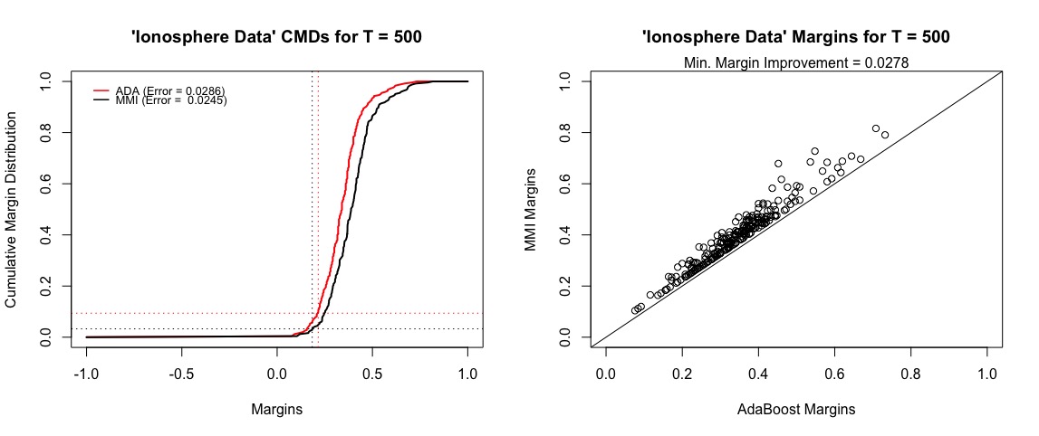
Figure 3: Comparison of AdaBoost and the MMI algorithm for the Ionosphere Data using 750 4-node (depth = 2) trees. The left panel compares the cumulative margin distributions (CMD) for AdaBoost and the MMI algorithm. The dotted lines indicate the Emargins (x-axis) and the Emargin Errors (y-axis). The right panel is a scatter plot of the AdaBoost margins and MMI margins. The line in the graph indicates equality of the margins.

In Algorithm 2 $m_{i}=y_{i}\sum_{t=1}^{T}\alpha_{t}h_{t}(\textbf{x}_{i})$ is the original ensemble margin for the $i^{th}$ observation and $\alpha_{t}^{\prime},t=1,2,...,T$, are the new weights for the weak learners, to be determined by solving the LP. The linear optimization constraint $y_{i}\sum{{}_{t=1}^{T}\alpha_{t}^{\prime}h_{it}(\textbf{x}_{i})\geq m_{i}+\xi}$ for $\xi\geq 0$ guarantees that the choice of $\alpha_{t}^{\prime}$ will produce new margins at least as large as the margins generated by ensemble. To illustrate the performance of the MMI algorithm and compare it to original ensemble solution, we fit an AdaBoost model using 750 weak classifiers (depth = 2, 4-node trees) to the Ionosphere data set, then obtain the updated weights and margins from Algorithm 2. The cumulative margin distributions (CMD) of AdaBoost and MMI are plotted in the left panel of Figure 3. Since the margins generated by the MMI algorithm are uniformly larger, the MMI CMD is to the right of the AdaBoost CMD at all points. We also show a scatter plot of the margins generated by AdaBoost and those for the MMI algorithm in the right panel of Figure 3. For this particular example, all of the margins were improved (the minimum improvement to the margins was 0.0333), the test set error rate for the MMI algorithm was 0.0566, which is better than the original AdaBoost solution (0.0660). Out of the $t=750$ weak learners combined, the LP solution of the MMI algorithm contained only 90 nonzero $\alpha_{t}^{\prime}$ values, reducing the overall size of the ensemble (only 12% of the decision trees are used in the resulting ensemble solution). In addition to that, the Emargins $\hat{\theta}(q^{*})$ and EMargin Errors $q^{*}$ for both solutions are $\hat{\theta}_{\text{ADA}}(q^{*})=0.2500$, with $q_{\text{ADA}}^{*}=0.2367$, while $\hat{\theta}_{\text{MMI}}(q^{*})=0.2888$ and $q_{\text{MMI}}^{*}=0.1918$. The results in Theorem 3 suggest a voting classifier with larger Emargin and a smaller Emargin error should have a better generalization error holding everything else constant. In this particular example the EMargin for the MMI optimized solution is larger, and the EMargin error is lower supporting the findings in both Schapire et al. (1998) and Wang et al. (2011).

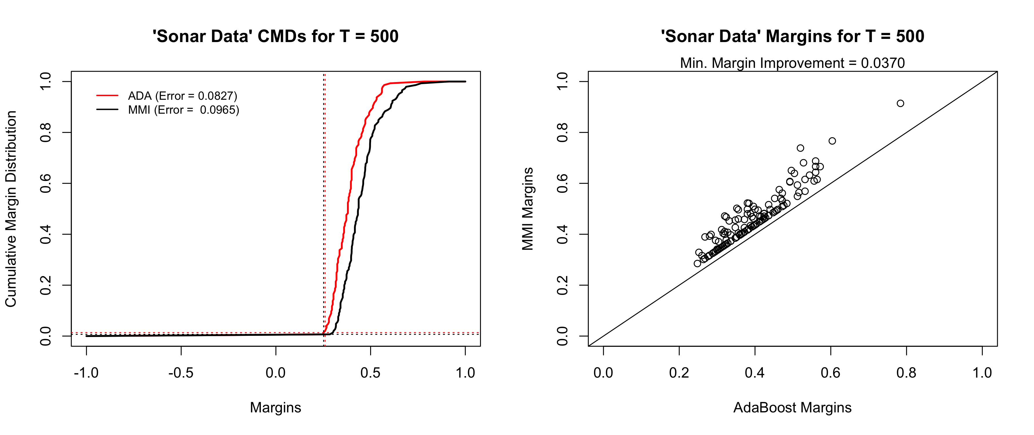
Figure 4: Comparison of AdaBoost and the MMI algorithm for the Ionosphere Data using 500 16-node (depth = 4) trees. The left panel compares the cumulative margin distributions (CMD) for AdaBoost and the MMI algorithm. The dotted lines indicate the Emargins (x-axis) and the Emargin Errors (y-axis). The right panel is a scatter plot of the AdaBoost margins and MMI margins. The line in the graph indicates equality of the margins.

Unlike Breiman’s arc-gv algorithm (Breiman, 1999), the MMI algorithm holds the complexity of the weak learners fixed by utilizing the same weak classifiers created by AdaBoost. We further guard against difference in complexities by restricting the analysis to a fixed depth with fixed number of terminal nodes (i.e., $k=4$ and depth = 2 in this example). The performance of the MMI algorithm in this particular example is ideal, considering it uses significantly fewer trees than the original AdaBoost solution, while improving upon the test set error rate. A generalization of this performance under different settings (i.e., different data sets, ensemble sizes, etc.) would strongly support the large margins theory and help us better design ensembles. Notwithstanding, we find that a better performance for the MMI algorithm is not always realized, and, in fact, the opposite is most often true. Consider, for example, Figure 4, which shows the performance of AdaBoost versus the MMI algorithm for the Australian Credit data set using 500 decision trees forced to have 16 terminal nodes ($k=16$, depth = 4). We note that all margin instances are higher than those of the original AdaBoost solution (the minimum margin improvement was 0.0302), yet the test set error rate for AdaBoost was better (0.1106) than that of the MMI algorithm (0.1442). The percentage of trees used by the MMI algorithm was also a fraction of the original as in the previous example, with only 94 out of the 500 trees with nonzero weights (just about 18.8% of the original weak classifiers). We also find this example contradicts the premise that a larger EMargin with lower EMargin Error should result in lower generalization performance contradicting the findings in Wang et al. (2011). The EMargin and EMargin error for the MMI algorithm are: $\hat{\theta}_{\text{ADA}}(q^{*})=0.2360$ with $q_{\text{ADA}}^{*}=0.5228$, while $\hat{\theta}_{\text{MMI}}(q^{*})=0.2834$ and $q_{\text{MMI}}^{*}=0.4066$. In other words, the EMargin for the MMI algorithm is higher with lower EMargin error.

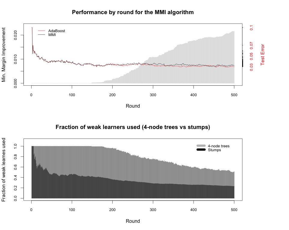
Figure 5: (Top Plot) By round comparison of AdaBoost and MMI algorithm for the Splice data set using decision trees with 4 terminal nodes (depth = 2). Lines indicate error rates and the density plot indicates minimum margin improvements. (Bottom Plot) Fraction of weak learners used for 4 terminal nodes (depth = 2) trees vs stumps (depth = 1).

In the previous examples we have found contradicting information regarding ensemble performance. We have empirically shown how it is possible to improve or maintain all of the margins in an ensemble solution by adjusting the weak classifier weights, yet have the same or worse test set performance. We have done this while keeping the complexity fixed. The lack of improvement in the test error rate contradicts the large margins theory, regardless of how “higher margins" is defined. Nevertheless, an example does not necessarily prove the theory is incorrect or incomplete. There are many questions unanswered including whether a better performance is only guaranteed in specific circumstances such as shallower trees, fewer iterations, or larger sample sizes. In the next section, we use simulation to find answers to these questions. We attempt to answer the question posed by Wang et al. (2011), which stated “can we find a strategy that optimizes the margin distribution? If such an algorithm exists, it would be a good test of our theory to see whether it has better performance than AdaBoost as we predict."

5 Experiments and Simulations

To further understand how the performance of the MMI algorithm changes as the number of weak learners increases, we plot the test set error rate for both the original AdaBoost solution and the MMI algorithm for $t=1,...,500$ on the Splice data set (see section 5 for description). The upper panel in Figure 5 shows that as the number of weak learners increases, the minimum margin improvement to the AdaBoost solution also increases. However the MMI algorithm does not outperform AdaBoost as the large margins theory suggest, in fact more often than not AdaBoost has a lower test set error rate. The lower panel on Figure 5 shows how the choice of tree depth affects the fraction of weak learners used given the number of weak learners combined. As the number of trees combined increases, the fraction of trees utilized decreases at a faster rate in stumps (depth = 1) when compared to 4-node (depth = 2) decision trees. This may be due to the fact that the LP solution more easily finds similarity in the stumps, as opposed to the 4-node (depth = 2) trees.

In Figure 6, we visualize the changes to the cumulative margin distributions for high values of $T=1000,5000$ and $10000$. As the number of weak learners combined increases, the minimum margin improvement (and consequently the average margin improvement) generally increases. It is evident for this particular data set that as $T$ increases, there is some amount of overfitting as the test set error degrades. In this particular case, the Emargin continues to increase, while the EMargin error decreases. It is worth mentioning that the bounds in (5), (LABEL:eq:7), (8) and (LABEL:eq:12) do not depend on $T$.

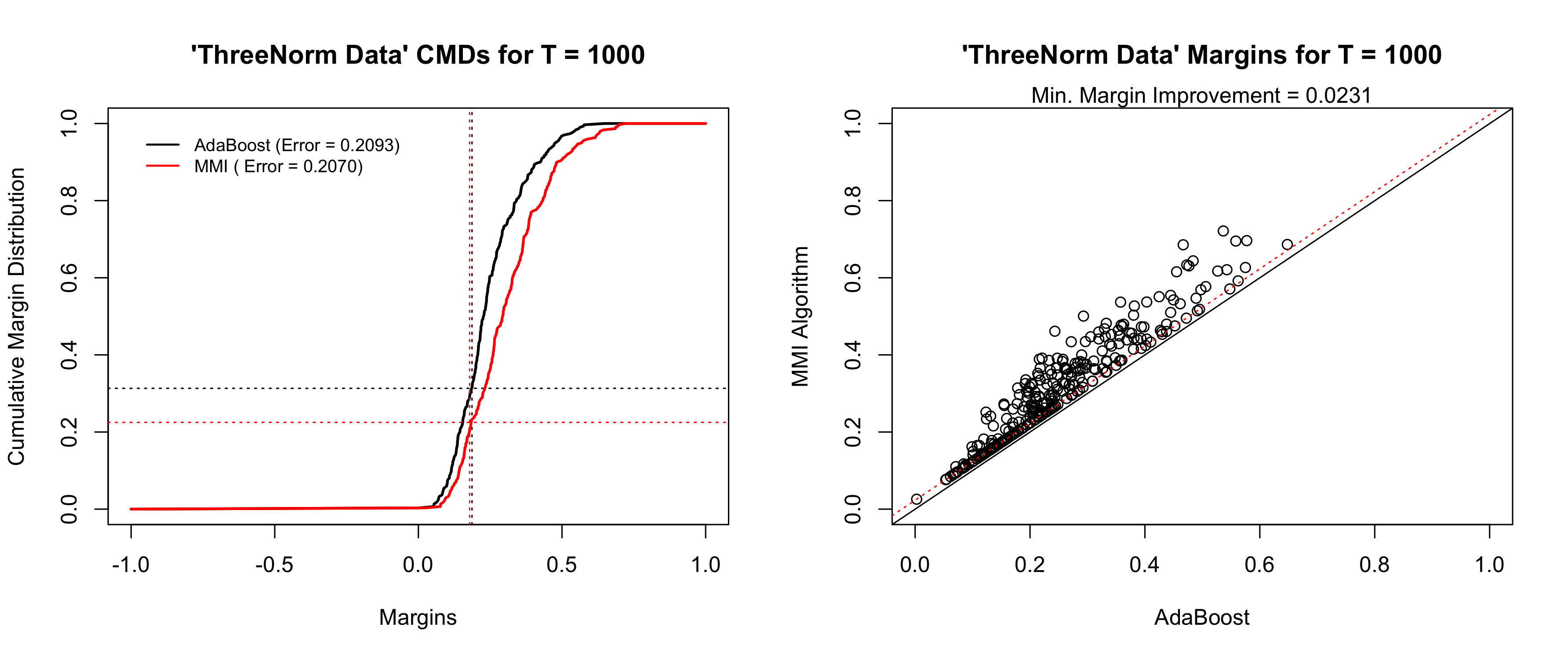
(a)

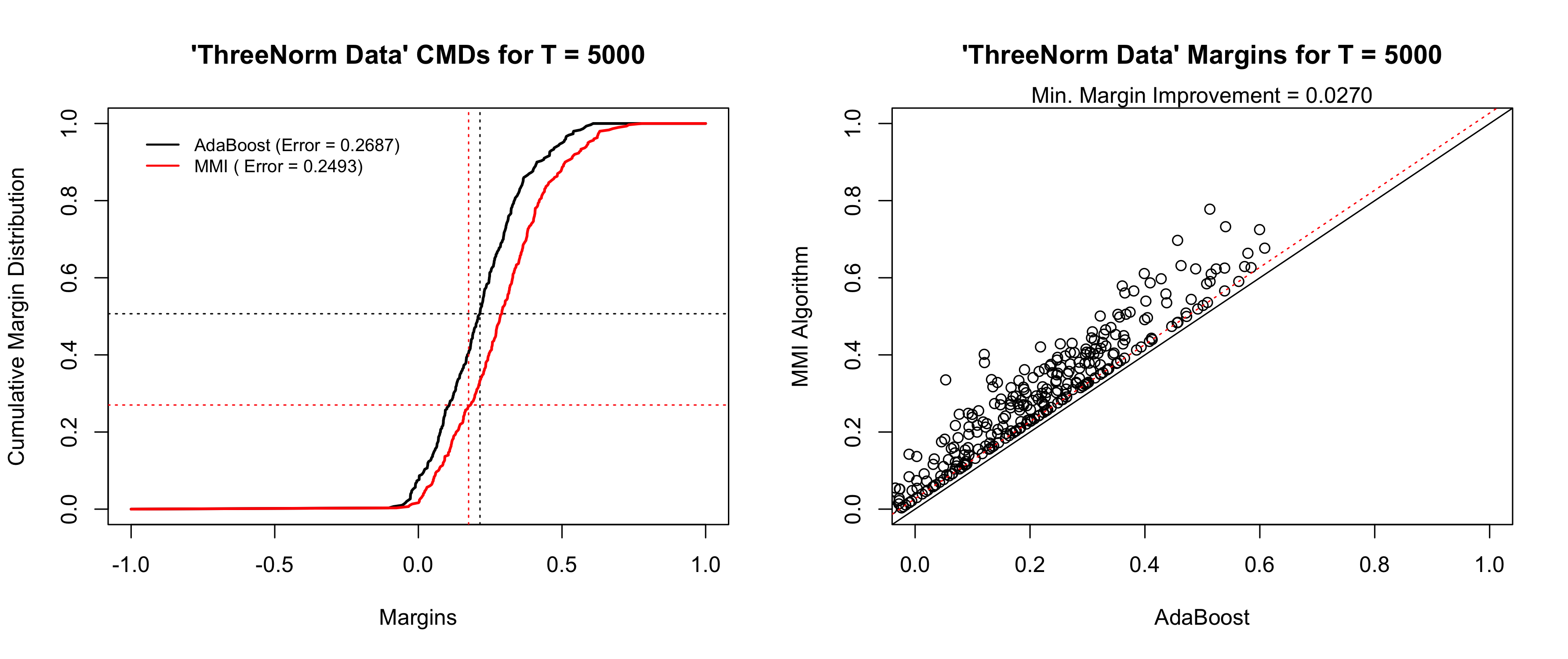
(b)

(c)

Figure 6: Cumulative margin distributions of AdaBoost versus the MMI Algorithm for the ThreeNorm Data for T = 1000, 5000, 10000 and corresponding margin scatter plots (right) of AdaBoost versus the MMI Algorithm.

We further test the proposed methods on 20 synthetic and real data sets (see Table 1 for descriptions of data sets). To fix the complexity, we only consider trees of depth = $\{1,2\}$, with $k=\{2,4\}$ respectively. We further normalize each feature to $\left[0,1\right]$ and consider 100 thresholds uniformly distributed on $\left[0,1\right]$ on each feature to be consistent with Wang et al. (2011), so that the $\mathscr{\left|H\right|}=2\times 100\times p$ for decision stumps and $\mathscr{\left|H\right|}=\left(2\times 100\times p\right)^{3}$ for 4-node (depth = 2) trees. The results are summarized in Tables 2, 3, 4, 5. Tables 2 and 3 illustrate the results for decision stumps using $T=\{250,500,750,1000\}$, while Tables 4 and 5 illustrate the results for 4-node (depth = 2) decision trees also using $T=\{250,500,750,1000\}$. We use a 70/30 sampling scheme for all data sets, except for those that already have a test set. We show the test set error rate, minimum margin improvement, average margin improvement, the EMargin and EMargin error for all data sets and experiments. Bold EMargins and EMargin errors indicate inconsistencies with the EMargin theory and the bound in (8) for Theorem 3. The results from using decision stumps indicate that the MMI algorithm cannot easily find optimized weights which improve upon the margin distribution resulting from the AdaBoost solution. Only when the number of combined classifiers $T$ is 750 and 1000 can we find changes in the margin distributions on specific data sets, such as the ColonCancer, Mushrooms, Musk, Sonar and TwoNorm data sets. For those simulations only the Sonar data set shows an improved performance, while the performance of the TwoNorm data set worsened and the rest of the data sets, even with improved margin distributions, have the same test set error performance. The results indicate that for 250 and 500 decision stumps, there is no difference in performance in terms of the test set error rate between AdaBoost and the MMI algorithm, and only two out of the 20 data sets had their margins distributions improved by MMI. For 750 and 1000 decision stumps, the AdaBoost algorithm performs better in one data set, while the MMI algorithm performed better in one data set. The rest of the data sets had exactly the same performance. The MMI algorithm was able to improve the margin distributions of six data sets. The greater improvements to the margins of data sets can be found using 4-node (depth = 2) trees. For instance 12 and 14 data sets had their margins distributions improved when $T=250$ and $T=500$ respectively. The AdaBoost algorithm performed better in 2 data sets out of 20, while the MMI algoritm performed better also in 2 out of the 20, while the rest were ties. AdaBoost performed better in 3 out of 20, while MMI performed better in 2 out of 20 using 500 decision trees. For 750 decision trees, virtually all data sets had improvements in their margins distributions, with AdaBoost outperforming MMI in 4 data sets, while MMI performed better in just 2. Surprisingly, for 1000 trees, MMI performed better in 6 data sets, while AdaBoost performed better in just 1.

Table 1: Description of Data Sets

Data Set	Description	Source	Training	Testing	Features
Australian	Credit Approval	Lichman (2013)	690		14
BreastCancer	Breast Cancer Wisconsin	Lichman (2013)	683		10
ColonCancer	Colon Cancer Data	Alon et al. (1999)	62		2000
Diabetes	Diabetes Patient Records	Lichman (2013)	768		8
FourClass	Non-Separable	Lichman (2013)	862		2
Gissette	Digit Recognition Data	Guyon et al. (2004)	6000	1000	5000
IJCNN1	IJCNN 2001 Competition	Prokhorov (2001)	49990	91701	22
Ionosphere	Ionosphere Data Set	Lichman (2013)	351		34
Madelon	Artificial Data	Guyon et al. (2004)	2000	600	500
Mushrooms	Mushrooms Data Set	Lichman (2013)	8124		112
Musk	Molecules Prediction	Lichman (2013)	6598		168
Parkinsons	Parkinsons Disease	Lichman (2013)	197		23
Pima	Pima Indians Data Set	Lichman (2013)	768		8
RingNorm	Breiman RingNorm	Lichman (2013)	210	90	20
Sonar	Sonar Data Set	Lichman (2013)	208		60
Spambase	Spam Emails Data Set	Lichman (2013)	4601		57
Splice	DNA Splice Junctions	Lichman (2013)	1000	2175	60
Transfusion	Blood Transfusion	Lichman (2013)	748		5
TwoNorm	Breiman TwoNorm	Lichman (2013)	300	3000	20
ThreeNorm	Breiman ThreeNorm	Lichman (2013)	300	3000	20

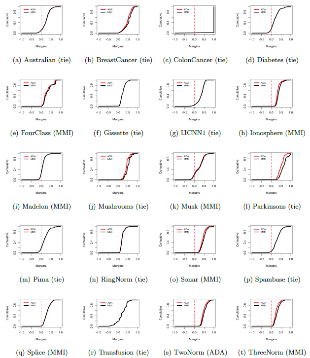
Figure 7: Cumulative Margin Distributions for AdaBoost vs the MMI algorithm using 1000 decision trees ($k=4$, depth = 2). In parenthesis, we can find which algorithm performed better.

Figure 7 illustrates visually the changes to the margin distributions obtained by the MMI algorithm for 1000 trees (4-node, depth = 2), in which the MMI algorithm outperformed AdaBoost in most data sets. It is not evident that the improvements to the margin distributions differed from other settings here.

Table 2: AB vs MMI Using Decision Stumps (MI = margin improvement, EM = EMargin).

		250 Trees ($k=2$, depth = 1)					500 Trees ($k=2$, depth = 1)
		Test Error	Min. MI	Avg. MI	EM	EM Error	Test Error	Min. MI	Avg. MI	EM	EM Error
Australian	AB	0.1106	-	-	0.3808	0.3776	0.1154	-	-	0.2854	0.3714
	MMI	0.1106	0.0000	0.0000	0.3808	0.3776	0.1154	0.0000	0.0000	0.2854	0.3714
BreastCancer	AB	0.0146	-	-	0.4040	0.1925	0.0195	-	-	0.3193	0.1778
	MMI	0.0146	0.0000	0.0000	0.4040	0.1925	0.0195	0.0000	0.0000	0.3193	0.1778
ColonCancer	AB	0.1579	-	-	0.5551	0.0232	0.1579	-	-	0.5667	0.0232
	MMI	0.1579	0.0001	0.0015	0.5551	0.0232	0.1579	0.0003	0.0016	0.5667	0.0232
Diabetes	AB	0.2511	-	-	0.2649	0.5177	0.2467	-	-	0.2302	0.5233
	MMI	0.2511	0.0000	0.0000	0.2649	0.5177	0.2467	0.0000	0.0000	0.2302	0.5233
FourClass	AB	0.2124	-	-	0.6979	0.7546	0.2085	-	-	0.5791	0.7546
	MMI	0.2124	0.0000	0.0000	0.6979	0.7546	0.2085	0.0000	0.0000	0.5791	0.7546
Gissette	AB	0.0419	-	-	0.2775	0.4354	0.0419	-	-	0.2738	0.5225
	MMI	0.0419	0.0000	0.0000	0.2775	0.4354	0.0419	0.0000	0.0000	0.2738	0.5225
IJCNN1	AB	0.1053	-	-	0.1862	0.1401	0.1083	-	-	0.1577	0.1475
	MMI	0.1053	0.0000	0.0000	0.1862	0.1401	0.1083	0.0000	0.0000	0.1577	0.1475
Ionosphere	AB	0.0755	-	-	0.3180	0.2980	0.0472	-	-	0.2140	0.2694
	MMI	0.0755	0.0000	0.0000	0.3180	0.2980	0.0472	0.0000	0.0000	0.2140	0.2694
Madelon	AB	0.4167	-	-	0.2050	0.6245	0.4100	-	-	0.1567	0.6700
	MMI	0.4167	0.0000	0.0000	0.2050	0.6245	0.4100	0.0000	0.0000	0.1567	0.6700
Mushrooms	AB	0.0172	-	-	0.2702	0.1081	0.0029	-	-	0.1709	0.0568
	MMI	0.0172	0.0000	0.0000	0.2702	0.1081	0.0029	0.0000	0.0000	0.1709	0.0568
Musk	AB	0.2238	-	-	0.2480	0.6723	0.1888	-	-	0.2191	0.7117
	MMI	0.2238	0.0000	0.0000	0.2480	0.6723	0.1888	0.0000	0.0000	0.2191	0.7117
Parkinsons	AB	0.1864	-	-	0.3360	0.3971	0.1525	-	-	0.2576	0.3162
	MMI	0.1864	0.0000	0.000	0.3360	0.3971	0.1695	0.0001	0.0067	0.2659	0.3529
Pima	AB	0.2511	-	-	0.2649	0.5177	0.2467	-	-	0.2302	0.5233
	MMI	0.2511	0.0000	0.0000	0.2649	0.5177	0.2467	0.0000	0.0000	0.2302	0.5233
RingNorm	AB	0.3180	-	-	0.1588	0.4667	0.2800	-	-	0.1262	0.4800
	MMI	0.3180	0.0000	0.0000	0.1588	0.4667	0.2800	0.0000	0.0000	0.1262	0.4800
Sonar	AB	0.2063	-	-	0.2342	0.4000	0.2222	-	-	0.2375	0.4759
	MMI	0.2063	0.0000	0.0000	0.2342	0.4000	0.2222	0.0000	0.0000	0.2375	0.4759
Spambase	AB	0.0681	-	-	0.1585	0.2189	0.0673	-	-	0.1772	0.2807
	MMI	0.0681	0.0000	0.0000	0.1585	0.2189	0.0673	0.0000	0.0000	0.1772	0.2807
Splice	AB	0.0818	-	-	0.1930	0.3240	0.0662	-	-	0.1561	0.3090
	MMI	0.0818	0.0000	0.0000	0.1930	0.3240	0.0662	0.0000	0.0000	01561	0.3090
Transfusion	AB	0.2133	-	-	0.3308	0.3174	0.2133	-	-	0.3917	0.3537
	MMI	0.2133	0.0000	0.0000	0.3308	0.3174	0.2133	0.0000	0.0000	0.3917	0.3537
TwoNorm	AB	0.0697	-	-	0.2246	0.2000	0.0677	-	-	0.1984	0.1667
	MMI	0.0697	0.0000	0.0000	0.2246	0.2000	0.0677	0.0000	0.0000	0.1984	0.1667
ThreeNorm	AB	0.2667	-	-	0.1826	0.5533	0.2473	-	-	0.1650	0.5700
	MMI	0.2667	0.0000	0.0000	0.1826	0.5533	0.2473	0.0000	0.0000	0.1650	0.5700
Summary
	AB	0 wins					0 wins
	MMI	0 wins					0 wins
		20 ties					20 ties

Table 3: AB vs MMI Using Decision Stumps (MI = margin improvement, EM = EMargin).

		750 Trees ($k=2$, depth = 1)					1000 Trees ($k=2$, depth = 1)
		Test Error	Min. MI	Avg. MI	EM	EM Error	Test Error	Min. MI	Avg. MI	EM	EM Error
Australian	AB	0.1154	-	-	0.2383	0.3714	0.1154	-	-	0.2276	0.3983
	MMI	0.1154	0.0000	0.0000	0.2383	0.3714	0.1154	0.0000	0.0000	0.2276	0.3983
BreastCancer	AB	0.0195	-	-	0.3122	0.2008	0.0195	-	-	0.2861	0.2008
	MMI	0.0195	0.0000	0.0000	0.3122	0.2008	0.0195	0.0000	0.0000	0.2861	0.2008
ColonCancer	AB	0.1579	-	-	0.5725	0.0233	0.1579	-	-	0.5752	0.0233
	MMI	0.1579	0.0004	0.0041	0.5725	0.0233	0.1579	0.0003	0.0031	0.5752	0.0233
Diabetes	AB	0.2511	-	-	0.2139	0.5456	0.2597	-	-	0.2041	0.5568
	MMI	0.2511	0.0000	0.0000	0.2139	0.5456	0.2597	0.0000	0.0000	0.2041	0.5568
FourClass	AB	0.1930	-	-	0.5096	0.7546	0.1930	-	-	0.5096	0.7546
	MMI	0.1930	0.0000	0.0000	0.5096	0.7546	0.1930	0.0000	0.0000	0.5096	0.7546
Gissette	AB	0.0419	-	-	0.2775	0.4354	0.0419	-	-	0.2738	0.5225
	MMI	0.0419	0.0000	0.0000	0.2775	0.4354	0.0419	0.0000	0.0000	0.2738	0.5225
IJCNN1	AB	0.1071	-	-	0.1374	0.1481	0.1079	-	-	0.1343	0.1584
	MMI	0.1071	0.0000	0.0000	0.1374	0.1481	0.1079	0.0000	0.0000	0.1343	0.1584
Ionosphere	AB	0.0566	-	-	0.1728	0.2490	0.0566	-	-	0.1847	0.3551
	MMI	0.0566	0.0000	0.0000	0.1728	0.2490	0.0566	0.0000	0.0000	0.1847	0.3551
Madelon	AB	0.2238	-	-	0.2480	0.6723	0.1888	-	-	0.2191	0.7117
	MMI	0.2238	0.0000	0.0000	0.2480	0.6723	0.1888	0.0000	0.0000	0.2191	0.7117
Mushrooms	AB	0.0028	-	-	0.1735	0.0556	0.0016	-	-	0.1673	0.0556
	MMI	0.0028	0.0000	0.0072	0.1735	0.0598	0.0016	0.0013	0.0062	0.1578	0.0492
Musk	AB	0.1538	-	-	0.1874	0.7087	0.1538	-	-	0.1604	0.6396
	MMI	0.1538	0.0000	0.0299	0.1874	0.7087	0.1538	0.0000	0.0315	0.2673	0.9429
Parkinsons	AB	0.1525	-	-	0.2762	0.4191	0.1525	-	-	0.2439	0.3823
	MMI	0.1525	0.0006	0.0086	0.2595	0.3971	0.1525	0.0013	0.0089	0.2460	0.3971
Pima	AB	0.2467	-	-	0.2302	0.5233	0.2597	-	-	0.2040	0.5568
	MMI	0.2467	0.0000	0.0000	0.2302	0.5233	0.2597	0.0000	0.0000	0.2040	0.5568
RingNorm	AB	0.2603	-	-	0.1188	0.4967	0.2433	-	-	0.1003	0.4033
	MMI	0.2603	0.0000	0.0000	0.1188	0.4967	0.2433	0.0000	0.0000	0.1003	0.4033
Sonar	AB	0.2222	-	-	0.2187	0.4759	0.2063	-	-	0.2029	0.4759
	MMI	0.1905	0.0010	0.0062	0.2103	0.4690	0.2063	0.0021	0.0114	0.1895	0.4483
Spambase	AB	0.0667	-	-	0.1616	0.2779	0.0637	-	-	0.1455	0.2689
	MMI	0.0667	0.0000	0.0000	0.1616	0.2779	0.0637	0.0000	0.0000	0.1455	0.2689
Splice	AB	0.0621	-	-	0.1685	0.3820	0.0607	-	-	0.1763	0.4310
	MMI	0.0621	0.0000	0.0000	0.1685	0.3820	0.0607	0.0000	0.0000	0.1763	0.4310
Transfusion	AB	0.2133	-	-	0.3803	0.3384	0.2133	-	-	0.3571	0.3155
	MMI	0.2133	0.0000	0.0000	0.3803	0.3384	0.2133	0.0000	0.0000	0.3571	0.3155
TwoNorm	AB	0.0647	-	-	0.1923	0.1600	0.0650	-	-	0.1874	0.1633
	MMI	0.0660	0.0000	0.0042	0.1939	0.1667	0.0653	0.0023	0.0100	0.2007	0.2100
ThreeNorm	AB	0.2350	-	-	0.1442	0.5100	0.2283	-	-	0.1472	0.5600
	MMI	0.2350	0.0000	0.0000	0.1442	0.5100	0.2283	0.0000	0.0000	0.1472	0.5600
Summary
	AB	1 wins					1 wins
	MMI	1 wins					1 wins
		18 ties					18 ties

Table 4: AB vs MMI Using 4-node (depth = 2) Trees (MI = margin improvement, EM = EMargin)

		250 Trees ($k=4$, depth = 2)					500 Trees ($k=4$, depth = 2)
		Test Error	Min. MI	Avg. MI	EM	EM Error	Test Error	Min. MI	Avg. MI	EM	EM Error
Australian	AB	0.1202	-	-	0.3151	0.3008	0.1202	-	-	0.2740	0.3361
	MMI	0.1202	0.0000	0.0026	0.3116	0.2987	0.1202	0.0000	0.0025	0.2740	0.3361
BreastCancer	AB	0.0098	-	-	0.3822	0.1611	0.0098	-	-	0.3147	0.1464
	MMI	0.0098	0.0027	0.0198	0.3738	0.1569	0.0098	0.0095	0.0380	0.2894	0.1297
ColonCancer	AB	0.1579	-	-	0.5725	0.0233	0.1579	-	-	0.5752	0.0233
	MMI	0.1579	0.0004	0.0041	0.5725	0.0233	0.1579	0.0003	0.0031	0.5752	0.0233
Diabetes	AB	0.2424	-	-	0.2793	0.4693	0.2424	-	-	0.2451	0.5065
	MMI	0.2424	0.0000	0.0004	0.2793	0.4693	0.2424	0.0000	0.0000	0.2451	0.5065
FourClass	AB	0.0656	-	-	0.2342	0.4461	0.0386	-	-	0.1805	0.3482
	MMI	0.0656	0.0000	0.0013	0.2342	0.4461	0.0386	0.0097	0.0312	02091	0.4146
Gissette	AB	0.0399	-	-	0.2365	0.4356	0.0399	-	-	0.2738	0.5225
	MMI	0.0399	0.0000	0.0000	0.2365	0.4356	0.0399	0.0000	0.0000	0.2778	0.5225
IJCNN1	AB	0.1010	-	-	0.1481	0.1071	0.1005	-	-	0.1420	0.1183
	MMI	0.1009	0.0000	0.0000	0.1482	0.1071	0.1005	0.0000	0.0000	0.1420	0.1183
Ionosphere	AB	0.0377	-	-	0.2849	0.1510	0.0566	-	-	0.2546	0.1102
	MMI	0.0377	0.0031	0.0127	0.2849	0.1510	0.0566	0.0184	0.0390	0.2373	0.0939
Madelon	AB	0.2238	-	-	0.2480	0.6723	0.1888	-	-	0.2191	0.7117
	MMI	0.2238	0.0000	0.0000	0.2480	0.6723	0.1888	0.0000	0.0000	0.2191	0.7117
Mushrooms	AB	0.0000	-	-	0.2464	0.0227	0.0000	-	-	0.2454	0.0260
	MMI	0.0000	0.0323	0.0617	0.1878	0.0188	0.0000	0.1601	0.1799	0.1604	0.0095
Musk	AB	0.1399	-	-	0.2365	0.4354	0.1818	-	-	0.2738	0.5225
	MMI	0.1399	0.0000	0.0002	0.2365	0.4354	0.1748	0.0022	0.0145	0.2778	0.5345
Parkinsons	AB	0.0678	-	-	0.3562	0.1250	0.0847	-	-	0.2855	0.0294
	MMI	0.0508	0.0558	0.1060	0.12803	0.0367	0.0678	0.0657	0.1238	0.2855	0.0294
Pima	AB	0.2424	-	-	0.2793	0.4693	0.2424	-	-	0.2451	0.5065
	MMI	0.2424	0.0000	0.0004	0.2793	0.4693	0.2424	0.0000	0.0000	0.2451	0.5065
RingNorm	AB	0.2090	-	-	0.1949	0.3233	0.1533	-	-	0.1528	0.2967
	MMI	0.2090	0.0000	0.0000	0.1949	0.3233	0.1533	0.0000	0.0001	0.1528	0.2967
Sonar	AB	0.1746	-	-	0.2659	0.0345	0.2063	-	-	0.2502	0.0207
	MMI	0.2063	0.0159	0.0359	0.2535	0.0275	0.2222	0.0206	0.0415	0.2390	0.0138
Spambase	AB	0.0637	-	-	0.1455	0.2689	0.0659	-	-	0.1916	0.2208
	MMI	0.0637	0.0000	0.0000	0.1455	0.2689	0.0659	0.0000	0.0001	0.1916	0.2208
Splice	AB	0.0336	-	-	0.2301	0.2260	0.0349	-	-	0.1899	0.2160
	MMI	0.0336	0.0000	0.0000	0.2301	0.2260	0.0349	0.0000	0.0000	0.1899	0.2160
Transfusion	AB	0.2133	-	-	0.3171	0.3575	0.2000	-	-	0.2590	0.3632
	MMI	0.2133	0.0000	0.0000	0.3171	0.3575	0.2000	0.0000	0.0000	0.2590	0.3632
TwoNorm	AB	0.0747	-	-	0.3078	0.0167	0.0613	-	-	0.2871	0.0133
	MMI	0.0827	0.0113	0.0287	0.2933	0.0133	0.0707	0.0244	0.0458	0.2871	0.0133
ThreeNorm	AB	0.2093	-	-	0.1982	0.2300	0.2030	-	-	0.1878	0.2400
	MMI	0.2063	0.0067	0.0000	0.2029	0.2533	0.2063	0.0153	0.0419	0.1797	0.2200
Summary
	AB	2 wins					3 wins
	MMI	2 wins					2 wins
		16 ties					15 ties

Table 5: AB vs MMI Using 4-node (depth = 2) Trees (MI = margin improvement, EM = EMargin)

		750 Trees ($k=4$, depth = 2)					1000 Trees ($k=4$, depth = 2)
		Test Error	Min. MI	Avg. MI	EM	EM Error	Test Error	Min. MI	Avg. MI	EM	EM Error
Australian	AB	0.1250	-	-	0.2610	0.3880	0.1250	-	-	0.2105	0.3589
	MMI	0.1250	0.0000	0.0021	0.2590	0.3860	0.1250	0.0000	0.0032	0.2053	0.3527
BreastCancer	AB	0.0098	-	-	0.2902	0.1485	0.0098	-	-	0.2912	0.1653
	MMI	0.0098	0.0126	0.0505	0.2778	0.1443	0.0098	0.0145	0.0560	0.2678	0.1506
ColonCancer	AB	0.1579	-	-	0.5725	0.0233	0.1579	-	-	0.5752	0.0233
	MMI	0.1579	0.0004	0.0041	0.5725	0.0233	0.1579	0.0003	0.0031	0.5752	0.0233
Diabetes	AB	0.2554	-	-	0.2431	0.5754	0.2424	-	-	0.2271	0.5978
	MMI	0.2554	0.0000	0.0004	0.2431	0.4754	0.2424	0.0000	0.0000	0.2271	0.5978
FourClass	AB	0.0154	-	-	0.1651	0.2935	0.0154	-	-	0.1426	0.1990
	MMI	0.0154	0.0126	0.0348	0.1690	0.3184	0.0116	0.0125	0.0328	0.1273	0.1426
Gissette	AB	0.0399	-	-	0.2365	0.4354	0.0218	-	-	0.2738	0.5225
	MMI	0.0399	0.0000	0.0000	0.2365	0.4354	0.0218	0.0000	0.0000	0.2738	0.5225
IJCNN1	AB	0.0999	-	-	0.1370	0.1229	0.1013	-	-	0.1259	0.1217
	MMI	0.1000	0.0000	0.0001	0.1370	0.1229	0.1013	0.0000	0.0000	0.1259	0.1217
Ionosphere	AB	0.0660	-	-	0.2164	0.0612	0.0660	-	-	0.2137	0.0531
	MMI	0.0600	0.0239	0.0526	0.2033	0.0449	0.0566	0.0292	0.0573	0.1943	0.0367
Madelon	AB	0.4167	-	-	0.2050	0.6245	0.3550	-	-	0.1252	0.6870
	MMI	0.4167	0.0000	0.0000	0.2050	0.6245	0.3600	0.0000	0.0001	0.1246	0.6860
Mushrooms	AB	0.0000	-	-	0.2385	0.0237	0.0000	-	-	0.1615	0.0058
	MMI	0.0000	0.0348	0.0768	0.1838	0.0128	0.0000	0.0351	0.0738	0.1646	0.0100
Musk	AB	0.2308	-	-	0.2536	0.4715	0.2797	-	-	0.2723	0.4835
	MMI	0.2308	0.0038	0.0149	0.2658	0.5015	0.2657	0.0048	0.0196	0.2835	0.5105
Parkinsons	AB	0.0847	-	-	0.2902	0.0368	0.0847	-	-	0.3439	0.1323
	MMI	0.0847	0.0639	0.1285	0.2902	0.0368	0.0847	0.0628	0.1270	0.2651	0.0294
Pima	AB	0.2554	-	-	0.2431	0.5754	0.2424	-	-	0.2271	0.5978
	MMI	0.2554	0.0000	0.0000	0.2431	0.5754	0.2424	0.0000	0.0000	0.2271	0.5978
RingNorm	AB	0.1260	-	-	0.1494	0.3633	0.1160	-	-	0.1323	0.3333
	MMI	0.1267	0.0000	0.0001	0.1494	0.3633	0.1160	0.0002	0.0030	0.1323	0.3633
Sonar	AB	0.2063	-	-	0.2689	0.1310	0.2063	-	-	0.2948	0.1241
	MMI	0.1746	0.0214	0.0496	0.2581	0.0827	0.1746	0.0213	0.0522	0.2498	0.0897
Spambase	AB	0.0637	-	-	0.1763	0.2317	0.0637	-	-	0.1570	0.2295
	MMI	0.0637	0.0000	0.0001	0.1757	0.2311	0.0637	0.0000	0.0000	0.1564	0.2292
Splice	AB	0.0377	-	-	0.1983	0.2620	0.0349	-	-	0.1853	0.2550
	MMI	0.0377	0.0000	0.0000	0.1983	0.2620	0.0340	0.0002	0.0052	0.1701	0.2240
Transfusion	AB	0.2000	-	-	0.2177	0.3671	0.1996	-	-	0.3000	0.5774
	MMI	0.2100	0.0000	0.0000	0.2177	0.3671	0.1996	0.0000	0.0000	0.3000	0.5774
TwoNorm	AB	0.0613	-	-	0.3131	0.0400	0.0590	-	-	0.2845	0.0200
	MMI	0.0673	0.0276	0.04811	0.2776	0.0133	0.0660	0.0276	0.0506	0.2845	0.0200
ThreeNorm	AB	0.2057	-	-	0.1984	0.3267	0.2093	-	-	0.1867	0.3133
	MMI	0.2050	0.0204	0.0589	0.1775	0.2633	0.2070	0.0231	0.0612	0.1784	0.2900
Summary
	AB	4 wins					1 wins
	MMI	2 wins					6 wins
		14 ties					13 ties

6 Conclusions

In the boosting literature, the upper bound on the generalization error in (3) developed by Schapire et al. (1998) led to the large margins theory, which suggests that, everything else being equal, larger margins should lead to better generalization error (see Schapire et al. 1998; Grove and Schuurmans 1998; Mason et al. 2000; Wang et al. 2011; Shen and Li 2010; Wang et al. 2011, 2012; Gao and Zhou 2013; Martinez and Gray 2014; Liu and Liao 2015; Zhang and Zhou 2016.) While the upper bound is theoretically correct, the large margins theory appears to be an over-interpretation of that result. The evidence presented in this paper shows that even if all of the margins are increased for a fixed set of weak learners, there is not necessarily an improvement in ensemble performance as measured by test set error, and in some cases the resulting ensemble performs worse. As Breiman (1999), Schapire et al. (1998) and Wang et al. (2011) have pointed out, the upper bounds presented in (3) and (4) are too loose to be practical, so that factors other than the margins may play a major role in generalization error. Based on the large margins theory, several researchers have attempted to directly optimize functions of the margins distribution  (Grove and Schuurmans, 1998; Breiman, 1999; Mason et al., 2000; Rätsch and Warmuth, 2002; Shen and Li, 2010; Zhou, 2014) and have met with mixed success in improving ensemble performance, but none of these algorithms is designed or guaranteed to increase or maintain all of the margins as the MMI algorithm does. This suggests that there may be special functions of margins, or even factors other than margins, that affect generalization error. We have shown that simply improving all of the margins for a fixed set of weak learners is not sufficient to improve generalization error. Although we do not rule out the importance of margins, we believe that there is room for other factors to influence the performance of boosting and other ensemble methods, and we conclude that the large margins theory, as currently stated, is insufficient in explaining the performance of ensemble methods.

References

- Alon et al. (1999) Alon, U., Barkai, N., Notterman, D. A., Gish, K., Ybarra, S., Mack, D., Levine, A. J., 1999. Broad patterns of gene expression revealed by clustering analysis of tumor and normal colon tissues probed by oligonucleotide arrays. Proceedings of the National Academy of Sciences 96 (12), 6745–6750.
- Breiman (1996a) Breiman, L., 1996a. Bagging predictors. Machine Learning 24 (2), 123–140.
- Breiman (1996b) Breiman, L., 1996b. Bias, variance, and arcing classifiers. Technical Report 460.
- Breiman (1999) Breiman, L., 1999. Prediction games and arcing algorithms. Neural Computation 11 (7), 1493–1517.
- Breiman (2000) Breiman, L., 2000. Special invited paper. additive logistic regression: A statistical view of boosting: Discussion. Annals of Statistics, 374–377.
- Breiman (2001) Breiman, L., 2001. Random forests. Machine Learning 45 (1), 5–32.
- Buja (2000) Buja, A., 2000. Additive logistic regression: A statistical view of boosting: Discussion. Annals of Statistics, 387–391.
- Chen and Guestrin (2016) Chen, T., Guestrin, C., 2016. Xgboost: A scalable tree boosting system. In: Proceedings of the 22nd acm sigkdd international conference on knowledge discovery and data mining. ACM, pp. 785–794.
- Cid (2012) Cid, W. G. M., 2012. Three essays on the use of margins to improve ensemble models. Ph.D. thesis, The University of Alabama.
- Coussement and De Bock (2013) Coussement, K., De Bock, K. W., 2013. Customer churn prediction in the online gambling industry: The beneficial effect of ensemble learning. Journal of Business Research 66 (9), 1629–1636.
- Dietterich (2000) Dietterich, T. G., 2000. Ensemble methods in machine learning. Multiple Classifier Systems, 1–15.
- Drucker and Cortes (1996) Drucker, H., Cortes, C., 1996. Boosting decision trees. Advances in Neural Information Processing Systems, 479–485.
- Drucker et al. (1994) Drucker, H., Cortes, C., Jackel, L., LeCun, Y., Vapnik, V., 1994. Boosting and other ensemble methods. Neural Computation 6 (6), 1289–1301.
- Freund (1995) Freund, Y., 1995. Boosting a weak learning algorithm by majority. Information and Computation 121 (2), 256–285.
- Freund and Schapire (1997) Freund, Y., Schapire, R. E., 1997. A decision-theoretic generalization of on-line learning and an application to boosting. Journal of Computer and System Sciences 55, 119–139.
- Friedman (2002) Friedman, J. H., 2002. Stochastic gradient boosting. Computational statistics & data analysis 38 (4), 367–378.
- Gao and Zhou (2013) Gao, W., Zhou, Z., 2013. On the doubt about margin explanation of boosting. Artificial Intelligence 203, 1–18.
- Graham (2015) Graham, B., 2015. Kaggle diabetic retinopathy detection competition report. University of Warwick.
- Grove and Schuurmans (1998) Grove, A. J., Schuurmans, D., 1998. Boosting in the limit: Maximizing the margin of learned ensembles. Proceedings of the Fifteenth National Conference on Artificial Intelligence, 692–699.
- Guyon et al. (2004) Guyon, I., Gunn, S., Ben-Hur, A., Dror, G., 2004. Result analysis of the nips 2003 feature selection challenge. In: Advances in Neural Information Processing Systems. pp. 545–552.
- Hoch (2015) Hoch, T., 2015. An ensemble learning approach for the kaggle taxi travel time prediction challenge. In: DC@ PKDD/ECML.
- Hong et al. (2014) Hong, T., Pinson, P., Fan, S., 2014. Global energy forecasting competition 2012.
- Kearns and Valiant (1994) Kearns, M., Valiant, L., 1994. Cryptographic limitations on learning boolean formulae and finite automata. Journal of the ACM (JACM) 41 (1), 67–95.
- King et al. (2014) King, M. A., Abrahams, A. S., Ragsdale, C. T., 2014. Ensemble methods for advanced skier days prediction. Expert Systems with Applications 41 (4), 1176–1188.
-
Lichman (2013)
Lichman, M., 2013. UCI machine learning repository.
URL http://archive.ics.uci.edu/ml - Liu and Liao (2015) Liu, C., Liao, S., 2015. Boosting via approaching optimal margin distribution. In: Pacific-Asia Conference on Knowledge Discovery and Data Mining. Springer, pp. 684–695.
- Long and Servedio (2010) Long, P. M., Servedio, R. A., 2010. Random classification noise defeats all convex potential boosters. Machine Learning 78 (3), 287–304.
- Lugosi and Vayatis (2004) Lugosi, G., Vayatis, N., 2004. On the bayes-risk consistency of regularized boosting methods. Annals of Statistics, 30–55.
- Maclin and Opitz (2011) Maclin, R., Opitz, D., 2011. Popular ensemble methods: An empirical study. Journal of Artificial Intelligence Research 11, 169–198.
- Martinez and Gray (2014) Martinez, W., Gray, J. B., 2014. The role of margins in boosting and ensemble performance. Wiley Interdisciplinary Reviews: Computational Statistics 6 (2), 124–131.
- Martinez and Gray (2016) Martinez, W., Gray, J. B., 2016. Noise peeling methods to improve boosting algorithms. Computational Statistics and Data Analysis 93, 483–497.
- Martinez and Gray (2019) Martinez, W., Gray, J. B., 2019. On the current state of research in explaining ensemble performance using margins.
- Mason et al. (2000) Mason, L., Bartlett, P. L., Baxter, J., 2000. Improved generalization through explicit optimization of margins. Machine Learning 38 (3), 243–255.
- Mease and Wyner (2008) Mease, D., Wyner, A., 2008. Evidence contrary to the statistical view of boosting. The Journal of Machine Learning Research 9, 131–156.
- Nielsen (2016) Nielsen, D., 2016. Tree boosting with xgboost-why does xgboost win" every" machine learning competition? Master’s thesis, NTNU.
- Opitz and Maclin (1999) Opitz, D., Maclin, R., 1999. Popular ensemble methods: An empirical study. Journal of Artificial Intelligence Research, 169–198.
- Prokhorov (2001) Prokhorov, D., 2001. Slide presentation in ijcnn’01, ford research laboratory. IJCNN.
- Puurula et al. (2014) Puurula, A., Read, J., Bifet, A., 2014. Kaggle lshtc4 winning solution. arXiv preprint arXiv:1405.0546.
- Quinlan (1996) Quinlan, J., 1996. Bagging, boosting, and c4. 5. AAAI/IAAI, Vol. 1, 725–730.
- Rätsch and Warmuth (2002) Rätsch, G., Warmuth, M. K., 2002. Maximizing the margin with boosting. Computational Learning Theory, 334–350.