Enabling Robust State Estimation through Measurement Error Covariance Adaptation

Abstract

Accurate platform localization is an integral component of most robotic systems. As these robotic systems become more ubiquitous, it is necessary to develop robust state estimation algorithms that are able to withstand novel and non-cooperative environments. When dealing with novel and non-cooperative environments, little is known a priori about the measurement error uncertainty, thus, there is a requirement that the uncertainty models of the localization algorithm be adaptive. Within this paper, we propose the batch covariance estimation technique, which enables robust state estimation through the iterative adaptation of the measurement uncertainty model. The adaptation of the measurement uncertainty model is granted through non-parametric clustering of the residuals, which enables the characterization of the measurement uncertainty via a Gaussian mixture model. The provided Gaussian mixture model can be utilized within any non-linear least squares optimization algorithm by approximately characterizing each observation with the sufficient statistics of the assigned cluster (i.e., each observation’s uncertainty model is updated based upon the assignment provided by the non-parametric clustering algorithm). The proposed algorithm is verified on several GNSS collected data sets, where it is shown that the proposed technique exhibits some advantages when compared to other robust estimation techniques when confronted with degraded data quality.

I Introduction

The applicability of robotic platforms to an ever increasing number of applications (e.g., disaster recovery [1], scientific investigations [2], health care [3]) has been realized in recent years. A core component that enables the operation of these platforms is the ability to localize (i.e., estimate the position states within a given coordinate frame) given a priori information and a set of measurements. Thus, a considerable amount of research has been afforded to the problem of accurate and robust localization of a robotic platform.

To facilitate the localization of a platform, a state estimation [4] scheme must be implemented. These state estimation frameworks can take two forms: either a batch estimator, or an incremental estimator. The batch variant of state estimation is generally facilitated through the utilization of a Nonlinear Least Squares (NLLS) algorithm (e.g., line-search method [5], or a trust-region method [6]). On the other hand, incremental state estimators are usually implemented as a variant of the Kalman filter [7] (e.g., the extended Kalman filter [8], or the unscented Kalman filter [9]).

The cost function underlying all of the state estimation techniques mentioned above is the $l^{2}$-norm of the estimation errors. This cost function enables accurate and efficient estimation when the assumed models precisely characterize the provided observations. However, when the utilized model does not accurately characterize the provided measurements, the estimation framework can provide an arbitrarily poor state estimate. Specifically, as discussed in [10], the $l^{2}$-norm cost function has an asymptotic breakdown of zero (i.e., if any single observation deviates from the utilized model, the estimated solution can be biased by an arbitrarily large quantity [11]).

To combat the poor breakdown properties of the $l^{2}$-norm cost function, several robust estimation frameworks have been proposed. These frameworks can be broadly partitioned into two categories: data weighting methods, and data exclusion methods. The data weighting methods work by iteratively calculating a measurement weighting vector such that observations which most substantially deviated form the utilized model have a reduced influence on the estimated result. Several commonly utilized data weight techniques include: robust Maximum Likelihood Estimators (m-estimators) [12], switchable constraints [13], dynamic covariance scaling (DCS) [14], and max mixtures [15]. On the other hand, the data exclusion methods work by finding a trusted subset of the provided observations. Several commonly utilized data exclusion techniques include: random sample consensus (RANSAC) [16], realizing, reversing, recovering (RRR) [17], $l^{1}$ relaxation [18], and receiver autonomous integrity monitoring (RAIM)[19].

Both estimation paradigms have certain undesirable properties. For example, in many applications, it is undesirable to completely remove observations that do not adhere to the defined model (e.g., the utilization of Global Navigation Satellite System (GNSS) in an urban environment where it may not be possible to estimate the desired states if observations are removed). Instead, it can be more informative to accurately characterize the measurement uncertainty model and accordingly reduce the observations influence on the estimate. This concept of data uncertainty model characterization naturally conforms to the data weighting class of robust techniques (as discussed more thoroughly in section II-A). However, the currently utilized weighting techniques have the undesirable property that they assume an accurate characterization of the true measurement uncertainty model can be provided a priori, which may not be a valid assumption if the robotic platform is operating in a novel environment.

Within this paper, we expand upon our prior work in [20] on a novel robust data weighting method, which relaxes the assumption that an accurate a priori measurement uncertainty characterization can be provided. This assumption is relaxed by iteratively estimating a Gaussian Mixture Model (GMM) based on the state estimation residuals that characterizes the measurement uncertainty model. This concept was also studied, following the work of [20], within [21] where an expectation-maximization (EM) clustering algorithm was implemented to characterize the measurement uncertainty model. The approach provided in this paper extends upon the work in [20] on two fronts: first, a computationally efficient variational approach [22, 23] is utilized for GMM model fitting as opposed to the collapsed Gibbs sampling [24] as previously utilized within [20], and secondly, the proposed approach is thoroughly verified on a diverse set of kinematically collected GNSS observations.

To facilitate a discussion of the proposed robust estimation technique, the remainder of this paper proceeds in the following manner. First, in Section II, an succinct overview of NLLS is provided, with a specific emphasis placed on robust estimation. In Section III, a novel robust estimation methodology, which enables adaptive observation de-weighting though the estimation of a multimodal measurement error covariance, is proposed. In Sections IV and V, the proposed approach is validated with multiple kinematic GNSS data-sets. Finally, the paper concludes with final remarks and proposed future research efforts.

II State Estimation

The traditional state estimation problem is concerned with finding the set of states, $X$, that, in some sense, best describe the set of observations, $Y$. An intuitive, and commonly utilized method to quantify the level of fit between the set of states and the set of observations is the evaluation of the posterior distribution, $\operatorname{p}(X\ |\ Y)$. When the state estimation problem is cast in this light, the desired set of states can be calculated through the maximization of the posterior distribution, as provided in Eq. 1, which is generally referred to as the maximum a posteriori (MAP) state estimate [4].

$$\hat{X}=\operatorname*{argmax}_{X}\ \operatorname{p}(X\ |\ Y)$$ (1)

A commonly utilized way to efficiently formulate the MAP estimation problem is through the application of the factor graph [25]. The factor graph enables efficient estimation through the factorization of the posterior distribution into the product of local functions (i.e., functions operating on a reduced domain when compared to the posterior distribution)

$$\operatorname{p}(X\ |\ Y)\propto\prod_{n=1}^{N}\psi_{i}(A_{n},B_{n}),$$ (2)

where, $A_{n}\subseteq\{X_{1},X_{2}\ldots,X_{n}\}$, and $B_{n}\subseteq\{Y_{1},Y_{2}\ldots Y_{m}\}$. It should be noted that the above expression could be an equality through multiplication by a normalization constant.

More formally, the factor graph is a bipartite graph with state nodes, $X$, and constraint nodes, $\psi$. Additionally, edges only exist between dependent state and constraint nodes [26]. This factorization is visually depicted in Fig. 1, for a simple GNSS example. Within Fig. 1, each $X$ represents a state vector to be estimated, and $\psi$ represents the constraints on a subset of the estimated states (e.g., $\psi_{n}$ could represent a GNSS pseudorange observation constraint on state vector $X_{n}$, or an inertial measurement linking two states together over time).

Figure 1: Example posterior distribution factorization with a factor graph for a GNSS example, where each $X_{n}$ represents a set of states to be estimated, and each $\psi_{n}$ represents a constraint on the associated (i.e., connected with an edge) state vectors.

Utilizing the factorization specified in Eq. 2 for the posterior distribution, the modified state estimation problem takes the form presented in Eq. 3.

$$\hat{X}=\operatorname*{argmax}_{X}\prod_{n=1}^{N}\psi_{n}(A_{n},B_{n})$$ (3)

In practice, this state estimation problem is simplified through the assumption that each factor adheres to a Gaussian uncertainty model (i.e., $\psi_{n}(A_{n},B_{n})\sim\mathscr{N}(\mu_{n},\Lambda_{n})$) [26]. When this assumption is enforced, the MAP estimation problem is equivalent to the minimization of the weighted sum of squared residuals [26], as provided in Eq. 4

$$\hat{X}=\operatorname*{argmin}_{X}\sum_{n=1}^{N}\lvert\lvert\ r_{n}(X)\ \rvert\rvert_{\Lambda_{n}}\quad\text{s.t.}\quad r_{n}(X)\triangleq y_{n}-h_{n}(X),$$ (4)

where, within this paper, the $\lvert\lvert\ *\ \rvert\rvert$ function is used to define the $l^{2}\text{-norm}$, $h_{n}$ is a mapping from the state space to the observation space, and $\Lambda_{n}$ is the provided symmetric, positive-semidefinite (PSD) covariance matrix , which is assumed to be diagonal.

With a cost function as presented in Eq. 4, a MAP state estimate can be calculated using any NLLS algorithm. To enable the selection of a NLLS algorithm, it is informative to coarsely partition the class of algorithms into two categories: line search techniques, and trust region techniques. The line search techniques operate by iteratively updating the previous state estimate by calculating a step direction $\Delta_{x_{k}}$ and a step magnitude, $\alpha_{k}$, (i.e., $\hat{X}_{k+1}=\hat{X}_{k}+\alpha_{k}\Delta_{x_{k}}$), where the specific calculation of $\alpha_{k}$, and $\Delta_{x_{k}}$ differs for varying algorithms (e.g., see the Gauss-Newton implementation [27] for one such example). The trust region based NLLS methods incorporate an additional constraint that the state update at the current iteration must fall within a ball of the current estimate (i.e., $||\alpha_{k}\Delta_{x_{k}}||<r$, where $r$ is the trust region radius). For trust region based methods, the Levenberg Marquardt [28] – which is the NLLS algorithm utilized within this study – and the Dog-leg [29] approaches are commonly utilized in practice.

II-A Robust State Estimation Through Covariance Adaptation

One of the major disadvantages of utilizing the $l^{2}\text{-norm}$ cost function is the undesirable asymptotic breakdown property [11]. Specifically, any estimator solely utilizing an $l^{2}\text{-norm}$ cost function will have an asymptotic breakdown point of zero. As discussed in [10], this property can be intuitively understood by letting any arbitrary observation, $y_{n}$, significantly deviate from the model (i.e., $\lvert\lvert y_{n}-h_{n}(X)\rvert\rvert_{\Lambda_{n}}\rightarrow\infty$), which, in turn, will arbitrarily bias the provided state estimate (i.e., $\lvert\lvert X\rvert\rvert\rightarrow\infty$).

The undesirable breakdown property of the $l^{2}\text{-norm}$ cost function has spurred significant research interest in the direction of robust state estimation [12, 13, 14, 15]. Within this paper, several of the major advances within the field will be discussed from the point-of-view of covariance adaptation; however, it should be noted that this is not an exhaustive compilation of all robust state estimation techniques. Rather, the purpose of this discussion is to provide a concise overview of the recent advances within the field, with specific emphasis placed on robust state estimation contributions now commonly adopted within the robotics community.

II-A1 M-Estimators

One of the initial frameworks developed to enable robust state estimation is through a class of m-estimators, as introduced by Huber [30, 12], that are less sensitive to erroneous observations than the $l^{2}$-norm. Specifically, this framework aims to replace the $l^{2}$-norm cost function, with a modified cost function that is more robust (i.e., increases more slowly when compared to the $l^{2}$-norm cost function, as depicted in Fig. 2). This class of modified cost functions, generically, take a form as presented in Eq. 5, where $\rho(*)$ is the modified cost function.

$$\hat{X} =\operatorname*{argmin}_{X}\sum_{n=1}^{N}\rho\big{(}\ \lvert\lvert r_{n}(X)\rvert\rvert_{\Lambda_{n}}\ \big{)}$$

$$=\operatorname*{argmin}_{X}\sum_{n=1}^{N}\rho(e_{n})\quad\text{s.t.}\quad e_{n}\triangleq\lvert\lvert r_{n}(X)\rvert\rvert_{\Lambda_{n}}$$ (5)

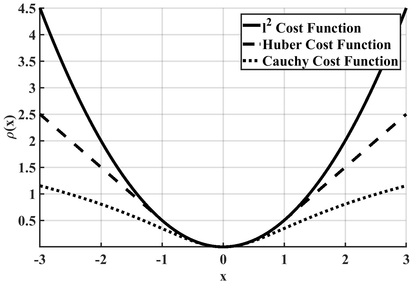
Figure 2: The cost function response for two commonly utilized robust m-estimators. Robust in this sense implies that the cost functions increases more slowly than the $l^{2}$-norm for large values of $x$. The specific form of the m-estimators is presented in Table I.

While numerous robust cost functions exist, we focus on two commonly utilized functions: the Huber and Cauchy cost functions. (For additional m-estimators, the reader is referred to [31].) Associated with each robust cost function is an influence and weighting function that can be used to enable these cost functions to be solved with the same NLLS approaches used for a quadratic cost function. A summary of the cost, influence and weight function is shown in Table I.

TABLE I: Functions utilized to implement the $l^{2}$-norm, Cauchy, and Huber cost functions, where, where $\rho(x)$ is the robust cost function, $\psi(x)\triangleq\frac{\partial\rho(x)}{\partial x}$ is the influence function, $w(x)\triangleq\frac{\psi(x)}{x}$ is the weighting function, and $k$ is the user defined kernel width.

M-Estimator	$\rho(x)$	$\psi(x)$	$w(x)$
$l^{2}\text{-norm}$	$x^{2}\mathbin{/}2$	$x$	$1$
Huber $\left\{\begin{array}[]{@{}ll@{}}\text{if}\ \ |x|\leq k\\ \text{if}\ \ |x|>k\end{array}\right.$	$\left\{\begin{array}[]{@{}ll@{}}\frac{1}{2}x^{2}\\ k(|x|-\frac{k}{2})\end{array}\right.$	$\left\{\begin{array}[]{@{}ll@{}}x\\ k\operatorname{sgn}(x)\end{array}\right.$	$\left\{\begin{array}[]{@{}ll@{}}1\\ k\mathbin{/}|x|\end{array}\right.$
Cauchy	$\frac{k^{2}}{2}log(1+\frac{x^{2}}{k^{2}})$	$x\mathbin{/}\big{[}1+x^{2}/k^{2}\big{]}$	$1\mathbin{/}\big{[}1+x^{2}/k^{2}\big{]}$

As discussed at the outset of this section, our objective is to view robust state estimation as a type of covariance adaptation. To view m-estimators as a type of covariance adaptation, we will begin by take the gradient of the modified cost function (see Eq. 5), as presented in Eq. 6.

$$\frac{\partial J}{\partial X} =\sum_{n=1}^{N}\frac{\partial\rho}{\partial e_{n}}\frac{\partial e_{n}}{\partial r_{n}}\frac{\partial r_{n}}{\partial X}$$

$$=r_{n}(X)^{T}\bigg{[}\frac{1}{e_{n}}\left.\frac{\partial\rho}{\partial e}\right|_{e_{n}(X)}\Lambda_{n}^{-1}\bigg{]}\frac{\partial r_{n}}{\partial X}.$$ (6)

The expression for the gradient of the modified cost function can be further reduced by noting that $\frac{1}{e_{n}}\frac{\partial\rho}{\partial e_{n}}$, is equivalent to the m-estimator weighting function, by definition. This simplifies the gradient expression for the m-estimators cost function as presented in Eq. 7, which is equivalent to the traditional $l^{2}$-norm cost function, but with an adaptive covariance. The modified covariance, $\hat{\Lambda}_{n}$, is provided in Eq. 8, where the specific weighting function is dependent upon the utilized m-estimator.

$$\frac{\partial J}{\partial X}=r_{n}(X)^{T}\bigg{[}w\big{(}e_{n}\big{)}\Lambda_{n}^{-1}\bigg{]}\frac{\partial r_{n}}{\partial X},$$ (7)

$$\hat{\Lambda}_{n}=\big{[}w(e_{n})\Lambda_{j}^{-1}\big{]}^{-1}=\frac{1}{w(e_{n})}\Lambda_{j},$$ (8)

From this discussion, it should be noted that the robust state estimation problem when m-estimators are utilized is equivalent to an iteratively re-weighted least squares (IRLS) problem [32, 33]. In IRLS, the effect of an erroneous observation is minimized by covariance adaptation based on the previous optimization iteration’s residuals, as presented in Eq. 9. The equivalence between m-estimators and IRLS has been previously noted in the literature [34, 35].

$$\hat{X}=\operatorname*{argmin}_{X}\sum_{n=1}^{N}w_{n}(e_{n})\ \lvert\lvert\ r_{n}(X)\ \rvert\rvert_{\Lambda_{n}}$$ (9)

II-A2 Switch Constraints

A more recent advancement within the robotics community, switch constraints (as introduced in [36]) is a specific realization of a lifted state estimation scheme [37]. Switch constraints augment the optimization problem by concurrently solving for the desired states and a set of measurement weighting values, as provided in Eq. 10

$$\hat{X},\hat{S}=\operatorname*{argmin}_{X,S}\sum_{n=1}^{N}\bigg{[}\lvert\lvert\ \psi(s_{n})r_{n}(X)\ \rvert\rvert_{\Lambda_{n}}+||\ \gamma_{n}-s_{n}\ ||_{\Xi_{n}}\bigg{]},$$ (10)

where $S$ is the set of estimated measurement weights, $\psi()$ is a real-valued function such that $\psi(*)\rightarrow[0,1]$, and $\gamma$ is a prior on the switch constraint.

To explicitly view the switch constraint technique as a covariance adaptation method, we can evaluate the effect that switchable constraints will have on measurement constraint in the modified cost function (e.g., Eq. 10), as depicted in Eq. 11 where $w_{n}\triangleq\psi(s_{n})$. This relation can be further reduced to the expression presented in Eq. 12, where $\hat{\Lambda}_{n}^{-1}=w_{n}^{2}\Lambda_{n}^{-1}$, by noting that $w_{n}$ is a scalar.

$$||\ \psi(s_{n})r_{n}(X)\ ||_{\Lambda_{n}} =\big{[}w_{n}r_{n}(X)\big{]}^{T}\Lambda^{-1}_{n}\big{[}w_{n}r_{n}(X)\big{]}$$ (11)

$$=r_{n}(X)^{T}\hat{\Lambda}_{n}^{-1}r_{n}(X)$$ (12)

The relation presented in Eq. 12 directly shows a relation between the estimated observation weighting — as implemented in the switchable constraint framework — and the scaling of the a priori measurement covariance matrix.

II-A3 Dynamic Covariance Scaling

One potential disadvantage of the switchable constraint framework is the possibility for an increased convergence time due to the augmentation of the optimization space [14]. To combat this issue, the DCS [14] approach was proposed as a closed-form solution to the switch constraint weighting optimization. The m-estimator equivalent weighting function, as derived within [38], is provided as

$$w\big{(}x\big{)}=\begin{cases}1,&\text{if $x^{2}\leq k$}.\vspace{0.5em}\\ \frac{4k^{2}}{(x^{2}+k)^{2}},&\text{otherwise},\end{cases}$$ (13)

where $k$ is the user defined kernel width, which dictates the residual threshold for observations to be considered erroneous. From this expression, it is noted that DCS is equivalent to the standard least-squares estimator when the residuals are less than the kernel width $k$; however, when residuals lie outside of the kernel width, the corresponding observations are de-weighted according to the provided expression.

From the provided weighting expression, the equivalent DCS robust m-estimator can be constructed, as presented in Table II. This is performed by utilizing the definitions provided within [34], (i.e., assuming a weighting function is provided, then the influence function is calculated as $\psi(x)=x\ w(x)$ and the robust cost function is $\rho(x)=\int\psi(x)dx$).

TABLE II: Equivalent dynamic covariance scaling m-estimator, $w(x)$ is the weighting function – as specified in Eq. 13, $\psi(X)\triangleq x\ w(x)$ is the influence function, $\rho(X)=\int\psi(x)dx$ is the robust cost function, and $k$ is the user defined kernel width.

M-Estimator	$\rho(x)$	$\psi(x)$	$w(x)$
DCS $\left\{\begin{array}[]{@{}ll@{}}\text{if}\ \ x^{2}\leq k\\ \text{if}\ \ x^{2}>k\end{array}\right.$	$\left\{\begin{array}[]{@{}ll@{}}\frac{1}{2}x^{2}\\ \frac{k\big{(}3x^{2}-k\big{)}}{2\big{(}x^{2}+k\big{)}}\end{array}\right.$	$\left\{\begin{array}[]{@{}ll@{}}x\\ \frac{4k^{2}x}{(x^{2}+k)^{2}}\end{array}\right.$	$\left\{\begin{array}[]{@{}ll@{}}1\\ \frac{4k^{2}}{(x^{2}+k)^{2}}\end{array}\right.$

With the DCS equivalent m-estimator, and the discussion provided in section II-A1, it can seen that DCS based state estimation enables robustness through the adaptation of the a priori measurement error covariance. The specific relation between the a priori and modified covariance matrices is provided in Eq. 8 with a weighting function implementation as provided in Eq. 13.

II-A4 Max Mixtures

While the previously discussed estimation frameworks do enable robust inference, they still have the undesirable property that the measurement uncertainty model must adhere to a uni-modal Gaussian model. To relax this assumption, a GMM [39] can be utilized to represent the measurement uncertainty model. The GMM characterizes the uncertainty model as a weighted sum of Gaussian components, as depicted in Eq. 14, where $r_{n}\triangleq y_{n}-h_{n}(X)$ is an observation residual, $w=\{w_{1},w_{2},\ldots,w_{m}\}$ is the set of mixture weights with the constraint that $\sum_{m=1}^{M}w_{m}=1$, and $\mu_{m}$, $\Lambda_{m}$ are the mixture component mean and covariance, respectively.

$$r_{n}\sim\sum_{m=1}^{M}w_{m}\mathscr{N}(r_{n}\ |\ \mu_{m},\Lambda_{m})$$ (14)

Utilizing a GMM representation of the measurement uncertainty model can greatly increase the accuracy of the measurement error characterization; however, it also greatly increases the complexity of the optimization problem. This increase in complexity is caused by the inability to reduce the factorization presented in Eq. 3 to a NLLS formulation, as was possible when a uni-modal Gaussian model was assumed.

To enable the utilization of a GMM while minimizing the computational complexity of the optimization process, the max-mixtures approach was proposed within [15]. This approach circumvents the increased computational complexity by replacing the summation operation in the GMM with the maximum operation, as depicted in Eq. 15, where $\mathrel{\dot{\sim}}$ depicts that $r_{n}$ is approximately distributed according to the right-hand side.

$$r_{n}\mathrel{\dot{\sim}}\max_{m}w_{m}\mathscr{N}(r_{n}\ |\ \mu_{m},\Lambda_{m})$$ (15)

Within Eq. 15, the maximum operator acts as a selector (i.e., for each observation, the maximum operator selects the single Gaussian component from the GMM that maximizes the likelihood of the individual observation given the current state estimate). Through this process, each observation is only utilizing the single Gaussian component from the model, which allows for the simplification of the optimization process to the weighted sum of squared residuals [40, 26] (i.e., a NLLS optimization problem).

Similar to the previously discussed robust state estimation formulations, the max-mixtures implementation can also be interpreted as enabling robustness through covariance adaptation. Where, the covariance adaptation is enabled through the maximum operator. Specifically, each observation initially belongs to a single component from the GMM model, then through the iterative optimization process, the measurement error covariance for each observation is updated to one of the components from within the predefined GMM.

III Proposed Approach

As shown by the discussion in section II, several robust state estimation frameworks have been proposed. Each of the discussed estimators work under the assumption that an accurate a priori measurement error covariance is available. However, in practice, the requirement to supply an accurate a priori characterization of the measurement uncertainty model is not always feasible when considering that the platform could be operating in a novel environment, a non-cooperative environment, or both.

Within this section, the batch covariance estimation (BCE) framework is proposed to address the issue of robust state estimation where, the framework is not only robust to erroneous observations, but also erroneous a priori measurement uncertainty estimates. To elaborate on the BCE framework, the remainder of this section proceeds in the following manner: first, the assumed data model is discussed; then, a method for learning the measurement error uncertainty model from residuals is provided; finally, the BCE framework is described.

III-A Data Model

Given a set of residuals $R=\{r_{1},r_{2},\ldots,r_{n}\}$ with $r_{n}=y_{n}-h_{n}(X)\in\mathbb{R}^{d}$. We will assume that the set can be partitioned into groupings of similar residuals (i.e., $\bigcup_{m=1}^{M}C_{m}=R$), where each group, $C_{k}$, can be fully characterized by a Gaussian distribution (i.e., $C_{k}\sim\mathscr{N}(\mu_{k},\Lambda_{k})$). Given this assumptions, the set of residuals are fully characterized as a weighted sum of Gaussian distributions (i.e., a GMM), as depicted in Eq. 16

$$r_{n}\sim\sum_{m=1}^{M}w_{m}\mathscr{N}(r_{n}\ |\ \theta_{m})\quad\text{s.t.}\quad\theta_{m}\triangleq\{\mu_{m},\Lambda_{m}\},$$ (16)

where, $w$ is the set of mixture weights with the constraint that $\sum_{m}w_{m}=1$, and $\theta_{m}$, is the mixture components sufficient statistics (i.e., the mixture component mean and covariance).

To enable the explicit assignment of each data point to a Gaussian component within the GMM, an additional latent parameter, $Z=\{z_{1},z_{2},\ldots,z_{n}\}$ with $z_{n}\in\mathbb{R}^{M}$, is incorporated. The assignment variables $Z$ are characterized according to a categorical distribution, as depicted in Eq. 17, where $w_{m}$ is the component weight, and $\operatorname{I}_{[*]}$ is the indicator function which evaluates to 1 if the equality within the brackets is true and 0 otherwise.

$$\operatorname{p}(z_{n}\ |\ w)=\prod_{m=1}^{M}w_{m}\operatorname{I}_{[z_{n}=m]}$$ (17)

Through the incorporation of the categorically distributed assignment parameters into the GMM, every data instance $r_{n}\in R$ can be characterized through Eq. 18. Where, this equation explicitly encodes that each data instance is characterized by a single Gaussian component from the full GMM.

$$\operatorname{p}(r_{n}\ |\ \theta_{m},z_{m})=\sum_{m=1}^{M}w_{m}\mathscr{N}(r_{n}\ |\ \theta_{m})\operatorname{I}_{[z_{n}=m]}$$ (18)

As a Bayesian framework will be utilized for model fitting (as described in section III-B), a prior distribution must be defined for the GMM mixture weights $w$, and the sufficient statistics, $\theta$. To define the prior over the mixture weights, $w$, a Dirichlet distribution [41] is utilized, as it is a conjugate prior to the categorical distribution [43]. The specific form of the Dirichlet prior is provided in Eq. 19, where $\alpha=(\alpha_{1},\ldots,\alpha_{k})$ is a set of hyper-parameters such that $\alpha_{i}>0$, and $S$ is the probability simplex.

$$\operatorname{p}(w|\alpha)=\frac{\Gamma(\sum_{m=1}^{M}(\alpha_{M}))}{\prod_{m=1}^{M}(\Gamma(\alpha_{m}))}\prod_{m=1}^{M}w_{m}^{\alpha_{i}-1}\operatorname{I}_{[w_{m}\in S]}$$ (19)

To define a prior over the GMM sufficient statistics, $\theta$, the normal inverse Wishart (NIW) is utilized due to the conjugate relation with the multivariate Gaussian that has unknown mean and covariance [44]. The NIW distribution is defined in Eq. 20, where $\beta=\{m_{o},\kappa_{o},\nu_{o},S_{o}\}$ is the set of hyper-parameters, and $\operatorname{W}^{-1}$ is the inverse Wishart distribution, as discussed within [45], where $\Gamma_{d}(*)$ is the multivariate gamma function, $\operatorname{Tr}(*)$ is the matrix trace, and $d$ is the dimension of $S_{o}$.

$$\operatorname{p}(\theta \ |\ \beta)=\ \mathscr{N}(\mu|m_{o},\frac{1}{\kappa_{o}}\Lambda)\operatorname{W}^{-1}(\Lambda|S_{o},\nu_{o})$$ (20)

$$\ \text{s.t.}\ \operatorname{W}^{-1}(\Lambda\ |\ S_{o},\nu_{o})=\frac{\lvert\Lambda\rvert^{\frac{\nu_{o}-d-1}{2}}}{2^{\nu_{o}\frac{d}{2}}\ {\Gamma_{d}\big{(}\frac{\nu_{o}}{2}\big{)}\ \lvert S_{o}\rvert^{\frac{\nu_{o}}{2}}}}e^{-\frac{1}{2}\operatorname{Tr}\big{(}S_{o}^{-1}\Lambda\big{)}}$$

Utilizing the data model defined earlier, the joint probability distribution that characterizes the system is defined in Eq. 21. Additionally, a visual representation of the underlying model is graphically represented in Fig. 3.

$$\operatorname{p}(R,\theta,Z)= \operatorname{p}(w\ |\ \alpha)\cdot$$

$$\prod_{n=1}^{N}\operatorname{p}(z_{n}\ |\ w_{n})\operatorname{p}(r_{n}\ |\ z_{n},\theta)\cdot$$

$$\prod_{m=1}^{M}\operatorname{p}(\theta_{m}\ |\ \beta)$$ (21)

Figure 3: Graphical representation of the utilized data model which visually encodes the joint probability distribution presented in Eq. 21. Each red node represents a latent parameter, and the blue node represents the provided observations. The plate notation [46] is utilized to represent the replication of a random variable.

III-B Gaussian Mixture Model Fitting

Provided with the joint distribution, as depicted in Eq. 21, the ultimate goal of a GMM fitting algorithm is to estimate the model parameters that maximize the $\operatorname{log\ marginal\ likelihood}$, as provided in Eq. 22, of the observations [39, 23]. Due to the dimensionality of the space, the integral presented in Eq. 22 is not computational tractable in general [47]. Thus, techniques for approximating the integral need to be utilized.

$$\operatorname{log}\operatorname{p}(R)=\operatorname{log}\int\operatorname{p}(R,\theta,Z)d\mathbf{Z}d\boldsymbol{\theta}$$ (22)

In practice, two broad classes of integral approximation algorithms are utilized: Monte Carlo methods [48], and variational methods [49]. The Monte Carlo methods approximate the integral by averaging the response of the integrand for a finite number of samples. In contrast, the variational approaches convert from an integration into an optimization problem, by defining a family of simplified functions (i.e., the family of exponential probability distributions) and optimizing the function within that family that most closely matches the original function [49].

Within this work, it was elected to utilize a variational model fitting approach, as this class of algorithms dramatically reduce the computational complexity of the problem when compared to Monte Carlo techniques [47]. To implement this approach, for the proposed data model, the assumption is made that the joint distribution defined in Eq. 21 can be represented as, $\operatorname{p}(R,\theta,Z)\approx\operatorname{q}(\theta)\operatorname{q}(Z)$, which is commonly referred to as the mean-field approximation [49]. Utilizing the mean-field approximation, the $\operatorname{log\ marginal\ likelihood}$ is represented as Eq. 23. Through the application of Jensens’s inequality [50], the equality in Eq. 23 can be converted into a lower bound on the $\operatorname{log\ marginal\ likelihood}$, as presented in Eq. 24.

$$\operatorname{log}\operatorname{p}(R) =\operatorname{log}\int\operatorname{q}(Z)\operatorname{q}(\theta)\frac{\operatorname{p}(R,\theta,Z)}{\operatorname{q}(Z)\operatorname{q}(\theta)}dZd\theta$$ (23)

$$\begin{aligned} \ \ \geq&\int\operatorname{q}(Z)\operatorname{q}(\theta)\operatorname{log}\frac{p(R,Z\ |\ \theta)}{\operatorname{q}(Z)}dZd\theta\ +\\ &\int\operatorname{q}(\theta)\operatorname{log}\frac{\operatorname{p}(\theta)}{\operatorname{q}(\theta)}d\theta\end{aligned}$$ (24)

The right hand side of the inequality presented in Eq. 24 is commonly referred as the free energy functional [23], as depicted in Eq. 25. As it is a lower bound on the $\operatorname{log\ marginal\ likelihood}$, an optimal set of model parameters can be found through iterative optimization.

$$\operatorname{log}\operatorname{p}(R)\geq\operatorname{F}\big{[}\operatorname{q}(Z),\operatorname{q}(\theta)\big{]}$$ (25)

To find the set of equations necessary for iterative parameter optimization, the partial derivative of the free energy function can be taken with respect to $\operatorname{q}(Z)$, and $\operatorname{q}(\theta)$. When the partial derivative of the free energy functional is taken with respect to $\operatorname{q}(Z)$, as presented in Eq. 26, the latent parameters, $Z$, can be updated by holding the model parameters, $\theta$, fixed and optimizing for $Z$. Likewise, when the partial derivative of the free energy functional is taken with respect to $\operatorname{q}(\theta)$, as presented in Eq. 27, the model parameters, $\theta$, can be updated by holding the latent parameters, $Z$, fixed and optimizing for $\theta$. Within Eq. 26 and Eq. 27 the terms $C_{z}$ and $C_{\theta}$ are normalizing constants for $\operatorname{q}(Z)$ and $\operatorname{q}(\theta)$, respectively.

$$\operatorname{q}(z)_{t+1}=C_{z}\int\operatorname{q}(\theta)_{t}\operatorname{log}p(R,Z\ |\ \theta)d\theta$$ (26)

$$\operatorname{q}(\theta)_{t+1}=C_{\theta}\operatorname{p}(\theta)\int\operatorname{q}(Z)_{t+1}\operatorname{log}\operatorname{p}(R,Z\ |\ \theta)dZ$$ (27)

When the variantional inference framework, as summarized in Eq. 26 and Eq. 27, is provided with a data set, $R$, which conforms to the models discussed in section III-A, the output is a GMM which characterizes the underlying probability distribution. Within this paper, the GMM will be utilized to provide an adaptive characterization of the measurement uncertainty model.

III-C Algorithm Overview

Multiple robust state estimation frameworks have been developed, as discussed in section II. However, it was noted that all of the discussed approaches fall short on at least one front. The primary shortcoming shared by all the approaches is the inability to provide an accurate state estimate when provided with an inaccurate a priori measurement error uncertainty model. To confront this concern, a novel IRLS formulation is proposed within this section.

The proposed BCE approach is graphically depicted in Fig. 4, where it is shown that the algorithm is composed of two sections: the initialization, and the robust iteration. To initialize the algorithm, a factor graph is constructed given the a priori state and uncertainty information and the set of measurements. Utilizing the constructed factor graph, an initial iteration of the NLLS optimizer is used to update the state estimate and calculate a set of measurement residuals.

With the residuals from the initial iteration of the NLLS optimizer, the algorithm proceeds into the first robust iteration step. Each robust iteration step commences with the generation of a GMM that characterizes the measurement uncertainty through the variational inference framework discussed in section III-B, operating on the most recently calculated set of residuals. With the provided GMM, the measurement uncertainty model of the factor graph is updated (i.e., each measurement’s uncertainty model is updated based upon the sufficient statistics of the assigned cluster from the GMM). Finally, the state estimate is updated by feeding the modified factor graph into the NLLS optimization algorithm. This robust iteration scheme is iterated until a measure of convergence – or the maximum number of iterations – has been reached.

Because this framework iteratively updates a GMM based measurement uncertainty model, the proposed approach is not only robust to erroneous measurements, but also robust to poor estimates of the a priori measurement uncertainty model.

Figure 4: Schematical overview of the proposed batch covariance estimation algorithm. The proposed approach enables robust state estimation through the iterative estimation of the – possible multimodal – measurement error covariance model, where the measurement error covariance model is characterized by a Gaussian mixture model that is fit to the residuals of the previous iteration of optimization.

IV Experimental Setup

IV-A Data Collection

To demonstrate the capabilities of our robust optimization framework, we evaluate our system using Global Positioning System (GPS) signals from a variety of environments, including open-air, and urban terrain. Due to the varying environments, the measurement uncertainty for each GPS measurements is unknown a priori and differs over time. Furthermore, using different qualities of GPS receivers also leads to differing measurement uncertainties.

To test the proposed estimation approach using actual degraded GPS observables, binary In-phase and Quadrature (IQ) data in the L1-band was recorded using a LabSat-3 GPS record and playback device [52] during three kinematic driving tests, as depicted in Fig. 5, in the Morgantown, WV area. These IQ data were then played back into both a geodetic-grade GNSS receiver (Novatel OEM-638) and an open-source GPS software defined radio (SDR), the GNSS-SDR library [53]. With this experimental setup, the geodetic-grade GNSS receiver was treated as a baseline reference for the best achievable GPS observable quality, and the GPS SDR was used to tune the quality of the observables to two different levels of performance ranging from low-grade to high-grade (i.e, close to matching the reference receiver).

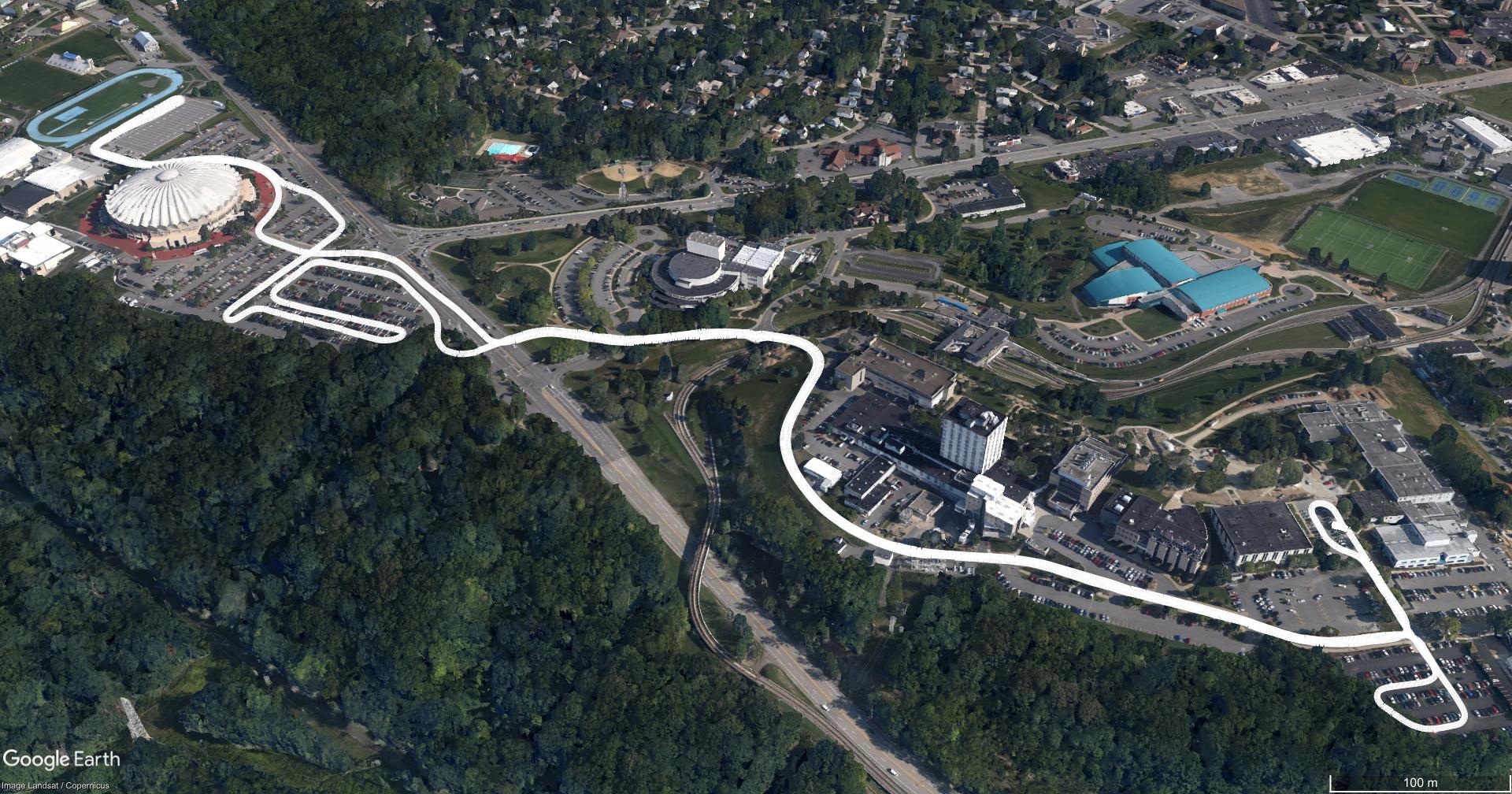
(a) Ground trace for first data collect.

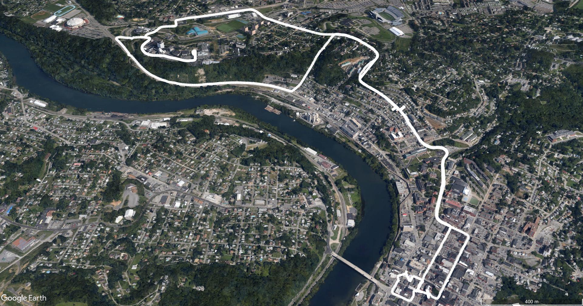
(b) Ground trace for second data collect.

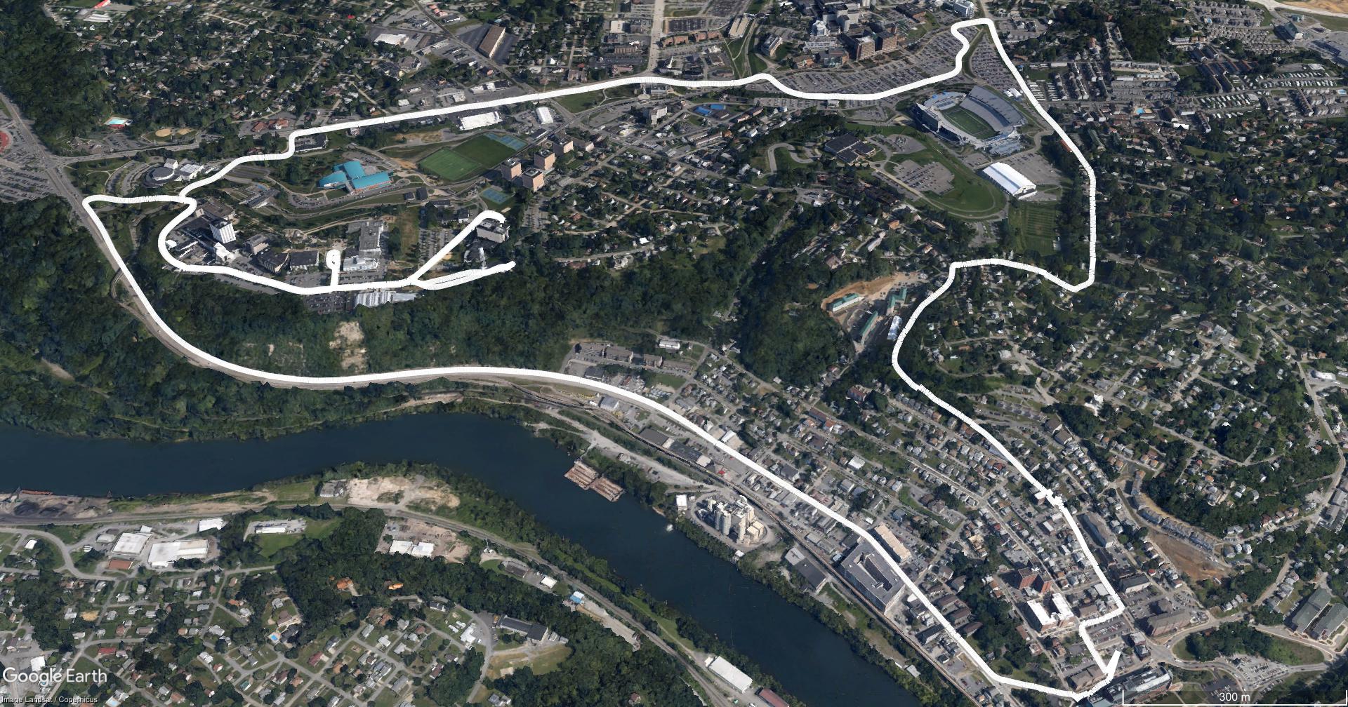
(c) Ground trace for third data collect.

Figure 5: Ground trace of three kinematic driving data sets collected in the Morgantown, WV area.

By altering the tracking parameters of the GPS SDR, it is possible to vary the accuracy of the GPS pseudorange and carrier-phase observables reported by the receiver. In particular, by changing the tracking loop noise bandwidths and the spacing of the early and late correlators, both the level of thermal noise errors [54] and the susceptibility to multipath errors can be varied [55]. As detailed in [54], the thermal noise of the Phase Lock Loop (PLL) is directly proportional to the square root of the selected noise loop bandwidth, $B_{\phi}$

$$\sigma_{PLL}=\frac{\lambda_{L1}}{2\pi}\sqrt{\frac{B_{\phi}}{C/N_{0}}\bigg{(}1+\frac{1}{2TC/N_{0}}\bigg{)}}$$ (28)

where $\lambda_{L1}$ is the GPS L1 wavelength, $B_{\phi}$ is the carrier loop bandwidth in units of Hz, $C/N_{0}$ is the carrier-to-noise ratio in Hz, and $T$ is the integration time.

Likewise, the code tracking jitter of the Delay Lock Loop (DLL) is dependent on both the selected noise bandwidth, $B_{\rho}$, and the spacing of the early and late correlators, $D_{EL}$, however, this error model is also dependent on the bandwidth of the radio frequency frond-end, $B_{fe}$, of the receiver and the chiprate of the signal being tracked. That is, if $D_{EL}$ is selected to be at or larger than $\pi$ multiplied by the ratio of the GPS C/A chipping rate, $R_{C/A}$, and $B_{fe}$, then the approximation of the code tracking noise jitter (in units of chips) is given as [54]

$$\sigma_{DLL}=\sqrt{\frac{B_{\rho}}{2C/N_{0}}D_{EL}\bigg{(}{1+\frac{2}{TC/N_{0}(2-D_{EL})}}\bigg{)}}$$ (29)

if $\big{(}\frac{R_{C/A}}{B_{fe}}<D_{EL}<\frac{\pi R_{C/A}}{B_{fe}}\big{)}$ , then the code tracking jitter is approximated as [54]

$$\sigma_{DLL}=\Bigg{[}\frac{B_{\rho}}{2C/N_{0}}\Bigg{(}\frac{1}{B_{fe}}+\frac{B_{fe}T_{c}}{\pi-1}\bigg{(}D_{EL}-\frac{1}{B_{fe}T_{c}}\bigg{)}^{2}\Bigg{)}$$

$$\times\Bigg{(}1+\frac{2}{TC/N_{0}(2-D_{EL})}\Bigg{)}\Bigg{]}^{1/2}.$$

Otherwise, if $\big{(}D_{EL}<\frac{R_{C/A}}{B_{fe}}\big{)}$, there is no additional benefit of further reducing $D_{EL}$, and the code noise error model reduces to a dependence on the front end and noise bandwidths[54].

$$\sigma_{DLL}=\sqrt{\frac{B_{\rho}}{2C/N_{0}}\bigg{(}\frac{1}{B_{fe}T_{c}}\bigg{)}\bigg{(}1+\frac{1}{TC/N_{0}}\bigg{)}}$$ (30)

For the experimental setup used in this study, the LabSat-3 has a $B_{fe}$ equal to 9.66 MHz and the GPS L1 C/A signal has a chiprate of 1.023 MHz, leading to a critical range of $D_{EL}\approx$ [0.11 .33]. An additional parameter that can be intuitively tuned in the GPS SDR configuration to provide an impact the observable quality is the rate at which the IQ data was sampled, $f_{s}$. In this setup, the LabSat-3 has a pre-defined sampling rate of 16.368 Mhz, but the data is down sampled to simulate reduced sampling quality in lower-cost receivers. Using these parameters, we are able to simulate a high-grade and low-grade quality GPS receiver using the parameters shown in Table III.

To quantify the accuracy of the generated observations, the zero-baseline test [56] was implemented. A zero-baseline test, as its name suggests, performs a doubled-differenced differential GPS baseline estimation between two sets of GPS receiver data that are known to have an a baseline of exactly zero. That is, in this set-up, the non-zero estimated baseline magnitude is known to be due to discrepancies in the GPS observables reported by the two different receivers. Using the high quality geodetic-grade GPS receiver observables as a reference, the zero-baseline tests provides a metric to assess the quality of the SDR receiver observables.

The zero-baseline test was implemented by first estimating the reference receiver solution and then configuring the RTKLIB DGPS software [57] to estimate a moving baseline double-differenced GPS solution between the observables reported by the reference receiver and the observables reported by the particular GPS SDR tracking configuration. Because the observables are generated from the same RF front end (i.e., the LabSat-3) and connected to the same antenna, the zero-baseline test results should provided zero difference, in an ideal scenario. The zero-baseline test results for the two resulting GPS SDR cases, which are utilized to experimentally validate the proposed approach within this paper, are shown in Table IV, where a large discrepancy can be see between the low-grade and high-grade observations.

TABLE III: GPS SDR observation tracking configurations utilized within this study.

GPS Quality	$f_{s}$ (MHz)	$D_{EL}$ (chips)	$B_{\rho}$ (Hz)	$B_{\phi}$ (Hz)
Low	4.092	0.5	2	50
High	16.368	0.2	1	25

TABLE IV: Zero-baseline observation comparison for kinematic data sets – see Fig. 5 – with varied GPS SDR tracking configurations, as specified in Table III.

Zero-Baseline Comparison Mean 3D Error (m.)	Collect 1	Collect 2	Collect 3
Low	16.20	37.44	29.43
High	0.59	18.03	17.48

The raw IQ recordings, GNSS-SDR processing configurations, and resulting observables in the Receiver Independent Exchange Format (RINEX) [58], that are used in this study have all been made publicly available at https://bit.ly/2vybpgA.

IV-B GPS Factor Graph Model

To utilize the collected GPS data within the factor graph framework, a likelihood factor must be constructed for the observations. To facilitate the construction of such a factor, the measurement model for the GPS L1-band pseudorange and carrier-phase observations will be discussed, as provided in Eq. 31 and Eq. 32, respectively. Within the pseudorange and carrier-phase observation models, the $X_{s}$ term is the known satellites location, $X_{u}$ is the estimated user location, and $||*||$ is the $l^{2}$-norm.

$$\begin{split}\rho^{i}_{L_{1}}=&\ ||X_{s}-X_{u}||+c(\delta t_{u}-\delta t_{s})+T_{z,d}\mathscr{M}_{d}(el^{j})\\ &+I_{L_{1}}+\delta_{Rel.}+\delta_{P.C.}+\delta_{D.C.B}+\epsilon^{j}_{\rho}\end{split}$$ (31)

$$\begin{split}\boldsymbol{\phi}^{i}_{L_{1}}=&\ ||X_{s}-X_{u}||+c(\delta t_{u}-\delta t_{s})+T_{z,d}\mathscr{M}_{d}(el^{j})\\ &-I_{L_{1}}+\delta_{Rel.}+\delta_{P.C.}+\delta_{W.U.}+\lambda_{IF}N^{j}_{IF}+\epsilon^{j}_{\phi}\end{split}$$ (32)

Contained within the models for the pseudorange and carrier-phase observations are several mutual terms, which can be decomposed into three categories. The first category is the propagation medium specific terms (i.e., the troposphere delay $T_{z,d}\mathscr{M}_{d}(el^{j})$ [59] and the ionospheric delay $I_{L1}$ [60]). The second category is the GPS receiver specific terms (i.e., the receiver clock bias $\delta t_{u}$, which must be incorporated into the state vector and estimated, and the observation uncertainty models $\epsilon$). The final category is the GPS satellite specific terms (i.e., the satellite receiver clock bias $\delta t_{s}$, the differential code bias correction $\delta_{D.C.B}$ [54], the relativistic satellite correction $\delta_{Rel.}$ [61], and the satellite phase center offset correction $\delta_{P.C}$ [62]).

Contained within the carrier-phase observation model (i.e., Eq. 32) are two terms that are not present in the pseudorange observation model. The first term is the carrier-phase windup [63], which can easily be modeled to mitigate its effect. The second term is the carrier-phase ambiguity [64], which can not be easily modeled, and thus, must be incorporated into the state vector and estimated.

Utilizing the provided observation model, the GPS factor graph constraint can be constructed. To begin, we assume that the GPS observation uncertainty model is a uni-modal Gaussian. With this assumption, the GPS observations can be incorporated into the factor graph formulation using the mahalanobis distance [65, 66], as provided in Eq. 33, where $y$ is the observed GPS measurement, $\hat{y}$ is the modeled observation (calculated using Eq. 31 or Eq. 32 for a pseudorange or carrier-phase observation, respectively), and $\Lambda$ is the measurement uncertainty model.

$$\psi(i)=\rvert\rvert y-\hat{y}\lvert\lvert_{\Lambda}$$ (33)

With the GPS observation factor, the desired states can be estimated using any NLLS algorithm [65], as discussed in section II. For this application, the state vector is defined in Eq. 34, where $\delta P$ is the 3-D user position state, $T_{z,w}$ is a state used to compensate for troposphere modeling errors, $\delta t_{u}$ is the receiver clock bias, and $N_{*}$ are the carrier-phase ambiguity terms for all observed satellites. For a thorough discussion on the resolution of carrier-phase ambiguity terms within the factor graph formulation, the reader is referred to [66].

$$X=\begin{pmatrix}\delta P\\ T_{z,w}\\ \delta t_{u}\\ N_{1}\\ \vdots\\ N_{n}\end{pmatrix}$$ (34)

To implement the provided model, this paper benefited from several open-source software packages. Specifically, to enable the implementation of the GPS observation modeling, the GPSTk software package [67] is utilized. For the factor graph construction and optimization, the Georgia Tech Smoothing and Mapping (GTSAM) library [68] is leveraged.

V Results

Utilizing the three kinematic data sets — as depicted in Fig. 5 — with varied receiver tracking metrics (i.e., the low quality and high quality receiver metrics, as discussed in Section IV), the proposed algorithm was tested with three state estimation techniques. The first algorithm used as a baseline comparison is a batch estimation strategy with an $l^{2}$-norm cost function. The second comparison algorithm is a batch estimator with the dynamic covariance scaling [14] robust kernel. This specific algorithm was selected because it is both a closed-form solution to the switch constraints technique [13], and a specific realization of the robust m-estimator. The final state estimation technique used to for this analysis is the max-mixtures [15] approach with a static measurement uncertainty model.

To generate the reference position solution which is utilized to enable a positioning error comparison, the GNSS observables reported by the reference GNSS receiver (i.e., a NovAtel OEM 638 Receiver) were used. Utilizing the baseline reference GPS measurements, the reference truth solution was generated through an iterative filter-smoother framework implemented within the open-source package RTKLIB [57].

V-A Positioning Performance Comparison

V-A1 Low Quality Observations

To begin an analysis, the discussed robust estimation techniques are evaluated when the algorithms are provided with low quality observations. As a metric to enable state estimation performance comparisons, the horizontal residual-sum-of-squares (RSOS) positioning error is utilized. Utilizing the horizontal RSOS positioning metric, a solution comparison is provided in the form of a box-plot, as depicted in Fig. 6. From Fig. 6, it can be seen that the proposed algorithm significantly reduces the median horizontal positioning error when compared to the reference robust estimation techniques on the three collect data sets – see Table V(c) for specific statistics. In addition to the median RSOS positioning error minimization, it is also noted that the proposed approach either outperforms or performs comparably to the three comparison approaches with respect to positioning solution variance and maximum error, as provided in Table V(c).

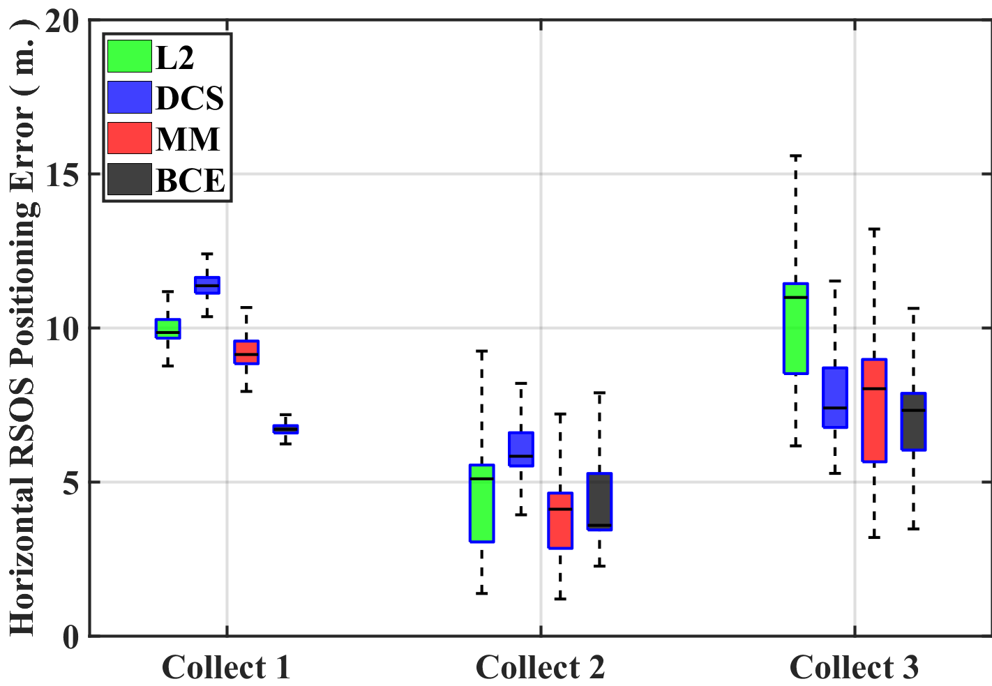
Figure 6: Box plot of RSOS positioning error for collected kinematic GNSS data sets with low quality – see Table III for GNSS receiver configuration – generated observations. The specific estimator statistics are provided in Table V(c). Within this figure, $L2$, is a batch estimator with $l^{2}$ cost function, DCS is the dynamic covariance scaling robust estimator, MM is the max-mixtures approach with a static measurement covariance model, and BCE is the proposed batch covariance estimation technique.

TABLE V: Horizontal RSOS positioning error results when low quality observations are utilized. The green and red cell entries correspond to the minimum and maximum statistic, respectively.

(a) Horizontal RSOS positioning error results for data collect 1 when low quality – see Table III for receiver configuration – observations are utilized.

(m.)	$L_{2}$	DCS	MM	BCE
median	9.84	10.82	9.13	6.70
variance	0.33	0.21	0.37	0.09
max	14.84	16.10	14.11	11.75

(b) Horizontal RSOS positioning error results for data collect 2 when low quality – see Table III for receiver configuration – observations are utilized.

(m.)	$L_{2}$	DCS	MM	BCE
median	5.09	5.02	4.11	3.58
variance	613.13	342.92	673.50	393.32
max	127.29	98.05	132.49	103.64

(c) Horizontal RSOS positioning error results for data collect 3 when low quality – see Table III for receiver configuration – observations are utilized.

(m.)	$L_{2}$	DCS	MM	BCE
median	10.98	9.88	8.02	7.31
variance	3.06	1.49	3.36	2.55
max	17.26	17.30	15.06	15.35

To depict the adaptive nature of the measurement uncertainty model within the proposed approach, the estimated pseudorange and carrier-phase uncertainty models (for data collect 1 with low-quality observation) as a function of optimization iteration are depicted in Figures 7, and 8, respectively. From Fig. 8 a large change in the structure of the assumed carrier-phase measurement uncertainty model can be seen. Specifically, the carrier-phase uncertainty model adapts from the assumed model (i.e, $y\sim\mathscr{N}(0,2.5\text{cm})$) to a highly multimodal GMM at the final iteration, as depicted in Fig. 8. As an additional visualization of the adaptive nature of the estimated covariance model, Fig. 9 is provided, which depicts the progression of the uncertainty model in the measurement residual domain for data collect 1 with low-quality observation as a function of the iteration of optimization.

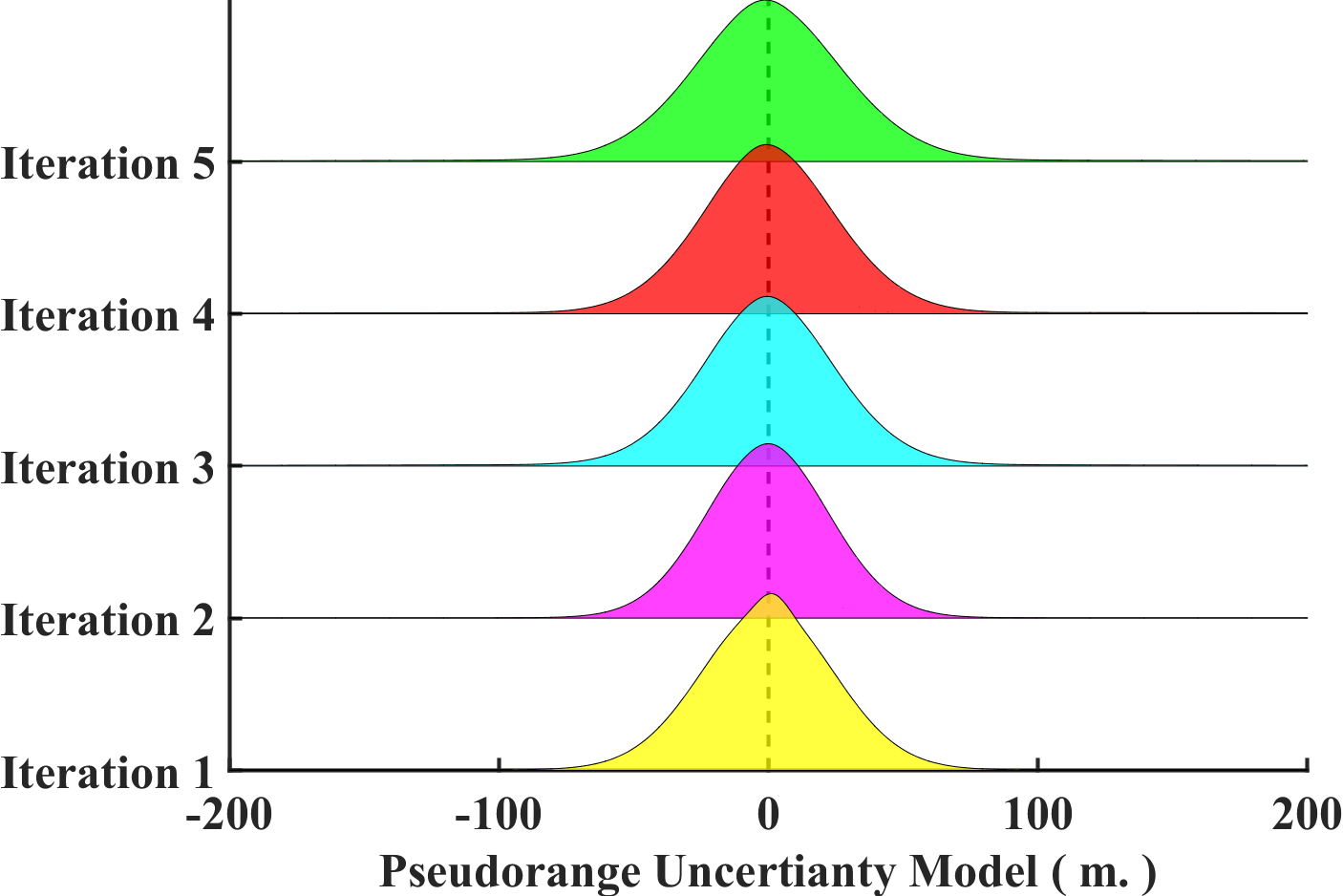
Figure 7: Evolution of the pseudorange Gaussian mixture model based uncertainty model for data collect 1 with low-quality observation as a function of optimizer iteration.

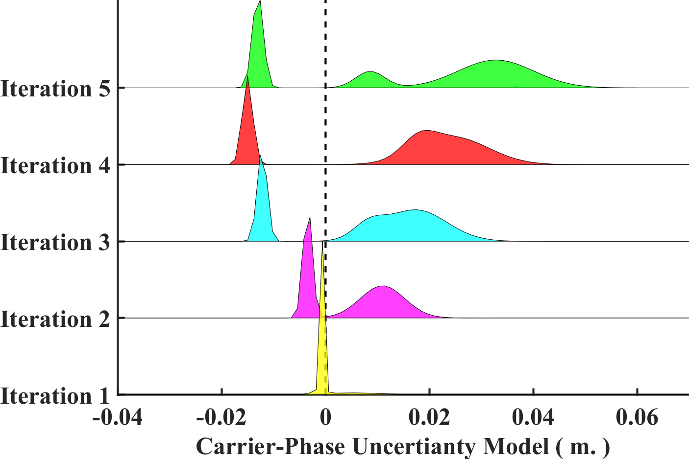
Figure 8: Evolution of the carrier-phase Gaussian mixture model based uncertainty model for data collect 1 with low-quality observation as a function of optimizer iteration.

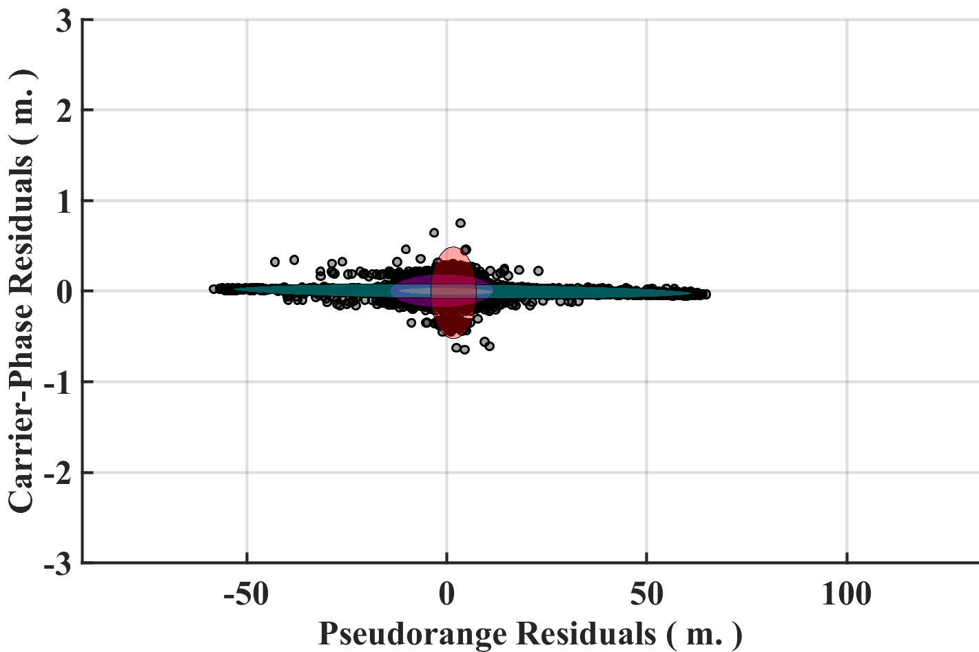
(a) First Iteration

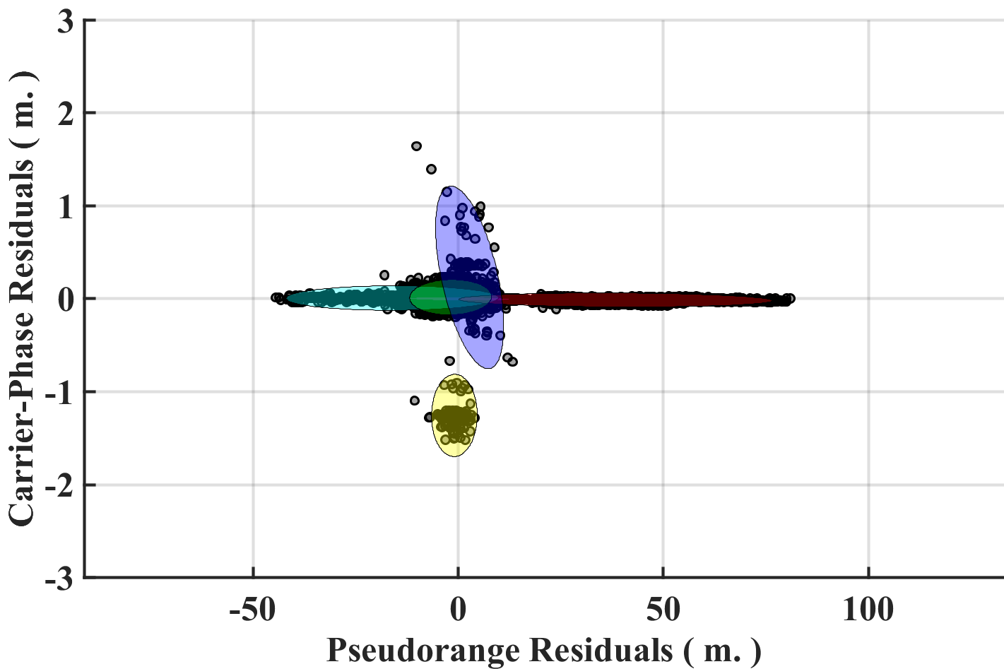
(b) Third Iteration

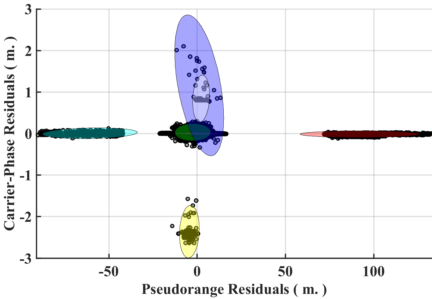
(c) Fifth (Final) Iteration

Figure 9: Progression of GNSS observation residuals with multimodal measurement error covariance – as estimated by the proposed approach which utilizes variational inference to generate a Gaussian mixture model uncertainty representation from the estimators residuals – for data collect 1 with low-quality observations.

V-A2 High Quality Observations

The high quality observations were also evaluated with the same four state estimation techniques. The horizontal RSOS positioning errors are depicted in box plot format in Figure 10. From Fig. 10 it is shown that all four estimators provide similar horizontal positioning accuracy – see Table VI(c) for complete statistics.

The comparable horizontal RSOS positioning performance of all four estimation on the provided high quality observations is to be expected. This comparability, when provided with high quality observations, is because the a priori assumed model closely resembles the observed model. This means that no benefit is granted by having a robust or adaptive state estimation framework in place.

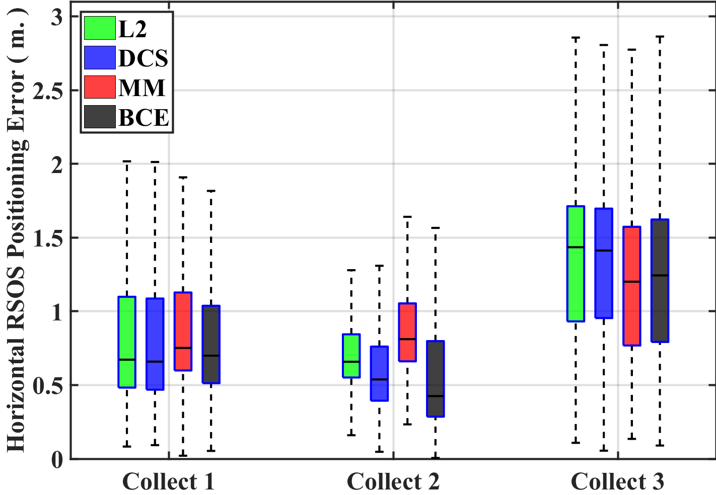
Figure 10: Box plot of RSOS positioning error for collected kinematic GNSS data sets with high quality – see Table III for GNSS receiver configuration – generated observations. The specific estimator statistics are provided in Table VI(c). Within this figure, $L2$, is a batch estimator with $l^{2}$ cost function, DCS is the dynamic covariance scaling robust estimator, MM is the max-mixtures approach with a static measurement covariance model, and BCE is the proposed batch covariance estimation technique.

TABLE VI: Horizontal RSOS positioning error results when high quality observations are utilized. The green and red cell entries correspond to the minimum and maximum statistic, respectively.

(a) Horizontal RSOS positioning error results for data collect 1 when high quality – see Table III for receiver configuration – observations are utilized.

(m.)	$L_{2}$	DCS	MM	BCE
median	0.68	0.67	0.75	0.69
variance	0.17	0.17	0.17	0.15
max	6.30	6.30	6.37	6.34

(b) Horizontal RSOS positioning error results for data collect 2 when high quality – see Table III for receiver configuration – observations are utilized.

(m.)	$L_{2}$	DCS	MM	BCE
median	0.65	0.65	0.81	0.42
variance	11.27	11.27	11.94	16.60
max	18.29	18.30	18.91	21.73

(c) Horizontal RSOS positioning error results for data collect 3 when high quality – see Table III for receiver configuration – observations are utilized.

(m.)	$L_{2}$	DCS	MM	BCE
median	1.44	1.43	1.20	1.24
variance	0.30	0.30	0.30	0.26
max	9.52	17.30	9.43	9.44

To verify that the assumed measurement model closely resembles the observed model, the estimated covariance of the proposed approach can be examined for a specific data set (i.e., data collect 1, as depicted in Fig. 11). For data collect 1 with high quality observations, the measurement uncertainty model estimated by the proposed approach has two modes, as depicted in Fig. 11. One of the modes — specifically, the mode that characterizes approximately 90% of the measurements — closely resembles the assumed a priori measurement uncertainty model. For comparison, the specific values of the a priori measurement uncertainty model ($\Lambda$), and the estimated measurement uncertainty model ($\hat{\Lambda}$) as provided by the proposed approach, are provided below.

$$\Lambda=\left[{\begin{array}[]{*{20}c}2.5^{2}&0.0\\ 0.0&0.025^{2}\\ \end{array}}\right]\quad\quad\hat{\Lambda}=\left[{\begin{array}[]{*{20}c}1.7^{2}&0.0\\ 0.0&0.0017^{2}\\ \end{array}}\right]$$

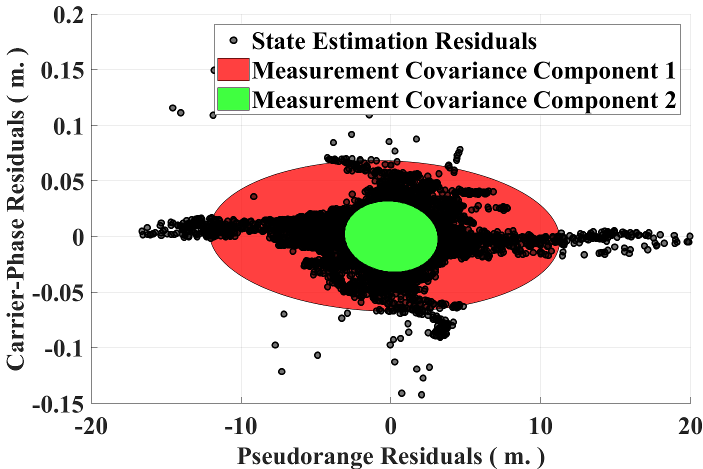
Figure 11: Measurement residuals with associated BCE estimated measurement error covariance – each ellipse represents 95% confidence – for data collect 1 with high quality observations.

V-B A Priori Information Sensitivity Comparison

To continue the analysis, an evaluation of each estimation framework’s sensitivity to the a priori information is provided. Specifically, it is of interest to evaluate the sensitivity of the estimation frameworks to the a priori measurement error covariance model.

To enable this estimator sensitivity evaluation, the low-quality observations generated from data collect 1 are utilized. With these generated observations, the estimation framework’s sensitivity is quantified by evaluating the response – which is quantified by the horizontal RSOS positioning error – of each estimator as a function of the a priori covariance model. For this study, the a priori covariance model will be a scaled version of the assumed measurement error covariance model, as depicted below.

$$\Lambda=s\cdot\left[{\begin{array}[]{*{20}c}2.5^{2}&0.0\\ 0.0&0.025^{2}\\ \end{array}}\right]$$

This sensitivity evaluation is presented graphically within Fig. 12. From this figure, it is shown that all the estimation frameworks show at least a slight sensitivity to the a priori measurement error covariance model; however, some estimation frameworks are significantly more sensitive to perturbation in the a priori covariance model than other (e.g., the L2 and DCS estimators showing the greatest sensitivity). From this figure, it is also shown that the proposed BCE approach is significantly less sensitivity to perturbations of the a priori measurement error covariance model when compared to the other estimators.

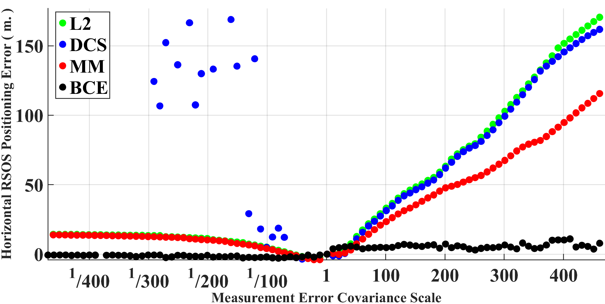
Figure 12: Sensitivity of the estimation frameworks to the selection of an a priori measurement error covariance model. Within this figure, $L2$ is a batch estimator with $l^{2}$ cost function, DCS is the dynamic covariance scaling robust estimator, MM is the max-mixtures approach with a static measurement covariance model, and BCE is the proposed batch covariance estimation technique.

V-C Run-time Comparison

To conclude the evaluation of the proposed estimation framework, a run-time comparison is provided. To quantify a run-time evaluation, the wall-clock time (i.e., the total execution time of the utilized estimation framework) divided by the cardinality of the utilized data collect is employed as the metric of comparison. This metric is selected because it enables a run-time comparison regardless of the data collect (i.e., each data collect has a different number of observations so, dividing by the cardinality enables a fair run-time comparison across sets). To implement the run-time comparison, a quad-core Intel i5-6400 central processing unit (CPU) that has a base processing frequency of 2.7 GHz was utilized.

Utilizing the specified hardware and evaluation metric, the run-time comparison is presented within Fig. 13 for the four estimation algorithms. From Fig. 13, it is shown that the traditional $l^{2}$ approach provides the fastest run-time, with the max-mixtures approach providing comparable results. Additionally, it is shown that the batch covariance estimation approach is the most computationally expensive approach.

The increased computational complexity of the proposed approach is primarily due to the GMM fitting procedure. To reduce the computation requirement of the proposed estimation framework, several research directions could be explored. For example, rather than utilizing all calculated residuals to characterize the measurement uncertainty model, a sub-sampling based approach per iteration could be utilized [69]. This modification has the potential to significantly decease the run-time of the employed variational clustering algorithm which, in turn, would decrease the run-time of the associated BCE approach.

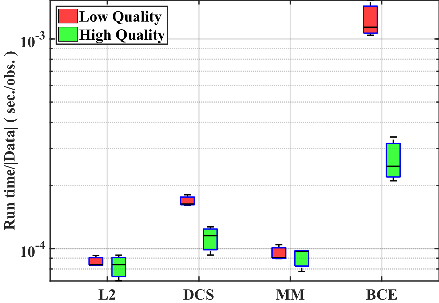
Figure 13: Wall-clock time per utilized observation for each of the estimation frameworks, where $L2$ is a batch estimator with $l^{2}$ cost function, DCS is the dynamic covariance scaling robust estimator, MM is the max-mixtures approach with a static measurement covariance model, and BCE is the proposed batch covariance estimation technique.

VI Conclusion

Several robust state estimation frameworks have been proposed over the previous decades. Underpinning all of these robust frameworks is one dubious assumption. Specifically, the assumption that an accurate a priori measurement uncertainty model can be provided. As systems become more autonomous, this assumption becomes less valid (i.e., as systems start operating in novel environments, there is no guarantee that the assumed a priori measurement uncertainty model characterizes the sensors current observation uncertainty).

In an attempt to relax this assumption, a novel robust state estimation framework is proposed. The proposed framework enables robust state estimation through the iterative adaptation of the measurement uncertainty model. The adaptation of the measurement uncertainty model is granted through non-parametric clustering of the estimators residuals, which enables the characterization of the measurement uncertainty via a Gaussian mixture model. This Gaussian mixture model based measurement uncertainty characterization can be incorporated into any non-linear least square optimization routine by only using the single assigned — the assignment of each observation to a single mode within the mixture model is provided by the utilized non-parametric clustering algorithm — component’s sufficient statistics from within the mixture model to update the uncertainty model for all observation (i.e., every observations uncertainty model is approximately characterized by the single assigned Gaussian component from within the mixture model).

To verify the proposed algorithm, several GNSS data sets were collected. The collected data sets provide varying levels of observation degradation to enable to characterization of the proposed algorithm on a diverse data set. Utilizing these data sets, it is shown that the proposed technique exhibits improved state estimation accuracy when compared to other robust estimation techniques when confronted with degraded data quality.

References

- [1] R. R. Murphy, Disaster robotics. MIT press, 2014.
- [2] D. Wettergreen, G. Foil, M. Furlong, and D. R. Thompson, “Science autonomy for rover subsurface exploration of the atacama desert,” AI Magazine, vol. 35, no. 4, pp. 47–60, 2014.
- [3] L. D. Riek, “Healthcare robotics,” arXiv preprint arXiv:1704.03931, 2017.
- [4] D. Simon, Optimal state estimation: Kalman, H infinity, and nonlinear approaches. John Wiley & Sons, 2006.
- [5] E. De Klerk, C. Roos, and T. Terlaky, “Nonlinear optimization (co 367),” 2004.
- [6] Y.-x. Yuan, “A review of trust region algorithms for optimization,” in Iciam, vol. 99, 2000, pp. 271–282.
- [7] R. E. Kalman, “A new approach to linear filtering and prediction problems,” Journal of basic Engineering, vol. 82, no. 1, pp. 35–45, 1960.
- [8] D. P. Bertsekas, “Incremental least squares methods and the extended Kalman filter,” SIAM Journal on Optimization, vol. 6, no. 3, pp. 807–822, 1996.
- [9] S. J. Julier and J. K. Uhlmann, “New extension of the Kalman filter to nonlinear systems,” in Signal processing, sensor fusion, and target recognition VI, vol. 3068. International Society for Optics and Photonics, 1997, pp. 182–194.
- [10] M. C. Graham, “Robust bayesian state estimation and mapping,” Ph.D. dissertation, Massachusetts Institute of Technology, 2015.
- [11] F. R. Hampel, “Contribution to the theory of robust estimation,” Ph. D. Thesis, University of California, Berkeley, 1968.
- [12] P. J. Huber, Robust Statistics. Wiley New York, 1981.
- [13] N. Sünderhauf, “Robust optimization for simultaneous localization and mapping,” Ph.D. dissertation, Technischen Universitat Chemnitz, 2012.
- [14] P. Agarwal, G. D. Tipaldi, L. Spinello, C. Stachniss, and W. Burgard, “Robust map optimization using dynamic covariance scaling,” in 2013 IEEE International Conference on Robotics and Automation. Citeseer, 2013, pp. 62–69.
- [15] E. Olson and P. Agarwal, “Inference on networks of mixtures for robust robot mapping,” The International Journal of Robotics Research, vol. 32, no. 7, pp. 826–840, 2013.
- [16] M. A. Fischler and R. C. Bolles, “Random sample consensus: a paradigm for model fitting with applications to image analysis and automated cartography,” Communications of the ACM, vol. 24, no. 6, pp. 381–395, 1981.
- [17] Y. Latif, C. Cadena, and J. Neira, “Realizing, reversing, recovering: Incremental robust loop closing over time using the irrr algorithm,” in 2012 IEEE/RSJ International Conference on Intelligent Robots and Systems. IEEE, 2012, pp. 4211–4217.
- [18] L. Carlone, A. Censi, and F. Dellaert, “Selecting good measurements via relaxation: A convex approach for robust estimation over graphs,” in 2014 IEEE/RSJ International Conference on Intelligent Robots and Systems. IEEE, 2014, pp. 2667–2674.
- [19] Y. Zhai, M. Joerger, and B. Pervan, “Fault exclusion in multi-constellation global navigation satellite systems,” The Journal of Navigation, vol. 71, no. 6, pp. 1281–1298, 2018.
- [20] R. M. Watson, C. N. Taylor, R. C. Leishman, and J. N. Gross, “Batch Measurement Error Covariance Estimation for Robust Localization,” in ION GNSS+ 2018. the Institute of Navigation, 2018, pp. 2429–2439.
- [21] T. Pfeifer and P. Protzel, “Expectation-maximization for adaptive mixture models in graph optimization,” arXiv preprint arXiv:1811.04748, 2018.
- [22] K. Kurihara, M. Welling, and N. Vlassis, “Accelerated variational Dirichlet process mixtures,” in Advances in neural information processing systems, 2007, pp. 761–768.
- [23] D. Steinberg, “An unsupervised approach to modelling visual data,” Ph.D. dissertation, University of Sydney., 2013.
- [24] J. S. Liu, “The collapsed Gibbs sampler in Bayesian computations with applications to a gene regulation problem,” Journal of the American Statistical Association, vol. 89, no. 427, pp. 958–966, 1994.
- [25] F. R. Kschischang, B. J. Frey, and H.-A. Loeliger, “Factor graphs and the sum-product algorithm,” IEEE Transactions on information theory, vol. 47, no. 2, pp. 498–519, 2001.
- [26] F. Dellaert, M. Kaess et al., “Factor graphs for robot perception,” Foundations and Trends® in Robotics, vol. 6, no. 1-2, pp. 1–139, 2017.
- [27] K. Madsen, H. B. Nielsen, and O. Tingleff, “Methods for Non-Linear Least Squares Problems (2nd ed.),” Informatics and Mathematical Modelling, Technical University of Denmark, DTU, p. 60, 2004.
- [28] J. J. Moré, “The Levenberg-Marquardt algorithm: implementation and theory,” in Numerical analysis. Springer, 1978, pp. 105–116.
- [29] M. J. Powell, “A new algorithm for unconstrained optimization,” Nonlinear programming, pp. 31–65, 1970.
- [30] P. J. Huber et al., “Robust estimation of a location parameter,” The Annals of Mathematical Statistics, vol. 35, no. 1, pp. 73–101, 1964.
- [31] K. MacTavish and T. D. Barfoot, “At all costs: A comparison of robust cost functions for camera correspondence outliers,” in 2015 12th Conference on Computer and Robot Vision. IEEE, 2015, pp. 62–69.
- [32] P. W. Holland and R. E. Welsch, “Robust regression using iteratively reweighted least-squares,” Communications in Statistics-theory and Methods, vol. 6, no. 9, pp. 813–827, 1977.
- [33] M. Bosse, G. Agamennoni, I. Gilitschenski et al., “Robust estimation and applications in robotics,” Foundations and Trends® in Robotics, vol. 4, no. 4, pp. 225–269, 2016.
- [34] Z. Zhang, “Parameter estimation techniques: A tutorial with application to conic fitting,” Image and vision Computing, vol. 15, no. 1, pp. 59–76, 1997.
- [35] T. D. Barfoot, State Estimation for Robotics. Cambridge University Press, 2017.
- [36] N. Sünderhauf and P. Protzel, “Switchable constraints for robust pose graph SLAM,” in 2012 IEEE/RSJ International Conference on Intelligent Robots and Systems. IEEE, 2012, pp. 1879–1884.
- [37] C. Zach and G. Bourmaud, “Iterated lifting for robust cost optimization,” in BMVC, 2017.
- [38] P. Agarwal, “Robust graph-based localization and mapping,” Ph.D. dissertation, University of Freiburg, Germany, 2015.
- [39] C. M. Bishop, Pattern recognition and machine learning. Springer, 2006.
- [40] F. Dellaert and M. Kaess, “Square Root SAM: Simultaneous Localization and Mapping via Square Root Information Smoothing,” The International Journal of Robotics Research, vol. 25, no. 12, pp. 1181–1203, 2006.
- [41] B. A. Frigyik, A. Kapila, and M. R. Gupta, “Introduction to the Dirichlet distribution and related processes,” Department of Electrical Engineering, University of Washignton, UWEETR-2010-0006, no. 0006, pp. 1–27, 2010.
- [42] P. Diaconis and D. Ylvisaker, “Conjugate priors for exponential families,” The Annals of statistics, pp. 269–281, 1979.
- [43] S. Tu, “The Dirichlet-multinomial and Dirichlet-categorical models for Bayesian inference,” Computer Science Division, UC Berkeley, 2014.
- [44] K. P. Murphy, “Conjugate Bayesian analysis of the Gaussian distribution,” def, vol. 1, no. 22, p. 16, 2007.
- [45] I. Alvarez, J. Niemi, and M. Simpson, “Bayesian inference for a covariance matrix,” arXiv preprint arXiv:1408.4050, 2014.
- [46] M. I. Jordan et al., “Graphical models,” Statistical Science, vol. 19, no. 1, pp. 140–155, 2004.
- [47] M. Beal, “Variational algorithms for approximate bayesian inference,” Ph.D. dissertation, University of London, 2003.
- [48] A. Doucet and X. Wang, “Monte carlo methods for signal processing: a review in the statistical signal processing context,” IEEE Signal Processing Magazine, vol. 22, no. 6, pp. 152–170, 2005.
- [49] D. M. Blei, A. Kucukelbir, and J. D. McAuliffe, “Variational inference: A review for statisticians,” Journal of the American Statistical Association, vol. 112, no. 518, pp. 859–877, 2017.
- [50] J. Liao and A. Berg, “Sharpening jensen’s inequality,” The American Statistician, pp. 1–4, 2018.
- [51] R. Harpaz and R. Haralick, “The EM algorithm as a lower bound optimization technique,” CUNY Ph. D. Program in Computer Science Technical Reports, pp. 1–14, 2006.
- [52] “LabSat 3 GPS Simulator,” https://www.labsat.co.uk/index.php/en/products/labsat-3, accessed 3/1/19.
- [53] C. Fernandez-Prades, J. Arribas, P. Closas, C. Aviles, and L. Esteve, “GNSS-SDR: an open source tool for researchers and developers,” in Proceedings of the 24th International Technical Meeting of The Satellite Division of the Institute of Navigation (ION GNSS 2011), 2001, pp. 780–0.
- [54] E. Kaplan and C. Hegarty, Understanding GPS: principles and applications. Artech house, 2005.
- [55] A. Van Dierendonck, P. Fenton, and T. Ford, “Theory and performance of narrow correlator spacing in a GPS receiver,” Navigation, vol. 39, no. 3, pp. 265–283, 1992.
- [56] P. Misra and P. Enge, “Global Positioning System: signals, measurements and performance second edition,” Massachusetts: Ganga-Jamuna Press, 2006.
- [57] T. Takasu, “RTKLIB: An open source program package for GNSS positioning,” 2011.
- [58] W. Gurtner and L. Estey, “Rinex-the receiver independent exchange format-version 3.00,” Astronomical Institute, University of Bern and UNAVCO, Bolulder, Colorado., 2007.
- [59] A. Niell, “Global mapping functions for the atmosphere delay at radio wavelengths,” Journal of Geophysical Research: Solid Earth, vol. 101, no. B2, pp. 3227–3246, 1996.
- [60] J. A. Klobuchar, “Ionospheric time-delay algorithm for single-frequency GPS users,” IEEE Transactions on aerospace and electronic systems, no. 3, pp. 325–331, 1987.
- [61] J.-F. Pascual-Sánchez, “Introducing relativity in global navigation satellite systems,” Annalen der Physik, vol. 16, no. 4, pp. 258–273, 2007.
- [62] P. Heroux, J. Kouba, P. Collins, and F. Lahaye, “GPS carrier-phase point positioning with precise orbit products,” in Proceedings of the KIS, 2001, pp. 5–8.
- [63] J.-T. Wu, S. C. Wu, G. A. Hajj, W. I. Bertiger, and S. M. Lichten, “Effects of antenna orientation on GPS carrier phase,” in Astrodynamics 1991, 1992, pp. 1647–1660.
- [64] D. Laurichesse, F. Mercier, J.-P. BERTHIAS, P. Broca, and L. Cerri, “Integer ambiguity resolution on undifferenced GPS phase measurements and its application to ppp and satellite precise orbit determination,” Navigation, vol. 56, no. 2, pp. 135–149, 2009.
- [65] N. Sünderhauf, M. Obst, G. Wanielik, and P. Protzel, “Multipath mitigation in GNSS-based localization using robust optimization,” in 2012 IEEE Intelligent Vehicles Symposium. IEEE, 2012, pp. 784–789.
- [66] R. M. Watson and J. N. Gross, “Evaluation of kinematic precise point positioning convergence with an incremental graph optimizer,” in 2018 IEEE/ION Position, Location and Navigation Symposium (PLANS). IEEE, 2018, pp. 589–596.
- [67] R. B. Harris and R. G. Mach, “The GPSTk: an open source GPS toolkit,” GPS Solutions, vol. 11, no. 2, pp. 145–150, 2007.
- [68] F. Dellaert, “Factor graphs and GTSAM: A hands-on introduction,” Georgia Institute of Technology, Tech. Rep., 2012.
- [69] D. M. Rocke and J. Dai, “Sampling and Subsampling for Cluster Analysis in Data Mining: With Applications to Sky Survey Data,” Data Mining and Knowledge Discovery, vol. 7, no. 2, pp. 215–232, 2003.