Joint Semantic Domain Alignment and
Target Classifier Learning for
Unsupervised Domain Adaptation

Abstract

Unsupervised domain adaptation aims to transfer the classifier learned from the source domain to the target domain in an unsupervised manner. With the help of target pseudo-labels, aligning class-level distributions and learning the classifier in the target domain are two widely used objectives. Existing methods often separately optimize these two individual objectives, which makes them suffer from the neglect of the other. However, optimizing these two aspects together is not trivial. To alleviate the above issues, we propose a novel method that jointly optimizes semantic domain alignment and target classifier learning in a holistic way. The joint optimization mechanism can not only eliminate their weaknesses but also complement their strengths. The theoretical analysis also verifies the favor of the joint optimization mechanism. Extensive experiments on benchmark datasets show that the proposed method yields the best performance in comparison with the state-of-the-art unsupervised domain adaptation methods.

1 Introduction

Deep Neural Networks (DNNs) have achieved a great success on many tasks such as image classification when a large set of labeled examples are available [1, 2, 3, 4]. However, in many real-world applications, there are plentiful unlabeled data but very limited labeled data; and the acquisition of labels is costly, or even infeasible. Unsupervised domain adaptation is a popular way to address this issue. It aims at transferring a well-performing model learned from a source domain to a different but related target domain when the labeled data from the target domain is not available [5].

Most efforts on unsupervised domain adaptation devote to reducing the domain discrepancy, such that a well-trained classifier in the source domain can be applied to the target domain [6, 7, 8, 9, 10]. However, these methods only align the distributions in the domain-level, and fail to consider the class-level relations among the source and target samples. For example, a car in the target domain may be mistakenly aligned to a bike in the source domain. To alleviate the class-level misalignment, semantic domain alignment methods [11, 12, 13, 14, 15] that enforce the samples from the same class to be close across domains are proposed. However, these domain alignment methods neglect the structures in target domain itself. Target classifier learning methods [16, 17] learn target discriminative features by distinguishing the samples in the target domain directly. Nonetheless, they may miss some important supervised information in the source domain. Intuitively, a straightforward method is to optimize semantic domain alignment and target classifier learning jointly. The joint optimization mechanism can not only eliminate their weaknesses, but also complement their strengths. The semantic domain alignment methods enforce the intra-class compactness, distinguishing different samples from the target domain. The target classifier learning methods enforce the inter-class discrepancy in the target domain, which in turn help to align the same class samples between two domains. However, as shown in Figure 1 (a) and (b), semantic domain alignment works in the feature space while target classifier learning works in the label space. Thus, optimizing them together is not a trivial task.

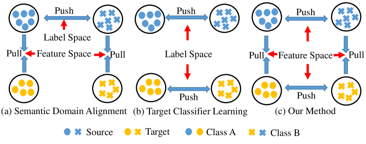
Figure 1: Comparisons of semantic domain alignment methods, target classifier learning methods and our proposed method. Note that we jointly optimize semantic domain alignment and target classifier learning in the feature space.

In this paper, we propose a novel unsupervised domain adaption method that jointly optimizes semantic domain alignment and target classifier learning in a holistic way. The proposed method is called SDA-TCL, which is short for Semantic Domain Alignment and Target Classifier Learning. Figure 1 (c) illustrats its basic idea. We utilize class centers in the feature space as the bridge to jointly optimize semantic domain-invariant features and target discriminative features both in the feature space. For target classifier learning, we design the discriminative center loss to learn discriminative features directly by pulling the samples toward their corresponding centers according to their pseudo-labels and pushing them away from the other centers. For semantic domain alignment, we share the class centers between the same classes across domains to pull the samples from the same class together. The main contributions of this paper are as follows:

• To the best of our knowledge, this is the first work trying to understand the relationship between semantic domain alignment and target classifier learning.

• We propose a novel method called Semantic Domain Alignment and Target Classifier Learning (SDA-TCL), which can jointly optimize semantic domain alignment and target classifier learning in a holistic way.

• We show both theoretically and empirically that the proposed joint optimization mechanism is highly effective.

2 Related Work

In this paper, we focus on the problem of deep unsupervised domain adaptation for image classification, and many works along this line of research have been proposed  [18, 19, 10, 16, 20].

These works can be roughly divided into the following two categories: The first one is to align distributions between the source and the target domain. Its main idea is to reduce the discrepancy between two domains such that a classifier learned from the source domain may be directly applied to the target domain. Under this motivation, multiple methods have been used to align the distributions of two domains, such as maximum mean discrepancy (MMD) [6, 7, 18], CORrelation ALignment (CORAL) [8, 21], attention [22], and optimal transport [23]. Besides, adversarial learning is also used to learn domain-invariant features [9, 10, 24, 20]. On par with these methods aligning distributions in the feature space, some methods align distributions in raw pixel space by translating source data to the target domain with Image to Image translation techniques [25, 26, 27, 28, 29, 30]. In addition to domain-level distribution alignment, the class-level information in target data is also frequently used to align class-level distributions [11, 12, 14, 13, 15, 31]. Compared with these methods, our method not only aligns class-level distributions, but also learns target discriminative features.

The second one is to capture target-specific structures by constructing a reconstruction network [32, 33], adjusting the distances between target samples and decision boundaries [34, 35, 36], seeking for density-based separations or clusters [37, 38, 39, 40, 41, 42] and learning target classifiers directly [16, 17]. Compared with these methods, our method not only learns target classifiers but also aligns class-level distributions, thus is more desirable.

3 Methodology

In unsupervised domain adaptation, we have a labeled source data set $\mathcal{D}^{s}=\{(x_{i}^{s},y_{i}^{s})|i=1,2,\ldots,N^{s}\}$ and a unlabeled target data set $\mathcal{D}^{t}=\{(x_{i}^{t})|i=1,2,\ldots,N^{t}\}$. Suppose the source data have $C$ classes, which is shared with the target data. Our goal is to learn a model from the data set $\mathcal{D}^{s}\cup\mathcal{D}^{t}$ to classify the samples in $\mathcal{D}^{t}$. Assume that each class in source (target) data has its corresponding source (target) class center $c_{j}^{s}$ ($c_{j}^{t}$) ($j\in\mathcal{C}=\{1,2,\ldots,C\}$) to represent it in the feature space. In our method, the target sample $x_{i}^{t}$ is classified according to its closest target center in the feature space. A generator network $G$ (parametrized by $\theta_{G}$) is utilized to generate the features, denoted by $G(x_{i}^{s})$ for the source sample $x_{i}^{s}$ and $G(x_{i}^{t})$ for the target sample $x_{i}^{t}$.

We aim to jointly optimize semantic domain-invariant features and target discriminative features in the feature space. As illustrated in Figure 2, our loss function consists of three parts: 1) $L_{s}(\theta_{G})$: It learns discriminative features for source domain by pulling the source sample toward its corresponding source center according to its label and pushing it away from the other source centers. 2) $L_{t}(\theta_{G})$: It learns discriminative features for target domain by pulling the target sample toward its corresponding target center according to its pseudo-label and pushing it away from the other target centers. 3) $L_{c}(\theta_{G})$ : It aligns class-level distributions by pulling the source center and the target center from the same class. We jointly optimize them:

$$L_{G}(\theta_{G})=L_{s}(\theta_{G})+\lambda_{t}L_{t}(\theta_{G})+\lambda_{c}L_{c}(\theta_{G})+\lambda_{d}L_{d}(\theta_{G}),$$ (1)

where $\lambda_{d}$, $\lambda_{t}$ and $\lambda_{c}$ are the balance parameters and $L_{d}(\theta_{G})$ is used to align domain-level distributions for providing a initial classifier to label the pseudo-labels following the previous methods [11, 14].

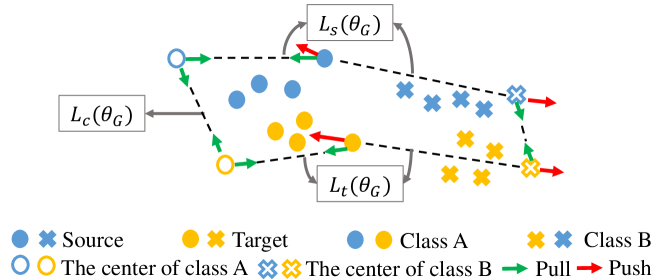
Figure 2: Illustration our proposed method SDA-TCL. We jointly optimize semantic domain alignment and target classifier learning in the feature space by optimizing $L_{s}(\theta_{G})$, $L_{t}(\theta_{G})$ and $L_{c}(\theta_{G})$.

3.1 Learning Source Discriminative Features

We aim to pull the source sample toward its corresponding source center and push it away from the other source centers. Here, we design discriminative center loss, which requires that the distances between samples and centers from the same class are smaller than a margin $\alpha$ and the distances between samples and centers from different classes are larger than a margin $\beta$. The discriminative center loss be formulated as:

$$L_{s}(\theta_{G})=\sum_{i=1}^{N^{s}}\Big{(}[d(G(x_{i}^{s}),c_{y_{i}^{s}}^{s})-\alpha]_{+}+[\beta-d(G(x_{i}^{s}),c_{\widetilde{y}_{i}^{s}}^{s})]_{+}\Big{)},$$ (2)

where $d(G(x_{i}^{s}),c_{j}^{s})$ denotes the squared Euclidean distance between sample $x_{i}^{s}$ and center $c_{j}^{s}$, and

$$\widetilde{y}_{i}^{s}=\mathop{\arg\min}\limits_{j\in\mathcal{C},j\neq y_{i}^{s}}d(G(x_{i}^{s}),c_{j}^{s})$$ (3)

denotes the closest negative center for sample $x_{i}^{s}$ in source centers, and $[a]_{+}$ denotes the rectifier function which is equal to $\max(0,a)$.

Note that we do not utilize softmax loss for classification but design the discriminative center loss. The discriminative center loss has two advantages compared with softmax loss: 1) The discriminative center loss enforces the intra-class compactness, which is helpful to pull ambiguous features away from the class boundaries [34, 35]; and 2) The discriminative center loss distinguishes the samples in the feature space directly, which makes it work in the same space with the class-level alignment.

3.2 Learning Target Discriminative Features

For the target domain, we aim to learn discriminative features directly in the feature space like source domain. Here, we optimize $L_{t}(\theta_{G})$ by utilizing the designed discriminative center loss to pull the target sample toward its corresponding target center according to its pseudo-label and push it away from the other target centers, which can be formulated as:

$$\small L_{t}(\theta_{G})=\sum_{i=1}^{N^{t}}w_{i}\Big{(}[{d(G(x_{i}^{t}),c_{\hat{y}_{i}^{t}}^{t})}-\alpha]_{+}+[\beta-d(G(x_{i}^{t}),c_{\widetilde{y}_{i}^{t}}^{t})]_{+}\Big{)},$$ (4)

where $\hat{y}_{i}^{t}$ denotes the pseudo-label for sample $x_{i}^{t}$, $\widetilde{y}_{i}^{t}$ denotes the closest negative target center for sample $x_{i}^{t}$ and $w_{i}$ is the sample weight

$$w_{i}=\frac{d(G(x_{i}^{t}),c_{\widetilde{y}_{i}^{t}})}{d(G(x_{i}^{t}),c_{\hat{y}_{i}^{t}})}-1.$$ (5)

Then we scale $w_{i}$ to [0, 1] within the same class. A target sample closer to its center than other centers will get a big $w_{i}$, which means the center is more confident on this sample. Target pseudo-labels are widely used in the unsupervised domain adaptation methods [40, 16, 17, 11], while the time to involve pseudo-labels has never been analyzed by these previous methods. Involving pseudo-labels from scratch may bring some mistakes by the random pseudo-labels and involving pseudo-labels by a well-learned classifier in the source domain may bring some confident mistakes, which are hard to be corrected. We utilize pseudo-labels after a relative small iteration parameter $I_{s}$ and increase the importance of pseudo-labels by a ramp-up curve (details in Section 5.2).

3.3 Learning Semantic Domain-Invariant Features

To align class-level distributions, the distances in the feature space between the target samples and the source samples from the same class should be small. Constraining the distances between samples directly may bring some noise because of the inaccurate pseudo-labels [11], we alter to optimize the distances between the source center and target center from the same class. A straightforward method for optimizing $L_{c}(\theta_{G})$ can be formulated as:

$$L_{c}(\theta_{G})=\sum_{j=1}^{C}\left\|c_{j}^{s}-c_{j}^{t}\right\|_{2},$$ (6)

Considering the parameter $\lambda_{c}$ in Eq. 1 needs to be tuned, we here utilize another method, which makes the class centers are shared between the source domain and target domain, to optimize $L_{c}(\theta_{G})$. This means that we set

$$c_{j}^{s}=c_{j}^{t}$$ (7)

for $j\in\mathcal{C}=\{1,2,\ldots,C\}$ and we do not need to calculate $L_{c}(\theta_{G})$ in Eq. 1. We utilize $\mathcal{C}_{s}=\{c_{j}^{s}\}$ to denote the shared class center set.

To align domain-level distributions, we adopt the Reverse Gradient (RevGrad) algorithm [9] to construct a discriminator network $D$. The discriminator $D$ classifies whether the feature comes from the source or the target domain, and the generator $G$ devotes to fooling $D$, enforcing the generator $G$ to generate domain-invariant features. The discriminator $D$ is optimized by the standard classification loss:

$$L_{d}(\theta_{D})=-\sum_{i=0}^{N^{s}}\log(D(G(x_{i}^{s})))-\sum_{i=0}^{N^{t}}\log(1-D(G(x_{i}^{t}))),$$ (8)

while the generator $G$ is optimized to minimize the domain-invariant loss:

$$L_{d}(\theta_{G})=-L_{d}(\theta_{D}).$$ (9)

3.4 The Complete SDA-TCL Algorithm

We present the complete procedure of SDA-TCL in Algorithm 1. We optimize the generator $G$ and class centers $\{c_{j}^{s}\}$ by Eq. 1 and the discriminator $D$ by Eq. 8 on each mini-batch. As we can see, our objective loss can be computed in linear time. We update the pseudo-labels and weights for every $k$ iterations for computational efficiency and we fix $k=15$ for all experiments.

Algorithm 1 SDA-TCL

Input: Labeled source set $\mathcal{D}^{s}$, unlabeled target set $\mathcal{D}^{t}$, total iteration $M$, and the frequency to update target pseudo-labels $k$
Output: The prediction of target data ${\hat{y}_{i}^{t}}$

1:  Initialization:

2:  Randomly initializing the shared center set $\mathcal{C}_{s}$, generator $G$ and discriminator $D$.

3:  Randomly initializing target label set $\{\hat{y}_{i}^{t}\}$, target sample weight set $\{w_{i}\}$.

4:  Training:

5:  for $m=1\to M$ do

6:     Generate training mini-batch $B_{m}^{s}$ and $B_{m}^{t}$.

7:     if $(t\mod k)==0$ then

8:         Update $\hat{y}_{i}^{t}$ and $w_{i}$ for $x_{i}^{t}\in\mathcal{D}^{t}$ by $\mathcal{C}_{s}$ and $G$

9:     Train discriminator $D$ with mini-batch $B_{m}^{s}$ and $B_{m}^{t}$ by minimizing Eq. 8

10:     Train generator $G$ and the shared center set $\mathcal{C}_{s}$ with mini-batch $B_{m}^{s}$ and $B_{m}^{t}$ by minimizing Eq. 1.

11:  Inference:

12:  Predicting ${\hat{y}_{i}^{t}}$ by generator $G$ and center set $\mathcal{C}_{s}$

4 Theoretical Analysis

Following [43], we theoretically analyze SDA-TCL. The following Lemma shows that the upper bound of the expected error on the target samples $\epsilon_{\mathcal{T}}(h)$ is decided by three terms:

Lemma 1.

Let $\mathcal{H}$ be the hypothesis space. Given the source domain $\mathcal{S}$ and target domain $\mathcal{T}$, we have

$$\forall h\in\mathcal{H},\epsilon_{\mathcal{T}}(h)\leq\epsilon_{\mathcal{S}}(h)+\frac{1}{2}d_{\mathcal{H}\Delta\mathcal{H}}(\mathcal{S},\mathcal{T})+C,$$ (10)

where the first term $\epsilon_{\mathcal{S}}(h)$ denotes the expected error on the source samples, the second term $\frac{1}{2}d_{\mathcal{H}\Delta\mathcal{H}}(\mathcal{S},\mathcal{T})$ is the $\mathcal{H}\Delta\mathcal{H}$-distance which denotes the divergence between source and target domain, and the third term $C$ is the excepted error of the ideal joint hypothesis.

In our method, the first term can be minimized easily with the source labels. Furthermore, the second term is also expected to be small by optimizing the domain-invariant features between $\mathcal{S}$ and $\mathcal{T}$. The third term is treated as a negligibly small term and is usually disregarded by previous methods [9, 7, 20]. However, a large $C$ may hurt the performance on the target domain [43]. We will show that our method optimizes the upper bound for $C$.

Theorem 1.

Let $f_{\mathcal{S}}$ and $f_{\mathcal{T}}$ are the labeling functions for domain $\mathcal{S}$ and domain $\mathcal{T}$ respectively. $f_{\hat{T}}$ denotes the pseudo target labeling function in our method, we have

$$C\leq\min_{h\in\mathcal{H}}\epsilon_{\mathcal{S}}(h,f_{\mathcal{\hat{T}}})+\epsilon_{\mathcal{T}}(h,f_{\mathcal{\hat{T}}})+\epsilon_{\mathcal{S}}(f_{\mathcal{S}},f_{\mathcal{\hat{T}}})+\epsilon_{\mathcal{T}}(f_{\mathcal{\hat{T}}},f_{\mathcal{T}}).$$ (11)

Proof.

The excepted error of the ideal joint hypothesis $C$ is defined as:

$$C=\mathop{\min}\limits_{h\in\mathcal{H}}\epsilon_{\mathcal{S}}(h,f_{\mathcal{S}})+\epsilon_{\mathcal{T}}(h,f_{\mathcal{T}}).$$ (12)

Following the triangle inequality for classification error [44, 45], that is, for any labeling functions $f_{1}$, $f_{2}$ and $f_{3}$, we have $\epsilon(f_{1},f_{2})\leq\epsilon(f_{1},f_{3})+\epsilon(f_{2},f_{3})$, we could have

$$C =\min_{h\in\mathcal{H}}\epsilon_{\mathcal{S}}(h,f_{\mathcal{S}})+\epsilon_{\mathcal{T}}(h,f_{\mathcal{T}})$$ (13)

$$\leq\min_{h\in\mathcal{H}}\epsilon_{\mathcal{S}}(h,f_{\mathcal{S}})+\epsilon_{\mathcal{T}}(h,f_{\mathcal{\hat{T}}})+\epsilon_{\mathcal{T}}(f_{\mathcal{\hat{T}}},f_{\mathcal{T}})$$

$$\leq\min_{h\in\mathcal{H}}\epsilon_{\mathcal{S}}(h,f_{\mathcal{\hat{T}}})+\epsilon_{\mathcal{T}}(h,f_{\mathcal{\hat{T}}})+\epsilon_{\mathcal{S}}(f_{\mathcal{S}},f_{\mathcal{\hat{T}}})+\epsilon_{\mathcal{T}}(f_{\mathcal{\hat{T}}},f_{\mathcal{T}}).$$

$\epsilon_{\mathcal{S}}(h,f_{\mathcal{\hat{T}}})+\epsilon_{\mathcal{T}}(h,f_{\mathcal{\hat{T}}})$ denotes the disagreement between $h$ and the pseudo target labeling function $f_{\mathcal{\hat{T}}}$ and is minimized by target classifier learning loss $L_{t}(\theta_{G})$ in Eq. 1. $\epsilon_{\mathcal{S}}(f_{\mathcal{S}},f_{\mathcal{\hat{T}}})$ denotes the disagreement between the source labeling function $f_{\mathcal{S}}$ and the pseudo target labeling function $f_{\mathcal{\hat{T}}}$ on source samples and is minimized by semantic domain alignment loss $L_{c}(\theta_{G})$ in Eq. 1. Specifically, we align class-level distributions by sharing class centers between two domains, so a source sample with class $k$ should be predicted as class $k$ by the pseudo target labeling function $f_{\mathcal{\hat{T}}}$. Consequently, $\epsilon_{\mathcal{S}}(f_{\mathcal{S}},f_{\mathcal{\hat{T}}})$ is expected to be small. $\epsilon_{\mathcal{T}}(f_{\mathcal{\hat{T}}},f_{\mathcal{T}})$ denotes the false pseudo-labels ratio, which is assumed to be decreased as the training moves on [16, 11]. Thus, our method SDA-TCL aims to minimize all the four terms in Theorem 1, while the existing methods neglected the target classifier learning term or the semantic domain alignment term [16, 17, 11, 14]. ∎

5 Experiments

We evaluate the performance of our method on three benchmark unsupervised domain adaptation datasets across different domain shifts by classification accuracy metric.

5.1 Datasets and Baselines

Office-31 Dataset [46]. Office-31 dataset contains 4110 images of 31 different categories, which are everyday office objects. The images belong to three imbalanced distinct domains: (i) Amazon website (A domain, 2817 images), (ii) Web camera (W domain, 795 images), (iii) Digital SLR camera (D domain, 498 images). We conduct experiments on the above six transfer tasks.

Digits Datasets [47, 48]. The Digits datasets include USPS [47] (U domain) and MNIST [48] (M domain). For the tasks U$\rightarrow$M and M$\rightarrow$U, we conduct the experiments on two experimental settings: 1) using all the training data in MNIST and USPS during training [26, 20]; 2) sampling 2,000 training samples from MNIST and 1,800 training samples from USPS for training [10].

VisDA Dataset [49]. VisDA dataset evaluates adaptation from synthetic-object to real-object images (Synthetic$\rightarrow$Real). To date, this dataset represents the largest dataset for cross-domain object classification, with 12 categories for three domains. In the experiments, we regard the training domain as the source domain and the validation domain as the target domain following the setting in [20, 24].

Baseline Methods. We compared our proposed SDA-TCL with state-of-the-art methods: (I) Domain-level distribution alignment methods: Gradient Reversal (RevGrad) [9], Similarity Learning (SimNet) [20]; (II) Class-level distribution alignment methods: Transferable Prototypical Networks (TPN) [12], Domain-Invariant Adversarial Learning (DIAL) [14], Similarity Constrained Alignment (SCA) [15]; (III) Aligning distributions on pixel-level methods: Coupled Generative Adversarial Network (CoGAN) [25], Cycle-Consistent Adversarial Domain Adaptation (CyCADA) [29], Generate To Adapt (GTA) [30]; (IV) Utilizing pseudo-labels implicitly methods: Maximum Classifier Discrepancy (MCD) [35]; (V)Learning target classifier methods: Incremental Collaborative and Adversarial Network (iCAN) [17]; (V)State-of-the-art Methods: Joint Adaptation Network (JAN) [18], Deep adversarial Attention Alignment (DAAA) [22], Self-Ensembling (S-En) [38], Conditional Domain Adversarial Networks (CDAN+E) [24]. With the same protocol, we cite the results from the papers respectively following the previous methods [16, 11]. For a better comparison, we report our implementation of the RevGrad [9] method, which is denoted as RevGrad-ours. We also compare our methods with the Source-only setting, where we train the model by only utilizing the source data.

5.2 Implementation Detail

Network Architectures. For Digits datasets, we construct the generator network $G$ by utilizing three convolution layers and a fully-connected layer as the embedding layer following [35]. For the Office-31 and VisDA dataset, we utilize the ResNet-50 [4] network pre-trained on ImageNet [50] with an embedding layer to represent the generator $G$. The discriminator $D$ is a fully-connected network with two hidden layers of 1024 units followed by the domain classifier.

Parameters. We use Adam [51] to optimize class centers, the generator $G$ and discriminator $D$. The learning rate are set as $1.0\times 10^{-4}$ for the networks and $1.0\times 10^{-2}$ for the class centers respectively. We divide the learning rate by 10 when optimizing the pre-trained layers. We set the batch size to 32 for each domain and the embedding size to 512. For the margin parameters, following [52, 53], we use the recommended value by setting $\alpha=0.2$ and $\beta=1.2$. For the balance parameters, we set $\lambda_{d}=\frac{2}{1+\exp(-10\cdot p)}-1$ following [19] to suppress noisy signal from the discriminator at the early iterations of training, where $p$ is training progress changing from 0 to 1. We set $\lambda_{t}=K\times\lambda_{d}$ to focus more on the target pseudo-labels as the training process goes on. We choose the parameter $K=5$ and the time $I_{s}=200$ for involving pseudo-labels via reverse cross-validation [19] on the task D $\rightarrow$ A and fix them for the experiments. We run all experiments with PyTorch on a Tesla V100 GPU. We repeat each experiment 5 times and report mean accuracy and standard deviation.

5.3 Results

The results of SDA-TCL on the Office-31, Digits and VisDA datasets are shown in Table 1 and Table 2. Compared with the Source-only setting, SDA-TCL improves the performance by utilizing the unlabeled target data in all transfer tasks. It improves the average absolute accuracy by 23.0% in digits experiments, 12.2% in Office-31 experiments and 22.3% in VisDA experiments.

Compared with the semantic domain alignment methods (TPN [12], DIAL [14], SCA [15]) and the target classifier learning methods (iCAN [17]), our method outperforms them in most transfer tasks by jointly optimizing semantic domain alignment and target classifier learning in the feature space. Compared with state-of-the-art methods, SDA-TCL achieves better or comparable performance in all transfer tasks. Please note that S+En[38] averaged predictions of 16 differently augmentations versions of each image to achieve the accuracy 82.8% on VisDA dataset while SDA-TCL achieves the accuracy 81.9% by making only one prediction for each image following the most methods. It is desirable that SDA-TCL outperforms other methods by a large margin in hard tasks, e.g., W$\rightarrow$A and D$\rightarrow$A. Note that we do not tune parameters for every dataset and our results can be improved further by choosing parameters carefully, which is shown in Section 5.5.

Table 1: Accuracy (%) for the Office-31 dataset.

Method	A$\rightarrow$W	D$\rightarrow$W	W$\rightarrow$D	A$\rightarrow$D	D$\rightarrow$A	W$\rightarrow$A	Average
RevGrad [9]	82.0$\pm$0.4	96.9$\pm$0.2	99.1$\pm$0.1	79.7$\pm$0.4	68.2$\pm$0.4	67.4$\pm$0.5	82.2
JAN [18]	85.4$\pm$0.3	97.4$\pm$0.2	99.8$\pm$0.2	84.7$\pm$0.3	68.6$\pm$0.3	70.0$\pm$0.4	84.3
GTA [30]	89.5$\pm$0.5	97.9$\pm$0.3	99.8$\pm$0.4	87.7$\pm$0.5	72.8$\pm$0.3	71.4$\pm$0.4	86.5
DAAA [22]	86.8$\pm$0.2	99.3$\pm$0.1	100.0$\pm$0.0	88.8$\pm$0.4	74.3$\pm$0.2	73.9$\pm$0.2	87.2
DIAL [14]	91.7$\pm$0.4	97.1$\pm$0.3	99.8$\pm$0.0	89.3$\pm$0.4	71.7$\pm$0.7	71.4$\pm$0.2	86.8
iCAN [17]	92.5	98.8	100.0	90.1	72.1	69.9	87.2
SCA [15]	93.5	97.5	100.0	89.5	72.4	72.7	87.6
CDAN+E [24]	94.1$\pm$0.1	98.6$\pm$0.1	100.0$\pm$0.0	92.9$\pm$0.2	71.0$\pm$0.3	69.3$\pm$0.3	87.7
Source-only	72.3$\pm$0.8	96.5$\pm$0.7	99.1$\pm$0.5	80.7$\pm$0.5	59.7$\pm$1.2	59.7$\pm$1.5	78.0
RevGrad-ours	83.5$\pm$0.5	96.8$\pm$0.2	99.2$\pm$0.5	83.2$\pm$0.4	67.6$\pm$0.4	65.8$\pm$0.6	82.7
SDA-TCL	92.4$\pm$0.7	99.1$\pm$0.1	100.0$\pm$0.0	93.2$\pm$1.2	79.0$\pm$0.3	77.6$\pm$1.0	90.2

Table 2: Accuracy (%) for the Digit datasets and VisDA dataset. $*$ means the setting that utilizes all the training data. ${\dagger}$ indicates that this method uses multiple data augmentations.

Method	U$\rightarrow$M	M$\rightarrow$U	$\text{U}^{*}\rightarrow\text{M}^{*}$	$\text{M}^{*}\rightarrow\text{U}^{*}$	Method	Synthetic$\rightarrow$Real
CoGAN [25]	89.1$\pm$0.8	91.2$\pm$0.8	93.2	95.7	JAN [18]	61.6
CyCADA [29]	-	-	96.5$\pm$0.1	95.6$\pm$0.2	GTA [30]	69.5
DIAL [14]	97.3$\pm$0.3	95.0$\pm$0.2	99.1$\pm$0.1	97.1$\pm$0.2	SimNet [20]	69.6
MCD [35]	94.1$\pm$0.3	94.2$\pm$0.7	-	96.5$\pm$0.3	MCD [35]	71.9
CDAN+E [24]	-	-	98.0	95.6	CDAN+E [24]	70.0
TPN [12]	94.1	92.1	-	-	TPN [12]	80.4
Source-only	71.9$\pm$2.3	78.1$\pm$3.5	70.5$\pm$1.9	80.3$\pm$1.7	Source-only	59.6$\pm$0.2
SDA-TCL	97.6$\pm$0.2	97.6$\pm$0.4	99.0$\pm$0.1	98.9$\pm$0.1	SDA-TCL	81.9$\pm$0.3
S-En [38]	-	-	98.1$\pm$2.8	98.3$\pm$0.1	S-En [38]	74.2
$\text{S-En}^{\dagger}$ [38]	-	-	99.5$\pm$0.0	98.2$\pm$0.1	$\text{S-En}^{\dagger}$ [38]	82.8

5.4 Ablation Study

Our method is not a straightforward combination of semantic domain alignment methods and target classifier learning methods. Existing methods [16, 17] utilize two different losses to learn the target discriminative features (softmax loss) and semantic domain-invariant features (center alignment loss [14, 11, 13]). Instead, We design the discriminative center loss and share the class centers to carry out the joint optimization mechanism in the same space. Here, We implement the origin SDA and TCL with softmax loss, denoted as SDA-origin and TCL-origin respectively. We also implement a linear combination of these two origin methods, denoted as Linear-Combination. For a better comparison, We further conduct experiments on our method without semantic domain alignment (TCL-ours) and without target classifier learning (SDA-ours), respectively. The results are shown in Table 3.

There are several interesting observations: (1) SDA-ours and TCL-ours often show different superiority on different tasks, which means they benefit from the target pseudo-labels from different aspects. As a result, the joint optimization SDA-TCL shows better results than only optimizing one of them. (2) When comparing TCL-ours and TCL-origin, TCL-ours outperforms TCL-origin in the transfer tasks, which may benefit from the features optimized by discriminative center loss having intra-class compactness. When comparing SDA-ours and SDA-origin, SDA-ours shows better results than SDA-origin, which may be owed that the features in SDA-ours are optimized in the same space. These observations, which are consistent with the analysis in Section 3.1, show the effectiveness of discriminative center loss. (3) The Linear-Combination does not show any advantages while our method SDA-TCL can highlight it. Because Linear-Combination optimizes the features in separate space and it is more sensitive to the weight balance parameters compared with our holistic method SDA-TCL in the experiments.

Table 3: Accuracy (%) for the Office-31 dataset and VisDA dataset under different settings.

Method	A$\rightarrow$W	A$\rightarrow$D	D$\rightarrow$A	W$\rightarrow$A	Average	Synthetic$\rightarrow$Real
TCL-origin	89.6$\pm$0.8	86.9$\pm$0.7	72.3$\pm$0.4	68.7$\pm$0.6	79.4	70.8$\pm$0.5
SDA-origin	89.2$\pm$0.7	88.3$\pm$1.0	72.9$\pm$0.5	70.5$\pm$0.6	80.2	68.4$\pm$0.5
Linear-Combination	89.4$\pm$0.9	87.2$\pm$0.6	73.3$\pm$0.5	71.5$\pm$0.5	80.4	70.4$\pm$0.6
TCL-ours	90.0$\pm$1.7	92.2$\pm$2.3	77.7$\pm$0.6	77.1$\pm$1.8	84.3	81.5$\pm$0.8
SDA-ours	92.8$\pm$0.8	92.7$\pm$1.2	77.6$\pm$0.5	76.9$\pm$0.9	85.0	79.8$\pm$0.8
SDA-TCL	92.4$\pm$0.7	93.2$\pm$1.2	79.0$\pm$0.3	77.6$\pm$1.0	85.6	81.9$\pm$0.3

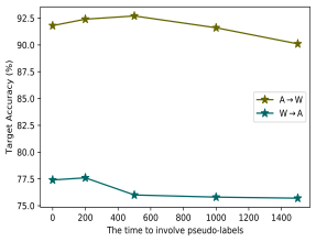
(a) Parameter $I_{s}$

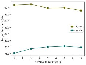
(b) Parameter $K$

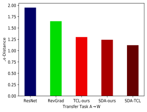
(c) Discrepancy

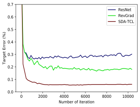
(d) Convergence

Figure 3: Analysis of parameter $I_{s}$, parameter $K$, distribution discrepancy, and convergence.

5.5 Empirical Understanding

The time to involve pseudo-labels. We utilize the parameter $I_{s}$ to control the time to involve the target pseudo-labels in Section 3.2 and we conduct experiments by choosing $I_{s}$ from {0, 200, 500, 1000, 1500} on task A$\rightarrow$W and W$\rightarrow$A. The results shown in Figure 3(a) indicate that there is a trade-off for the time to involve target pseudo-labels and a relative small iteration could be a good choice, which is consistent with the analysis in Section 3.2.

Parameter Sensitivity. In our method SDA-TCL, we use the parameter $K$ to decide $\lambda_{t}$ that controls the importance of utilizing the target pseudo-labels. We conduct experiments to evaluate SDA-TCL by choosing $K$ in the range of {1,3,5,7,9} on task A$\rightarrow$W and W$\rightarrow$A. From the results shown in Figure 3(b), we can find that SDA-TCL can achieve good performance with a wide range of $K$.

Distribution Discrepancy. The $\mathcal{A}$-distance is defined as $\text{dist}_{\mathcal{A}}=2(1-2\epsilon)$ to measure the distribution discrepancy [43, 54], where $\epsilon$ denotes the test error of a classifier trained to discriminate the source from target. A smaller $\text{dist}_{\mathcal{A}}$ means a smaller domain gap. Figure 3(c) shows $\text{dist}_{\mathcal{A}}$ on task A$\rightarrow$W with features of ResNet, RevGrad, SDA-ours, TCL-ours and SDA-TCL. The results indicate that SDA-TCL can reduce the domain gap more effectively. With class-level distribution alignment, SDA-ours and SDA-TCL have a smaller $\text{dist}_{\mathcal{A}}$ than RevGrad. TCL-ours also has a smaller $\text{dist}_{\mathcal{A}}$ than RevGrad, which indicates that TCL-ours is helpful for the domain alignment.

Convergence. We demonstrate the convergence of ResNet, RevGrad, and SDA-TCL, with the error rates in the target domain on task A$\rightarrow$W shown in Figure 3(d). SDA-TCL has faster convergence than RevGrad and the convergence process is more stable than RevGrad.

6 Conclusion

In this paper, we proposed a novel method for unsupervised domain adaptation by jointly optimizing semantic domain alignment and target classifier learning in the feature space. The joint optimization mechanism can not only eliminate their weaknesses but also complement their strengths. Experiments on several benchmarks demonstrate that our method surpasses state-of-the-art unsupervised domain adaptation methods. Recently, learnware is defined to be facilitated with model reusability [55]. The use of a learned model to another task, however, is not trivial. There have been some efforts towards this direction [56, 57, 58, 59], whereas the approach presented in this paper offers another possibility.

References

- [1] Alex Krizhevsky, Ilya Sutskever and Geoffrey E. Hinton “ImageNet Classification with Deep Convolutional Neural Networks” In NIPS, 2012
- [2] Karen Simonyan and Andrew Zisserman “Very Deep Convolutional Networks for Large-Scale Image Recognition” In CoRR abs/1409.1556, 2014
- [3] Christian Szegedy et al. “Going deeper with convolutions” In CVPR, 2015
- [4] Kaiming He, Xiangyu Zhang, Shaoqing Ren and Jian Sun “Deep Residual Learning for Image Recognition” In CVPR, 2016
- [5] Gabriela Csurka “Domain Adaptation for Visual Applications: A Comprehensive Survey” In CoRR abs/1702.05374, 2017
- [6] Eric Tzeng et al. “Deep Domain Confusion: Maximizing for Domain Invariance” In CoRR abs/1412.3474, 2014
- [7] Mingsheng Long, Yue Cao, Jianmin Wang and Michael I. Jordan “Learning Transferable Features with Deep Adaptation Networks” In ICML, 2015
- [8] Baochen Sun and Kate Saenko “Deep CORAL: Correlation Alignment for Deep Domain Adaptation” In ECCV, 2016
- [9] Yaroslav Ganin and Victor S. Lempitsky “Unsupervised Domain Adaptation by Backpropagation” In ICML, 2015
- [10] Eric Tzeng, Judy Hoffman, Kate Saenko and Trevor Darrell “Adversarial Discriminative Domain Adaptation” In CVPR, 2017
- [11] Shaoan Xie, Zibin Zheng, Liang Chen and Chuan Chen “Learning Semantic Representations for Unsupervised Domain Adaptation” In ICML, 2018
- [12] Yingwei Pan et al. “Transferrable Prototypical Networks for Unsupervised Domain Adaptation” In CoRR abs/1904.11227, 2019
- [13] Chaoqi Chen et al. “Progressive Feature Alignment for Unsupervised Domain Adaptation” In CoRR abs/1811.08585, 2018
- [14] Yexun Zhang, Ya Zhang, Yanfeng Wang and Qi Tian “Domain-Invariant Adversarial Learning for Unsupervised Domain Adaption” In CoRR abs/1811.12751, 2018
- [15] Weijian Deng, Liang Zheng and Jianbin Jiao “Domain Alignment with Triplets” In CoRR abs/1812.00893, 2018
- [16] Kuniaki Saito, Yoshitaka Ushiku and Tatsuya Harada “Asymmetric Tri-training for Unsupervised Domain Adaptation” In ICML, 2017
- [17] Weichen Zhang, Wanli Ouyang, Wen Li and Dong Xu “Collaborative and Adversarial Network for Unsupervised domain adaptation” In CVPR, 2018
- [18] Mingsheng Long, Han Zhu, Jianmin Wang and Michael I. Jordan “Deep Transfer Learning with Joint Adaptation Networks” In ICML, 2017
- [19] Yaroslav Ganin et al. “Domain-Adversarial Training of Neural Networks” In Journal of Machine Learning Research 17, 2016, pp. 59:1–59:35
- [20] Pedro Oliveira Pinheiro “Unsupervised Domain Adaptation with Similarity Learning” In CVPR, 2018
- [21] Chao Chen, Zhihong Chen, Boyuan Jiang and Xinyu Jin “Joint Domain Alignment and Discriminative Feature Learning for Unsupervised Deep Domain Adaptation” In CoRR abs/1808.09347, 2018
- [22] Guoliang Kang, Liang Zheng, Yan Yan and Yi Yang “Deep Adversarial Attention Alignment for Unsupervised Domain Adaptation: The Benefit of Target Expectation Maximization” In ECCV, 2018
- [23] Bharath Bhushan Damodaran et al. “DeepJDOT: Deep Joint Distribution Optimal Transport for Unsupervised Domain Adaptation” In ECCV, 2018
- [24] Mingsheng Long, Zhangjie Cao, Jianmin Wang and Michael I. Jordan “Conditional Adversarial Domain Adaptation” In NeurIPS, 2018
- [25] M.-Y. Liu and Oncel Tuzel “Coupled Generative Adversarial Networks” In NIPS, 2016
- [26] Konstantinos Bousmalis et al. “Unsupervised Pixel-Level Domain Adaptation with Generative Adversarial Networks” In CVPR, 2017
- [27] Jun-Yan Zhu, Taesung Park, Phillip Isola and Alexei A. Efros “Unpaired Image-to-Image Translation Using Cycle-Consistent Adversarial Networks” In ICCV, 2017
- [28] Ming-Yu Liu, Thomas Breuel and Jan Kautz “Unsupervised image-to-image translation networks” In NIPS, 2017
- [29] Judy Hoffman et al. “CyCADA: Cycle-Consistent Adversarial Domain Adaptation” In ICML, 2018
- [30] Swami Sankaranarayanan, Yogesh Balaji, Carlos D. Castillo and Rama Chellappa “Generate to Adapt: Aligning Domains Using Generative Adversarial Networks” In CVPR, 2018
- [31] Philip Haeusser, Thomas Frerix, Alexander Mordvintsev and Daniel Cremers “Associative domain adaptation” In ICCV, 2017
- [32] Muhammad Ghifary et al. “Deep Reconstruction-Classification Networks for Unsupervised Domain Adaptation” In ECCV, 2016
- [33] Konstantinos Bousmalis et al. “Domain Separation Networks” In NIPS, 2016
- [34] Kuniaki Saito, Yoshitaka Ushiku, Tatsuya Harada and Kate Saenko “Adversarial Dropout Regularization” In CoRR abs/1711.01575, 2017
- [35] Kuniaki Saito, Kohei Watanabe, Yoshitaka Ushiku and Tatsuya Harada “Maximum Classifier Discrepancy for Unsupervised Domain Adaptation” In CVPR, 2018
- [36] Abhishek Kumar et al. “Co-regularized Alignment for Unsupervised Domain Adaptation” In NeurIPS, 2018
- [37] Mingsheng Long, Han Zhu, Jianmin Wang and Michael I. Jordan “Unsupervised Domain Adaptation with Residual Transfer Networks” In NIPS, 2016
- [38] Geoffrey French, Michal Mackiewicz and Mark Fisher “Self-ensembling for visual domain adaptation” In ICLR, 2018
- [39] Rui Shu, Hung H Bui, Hirokazu Narui and Stefano Ermon “A DIRT-T Approach to Unsupervised Domain Adaptation” In ICLR, 2018
- [40] Ozan Sener, Hyun Oh Song, Ashutosh Saxena and Silvio Savarese “Learning Transferrable Representations for Unsupervised Domain Adaptation” In NIPS, 2016
- [41] Issam H. Laradji and Reza Babanezhad “M-ADDA: Unsupervised Domain Adaptation with Deep Metric Learning” In CoRR abs/1807.02552, 2018
- [42] Jian Liang, Ran He, Zhenan Sun and Tieniu Tan “Aggregating Randomized Clustering-Promoting Invariant Projections for Domain Adaptation” In IEEE Transactions on Pattern Analysis and Machine Intelligence 41.5 IEEE, 2019, pp. 1027–1042
- [43] Shai Ben-David et al. “A theory of learning from different domains” In Machine Learning 79.1-2, 2010, pp. 151–175
- [44] Shai Ben-David, John Blitzer, Koby Crammer and Fernando Pereira “Analysis of Representations for Domain Adaptation” In NIPS, 2006
- [45] Koby Crammer, Michael J. Kearns and Jennifer Wortman “Learning from Multiple Sources” In Journal of Machine Learning Research 9, 2008, pp. 1757–1774
- [46] Kate Saenko, Brian Kulis, Mario Fritz and Trevor Darrell “Adapting Visual Category Models to New Domains” In ECCV, 2010
- [47] Jonathan J. Hull “A Database for Handwritten Text Recognition Research” In IEEE Transactions on Pattern Analysis and Machine Intelligence 16.5, 1994, pp. 550–554
- [48] Yann LeCun, Léon Bottou, Yoshua Bengio and Patrick Haffner “Gradient-based learning applied to document recognition” In Proceedings of the IEEE 86.11 IEEE, 1998, pp. 2278–2324
- [49] Xingchao Peng et al. “VisDA: The Visual Domain Adaptation Challenge” In CoRR abs/1710.06924, 2017
- [50] Olga Russakovsky et al. “ImageNet Large Scale Visual Recognition Challenge” In International Journal of Computer Vision 115.3, 2015, pp. 211–252
- [51] Diederik P. Kingma and Jimmy Ba “Adam: A Method for Stochastic Optimization” In CoRR abs/1412.6980, 2014
- [52] Florian Schroff, Dmitry Kalenichenko and James Philbin “FaceNet: A unified embedding for face recognition and clustering” In CVPR, 2015
- [53] R. Manmatha, Chao-Yuan Wu, Alexander J. Smola and Philipp Krähenbühl “Sampling Matters in Deep Embedding Learning” In ICCV, 2017
- [54] Yishay Mansour, Mehryar Mohri and Afshin Rostamizadeh “Domain Adaptation: Learning Bounds and Algorithms” In COLT, 2009
- [55] Z.-H. Zhou “Learnware: on the future of machine learning” In Frontiers of Computer Science 10.4, 2016, pp. 589–590
- [56] H.-J. Ye, D.-C. Zhan, Y. Jiang and Z.-H. Zhou “Rectify Heterogeneous Models with Semantic Mapping” In ICML, 2018
- [57] Z.Y. Shen and Ming Li “T2S: Domain Adaptation Via Model-Independent Inverse Mapping and Model Reuse” In ICDM, 2018
- [58] Yang Yang et al. “Deep Learning for Fixed Model Reuse” In AAAI, 2017
- [59] Y.-Q. Hu, Y. Yu and Z.-H. Zhou “Experienced Optimization with Reusable Directional Model for Hyper-Parameter Search” In IJCAI, 2018