Note on the bias and variance of variational inference

Abstract

In this note, we study the relationship between the variational gap and the variance of the (log) likelihood ratio. We show that the gap can be upper bounded by some form of dispersion measure of the likelihood ratio, which suggests the bias of variational inference can be reduced by making the distribution of the likelihood ratio more concentrated, such as via averaging and variance reduction.

1 Introduction

Let ${\bm{v}}$ and ${\bm{h}}$ denote the observed and unobserved random variables, following a joint density function $p_{\theta}({\bm{v}},{\bm{h}})$. Generally, the log marginal likelihood $\log p_{\theta}({\bm{v}})=\log\int_{\bm{h}}p_{\theta}({\bm{v}},{\bm{h}})d{\bm{h}}$ is not tractable, so the Maximum likelihood principle cannot be readily applied to estimate the model parameter $\theta$. Instead, one can maximize the evidence lower bound (ELBO):

$$\log p_{\theta}({\bm{v}})=\log\mathbb{E}_{q_{\phi}({\bm{h}})}\left[\frac{p_{\theta}({\bm{v}},{\bm{h}})}{q_{\phi}({\bm{h}})}\right]\geq\mathbb{E}_{q_{\phi}({\bm{h}})}\left[\log\frac{p_{\theta}({\bm{v}},{\bm{h}})}{q_{\phi}({\bm{h}})}\right]:={\mathcal{L}}(\theta,\phi)$$

where the inequality becomes an equality if and only if $q({\bm{h}})=p({\bm{h}}|{\bm{v}})$, since $\log$ is a strictly concave function. This way, learning and inference can be jointly achieved, by maximizing ${\mathcal{L}}(\theta,\phi)$ wrt $\theta$ and $\phi$, respectively.

Alternatively, one can maximize another family of lower bounds due to Burda et al. (2015):

$$\log p_{\theta}({\bm{v}})=\log\mathbb{E}_{{\bm{h}}_{j}\sim q_{\phi}({\bm{h}})}\left[\frac{1}{K}\sum_{j=1}^{K}\frac{p_{\theta}({\bm{v}},{\bm{h}}_{j})}{q_{\phi}({\bm{h}}_{j})}\right]\geq\mathbb{E}_{{\bm{h}}_{j}\sim q_{\phi}({\bm{h}})}\left[\log\frac{1}{K}\sum_{j=1}^{K}\frac{p_{\theta}({\bm{v}},{\bm{h}})}{q_{\phi}({\bm{h}})}\right]:={\mathcal{L}}_{K}(\theta,\phi)$$

which we call the importance weighted lower bound (IWLB). Clearly ${\mathcal{L}}_{1}={\mathcal{L}}$. An appealing property of this family of lower bounds is that ${\mathcal{L}}_{K}$ is monotonic, i.e. ${\mathcal{L}}_{M}\geq{\mathcal{L}}_{N}$ if $M\geq N$, and can be made arbitrarily close to $\log p_{\theta}$ provided $K$ is sufficiently large.

One interpretation for this is that by weighting the samples according to the importance ratio $p/q$, we are effectively correcting or biasing the proposal towards the true posterior $p_{\theta}({\bm{h}}|{\bm{v}})$; see Cremer et al. (2017) for more details. Another interpretation due to Nowozin (2018) is to view $Y_{K}:=\log\frac{1}{K}\sum_{j=1}^{K}\frac{p_{\theta}({\bm{v}},{\bm{h}})}{q_{\phi}({\bm{h}})}$ as a biased estimator for $\log p_{\theta}({\bm{v}})$, where the bias is of the order ${\mathcal{O}}(K^{-1})$.

We take a different view by looking at the variance, or some notion of dispersion, of $Y_{K}$. We write $X_{K}:=\exp(Y_{K})$ as the average before $\log$ is applied. The variational gap, $\log\mathbb{E}[X_{K}]-\mathbb{E}[Y_{K}]$, is caused by (1) the strict concavity of $\log$, and (2) the dispersion of $X_{K}$. To see this, one can view the expectation $\mathbb{E}[Y_{K}]$ as the centroid of uncountably many $\log X_{K}$ weighted by its probability density, which lies below the graph of $\log$. By using a larger number of samples, the distribution of $X_{K}$ becomes more concentrated around its expectation $\mathbb{E}[X_{K}]=\log p_{\theta}({\bm{v}})$, pushing the “centroid” up to be closer to the graph of $\log$. See Figure 1 for an illustration.

This intuition has been exploited and ideas of correlating the likelihood ratios $X=p/q$ of a joint proposal $q({\bm{h}}_{1},...,{\bm{h}}_{K})$ have been proposed in Klys et al. (2018); Wu et al. (2019); Huang et al. (2019). Even though attempts have been made to establish the connection between $\mathrm{Var}(X)$ and the gap (or bias) $\log\mathbb{E}[X]-\mathbb{E}[\log X]$, the obtained results are asymptotic and require further assumption on boundedness (such as uniform integrability) of the sequence $\{X_{n}\}_{n\geq 1}$, which makes the results harder to interpret . Rather than bounding the asymptotic bias by the variance of $X$, we analyze the non-asymptotic relationship between $\log\mathbb{E}[X]-\mathbb{E}[\log X]$ and the variance of $X$ and $\log X$. Our finding justifies exploiting the structure of the likelihood ratios of a joint proposal, as anti-correlation among the likelihood ratio serves to further reduce the variance of an average, which we will show in the next section upper bounds the variational gap.

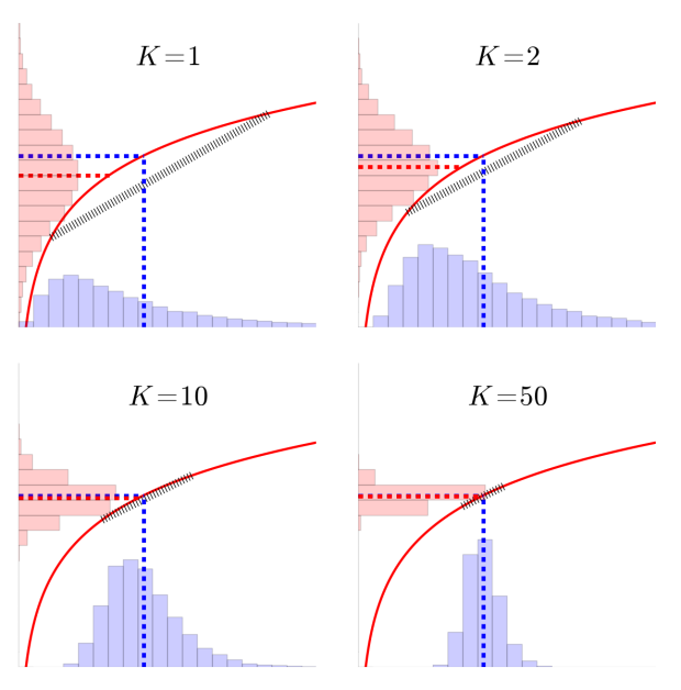
Figure 1: Visualizing the reduction in variaional gap and the concentration of the distribution of the likelihood ratio due to averaging. x-axis: $X_{K}$. y-axis: $Y_{K}$. The dotted lines indicate the expected values, and the solid line is the $\log$ function.

2 Bounding the gap via central tendency

Let $\mu_{X}$ and $\nu_{X}$ be the mean and median of a random variable $X$, i.e.

$$\mu_{X}:=\mathbb{E}[X]\qquad\qquad{\mathbb{P}}(X\geq\nu_{X})\wedge\,{\mathbb{P}}(X\leq\nu_{X})\geq\frac{1}{2}$$

Here we assume $X>0$ is a positive random variable. One can think of it as $p/q$, or some other unbiased estimate of $p({\bm{v}})$. By Jensen’s inequality, we know $\log\mu_{X}\geq\mu_{Y}=\mathbb{E}[\log X]$, where $Y:=\log X$. We want to bound the gap $\log\mu_{X}-\mu_{Y}$ via some notion of dispersion of $X$ and $Y$. Now assume $\mu_{X}-\nu_{X}\leq C_{X}$ and $\mu_{Y}-\nu_{Y}\leq C_{Y}$. Constants $C_{X}$ and $C_{Y}$ correspond to the dispersion just mentioned. For example, the following lemma shows $C_{X}$ can be taken to be the standard deviation $\sigma_{X}:=\sqrt{\mathbb{E}[(X-\mu_{X})^{2}]}$:

Proposition 1.

For $p\geq 1$ and $X\in L_{p}$, then $|\mu_{X}-\nu_{X}|\leq||X-\mu_{X}||_{p}$.

Proof.

Using the fact that the median minimizes the mean absolute error and Jensen’s inequality, we have

$$|\mu_{X}-\nu_{X}|=|\mathbb{E}[X-\nu_{X}]|\leq\mathbb{E}[|X-\nu_{X}|]\leq\mathbb{E}[|X-\mu_{X}|]\leq||X-\mu_{X}||_{p}$$

∎

Without further assumptions, we can derive a weaker result. Since $\log$ is strictly monotonic, $\log\nu_{X}=\nu_{Y}$, so we have $\log\mu_{X}-\mu_{Y}=\log\mu_{X}-\log\nu_{X}+\nu_{Y}-\mu_{Y}$. Since $\nu_{X}\geq\mu_{X}-C_{X}$, by monotonicity of $\log$,

$$\log\mu_{X}-\mu_{Y}\leq\log\mu_{X}-\log(\mu_{X}-C_{X})+\nu_{Y}-\mu_{Y}$$

which after arrangement gives $\log(\mu_{X}-C_{X})-\mu_{Y}\leq\nu_{Y}-\mu_{Y}\leq C_{Y}$. This means if $C_{X}$ is small enough so that the difference between $\log\mu_{X}$ and $\log(\mu_{X}-C_{X})$ can be neglected, then the gap of interest is bounded by the dispersion of $Y$, $C_{Y}$.

Now, we quantify the error between $\log\mu_{X}$ and $\log(\mu_{X}-C_{X})$ by the following result:

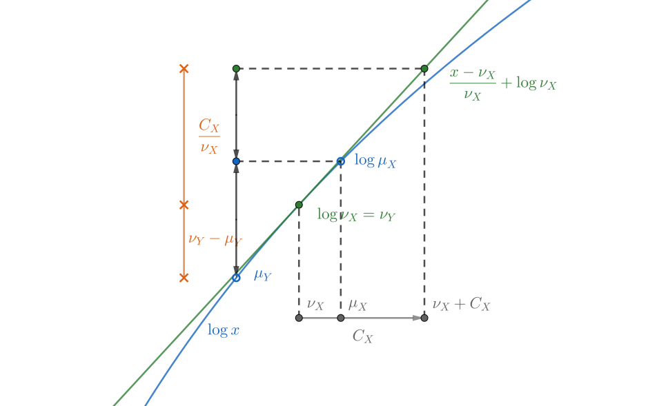
Figure 2: Bounding the variational gap using a linear majorizer (green curve) of $\log$ (blue curve) at $x=\nu_{X}$.

Proposition 2.

Let $X>0$ be a positive random variable with $\mu_{X}=\mathbb{E}[X]$, and $Y=\log X$ with $\mu_{Y}=\mathbb{E}[Y]=\mathbb{E}[\log X]\leq\log\mathbb{E}[X]=\log\mu_{X}$. Assume

$$|\mu_{X}-\nu_{X}|\leq C_{X}\qquad{(*)}\qquad\text{ and }\qquad|\mu_{Y}-\nu_{Y}|\leq C_{Y}\qquad{(\dagger)}$$

for some constants $C_{X},C_{Y}\geq 0$. If $\mu_{X}>C_{X}$, then

$$\log\mu_{X}-\mu_{Y}\leq\frac{C_{X}}{\mu_{X}-C_{X}}+C_{Y}$$

A visual illustration of the proof is presented in Figure 2. The main idea is to use Taylor approximation as a linear upper bound on the $\log$, so that the error in using $\mu_{X}-C_{X}$ to approximate $\mu_{X}$ can be translated to the log scale. Hence the additional term $C_{X}/(\mu_{X}-C_{X})$ is inversely propostional to $\mu_{X}-C_{X}$, i.e. the derivative of $\log$, which is the slope of the linear upper bound.

Proof.

Since $\log$ is a strictly concave function, first-order Taylor approximation (at $\nu_{X}$) gives a linear upper bound:

$$f(x):=\frac{1}{\nu_{X}}(x-\nu_{X})+\log\nu_{X}\geq\log(x)$$

By monotonicity of logarithm and $(*)$, $\log\mu_{X}-\mu_{Y}\leq\log(\nu_{X}+C_{X})-\mu_{Y}$. The logarithm can be bounded from above by the linear upperbound $f(\nu_{X}+C_{X})$, which yields

$$\log\mu_{X}-\mu_{Y}\leq f(\nu_{X}+C_{X})-\mu_{Y}=\frac{C_{X}}{\nu_{X}}+\log\nu_{X}-\mu_{Y}$$

Notice that $\log\nu_{X}=\nu_{Y}$ (since $\log$ is strictly monotonic), so that we can plug in $(\dagger)$. Now the premise $\mu_{X}\geq C_{X}$ combined with $(*)$ again yields $\frac{1}{\nu_{X}}\leq\frac{1}{\mu_{X}-C_{X}}$, concluding the proof. ∎

The main takeaway of the proposition is that if the dispersion of $X$ is sufficiently small, then minimizing the standard deviation of $X$ and $\log X$ amounts to minimizing the gap $\log\mathbb{E}[X]-\mathbb{E}[\log X]$. We summarize it by the following Corollary:

Corollary 3.

Let $X>0$ be an unbiased estimator for the marginal likelihood $p({\bm{v}})$, and let $Y=\log X$. Denote by $\sigma_{X}$ and $\sigma_{Y}$ the standard deviation of $X$ and $Y$, respectively. Then

$$\sigma_{X}<p({\bm{v}})\quad\Longrightarrow\quad\log p({\bm{v}})-\mathbb{E}[\log X]\leq\frac{\sigma_{X}}{p({\bm{v}})-\sigma_{X}}+\sigma_{Y}$$

Acknowledgments

We would like to thank Kris Sankaran for proofreading the note.

References

• Burda et al. (2015) Yuri Burda, Roger Grosse, and Ruslan Salakhutdinov. Importance weighted autoencoders. In International Conference on Learning Representations, 2015.
• Cremer et al. (2017) Chris Cremer, Quaid Morris, and David Duvenaud. Reinterpreting importance-weighted autoencoders. arXiv preprint arXiv:1704.02916, 2017.
• Domke and Sheldon (2018) Justin Domke and Daniel R Sheldon. Importance weighting and variational inference. In Advances in Neural Information Processing Systems, pages 4470–4479, 2018.
• Huang et al. (2019) Chin-Wei Huang, Kris Sankaran, Eeshan Dhekane, Alexandre Lacoste, and Aaron Courville. Hierarchical importance weighted autoencoders. In International Conference on Machine Learning, 2019.
• Klys et al. (2018) Jack Klys, Jesse Bettencourt, and David Duvenaud. Joint importance sampling for variational inference. 2018.
• Maddison et al. (2017) Chris J Maddison, John Lawson, George Tucker, Nicolas Heess, Mohammad Norouzi, Andriy Mnih, Arnaud Doucet, and Yee Teh. Filtering variational objectives. In Advances in Neural Information Processing Systems, pages 6573–6583, 2017.
• Nowozin (2018) Sebastian Nowozin. Debiasing evidence approximations: On importance-weighted autoencoders and jackknife variational inference. In International Conference on Learning Representations, 2018.
• Wu et al. (2019) Mike Wu, Noah Goodman, and Stefano Ermon. Differentiable antithetic sampling for variance reduction in stochastic variational inference. In Artificial Intelligence and Statitics (AISTATS), 2019.