Redundancy-Free Computation Graphs for
Graph Neural Networks

Abstract

Existing graph neural networks (GNNs) use ordinary graph representation that directly connects each vertex in a graph with its neighbors. Each vertex computes its activations by aggregating its neighbors independently, resulting in redundant computation and unnecessary data transfers. In this paper, we propose HAG, a new graph representation that explicitly manages intermediate aggregation results hierarchically, which reduces redundant computation and eliminates unnecessary data transfers. We introduce a cost model to quantitatively evaluate the runtime performance of different HAGs and use novel graph search algorithm to find highly optimized HAGs under the cost model. Our evaluation shows that the HAG representation significantly outperforms the standard graph representations by reducing computation costs and memory accesses for neighborhood aggregations by up to 84% and YY%, and increasing end-to-end training throughput by up to 1.9$\times$, while maintaining the original model accuracy.

1 Introduction

Graph neural networks (GNNs) have shown state-of-the-art performance across a number of tasks with graph-structured data, such as social networks, molecule networks, and webpage graphs [GCN, GraphSAGE, DiffPool, GIN, CNLMF]. GNNs use a recursive neighborhood aggregation scheme — in a GNN layer, each node aggregates its neighbors’ activations from the previous GNN layer and uses the aggregated value to update its own activations. The activations of the final GNN layer are used for prediction tasks, such as node classification, graph classification, or link prediction.

Due to the clustering nature of real-world graphs, different nodes in a graph may share a number of common neighbors. For example, in webpage graphs, different websites under the same domain generally have a number of common links (i.e., neighbors). As another example, in recommender systems, users in the same group may have interests in common items.

However, existing GNN representations do not capture these common neighbors in real-world graphs, leading to redundant and unnecessary computation in both GNN training and inference. In particular, existing GNN representations define computation in each GNN layer with a GNN computation graph (referred to as a GNN-graph). For each node $v$ in the input graph, the GNN-graph includes an individual tree structure to describe how to compute $v$’s activations by aggregating the previous-layer activations of $v$’s neighbors. Figure 1b shows the GNN-graph of the input graph in Figure 1a; for example, for node $A$, its neighbor’s activations $h^{(k-1)}_{B}$, $h^{(k-1)}_{C}$ and $h^{(k-1)}_{D}$ from the layer $k-1$ are aggregated to compute new activations $h^{(k)}_{A}$ for the layer $k$ (see the top portion of Figure 1b). The new activations of the other nodes are computed similarly using the previous activations of their neighbors. Notice that this representation results in redundant computation and data transfers. In this small example, both $\{A,B\}$ and $\{C,D\}$ are aggregated twice. In wider and mlulti-layer GNNs, the redundancies in existing GNN representations account for a significant fraction of all computation.

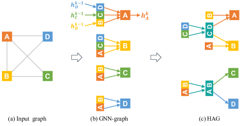
Figure 1: Comparison between a GNN-graph and an equivalent HAG. (a) Input graph; (b) 1-layer GNN computation graph (GNN-graph); (c) HAG that avoids redundant computation. The GNN-graph computes new activations $h^{(k)}_{v}$ by aggregating the previous-layer activations of $v$’s neighbors. Because nodes in the input graph share common neighbors, the GNN-graph performs redundant computation (e.g., both $\{A,B\}$ and $\{C,D\}$ are aggregated twice). (c) By identifying common computational patterns, the HAG avoids repeated computation.

In this paper, we propose a new GNN representation called Hierarchically Aggregated computation Graphs (HAGs). Figure 1c shows one possible HAG for the input graph in Figure 1a. HAGs are functionally equivalent to standard GNN-graphs (produce the same output), but represent common neighbors across different nodes using aggregation hierarchies, which eliminates redundant computation and unnecessary data transfers in both GNN training and inference. In addition, a HAG is agnostic to any particular GNN model, and can be used to eliminate redundancy for arbitrary GNNs.

For a GNN-graph, there exist numerous equivalent HAGs with different aggregation hierarchies and runtime performance. Finding HAGs with optimized performance is challenging since the number of possible HAGs is exponential in the input graph size. We introduce an accurate cost function to quantitatively estimate the performance of different HAGs and develop a novel HAG search algorithm to automatically find optimized HAGs.

Theoretically, we prove that the search algorithm can find HAGs with strong performance guarantees: (1) for GNNs whose neighborhood aggregations require a specific ordering on a node’s neighbors, the algorithm can find a globally optimal HAG under the cost function; and (2) for other GNNs, the algorithm can find HAGs whose runtime performance is at least a $(1-1/e)$ approximation ($\approx 63\%$) of globally optimal HAGs using the submodularity property [mossel2007submodularity]. Empirically, the algorithm finds highly optimized HAGs for real-world graphs, reducing the number of aggregations by up to 6.3$\times$.

Our HAG abstraction maintains the predictive performance of GNNs but leads to much faster training and inference. We evaluate the performance of HAGs on five real-world datasets and along three dimensions: (a) end-to-end training and inference performance; (b) number of aggregations; and (c) size of data transfers. Experiments show that HAGs increase the end-to-end training and inference performance by up to 2.8$\times$ and 2.9$\times$, respectively. In addition, compared to GNN-graphs, HAGs reduce the number of aggregations and the size of data transfers by up to 6.3$\times$ and $5.6\times$, respectively.

To summarize, our contributions are:

• We propose HAG, a new GNN graph representation to eliminate redundant computation and data transfers in GNNs.

• We define a cost model to quantitatively evaluate the runtime performance of different HAGs and develop a HAG search algorithm to automatically find optimized HAGs. Theoretically, we prove that the HAG search algorithm at least finds a $(1-1/e)$-approximation of globally optimal HAGs under the cost model.

• We show that HAGs significantly outperform GNN-graphs by increasing GNN training and inference performance by up to XX$\times$ and YY$\times$, respectively, and reducing the aggregations and data transfers in GNN-graphs by up to 6.3$\times$ and 5.6$\times$, respectively.

2 Related Work

Graph neural networks have been used to solve various real-world tasks with relational structures [GCN, GraphSAGE, DiffPool, GIN, CNLMF]. FastGCN [FastGCN] and SGC [SGC] accelerate GNN training using importance sampling and removing nonlinearilities. This paper solves an orthogonal problem: how to optimize GNN efficiency while maintaining network accuracy. HAG is agnostic to any particular GNN model and provides a general approach that can be automatically applied to eliminate redundancy for arbitrary GNN models.

Join-trees are a tree decomposition technique that maps a graph into a corresponding tree structure to solve optimization problems on the graph, such as query optimization [query_optimization]. Although a join-tree provides a possible way to find optimal HAGs for a GNN-graph, its time complexity is exponential in the treewidth of a GNN-graph [treewidth], and real graphs tend to have very large treewidths. For example, [adcock2016tree] shows that the treewidth of real-world social networks grow linearly with the network size, making it infeasible to use join-trees to find optimal HAGs.

Computation reduction in neural networks.

Several techniques have been proposed to reduce computation in neural networks, including weights pruning [Han1] and quantization [Han2]. These techniques reduce computation at the cost of modifying networks, resulting in decreased accuracy (as reported in these papers). By contrast, we propose a new GNN representation that accelerates GNN training by eliminating redundancy in GNN-graphs while maintaining the original network accuracy.

3 Hierarchically Aggregated Computation Graphs (HAGs)

Table 1: Existing GNNs described in our abstraction. GraphSAGE-P and GraphSAGE-LSTM are the pooling and LSTM variants of GraphSAGE, respectively. $\sigma$ and max indicate element-wise non-linear activation and max functions. For sequential Aggregate, $v_{i}$ denotes the $i$-th in-neighbor of node $v$.

GNN	$\textsc{Aggregate}(\{h^{(k-1)}_{u}|u\in\mathcal{N}(v)\})$	$\textsc{Update}(a^{(k)}_{v},h^{(k-1)}_{v})$
Set Aggregate
GCN [GCN]	$a^{(k)}_{v}=\sum_{u\in\mathcal{N}(v)}{h^{(k-1)}_{u}}$	$h^{(k)}_{v}=\sigma(W^{(k)}\cdot\frac{a^{(k)}_{v}+h^{(k-1)}_{v}}{|\mathcal{N}(v)|+1})$
GraphSAGE-P [GraphSAGE]	$a^{(k)}_{v}={\mbox{\rm\em max}}_{u\in\mathcal{N}(v)}\{\sigma(W^{(k)}_{1}\cdot h^{(k-1)}_{u})\}$	$h^{(k)}_{v}=\sigma\big{(}W^{(k)}_{2}\cdot(a^{(k)},h^{(k-1)}_{v})\big{)}$
Sequential Aggregate
GraphSAGE-LSTM [GraphSAGE]	$a^{(k)}_{v}=\mbox{\rm\em LSTM}(h^{(k-1)}_{v_{1}},...,h^{(k-1)}_{v_{\mathcal{N}}})$	$h^{(k)}_{v}=\sigma\big{(}W^{(k)}\cdot(a^{(k)}_{v},h^{(k-1)}_{v})\big{)}$
$N$-ary Tree-LSTM [TreeLSTM]	$a^{(k)}_{v}=\mbox{\rm\em Tree-LSTM-Agg}(h^{(k-1)}_{v_{1}},...,h^{(k-1)}_{v_{\mathcal{N}}})$	$h^{(k)}_{v}=\mbox{\rm\em Tree-LSTM-Update}(a^{(k)}_{v},h^{(k-1)}_{v})$

Algorithm 1 An abstraction for GNNs. $\mathcal{V}$ is the set of nodes in an input graph, and $\mathcal{N}(v)$ denotes the set of neighbors for node $v$.

1:$h^{(0)}_{v}=x_{v},\forall v\in\mathcal{V}$

2:for $k=1\textrm{ to }K$ do

3:     for $v\in{\mathcal{V}}$ do

4:         $a^{(k)}_{v}\leftarrow\textsc{Aggregate}(\{h^{(k-1)}_{u}|u\in\mathcal{N}(v)\})$

5:         $h^{(k)}_{v}\leftarrow\textsc{Update}(a^{(k)}_{v},h^{(k-1)}_{v})$      

6:

7:Goal: minimize $\mathcal{L}(\{h^{(K)}_{v}|v\in\mathcal{V}\})$

GNN abstraction.

A GNN takes an input graph and node features as inputs and iteratively learns representations for individual nodes over the entire graph through a number of GNN layers. Algorithm 1 shows an abstraction for GNNs: $h^{(k)}_{v}$ is the learned activations of node $v$ at layer $k$, and we initialize $h^{(0)}_{v}$ with input node features $x_{v}$. At the $k$-th layer, $a^{(k)}_{v}$ denotes the aggregated activations of $v$’s neighbors, which is combined with $h^{(k-1)}_{v}$ to compute an updated activation $h^{(k)}_{v}$. The learned node activations of the final layer (i.e., $h^{(K)}_{v}$) are used for predictions, and a GNN model generally minimizes a loss function $\mathcal{L}$ that takes the final node activations as inputs (line 6).

Existing GNN models use a GNN computation graph (GNN-graph) to describe the computation in each GNN layer, as shown in Figure 1b. For each node $v$ in the input graph, the GNN-graph includes an individual tree structure to define how to compute the activations $h_{v}^{(k)}$ of node $v$ by aggregating the previous-layer activations of $v$’s neighbors (i.e., $h^{(k-1)}_{u},u\in\mathcal{N}(v)$). GNN-graphs are efficient at expressing direct neighborhood relations between nodes, but are not capable of capturing common neighbors across multiple nodes, leading to redundant computation in GNN training and inference.