The biasing phenomenon

Abstract

Context. We study biasing as a physical phenomenon by analysing geometrical and clustering properties of density fields of matter and galaxies.

Aims. Our goal is to determine the bias function using a combination of geometrical and power spectrum analysis of simulated and real data.

Methods. We apply an algorithm based on local densities of particles, $\delta$, to form simulated biased models using particles with $\delta\geq\delta_{0}$. We calculate the bias function of model samples as functions of the particle density limit $\delta_{0}$. We compare the biased models with Sloan Digital Sky Survey (SDSS) luminosity limited samples of galaxies using the extended percolation method. We find density limits $\delta_{0}$ of biased models, which correspond to luminosity limited SDSS samples.

Results. Power spectra of biased model samples allow to estimate the bias function $b(>L)$ of galaxies of luminosity $L$. We find the estimated bias parameter of $L_{\ast}$ galaxies, $b_{\ast}=1.85\pm 0.15$.

Conclusions. The absence of galaxy formation in low-density regions of the Universe is the dominant factor of the biasing phenomenon. Second largest effect is the dependence of the bias function on the luminosity of galaxies. Variations in gravitational and physical processes during the formation and evolution of galaxies have the smallest influence to the bias function.

1 Introduction: biasing as a physical phenomenon

The formation of galaxies is very complex including gravitational and hydrodynamical processes. On small scales hydrodynamical processes dominate, on large scales gravitational processes. Thus the biasing phenomenon can be divided into local bias and large-scale bias, as emphasised in the very detailed review by Desjacques et al. (2018). Most papers cited by Desjacques et al. (2018) were devoted to the study of the local bias. In this paper we are interested in the global bias phenomenon, where gravitational processes dominate.

To quantify the large-scale galaxy bias various statistical tools were applied as the galaxy autocorrelation function, starting from Kaiser (1984), Bardeen et al. (1986) and Szalay (1988). Another statistic used to study the relationship between matter and galaxies is the void probability function (VPF), as done by Gramann (1990), Einasto et al. (1991) and more recently by Walsh & Tinker (2019). Presently the power spectrum analysis has been preferred. The power spectrum analysis has several advantages over the correlation function analysis (Feldman et al., 1994). The power spectrum measures the fractional density contributions on different scales, and is a natural quantity to describe the density field, especially on large scales.

Different authors used different data and different methods to the estimation of power spectra, which led to various definitions of the bias parameter. Geometrical properties of the distribution of galaxies and matter were discussed separately using a large variety of methods. This area of research is very rich, as seen from discussions on the recent symposium of cosmic web (van de Weygaert et al., 2016). The connection of determinations of power spectra with geometrical properties of the cosmic web were discussed rarely.

In the present paper we try to get a more general view of the biasing phenomenon in the context of structure of the cosmic web. Biasing phenomenon is a physical problem of the relation between distributions of matter and galaxies on large scales. In discussing the biasing phenomenon we assume that gravity is the dominating force which determines the formation and evolution of the cosmic web on large scales. According to the presently accepted $\Lambda$ cold dark matter ($\Lambda$CDM) model the primordial density field forms a statistically homogeneous, isotropic and almost-Gaussian random field. Density waves of different scales began with random and uncorrelated spatial phases. As the density waves evolve, they interact with others in a non-linear way. This interaction leads to the generation of non-random and correlated phases which form the spatial pattern of the present cosmic web with clusters, filaments, sheets and voids. Matter flows out from under-dense regions towards over-dense regions, which changes the pattern of the evolving cosmic web. In high-density regions there exists conditions favourable for the formation of galaxies.

We consider the bias function $b$ as a fundamental cosmological function, which relates quantitatively differences between distributions of matter and galaxies. The numerical value of the bias function can be found by the power spectrum analysis, the relation between galaxies and matter can be found using geometrical properties of the cosmic web. We discuss first shortly basic physical processes involved in the biasing phenomenon: the formation of galaxies in the cosmic web, the phase synchronisation of density perturbations, and the evolution of voids.

1.1 Formation of the biasing concept

An important element of the classical version of the cosmology paradigm is the distribution of galaxies. Available data on the distribution of galaxies on sky suggested that this distribution is essentially a random one (field galaxies) to which some clusters and perhaps even superclusters were added, see the angular distribution of the numbers of galaxies brighter than $B\approx 19$ by Seldner et al. (1977). The angular distribution of galaxies can be considered as a random Gaussian process, and described by the angular correlation function of galaxies, as done by Peebles (1973), Peebles & Hauser (1974), Peebles & Groth (1975) and Davis & Peebles (1983).

In 1970s the number of galaxies with measured redshifts was sufficiently large to study the distribution of galaxies in three dimensions. The topic was discussed in the IAU Symposium 79 “Large Scale Structure of the Universe” in Tallinn by Jõeveer & Einasto (1978), Tarenghi et al. (1978), Tifft & Gregory (1978) and Tully & Fisher (1978). Three-dimensional data demonstrated that the distribution of galaxies and clusters of galaxies is filamentary and that there are almost no galaxies outside filaments. A theory of the formation of galaxies due to gravitational instability was suggested by Zeldovich (1970). Numerical simulations in the framework of this model by Doroshkevich et al. (1980) demonstrated the formation of a cellular network of high- and low-density regions. Due to the similarity of the observed large-scale distribution of galaxies to the structure, found in simulations, the structure was called “cellular” (Jõeveer et al., 1977, 1978). Subsequently more general terms “supercluster-void network” (Einasto et al., 1980) and “cosmic web” (Bond et al., 1996) were used.

Jõeveer et al. (1977, 1978) estimated that knots, filaments and sheets fill only about one per cent of the whole volume of the universe, the rest forms voids. Authors noticed that gravity works very slowly and it is very unlikely to evacuate completely such large volumes as cell interiors: there must exist unclustered matter in voids. In this way the difference between distributions of matter and galaxies was detected. The structure of superclusters and voids was investigated quantitatively by Zeldovich et al. (1982) by comparing distributions of simulated particles with real galaxies. The multiplicity test confirmed the existence of a smooth population of void particles in simulations. The multiplicity test also showed the absence of a large low-density population of void galaxies in the observed sample. To explain these differences Zeldovich et al. (1982) assumed that the matter density in voids and sheets is too small to start galaxy formation. The term “biasing” was suggested later by Kaiser (1984) to note the difference between correlation functions of clusters of galaxies in respect to galaxies. Subsequently this term was used in a more general case to denote differences in the distribution of galaxies and matter (Davis et al., 1985).

1.2 Formation of galaxies in the web

Galaxy formation is a two-stage process — gravitating material in the Universe condenses first into DM halos (White & Rees, 1978). To form a galaxy, the density of matter must exceed a critical value, the Press-Schechter limit (Press & Schechter, 1974). This result is confirmed by hydrodynamical models of galaxy formation (for early model see Cen & Ostriker, 1992). The arguments by White and Rees are supported by direct observational evidence — all galaxies are DM dominated, especially dwarf galaxies (McConnachie, 2012). The luminous content of galaxies results from the combined action of gravitational and hydrodynamical processes within potential wells provided by the DM .

Arguments by Zeldovich, White and Rees lead to a simple biasing model, where galaxies do not form in low-density regions at all, or are too faint, to be included into flux-limited galaxy surveys.

1.3 Phase synchronisation

The expansion of the Universe in its early phase is an adiabatic process (Zeldovich, 1970; Peebles, 1982b). The growth of adiabatic perturbations proceeds at a low temperature of the primordial “gas”, and the flow of particles is very smooth (Zeldovich, 1970, 1978; Zeldovich et al., 1982). Smooth initial perturbations develop into the non-linear stage and dense regions will be built up by the concentration of matter into caustics by intersection of particle trajectories (Zeldovich, 1978; Zeldovich et al., 1982; Arnold et al., 1982). In this way the skeleton of the cellular cosmic web is formed. First three-dimensional numerical simulation by Doroshkevich et al. (1982) showed only the formation of very large systems with bulky connections without a web of fine filaments. This simulation was made under the assumption that DM is made of massive neutrinos, this is the hot dark matter (HDM) model. Weakly interacting massive particles, called cold dark matter (CDM), were suggested by Peebles (1982a). Quantitative analysis of a CDM model by Melott et al. (1983) showed that the CDM model is in good agreement with observations. In particular, all quantitative tests, applied to the HDM model by Zeldovich et al. (1982), showed that the CDM model is in good agreement with observed samples of galaxies. In the CDM model the intersection of particle trajectories leads directly to the early formation of thin filaments and knots, as shown by Melott et al. (1983), and subsequently studied in more detail by White et al. (1987), Kofman et al. (1990) and Bond et al. (1996).

When the presence of voids was discovered, Dekel & Silk (1986) assumed that voids can be populated with dwarf galaxies. However, observations suggested that voids are marked by the absence of both normal and dwarf galaxies (Einasto et al., 1989; Lindner et al., 1995, 1996; Peebles, 2001; Tinker et al., 2006).

The absence of dwarf galaxies in voids has a simple explanation. The growth of density perturbations is an acoustic phenomenon and can be studied by the wavelet technique (Einasto et al., 2011a, b). Voids are regions in space where due to phase synchronisation medium- and large-scale density waves combine in similar under-density phases. Here the growth of all small-scale density perturbations, responsible for the formation of galaxies, is suppressed. Small-scale density perturbations form initially everywhere, but in regions of under-dense phases of large and medium perturbations the density contrast of small-scale perturbations decreases during the evolution. Galaxies, clusters and superclusters form in regions where medium- and large-scale density waves combine in similar over-density phases. Near maxima of large-scale density perturbations medium and small-scale perturbations grow. This leads to the formation of numerous halos and subhalos around the high- and medium-density peaks. It is possible that just the phase synchronisation leads to the formation of galaxy systems with centrally located giant galaxies surrounded by dwarf galaxies. The formation of satellite galaxies and relations between satellite and main galaxies is presently a subject of intensive studies, both observational and theoretical; for a recent review see Wechsler & Tinker (2018).

1.4 Evolution of voids

Gravity works slowly and there exist always particles which are more-or-less smoothly distributed in low-density regions. Sheth & van de Weygaert (2004), Rieder et al. (2013) and Aragon-Calvo et al. (2016) among others investigated how galaxies form and evolve inside the cosmic web. Galaxies accrete star-forming gas at early times via the network of primordial filaments. The flow of gas along filaments continues. It is evident, that not all matter in filaments (and walls) is presently located in halos — the process is still going on. Density distributions of SDSS samples can be compared with density distributions models. Cautun et al. (2014), Falck & Neyrinck (2015) and Ganeshaiah Veena et al. (2019) highlighted regions belonging to simulated voids, walls, filaments and halos. In all models there exists large under-dense regions, where halo (and thus galaxy) formation is not possible. These studies suggest that the fraction of particles in low-density regions, not associated with halos, is about 25 - 30 % of all particles. This non-clustered matter forms a more-or-less uniformly distributed medium, part of it is located in weak filaments of dark and baryonic matter (Aragon-Calvo et al., 2010).

1.5 Goal of the present paper

The goal of this paper is study biasing as a physical phenomenon and to estimate the bias function using clustering and geometrical properties of the distribution of DM and galaxies. We divide this task to three subtasks: (i) the generation of biased model distributions of matter and the study of geometrical properties of the distribution of DM, simulated and real galaxies; (ii) the calculation of power spectra of simulated biased models and the determination of the bias function using simulated biased models; (iii) the comparison of geometrical properties of simulated and real galaxy samples to find the simulated model which best represents the observed distribution. In simulations full data on the distribution of particles, selection and boundary effects etc. are known, and the comparison of biased and full models is fully differential. As a result of the comparison we find the relation between the biased model selection parameter and galaxy sample selection parameter. The bias function is a function of the selection parameter, used to define biased models to simulate galaxies. This method circumvents the main difficulty of the power spectrum analysis of the biasing phenomenon: from observations we can determine the power spectrum directly only for galaxies of various luminosity, but not for matter. Following this idea we have to decide: (i) how to construct biased model samples, and (ii) how to compare biased models with observations.

We shall use a simple biased DM simulation model and divide matter into a low-density population with no galaxy formation or populated with galaxies below a certain luminosity limit, and to a high-density population with clustered matter, associated with galaxies above the luminosity limit. From observations we get information on the distribution of galaxies at the present epoch (actually the mean age of our observational SDSS sample corresponds to age at redshift $z=0.1$). Following this consideration we use present-day (Eulerian) particle local densities, $\delta$, and label each particle with this density value. Halos surrounding galaxies like our own Galaxy and M31 have an effective radius of the order of 1 $h^{-1}$ Mpc (Einasto et al., 1974a; Karachentsev et al., 2002). Inside such halos hydrodynamical processes leading to the formation of visible galaxies are dominant. In our study we shall use density fields with the size of individual cells 1 $h^{-1}$ Mpc, thus all the details of galaxy formation are hidden inside cells. Local density is expressed in mean density units of the sample. It is a dimensionless quantity and independent on particle mass and galaxy luminosity.

We apply a sharp particle density limit, $\delta_{0}$. Biased model samples include particles with density labels, $\delta\geq\delta_{0}$. These samples are found from the full DM sample by exclusion particles of density labels less than the limit $\delta_{0}$. In this way biased model samples mimic observed samples of galaxies, where there are no galaxies fainter than a certain luminosity limit. We use a series of particle density limits $\delta_{0}$ to find limits, which correspond in the best way to observational samples of galaxies.

To investigate geometrical properties of the cosmic web and to compare models with observations we apply the extended percolation analysis, developed by Einasto et al. (1986), Einasto & Saar (1987) and Einasto et al. (2018). The extended percolation analysis is aimed to describe geometrical properties of the whole cosmic web. It is a complementary to methods which aims are descriptions of properties of elements of the cosmic web, such as knots, filaments, sheets and voids. The extended percolation method allows the comparison of samples with very different border configurations, such as observational samples with conical shell borders and cubic model samples. The extended percolation analysis uses for comparison completely different properties of the cosmic web than the power spectrum analysis, and is suitable to find proper biased models for comparison with observational data.

As a basic reference model sample we use a numerical simulations of the evolution of the web applying $\Lambda$CDM cosmology in a box of size 512 $h^{-1}$ Mpc, almost equal in volume to the volume of the flux-limited SDSS main galaxy survey, (509 $h^{-1}$ Mpc)³ (Liivamägi et al., 2012). We use cosmological parameters: Hubble parameter $H_{0}=100h$ km s^-1 Mpc^-1, matter density parameter $\Omega_{\mathrm{m}}=0.28$, and dark energy density parameter $\Omega_{\Lambda}=0.72$. For comparison we also use halo mass selected samples from the Horizon Run 4 (HR4) simulation by Kim et al. (2015) in a box of size $512$ $h^{-1}$ Mpc. As observational data we shall use absolute magnitude (volume) limited SDSS samples with limits $M_{r}-5\log h=-18.0,\leavevmode\nobreak\ -19.0,\leavevmode\nobreak\ -20.0,\leavevmode\nobreak\ -21.0$.

The paper is organised as follows. In the next Section we describe the calculation of the density fields of observed and simulated samples, and the method to find clusters, voids and their parameters. In Section 3 we investigate geometrical properties of the cosmic web as delineated by matter and galaxies using the extended percolation method. In Section 4 we calculate power spectra and estimate the bias function of model samples. In Section 5 we compare observed and simulated clusters and voids, and find biased models which correspond to luminosity selected SDSS galaxies in the best way. In Section 6 we discuss our results. The last Section brings our main conclusions.

2 Data and methods

2.1 Particle density selected model samples

Simulations of the evolution of the cosmic web were performed in a box of size $L_{0}=512$ $h^{-1}$ Mpc, with resolution $N_{\mathrm{grid}}=512$ and with $N_{\mathrm{part}}=N_{\mathrm{grid}}^{3}$ particles. The initial density fluctuation spectrum was generated using the COSMICS code by Bertschinger (1995), assuming cosmological parameters $\Omega_{\mathrm{m}}=0.28$, $\Omega_{\Lambda}=0.72$, $\sigma_{8}=0.84$, and the dimensionless Hubble constant $h=0.73$. To generate initial data we used the baryonic matter density $\Omega_{\mathrm{b}}=0.044$ (Tegmark et al. (2004b)). Calculations were performed with the GADGET-2 code by Springel (2005).

The accepted $\sigma_{8}$ for the model is in good agreement with $\sigma_{8}$ determinations for matter, see Planck Collaboration et al. (2018) for Planck 2018 results. Spectra of CMB temperature and polarisation in combination with CMB gravitational lensing yield $\sigma_{8}=0.8111\pm 0.0060$. If data on BAO at lower redshifts is added, then the result is $\sigma_{8}=0.8102\pm 0.0060$. Zubeldia & Challinor (2019) derived cosmological constraints using Planck sample of clusters, detected via the Sunyaev-Zeldovich (SZ) effect. Authors find $\sigma_{8}=0.76\pm 0.04$. The signal from CMB comes from redshift $z=1100$, SZ clusters have characteristic redshift $z\approx 0.2$. Thus data from different distances are in very good agreement.

Table 1: L512 particle density limited models.

Sample	$\delta_{0}$	$F_{C}$	$FF_{C}$	$b(\delta_{0})$
(1)	(2)	(3)	(4)	(5)
L512.00	0.0	1.000	1.0000	1.000
L512.05	0.5	0.901	0.5163	1.199
L512.1	1.0	0.797	0.3434	1.302
L512.2	2.0	0.678	0.2159	1.429
L512.5	5.0	0.516	0.10743	1.635
L512.7	7.5	0.449	0.07665	1.740
L512.10	10.0	0.4036	0.05972	1.820
L512.15	15.0	0.3435	0.04138	1.943
L512.20	20.0	0.3011	0.03146	2.039
L512.50	50.0	0.1831	0.01169	2.432
L512.100	100.0	0.1046	0.00467	2.970

We calculated for all simulation particles and all simulation epochs local density values at particle locations, $\delta$, using positions of 27 nearby particles. Densities were expressed in units of the mean density of the whole simulation. In this paper we used particle density selected samples at the present epoch. Biased model samples contain particles above a certain limit, $\delta\geq\delta_{0}$, in units of the mean density of the simulation. For the analysis we used density limits $\delta_{0}=0.5,\leavevmode\nobreak\ 1.0,\leavevmode\nobreak\ 2.0,\leavevmode\nobreak\ 5.0,\leavevmode\nobreak\ 7.5,\leavevmode\nobreak\ 10.0,\leavevmode\nobreak\ 15.0,\leavevmode\nobreak\ 20.0,\leavevmode\nobreak\ 50.0,\leavevmode\nobreak\ 100.0$. Particle density selected samples are called biased model samples and are denoted as L512.$i$, where $i$ denotes the particle density limit $\delta_{0}$. The full DM model includes all particles and corresponds to particle density limit $\delta_{0}=0$, thus it is denoted as L512.00. Main data on biased model samples are given in Table 1. We give in the Table also the fraction of particles, $F_{C}=N_{C}/N_{\mathrm{part}}$, where $N_{C}$ is the number of particles with density limit $\delta\geq\delta_{0}$, and $N_{\mathrm{part}}$ is the total number of particles in simulation. $F_{C}$ is equal to the number density of selected particles, $\delta\geq\delta_{0}$, per cubic $h^{-1}$ Mpc, $Dens$. We give also the total filling factor of over-density regions at density threshold $D_{t}=0.1$, $FF_{C}$, and the bias parameters $b(\delta_{0})$, calculated using Eq. (3) below.

The use of the local density as the only parameter to determine the fate of particles in the web is a simplification, see the distribution of particles in regions of different density by Cautun et al. (2014) and Ganeshaiah Veena et al. (2019). However, as shown among others by Tinker & Conroy (2009), just the local density, not the global one, is essential in the determination of the formation of galaxies inside DM haloes. In observational SDSS samples and comparison HR4 model samples we used sharp limits of absolute magnitudes and halo masses. The formation of galaxies inside DM halos is determined by a variety of processes. For this reason particles of slightly various densities can be located in halos of fixed lower mass limit and the actual particle density limit is fuzzy. To take this effect into account we made additional calculations with L512 models with fuzzy particle density limits, see below.

2.2 Luminosity limited SDSS galaxy samples

We use luminosity limited (usually called volume-limited) galaxy samples by Tempel et al. (2014), selected from the data release DR10 of the SDSS galaxy redshift survey (Ahn et al., 2014). Data on four luminosity limited SDSS samples are given in Table 2. Limiting absolute magnitudes in red $r-$band, $M_{r}$, maximum comoving distances, $d_{\mathrm{lim}}$, and numbers of galaxies in samples, $N_{\mathrm{gal}}$, are taken from Tempel et al. (2014); volumes of samples, $V_{0}$, and sample lengths, $L_{0}$, are determined by counting cells inside the conical survey volume, and the maximum lengths of over-density regions (clusters in our terminology). SDSS samples with $M_{r}-5\log h$ luminosity limits $-18.0$, $-19.0$, $-20.0$, and $-21.0$ are called SDSS.18, SDSS.19, SDSS.20 and SDSS.21. Respective luminosity limits in Solar units were calculated using the absolute magnitude of the Sun in $r-$band, $M_{\odot}=4.64$ (Blanton & Roweis, 2007). We give in the Table also the number density of sample galaxies per cubic $h^{-1}$ Mpc, $Dens$. SDSS galaxy samples are conical and have different sizes: the volume of the sample SDSS.21 is 52 times larger than the volume of the sample SDSS.18.

Table 2: SDSS luminosity limited samples.

Sample	$M_{r}$	$d_{\mathrm{lim}}$	$L_{0}$	$V_{0}$	$N_{\mathrm{gal}}$	$Dens$
(1)	(2)	(3)	(4)	(5)	(6)	(7)
SDSS.18	$-18.0$	135	243	$117^{3}$	49 860	0.0311
SDSS.19	$-19.0$	211	379	$188^{3}$	105 041	0.0158
SDSS.20	$-20.0$	323	581	$290^{3}$	163 094	0.00669
SDSS.21	$-21.0$	486	865	$438^{3}$	125 016	0.00149

2.3 Halo mass limited model samples

To check the comparison of observed and biased model data we applied the extended percolation analysis also for a series of halo mass limited model samples, taken from the Horizon Run 4 simulation by Kim et al. (2015). This simulation was made in a cubic box of size $3150$ $h^{-1}$ Mpc, using $6300^{3}$ particles, in a $\Lambda$CDM cosmology with $\Omega_{m}=0.26$, $\Omega_{b}=0.044$, $\Omega_{\Lambda}=0.74$, amplitude parameter $\sigma_{8}=0.794$, and current Hubble expansion constant $H_{0}=100h$ km/s/Mpc, where $h=0.72$. We selected from this simulation halos for the present epoch in a box of size $L_{0}=512$ $h^{-1}$ Mpc. Halos were found containing at least 30 particles, minimal mass of halos is $M_{s}=2.706\times 10^{11}$ $h^{-1}M_{\odot}$. This simulation contains 8 particles per cell of length 1 $h^{-1}$ Mpc, mean density of matter per cell is $M_{mean}=0.7216\times 10^{11}$ $h^{-1}M_{\odot}$. We use four halo mass limited samples from HR4 simulation. Main data on HR4 samples are given in Table 3. We give in the Table also the fraction of mass in the clustered population, $F_{C}$, and the number density of halos per cubic $h^{-1}$ Mpc, $Dens$.

Table 3: HR4 halo mass limited samples.

Sample	$M_{h}$	$N_{\mathrm{halo}}$	$F_{C}$	$Dens$
(1)	(2)	(3)	(4)	(5)
HR4.11	$2.71\times 10^{11}$	1 561 724	0.3729	0.01164
HR4.12	$1.00\times 10^{12}$	254 067	0.3184	0.00189
HR4.123	$3.00\times 10^{12}$	223 653	0.2659	0.00166
HR4.13	$1.00\times 10^{13}$	53 484	0.2011	0.00040

2.4 Calculation of percolation functions

The first step in the extended percolation analysis is the calculation of density fields. Here we applied the $B_{3}$ spline (see Martínez & Saar, 2002). This function is different from zero only in the interval $x\in[-2,2]$. To calculate the high-resolution density field we use the kernel of the scale, equal to the cell size of the simulation, $L_{0}/N_{\mathrm{grid}}=1$ $h^{-1}$ Mpc, where $L_{0}$ is the size of the simulation box, and $N_{\mathrm{grid}}$ is the number of grid elements in one coordinate. The smoothing with index $i$ has a smoothing radius $r_{i}=L_{0}/N_{\mathrm{grid}}\times 2^{i}$. The effective scale of smoothing is equal to $r_{i}$. We applied this smoothing up to index 6. For our L512 model smoothing indexes $i=1$, 2 and 3 correspond to $B_{3}$ kernels of radii $R_{B}=2$, 4 and 8 $h^{-1}$ Mpc, respectively. The $B_{3}$ kernel of radius $R_{B}=1$ $h^{-1}$ Mpc corresponds to a Gaussian kernel with dispersion $R_{G}=0.6$ $h^{-1}$ Mpc (Tempel et al., 2014). Non-smoothed density field corresponds to kernel $R_{B}=1$ $h^{-1}$ Mpc. Densities were expressed in mean density units.

The calculation of percolation functions consists of several steps. We scanned density fields in a range of threshold densities from $D_{t}=0.1$ to $D_{t}=10$ in mean density units to find over- and under-density systems, called clusters and voids, respectively. We used a logarithmic step of densities, $\Delta\log D_{t}=0.02$. Two cells of the same type are considered as members of a system if they have a common sidewall. For each cluster and void we calculate the centre coordinates, $x_{c},y_{c},z_{c}$ (mean values of extreme $x,y,z$ coordinates); sizes along coordinate axes, $\Delta x,\leavevmode\nobreak\ \Delta y,\leavevmode\nobreak\ \Delta z$ (differences between extreme $x,y,z$ coordinates); geometrical diameters, $L_{\mathrm{geom}}=\sqrt{(\Delta x)^{2}+(\Delta y)^{2}+(\Delta z)^{2}}$; maximal sizes along coordinate axes, $L_{\mathrm{max}}=\max(\Delta x,\Delta y,\Delta z)$; volumes, $V_{C}$, defined as the volume of space where the density is equal or greater than the threshold density $D_{t}$; total masses (or luminosities), $M_{t}$, i.e. the masses (luminosities) inside the density contour $D_{t}$ of the cluster, both in mean density units.

During the cluster search we found the cluster with the largest volume for the given threshold density, and stored for each threshold density the number of clusters found, and data on the largest cluster: the geometrical diameter (the maximal size along coordinate axes), the volume, and the total mass (luminosity). Diameters (lengths) of largest clusters, ${L}(D_{t})=L_{\mathrm{max}}$, filling factors of largest clusters, $\mathcal{F}(D_{t})=V_{\mathrm{max}}/V_{0}$, and numbers of clusters at the threshold density, $\mathcal{N}(D_{t})$, as functions of the threshold density, $D_{t}$, were used as percolation functions. Diameters are expressed in $h^{-1}$ Mpc, volumes (actually the filling factors) are expressed in units of the volume of the whole sample, $V_{0}$. During the search of high- and low-density systems we excluded very small systems, using exclusion volume limit, $N_{\mathrm{lim}}=50$ or 500 computation cells (cubic $h^{-1}$ Mpc). Length functions ${L}(D_{t})$ and filling factor functions $\mathcal{F}(D_{t})$ are not influenced by the choice of $N_{\mathrm{lim}}$.

We use as a percolation function the volume of the largest cluster, $V_{\mathrm{max}}$, not its mass, $M_{\mathrm{max}}$. The mass function depends on the mass concentration inside halos. The volume is free from this dependence, here the question is whether the cluster lies above or below the limit dividing particles or halos to over- and under-dense regions. This aspect is treated by the fuzziness of the particle selection limit.

A similar procedure was applied to find the largest low-density regions or voids in our terminology.

3 Geometrical properties of density fields of matter and galaxies

In this Section we compare distributions of matter and galaxies using the extended percolation method. We pay special attention to similarities and differences between distributions of DM and galaxies, both simulated and real.

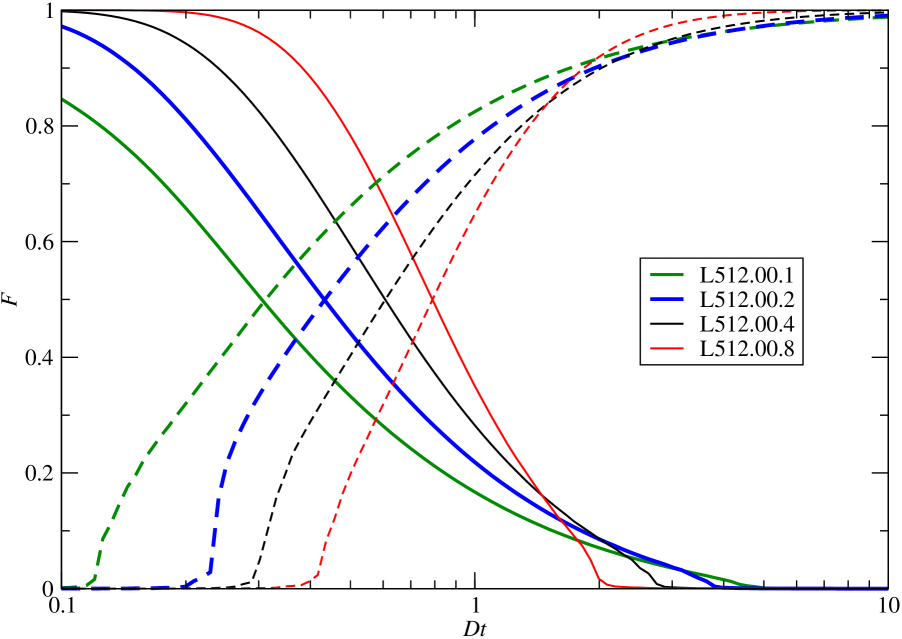
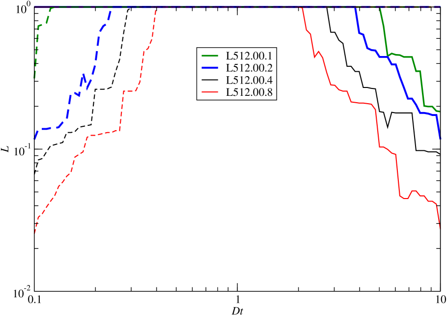
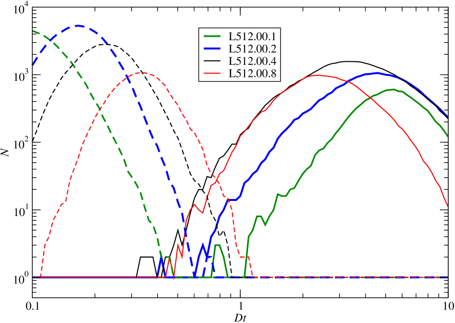
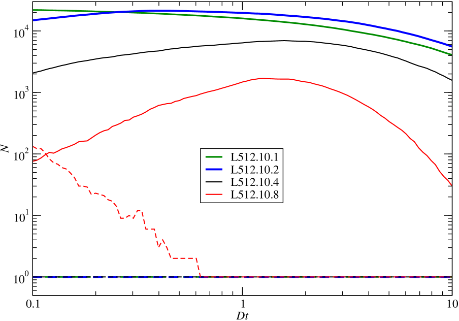
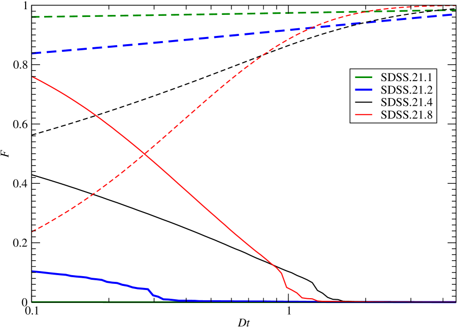
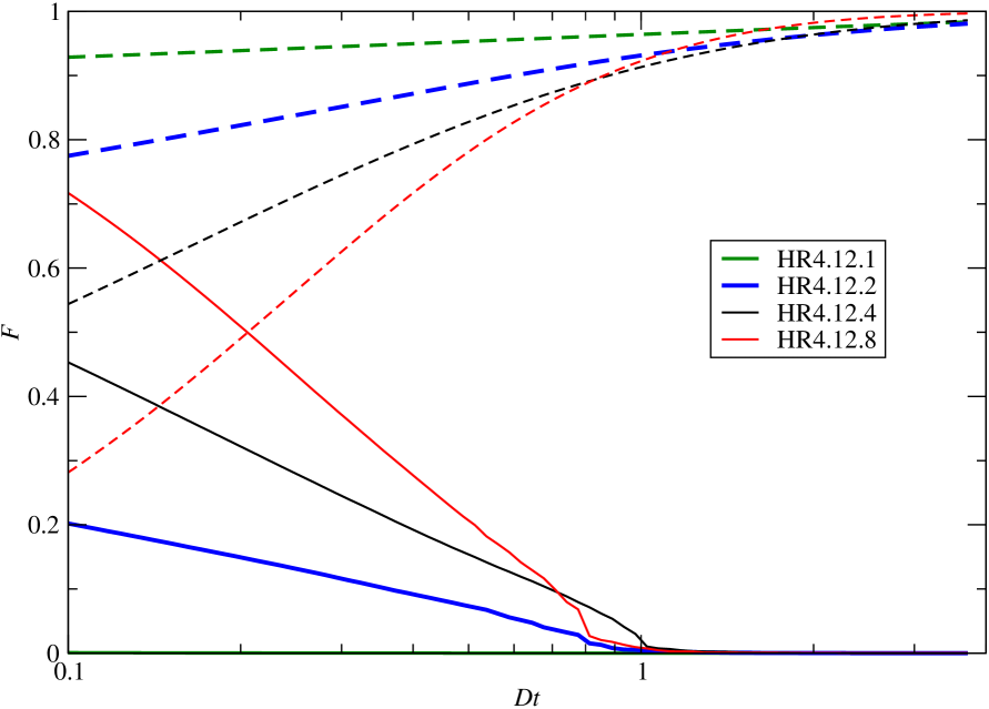
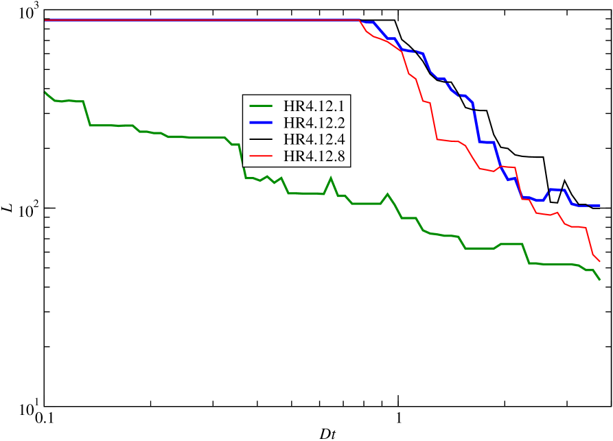
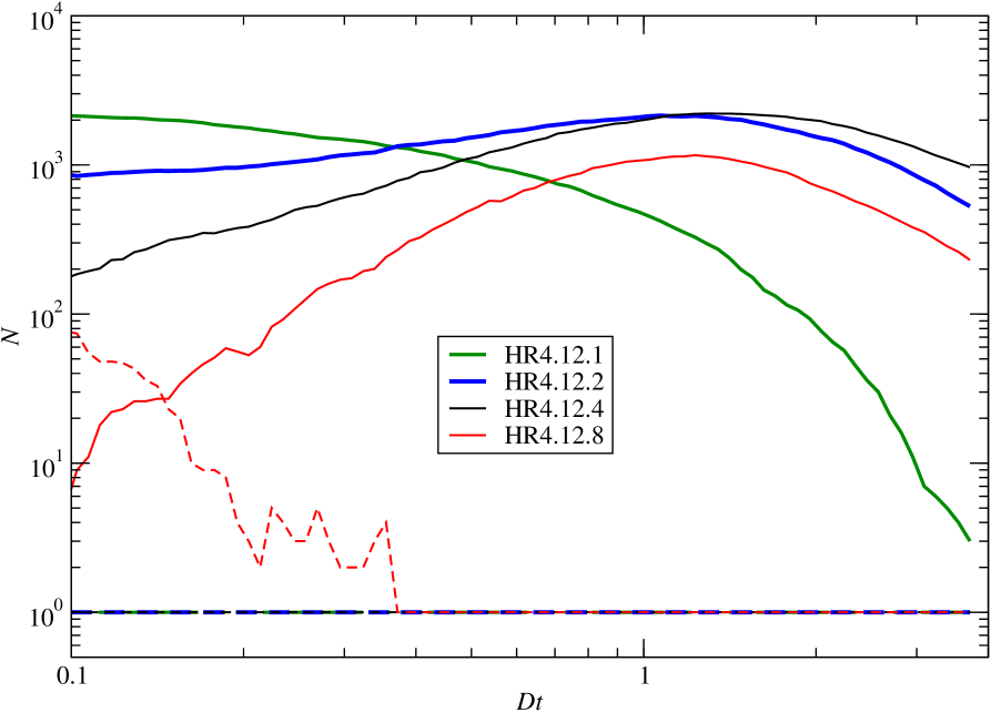
Figure 1: Percolation functions for unbiased L512.00 samples, biased L512.10 samples, SDSS.21 and HR4.12 samples, from top to bottom panels, respectively. Left panels are for filling factor functions, middle panels for cluster length functions, right panels for number functions. Functions for clusters are plotted with solid lines, and for voids with dashed lines.

3.1 Percolation analysis of distributions of matter and galaxies

The original percolation analysis was designed to measure the connectivity of percolating clusters (Stauffer, 1979), and was used by Zeldovich et al. (1982) and Melott et al. (1983) to investigate the connectivity of HDM and CDM models, respectively. The extended percolation method was designed by Einasto et al. (1986), Einasto & Saar (1987) and Einasto et al. (2018) to compare more general geometrical properties of models with observations. The density field is divided into high- and low-density regions, using a variable density threshold. Each element of the cosmic web belongs to a high- or low-density region, depending on the threshold. In this way the extended percolation analysis is a method to study various geometrical properties of the whole cosmic web over a large range of densities, and to compare models with observations.

Percolation functions describe how geometrical properties, such as sizes and volumes of largest clusters and voids, depend on the threshold used to divide the density field into high- and low-density regions. At high threshold density only the highest peaks (central regions of the largest cluster) are considered as over-density regions, and sizes and filling factors of largest clusters are small. As the density threshold decreases outer lower density regions of the clusters are included as parts of clusters, and lengths and filling factors of clusters increase. At certain density threshold the cluster merges with a neighbouring cluster, and the length and filling factor of the largest cluster increase. After several mergers the largest cluster spans the whole sample, i.e. it percolates (Liivamägi et al., 2012).

Fig. 1 presents percolation functions: filling factors of largest clusters and voids, $\mathcal{F}(D_{t})$, lengths of largest clusters and voids, ${L}(D_{t})$, and numbers of clusters and voids, $\mathcal{N}(D_{t})$, as functions of the threshold density, $D_{t}$, to divide the density field into over- and under-density regions. Functions are given for the full unbiased model L512.00, and for simulated and real galaxy samples, represented by the biased model L512.10, by the the luminosity limited sample SDSS.21, and by the halo mass limited model HR4.12. These simulated and real galaxy samples correspond approximately to $L_{\star}$ galaxies, see below.

The basic difference between the full model sample L512.00 and galaxy samples lies in the presence of the weak filamentary web in the L512.00 sample, which is absent in galaxy samples. Percolation functions describe this difference in various ways. In the full model L512.00 weak filaments and sheets fill the whole space, as seen in Fig. 14 below, which isolate small low-density regions (voids). This property of the web is characterised in the number function as follows: at small threshold densities the number of voids of the model L512.00 is high, see the upper right panel of Fig. 1. In contrast, at small threshold density high-density regions form one connected system — cluster, since low-density filaments join knots of the density field into one connected system. With increasing threshold density some filaments became fainter than the threshold density, the connected cluster splits to smaller units. Simultaneously there appear tunnels between small voids and voids merge. This leads to a rapid increase of the number of clusters, and a decrease of the number of voids with increasing $D_{t}$ (for smoothing length 1).

The presence of weak filaments and sheets in the full DM model L512.00 is expressed also in the filling factor and length functions. At small threshold densities the single high-density region (cluster) fills almost the whole sample volume, and the volume of the largest void is very small. Largest clusters percolate at threshold density $D_{t}=2-5$, largest voids percolate at $D_{t}=0.1-0.4$, depending on the smoothing scale.

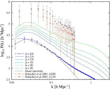
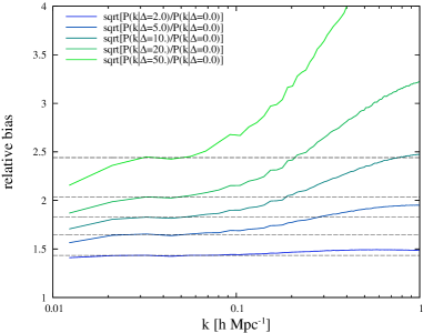
Figure 2: Left: Power spectra of particle density limited L512 model spectra. With open and filled symbols we show power spectra of X-ray flux-limited samples L050 and L120 of the REFLEX survey by Schuecker et al. (2001). For comparison the linear power spectrum is shown. Right: relative bias functions for power spectra of density limited L512 models.

In simulated and real galaxy samples low-density DM filaments and sheets are not present. This leads to important differences in percolation functions. First of all, voids are connected (percolated) at all threshold densities, thus the length of the largest void is equal to the size of the sample, and the number of voids is equal to 1. Only at very large smoothing kernels some additional voids appear at low $D_{t}$, created by excessively smoothed clusters. Filling factors of largest clusters are much lower than for full sample L512.00, and filling factors of largest voids are higher. The absence of connecting filaments between high-density knots of the web makes these knots isolated systems. For this reason the number of clusters at low threshold densities is rather large in all galaxy samples, in contrast to the sample L512.00. These small isolated clusters are seen in Fig. 14 in the model sample L512.10 and in the observed sample SDSS.21. The number of clusters, $\mathcal{N}(D_{t})$, is almost constant at $D_{t}\leq 2$ for all galaxy samples L512.10, SDSS.21 and HR4.12 for high-resolution density fields. Larger smoothing restores some filamentary connections between knots, thus the number of clusters decreases with decreasing $D_{t}$.

Notice that all percolation functions of simulated and real galaxy samples L512.10, SDSS.21 and HR4.12 are qualitatively very similar. Some minor quantitative differences are mainly due to the fact that the biased model selection parameter (particle density limit of the sample L512.10) is not exactly tuned for the best mutual agreement of percolation functions. This similarity is remarkable, since volumes and shapes of SDSS and L512 samples are very different, as mentioned above. The insensitivity of percolation functions to sample volumes, shapes and selection methods is an important property of the percolation method. This robustness of percolation functions has a simple explanation: percolation functions measure the growth of clusters (and voids) with decreasing threshold limit of the density field, $D_{t}$. The size, shape and volume of the largest over-density region (cluster) and largest under-density region (void) does not depend on the overall size (volume) and shape of the whole sample.

We conclude that the percolation analysis allows a reliable comparison on model and observed samples. The percolation analysis shows quantitatively the presence of large differences between the full DM dominated model L512.00 on the one side, and three versions of galaxy samples: L512.10, SDSS.21 and HR4.1 on the other side.

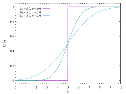
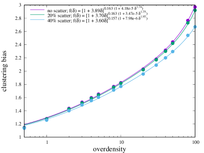
Figure 3: Left: The probability function $G(\delta)$ for L512.5 model with particle density limit $\delta_{0}=5$ and scatter of the particle density limit $\sigma=0,\leavevmode\nobreak\ 1,\leavevmode\nobreak\ 2$. Right: bias parameters $b$ as functions of the particle density limit, $\delta_{0}$, found from power spectra of biased models for particle density limits, $\delta_{0}$. Coloured filled circles show actually calculated bias parameters from spectra for three values of the scatter of the particle density limit, coloured curves show bias functions according to Eq. (3).

3.2 Recipes to select galaxy samples

Galaxy samples were selected for the percolation and power spectrum analyses using three recipes: halo mass limits, galaxy luminosity limits and particle local density limits. In principle we could use a simulated galaxy model, where halos are filled with galaxies using the halo occupation distribution (HOD), as done by Tinker & Conroy (2009) in the study of the void phenomenon. However, such synthetic galaxies are generated only inside DM halos, thus this model is actually a variant of the HR4 model. Comparison of galaxy and matter samples was made using respective density fields. The difference in the calculation of respective density fields lies in the use of spatial coordinates. In halo mass limited samples only positions of halo centres were used. Large halos host many galaxies and have dimensions exceeding the resolution scale of density fields, 1 $h^{-1}$ Mpc. Thus density fields, calculated from halo data, are more rough, what is seen also in high-resolution density field maps. If data on locations of individual galaxies are used, as in the case of SDSS samples, we get a more smooth density field. When positions of all individual particles are used, as in the case of L512 model based density fields, we get an even more smooth density field. However, differences in density fields are small (see Fig. 14), and have little influence to percolation functions and the distribution of densities. For this reason percolation functions and density distributions of real and simulated galaxies are qualitatively very similar, as seen in Figs. 1, 5, 6, and 7.

4 Power spectra and bias parameters of models

In this Section we calculate power spectra of biased L512 model samples. We investigate the influence of fuzzy particle density limit. Our goal is to find the bias as a function of the particle density limit $\delta_{0}$, used in the selection of biased model samples.

4.1 Power spectra of biased L512 models

We calculated power spectra of full L512.00 model with all DM particles included, $P_{m}=\Delta_{m}^{2}(k)$, and for biased model L512.i samples (clustered particle samples), $P_{C}(k,\delta_{0})=\Delta_{C}^{2}(k,\delta_{0})$, using particle density limits, $\delta_{0}$, according to Table 1. We applied standard procedures, used to calculate power spectra of numerical simulations (Eisenstein & Hu, 1999). Power spectra for the full model L512.00 and for biased models L512.i, are shown in left panels of Fig. 2. The blue solid line with error ticks is for the spectrum of the model with all matter, L512.00 (particle density limit $\delta_{0}=0$). Black dashed line shows the linear power spectrum for this model. Thin coloured lines are for power spectra, calculated for biased L512.i models according to Table 1. Symbols with error bars are power spectra of flux-limited X-ray selected clusters of galaxies, samples L050 and L120, according to Schuecker et al. (2001).

Right panel of Fig. 2 shows relative bias functions $b_{C}(k,\delta_{0})=\sqrt{P_{C}(k,\delta_{0})/P_{m}(k)}$. Bias functions depends on the wavenumber $k$. They have a plateau around $k\approx 0.03$ $h$ Mpc^-1, similar to the plateau found by Percival et al. (2001). We used the plateau at $k\approx 0.03$ $h$ Mpc^-1 to find bias parameters for model samples as a function of particle density limits. Results are seen as dark circles in the upper curve on the right panel of Fig. 3.

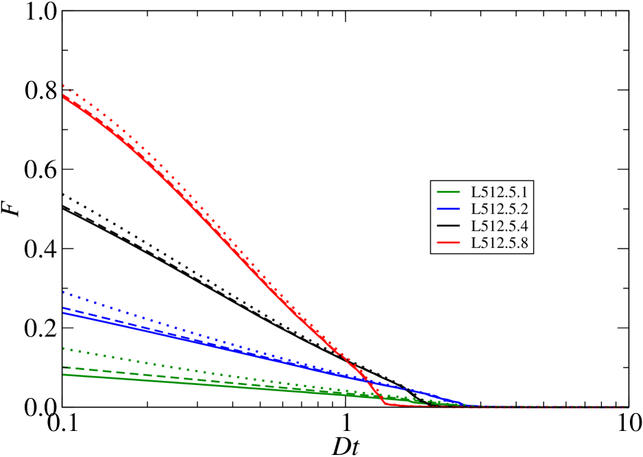
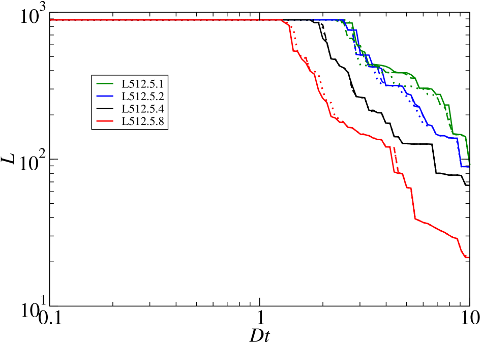
Figure 4: Percolation functions using fuzzy particle density limits of the model L512.5 with $\delta_{0}=5$. Left: filling factor functions, right: length functions of largest superclusters. Solid lines are for functions with fuzziness dispersion $\sigma=0$, i.e. sharp particle density limit, dashed lines are for dispersion $\sigma=1$ and dotted lines for $\sigma=2$.

4.2 Influence of a fuzzy particle density limit

The use of the local density $\delta_{0}$ as the only parameter to determine the fate of particles in the web is a simplification. Actually particles of slightly variable densities can end up in halo-type density enhancements, which can be considered as model equivalents to real galaxies. For this reason the density limit to divide particles into high- and low-density populations is fuzzy.

To find the influence of a fuzzy particle density limit we made the power spectrum and percolation function analyses for the L512 model, using a series of particle local density limits. We selected particles for this model as follows: particle with local densities $x\leq x_{min}$ are excluded, particles with densities $x$ within limits $x_{min}\dots x_{max}$ are included with a probability $G(x)$, which depends on the location within the window, and particles with densities $x>x_{max}$ are all included. Here we use the designation $x=D(\mathbf{x})/D_{m}$, where $D(\mathbf{x})$ is the density at location $\mathbf{x}$, and $D_{m}$ is the mean density. Limits $x_{min}$ and $x_{max}$ are determined by the choice of the fuzziness distribution function $p(x)$. The probability function $G(x)$ to include particles to the clustered population was calculated applying the standard procedure:

$$G(x)=\int_{0}^{x}p(x)dx.$$ (1)

For the fuzziness distribution function we used the normal distribution

$$p(x)dx=\frac{1}{\sigma\sqrt{2\pi}}\exp[-\frac{(x-x_{0})^{2}}{2\sigma^{2}}]dx,$$ (2)

where $x_{0}=\delta_{0}$ is the location of the sharp limit, and the dispersion of the particle density limit $\sigma$ depends on the location of the limit, $\sigma=f\times\delta_{0}$; $f$ is the fuzziness parameter.

Power spectra were calculated for a series of particle density limits, $\delta_{0}$, using fuzziness parameter values $f=0.1,\leavevmode\nobreak\ 0.2,\leavevmode\nobreak\ 04$. The limit $f=0$ corresponds to a sharp particle density limit at $\delta_{0}$. Probability distributions $G(\delta)$ are shown in the left panel of Fig. 3 for the particle density limit $\delta_{0}=5$. It should be noticed that the form of the function $G(\delta)$ is the same for all particle density limit values, since the dispersion $\sigma$ is proportional to the density limit, $\delta_{0}$. Using power spectra we calculated the clustering bias parameter $b$, shown by coloured filled symbols in the right panel of Fig. 3.

The bias parameter as function of the particle density limit can be approximated as follows:

$$b(\delta_{0})=(1+a\leavevmode\nobreak\ \delta_{0})^{c(1+d\leavevmode\nobreak\ \delta_{0}^{n})}.$$ (3)

This approximation gives a good fit of biased L512 models within particle density limits $0.5\leq\delta_{0}\leq 100$, see coloured lines in Fig. 3. Parameters [a, c, d, n] depend on the fuzziness parameter $f$, used in calculations of power spectra. For $f=0$ and $f=0.1$ parameters have values [a, c, d, n] = [3.89, 0.163, 4.18E-5, 1.74], for $f=0.2$ we get [a, c, d, n] = [3.70, 0.163, 3.47E-5, 1.75], and for $f=0.4$ we have [a, c, d, n] = [3.60, 0.157, 7.98E-6, 1.95].

We calculated density fields and made the percolation analysis for the model L512.5, using the particle density limit $\delta_{0}=5$, the scatter of particle density limit $\sigma=1,\leavevmode\nobreak\ 2$, and applying smoothing kernels $R_{B}=1,\leavevmode\nobreak\ 2,\leavevmode\nobreak\ 4,\leavevmode\nobreak\ 8$ $h^{-1}$ Mpc. Percolation functions $F(D_{t})$ and $L(D_{t})$ are shown in Fig. 4. Solid lines are for functions using sharp particle density limits with $\sigma=0$, dashed lines using particle density limit scatter $\sigma=1$, and dotted lines with scatter $\sigma=2$, which correspond to fuziness parameter values $f=0.0,\leavevmode\nobreak\ 0.2,\leavevmode\nobreak\ 0.4$, respectively. Our results indicate that the scatter $\sigma=1$ yields percolation functions, almost identical to percolation functions with a sharp particle density limit, $\sigma=0$. Even the very large scatter $\sigma=2$ causes very small changes to percolation functions. These calculations showed that power spectra and percolation functions for fuzzy particle density limit are close to results obtained with a sharp limit. Near the low particle density limit $\delta_{0}$ the fraction of matter in high-density regions, $F_{C}$, determines the effective biasing factor, as shown already by Einasto et al. (1999). Thus we consider the particle density limit $\delta_{0}$ as an effective limit.

The bias function,

$$b_{C}(\delta_{0})=\sqrt{P_{C}(0.03,\delta_{0})/P_{m}(0.03)},$$ (4)

is given in Table 1 and in Fig. 3. It was calculated using the plateau at $k=0.03$ Mpc^-1 and applying a smoothed value according to Eq. (3). The bias function yields an one-to-one relationship between the bias parameter $b$ and the particle selection parameter $\delta_{0}$ of biased models. The bias function depends on the cosmological parameters of the model, but only weakly, since we use ratios of power spectra of the same model. It depends also on the particle selection method. The fuzziness analysis shows that the selection method is rather robust.

5 Percolation analysis of simulated and real galaxy fields

In this Section we continue the extended percolation analysis of observed and simulated clusters. We compare percolation functions for different limiting parameters (luminosities of galaxies, particle density limits, masses of halos), and for different samples — observed vs. simulated samples. Our goal is to find density limits $\delta_{0}$ of biased models, which correspond to luminosity limited SDSS samples, and mass limited HR4 samples.

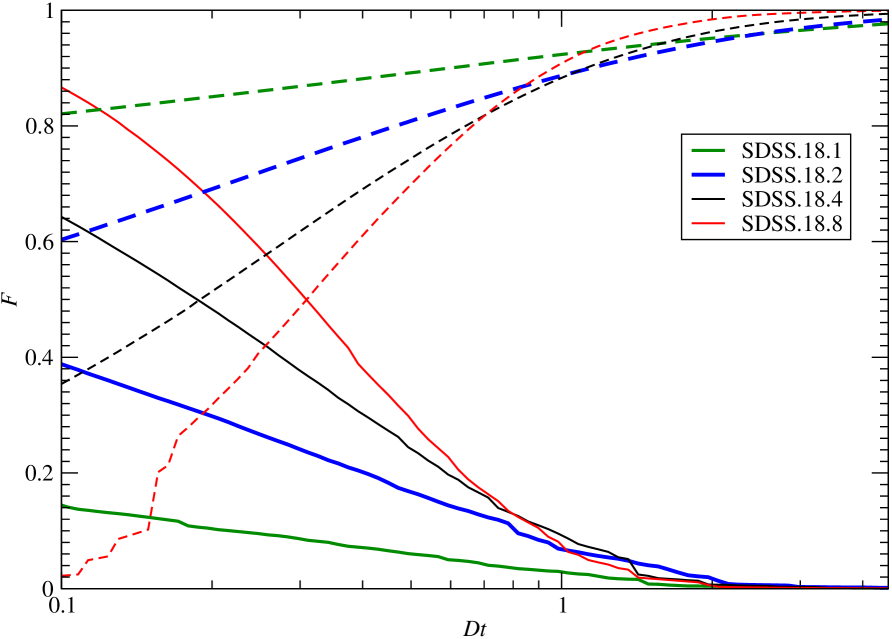
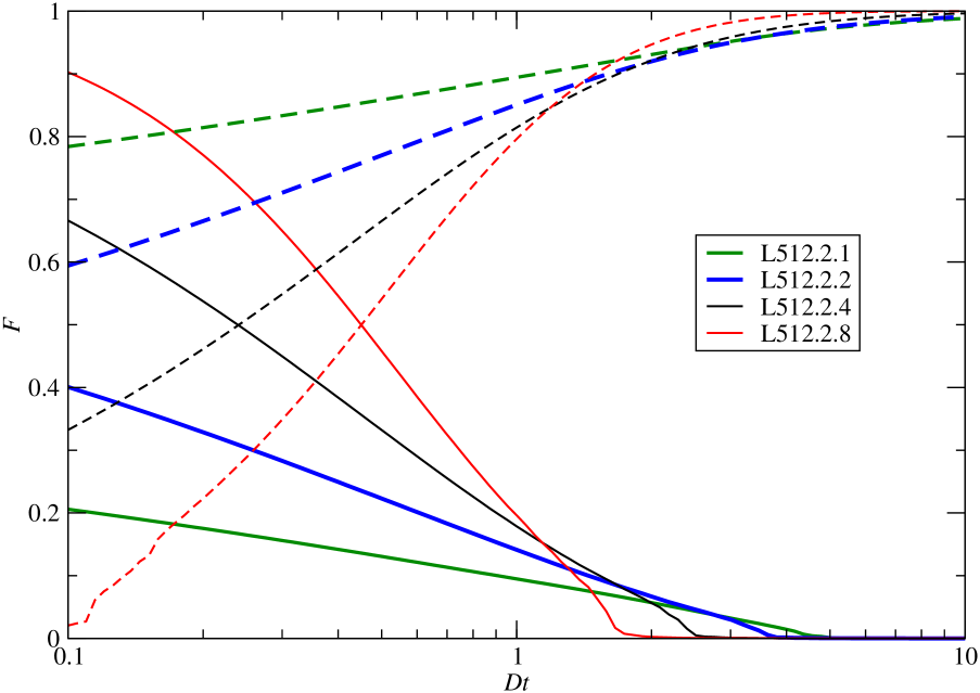
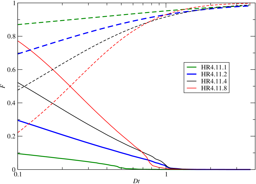
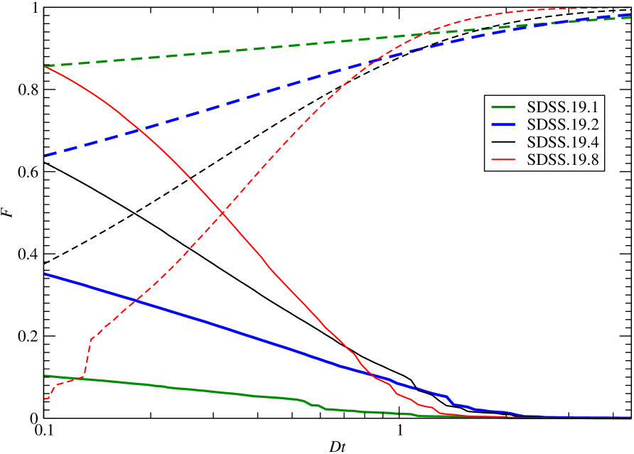
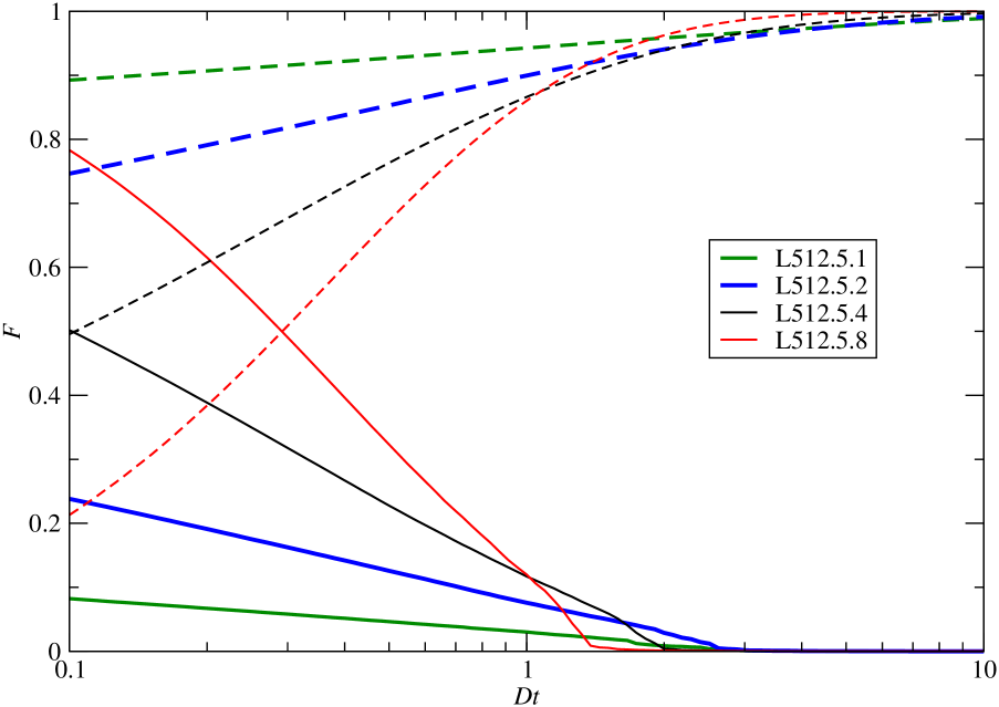
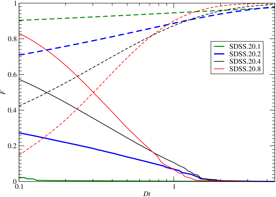
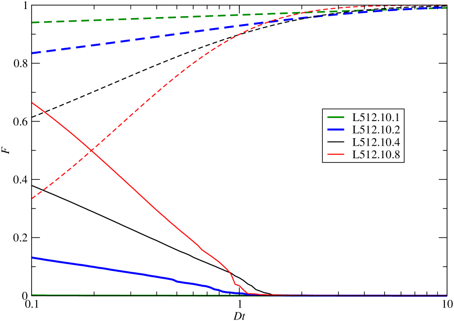
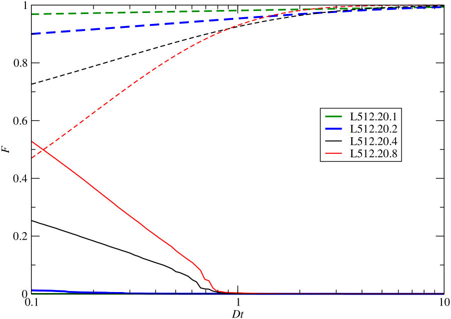
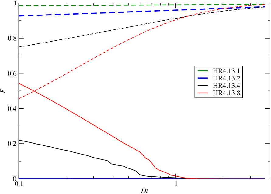
Figure 5: Filling factor functions of largest clusters and voids, $\mathcal{F}(D_{t})=V_{\mathrm{max}}/V_{0}$, as functions of the threshold density, $D_{t}$. Left panels: luminosity limited SDSS samples, middle panels particle density limited (biased) L512 model samples, right panels: HR4 model samples. Left panels from top to bottom are for luminosity limits $M_{r}-5\log h=-18.0,\leavevmode\nobreak\ -19.0,\leavevmode\nobreak\ -20,0,\leavevmode\nobreak\ -21.0$; middle panels from top to bottom are for samples with particle density limit $\delta_{0}=2,\leavevmode\nobreak\ 5,\leavevmode\nobreak\ 10,\leavevmode\nobreak\ 20$; right panels from top to bottom are for halo mass limited samples HR4.11, HR4.12, HR4.123, HR4.13. Functions for clusters are plotted with solid lines, and for voids with dashed lines.

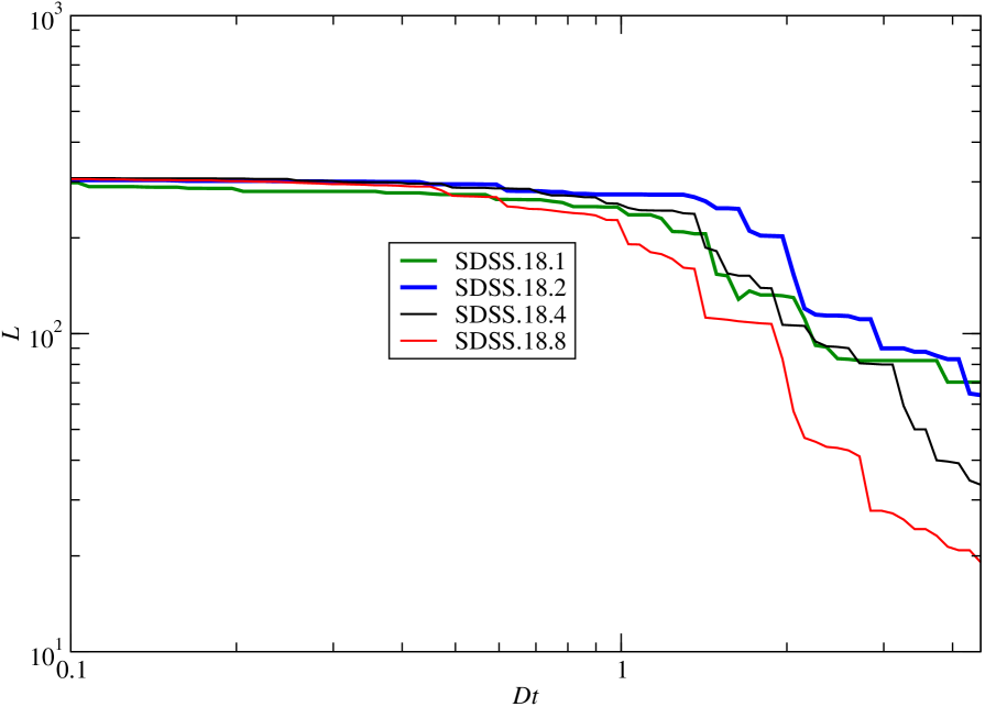
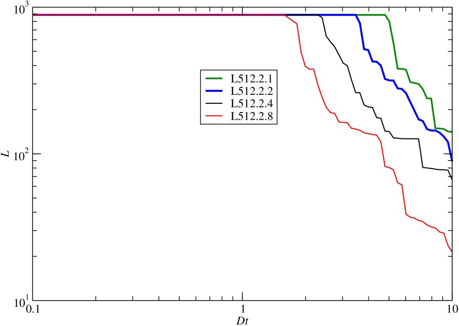
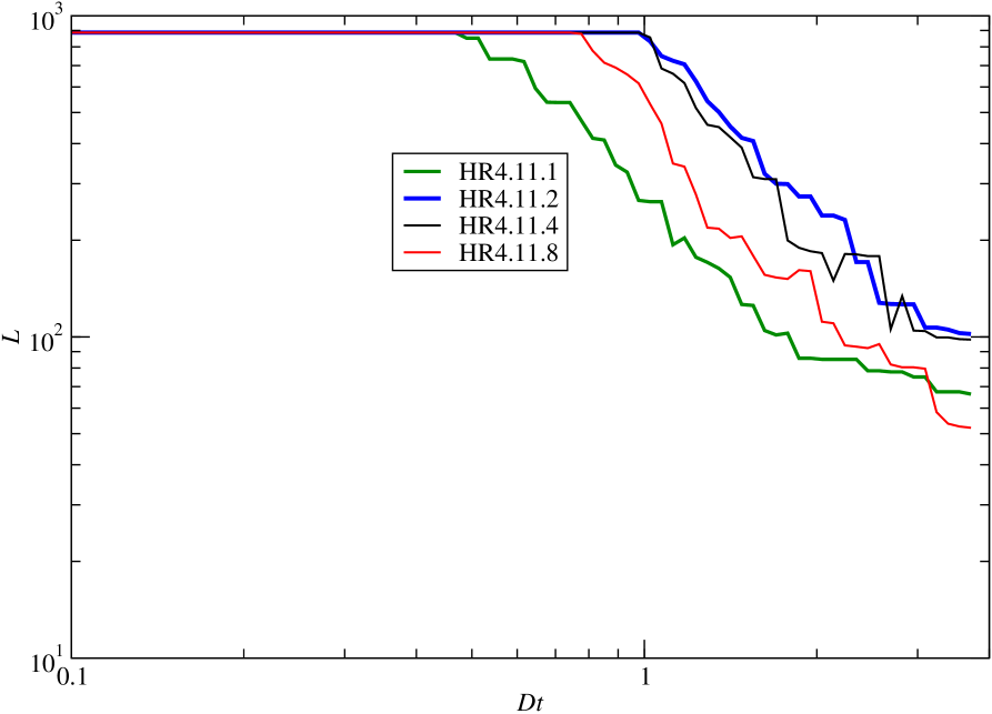
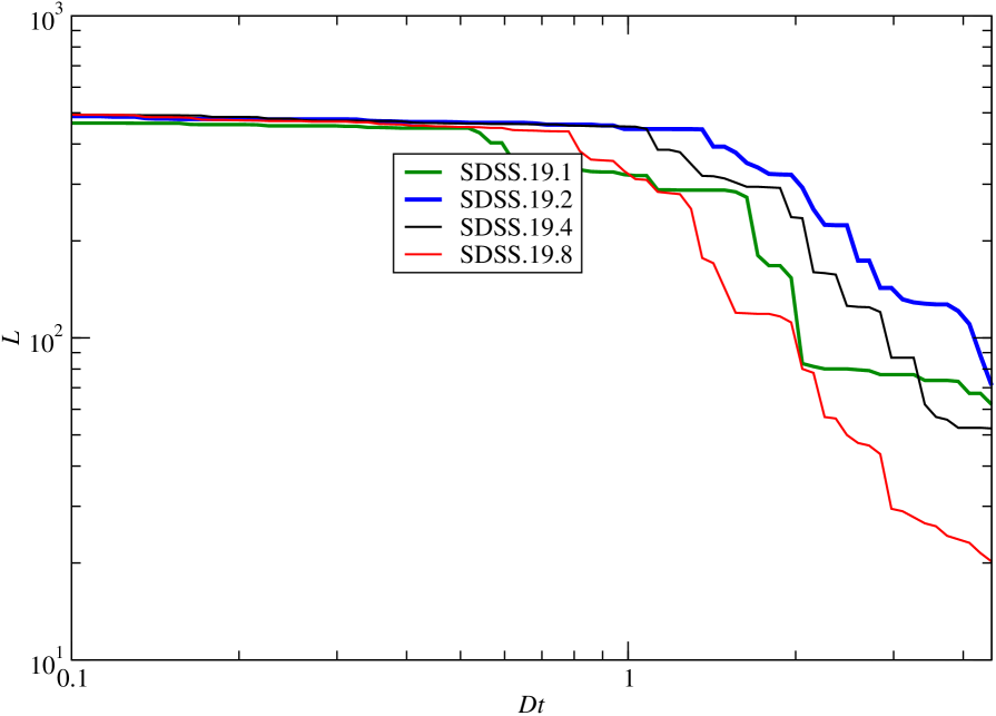
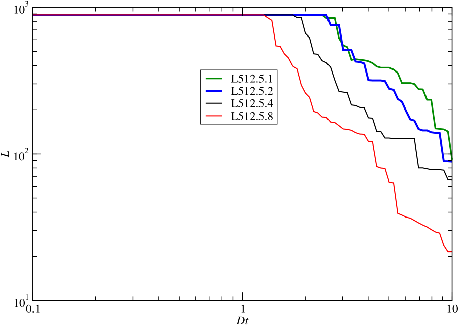
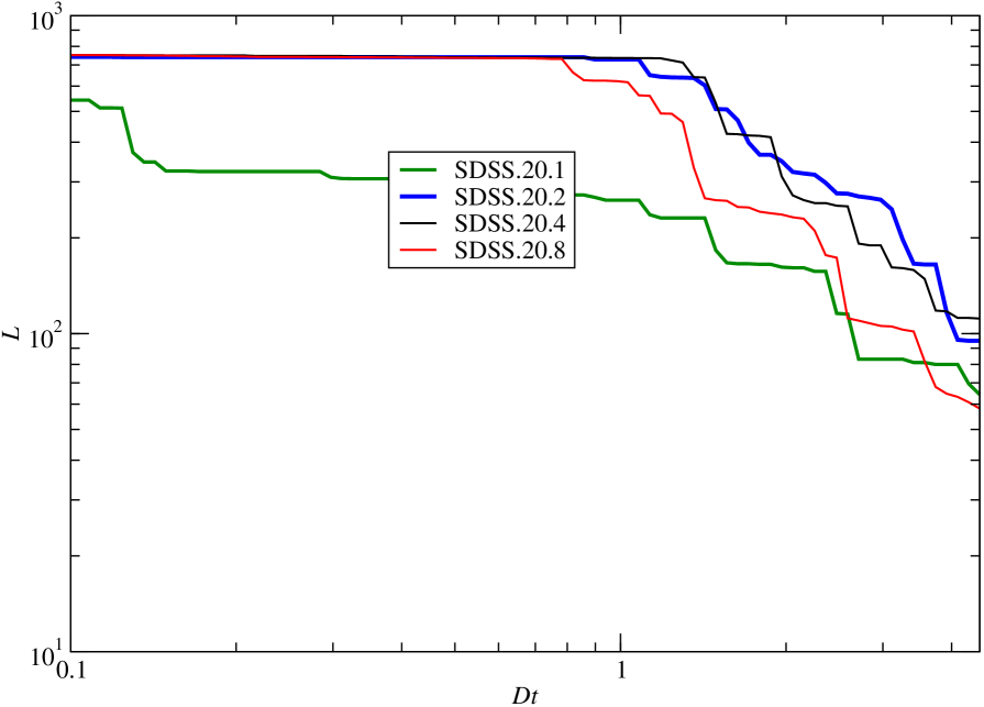
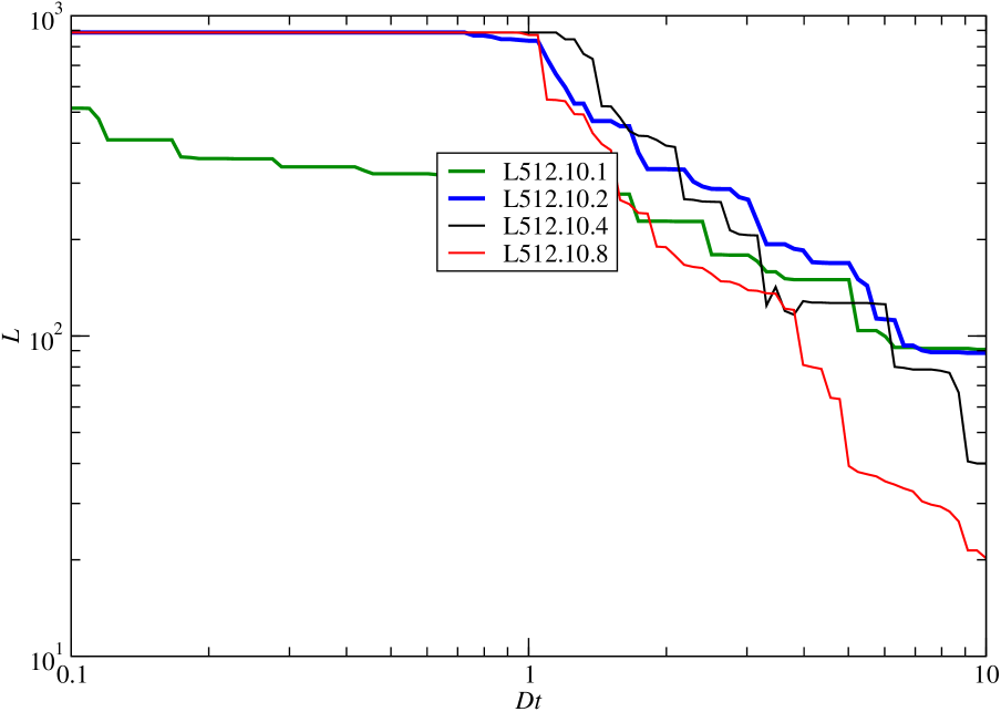
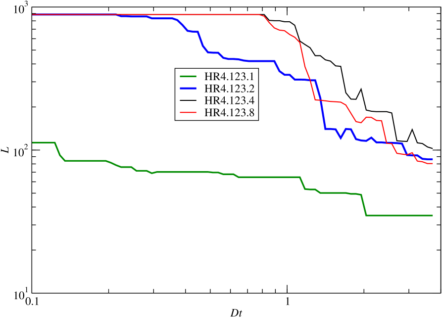
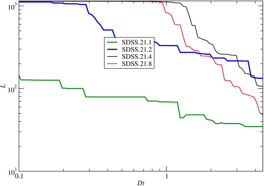
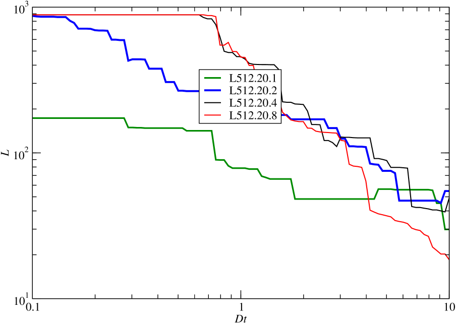
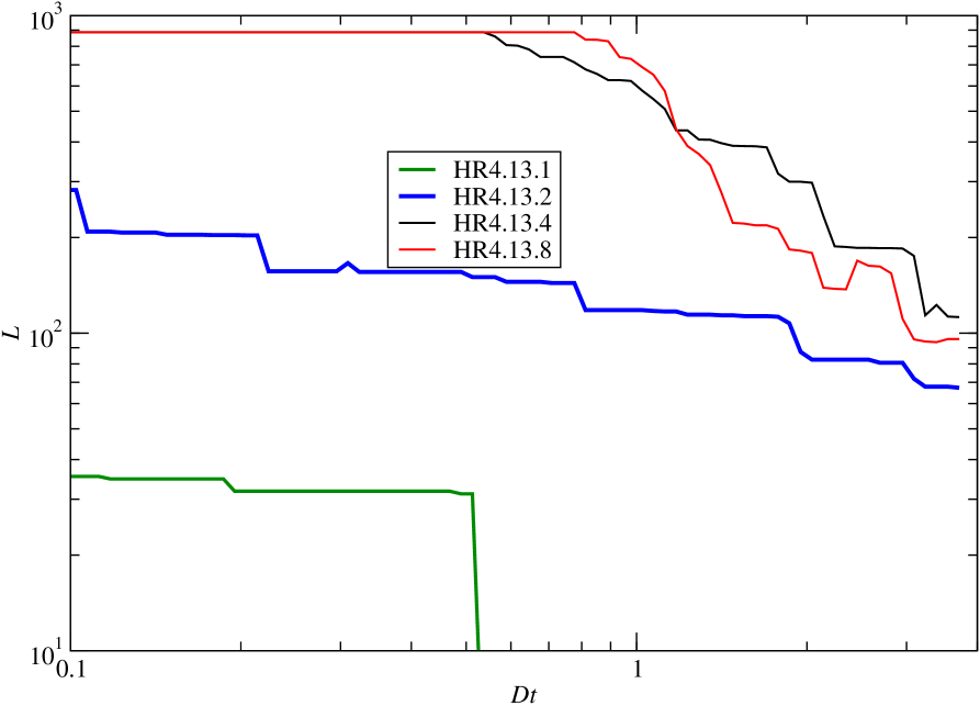
Figure 6: Length functions of largest clusters, ${L}(D_{t})=L_{\mathrm{max}}$ in $h^{-1}$ Mpc. Panels and lines as in Fig. 5.

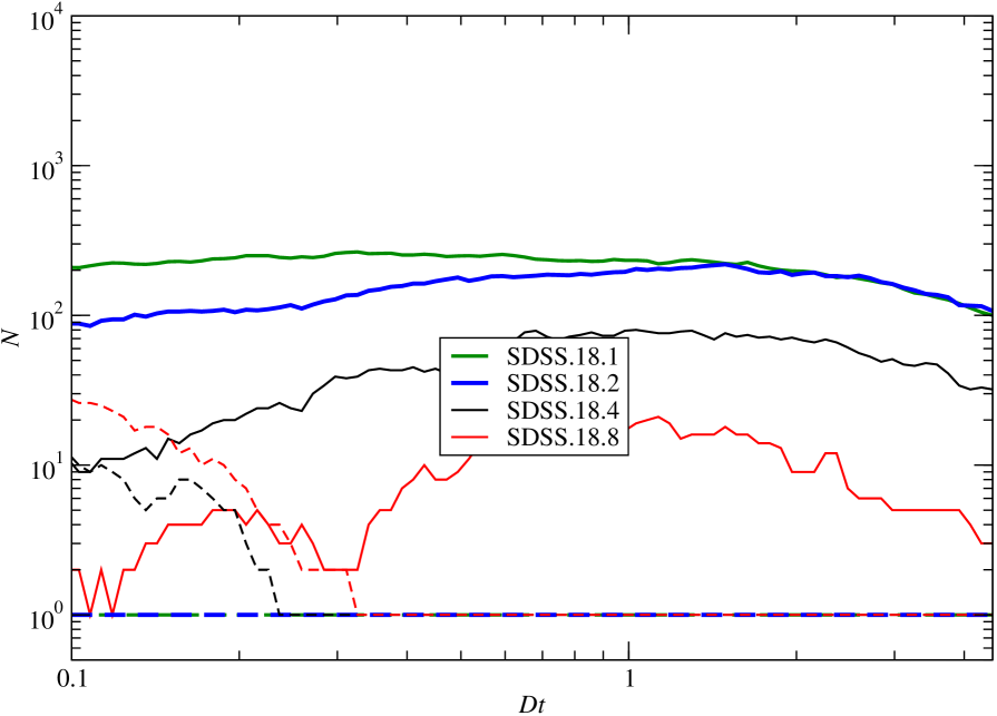
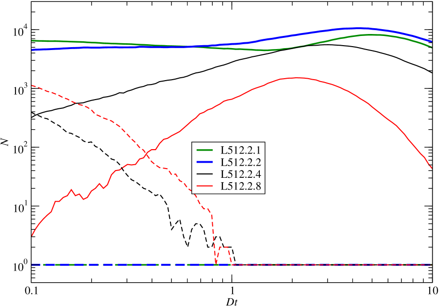
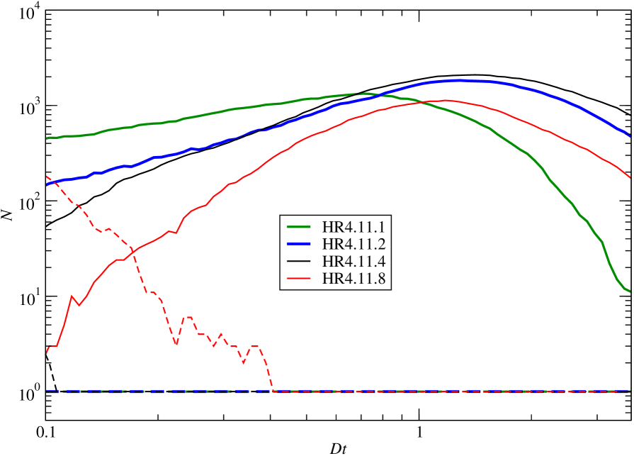
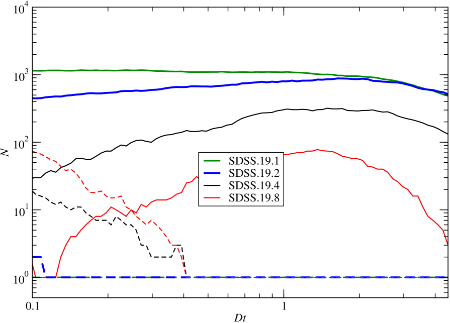
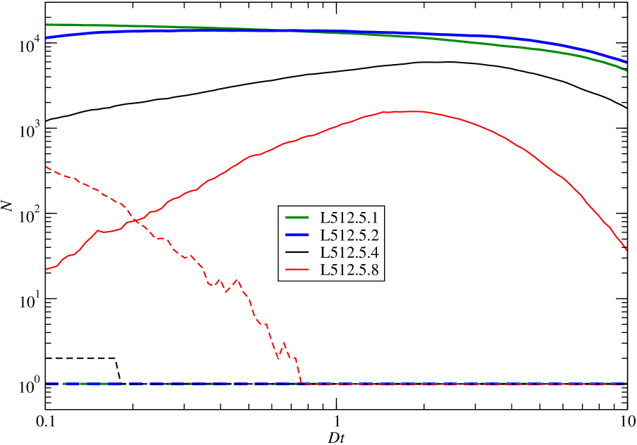
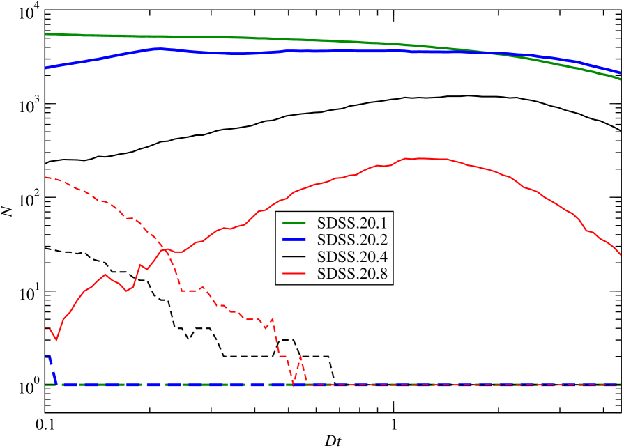
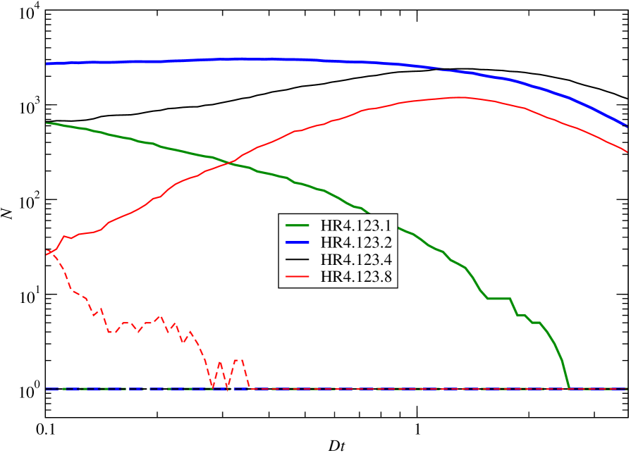
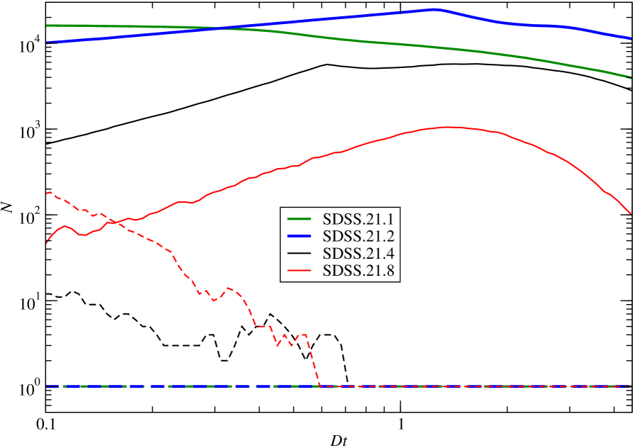
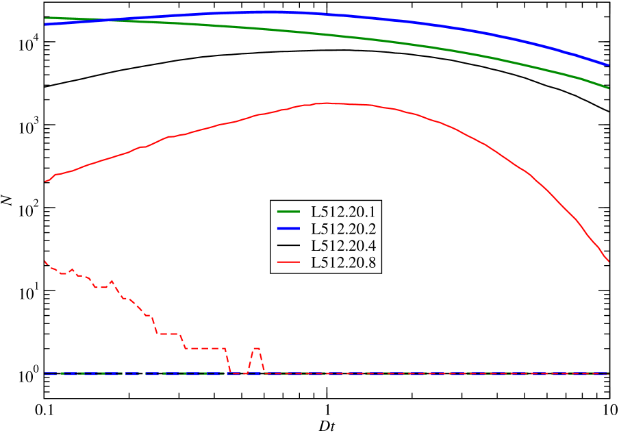
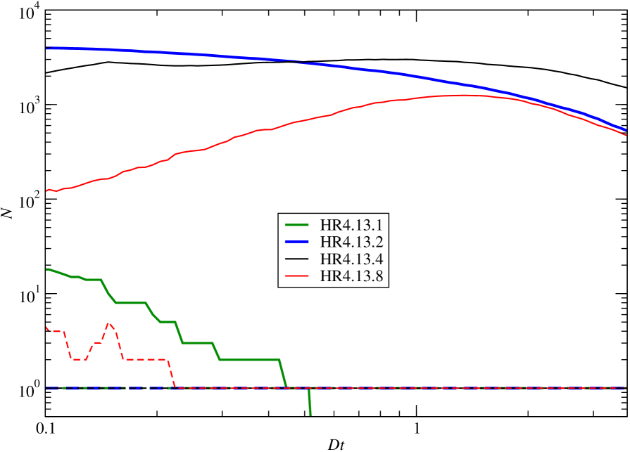
Figure 7: Number of clusters and voids, $\mathcal{N}(D_{t})$. Number functions are calculated with small system exclusion limit $N_{\mathrm{lim}}=50$ (L512 and SDSS samples); and with $N_{\mathrm{lim}}=500$ (HR4 samples). Lines as in Fig. 5.

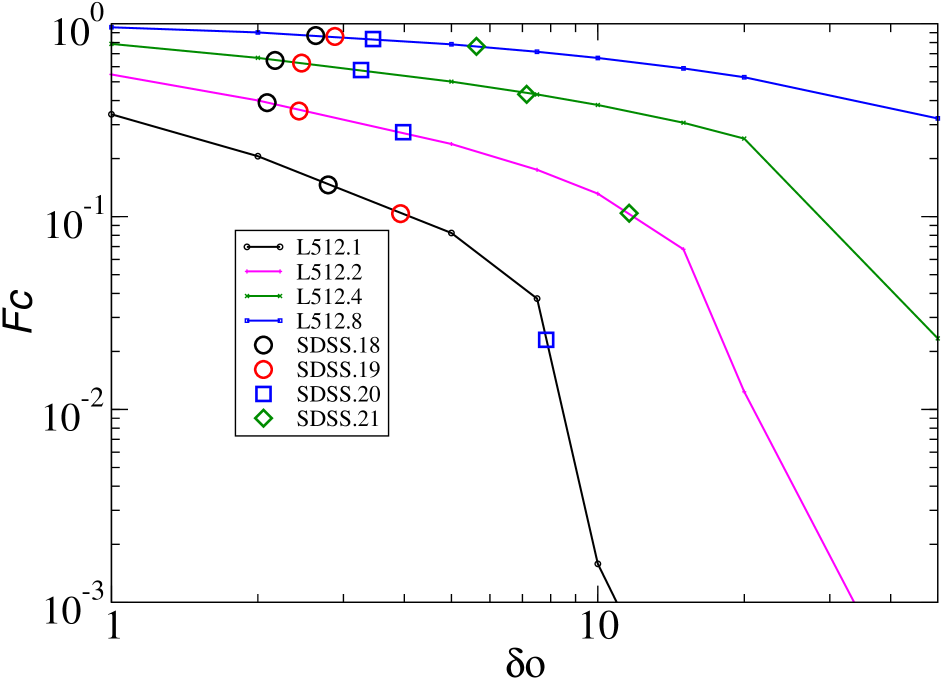
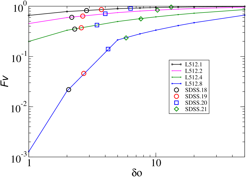
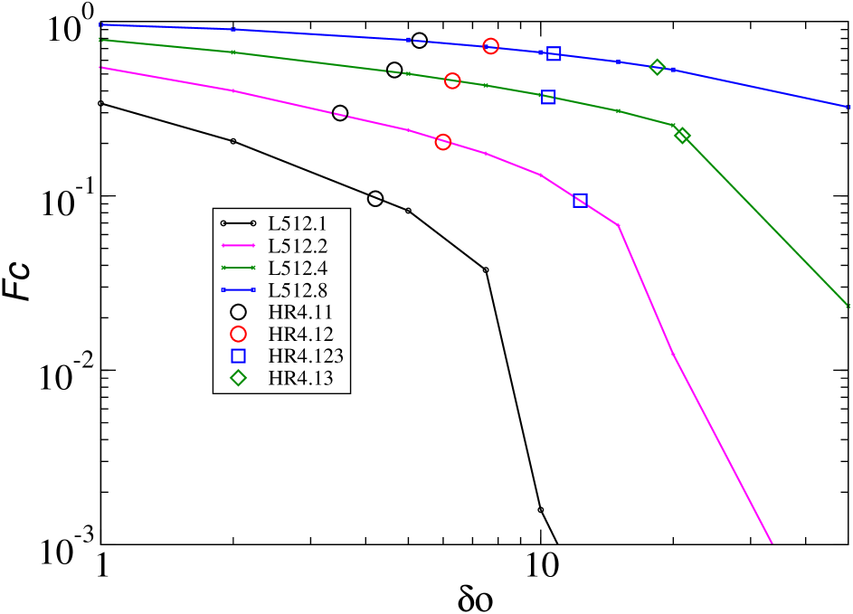
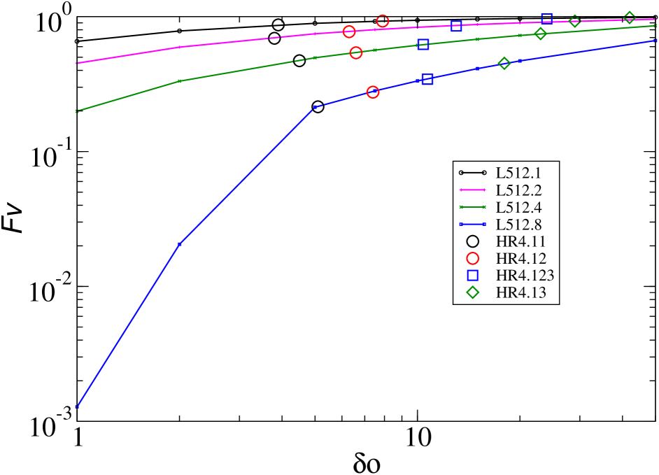
Figure 8: Filling factor test function of clusters $F_{C}(\delta_{0})$ and voids $F_{V}(\delta_{0})$. Solid lines show test functions of L512 models for four smoothing scales, $R_{B}=1,\leavevmode\nobreak\ 2,\leavevmode\nobreak\ 4,\leavevmode\nobreak\ 8$ $h^{-1}$ Mpc. Left panels are for cluster filling factors, right panels for void filling factors. Upper panels show by symbols filling factors of SDSS samples, lower panels filling factors of HR4 samples.

5.1 Percolation properties of observed and model samples

Percolation properties depend on the smoothing kernel size, since smoothing makes clusters and connecting filaments larger and helps clusters to percolate. We calculated density fields of observed and model samples, expressing densities in units of the mean density of particular samples. The L512 model sample includes all particles of the model, the HR4 model sample includes all halos, containing at least 30 particles, the SDSS samples includes all galaxies within the apparent r magnitude interval $12.5\leq m_{r}\leq 17.77$. Using density fields with these normalisations we calculated all percolation functions.

The comparison of percolation functions of observed SDSS samples and HR4 model samples with percolation functions of L512 model samples showed that percolation functions of SDSS and HR4 samples are shifted relative to L512 model samples towards higher threshold densities. This is a well-known effect. All densities are expressed in mean density units. In model samples the mean density includes, in addition to clustered matter, also DM in low-density regions, where there are no galaxies, or galaxies are fainter than the magnitude limit of the observational SDSS survey. In calculations of the mean density of observed SDSS samples and HR4 model samples unclustered and low-density DM is not included. This means that in the calculation of densities in mean density units densities are divided to smaller numbers, which increases density values of SDSS and HR4 samples.

The total number and mass of particles of HR4 model samples is known, thus it is easy to calculate the density normalisation factor, which brings density fields to the level, corresponding to all particles. We found that the fraction of particles in our HR4 samples is $f=0.37156$. To bring HR4 density fields to the same normalisation as L512 density fields, we multiplied all threshold densities by the factor $f$. Corrected density thresholds can be used as arguments in percolation functions. Since we plot percolation functions using as argument $\log(D_{t})$, the shape of functions does not depend on the normalisation factor, and we can use the same functions as in our preliminary analysis, only the argument is shifted.

The comparison of percolation functions of SDSS and HR4 samples shows that the SDSS sample contains galaxies which correspond to less massive halos than the HR4 sample. For this reason the correction factor $f$ for SDSS samples must be closer to unity. The exact value of this factor is difficult to calculate. Our analysis of percolation functions and respective parameters using various density normalisation factors shows that final results depend on the exact value of the factor $f$ only rather modestly. We accepted for SDSS samples the factor $f=0.45$.

Using corrected density normalisations we show in Fig. 5 filling factor functions of largest clusters and voids, $\mathcal{F}(D_{t})=V_{\mathrm{max}}/V_{0}$, in Fig. 6 length functions — lengths of largest clusters, ${L}(D_{t})=L_{\mathrm{max}}$ in $h^{-1}$ Mpc, and in Fig. 7 numbers functions $\mathcal{F}(D_{t})$. Length functions of voids are not defined since voids percolate at all threshold densities. Left panels in Figures are for luminosity limited SDSS samples, middle panels for particle density limited L512 samples, using particles density limits $\delta_{0}=2,\leavevmode\nobreak\ 5,\leavevmode\nobreak\ 10,\leavevmode\nobreak\ 20$, and right panels for halo mass limited HR4 model samples. In functions as argument we use the threshold density, $D_{t}$, corrected for sample mean density normalisation. Solid lines in Figures are for clusters, dashed lines for voids; colours mark different smoothing lengths.

Figs. 5, 6 and 7 show that percolation functions of observed and model samples have surprisingly similar shapes, and depend in a simple and regular way on sample parameters. The difference between filling factor functions of observed and model samples is the largest at lowest threshold density, $D_{t}=0.1$. Thus we shall use filling factor function values at threshold density, $D_{t}=0.1$ as test parameters to compare samples in a quantitative manner. The behaviour of length functions is more complicated and is discussed later.

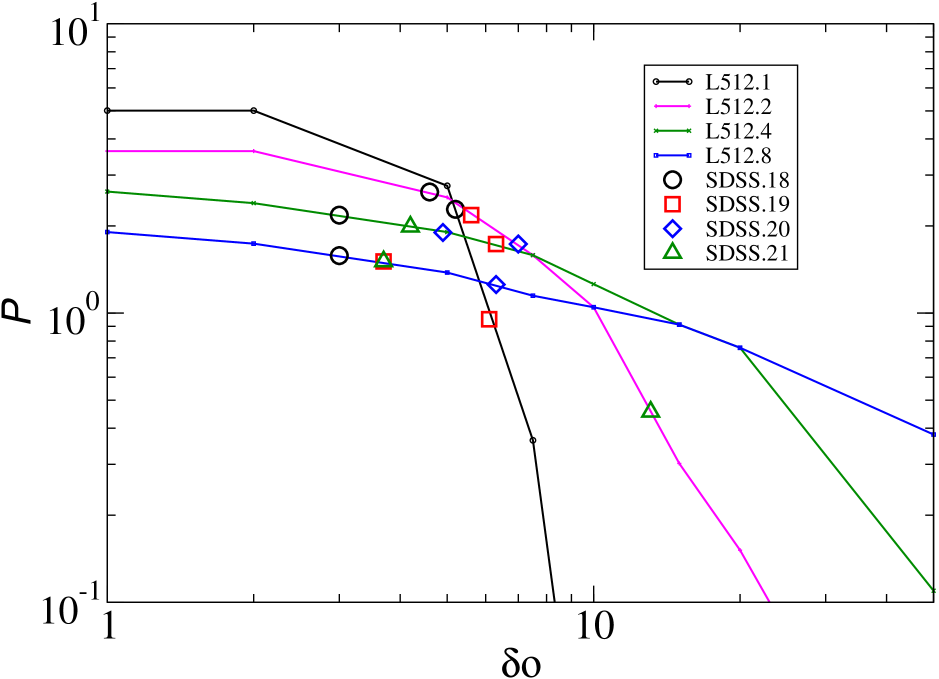
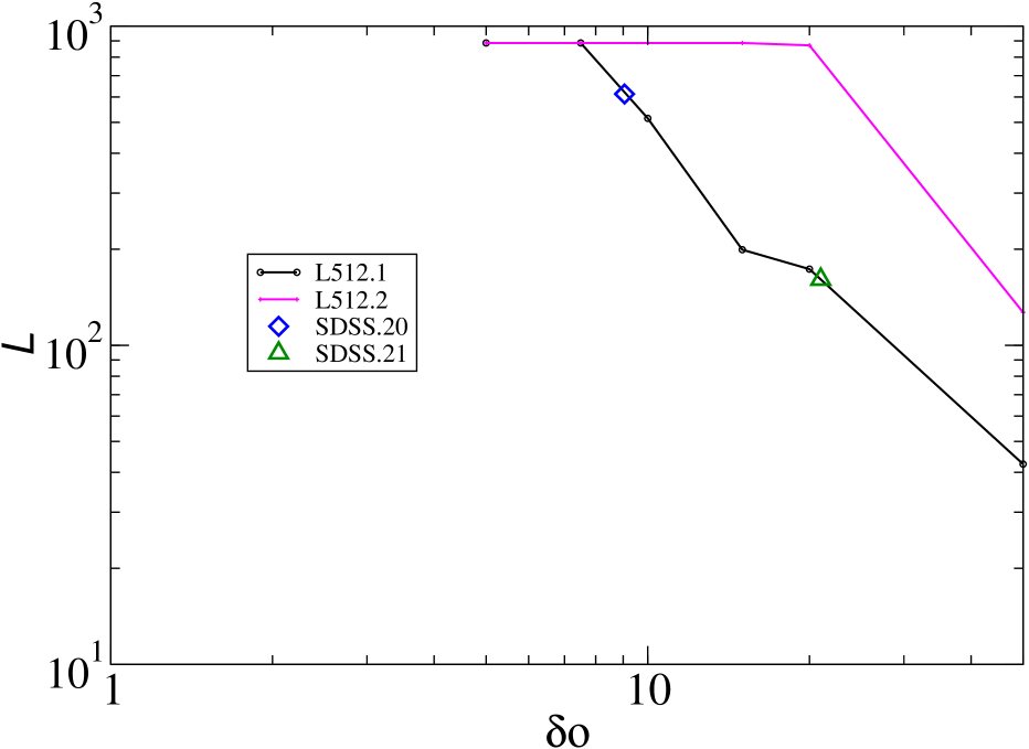
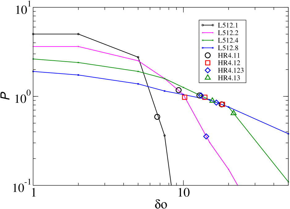
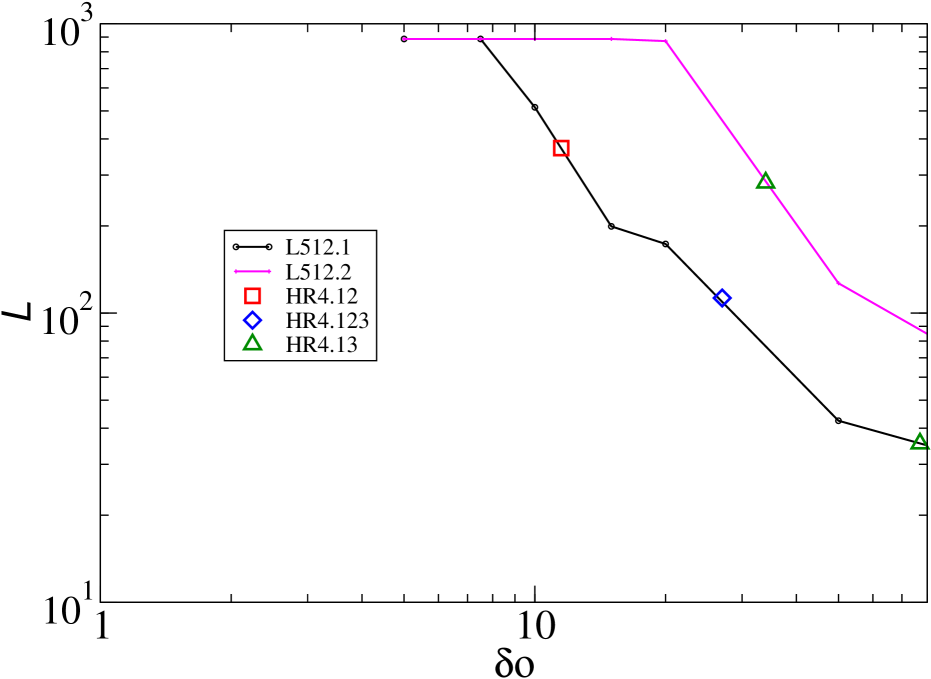
Figure 9: Left panels shows the cluster percolation threshold test, righ panels show the cluster length test for high-luminosity (mass) samples. Upper panels are for SDSS samples, lower panels for HR4 samples;. Solid lines show cluster length test functions of L512 models for various smoothing scales. Coloured symbols show SDSS samples of various luminosity and HR4 samples of various halo mass limits.

5.2 Filling factor test of clusters and voids

The cluster filling factor test parameter is defined as $F_{C}=\mathcal{F}_{C}(0.1)$, and the void filling factor test parameter as $F_{V}=\mathcal{F}_{V}(0.1)$. Each sample with a different particle density limit $\delta_{0}$ and smoothing kernel size $R_{B}$ yields a value for $F_{C}$ and $F_{V}$. We calculated these parameters of the L512 model for a range of particle density limits $\delta_{0}$, and define filling factor test functions as follows: $F_{C}(\delta_{0})$ and $F_{V}(\delta_{0})$. Our goal is to find particle density limits $\delta_{0}$ of L512 models which correspond to galaxy luminosity limits of SDSS samples and halo mass limits of HR4 samples. We shall use the following strategy: we plot filling factor test functions $F_{C}(\delta_{0})$ and $F_{V}(\delta_{0})$ of biased models L512, separately for smoothing kernels $R_{B}=1,\leavevmode\nobreak\ 2,\leavevmode\nobreak\ 4,\leavevmode\nobreak\ 8$ $h^{-1}$ Mpc. Results are shown in Fig. 8. Solid lines are for biased L512 models, different colours mark functions calculated using smoothing scales $R_{B}=1,\leavevmode\nobreak\ 2,\leavevmode\nobreak\ 4,\leavevmode\nobreak\ 8$ $h^{-1}$ Mpc. Left panels are for cluster filling factors, and right panels for void filling factors. Filling factors of SDSS and HR4 samples of various luminosity limits are known, and it is easy to interpolate, at which particle density limits $\delta_{0}$ filling factors of SDSS (HR4) samples are equal to filling factors of biased L512 samples. This comparison was made separately for each smoothing kernel value, $R_{B}$, and for filling factors of clusters and voids. We tried several interpolation schemes, and found that good results are obtained by linear interpolation along the $\log\delta_{0}$ axis.

Table 4: Particle density limit and bias parameters of SDSS and HR4 samples.

Sample	$(\delta_{0})_{F}$	$(\delta_{0})_{L}$	$(\delta_{0})_{Ls}$	$b_{F}$	$b_{L}$	$b_{Ls}$
(1)	(2)	(3)	(4)	(5)	(6)	(7)
SDSS.18	$2.5\pm 0.4$	$4.9\pm 1.0$	$5\pm 2$	$1.47\pm 0.03$	$1.63\pm 0.05$	$1.64\pm 0.11$
SDSS.19	$3.2\pm 0.8$	$5.9\pm 1.5$	$6\pm 2$	$1.53\pm 0.06$	$1.68\pm 0.07$	$1.68\pm 0.09$
SDSS.20	$5.5\pm 1.9$	$8.0\pm 2.0$	$10\pm 3$	$1.66\pm 0.09$	$1.76\pm 0.07$	$1.83\pm 0.09$
SDSS.21	$13.0\pm 2.9$	$17\pm 4$	$20\pm 5$	$1.91\pm 0.07$	$1.99\pm 0.08$	$2.05\pm 0.09$
HR4.11	$3.8\pm 0.4$	$8.0\pm 1.5$	$6\pm 2$	$1.57\pm 0.02$	$1.76\pm 0.05$	$1.68\pm 0.09$
HR4.12	$8.0\pm 2.6$	$10.8\pm 2.0$	$10\pm 4$	$1.76\pm 0.09$	$1.85\pm 0.06$	$1.83\pm 0.12$
HR4.123	$21\pm 10$	$21\pm 5$	$20\pm 5$	$2.06\pm 0.18$	$2.07\pm 0.09$	$2.05\pm 0.09$
HR4.13	$42\pm 13$	$56\pm 8$	$40\pm 10$	$2.35\pm 0.16$	$2.51\pm 0.09$	$2.33\pm 0.12$

Using this interpolation scheme we found for each SDSS luminosity limit (HR4 sample halo mass limit) particle density limits $\delta_{0}$ of biased L512 samples, which correspond to these SDSS (HR4) samples, separately for clusters and voids, and for different smoothing kernel length, $R_{B}$. Fig. 8 show that there is a good agreement between values obtained using clusters and voids, and using various smoothing kernels. We consider density fields smoothed with $R_{B}=1$ and $R_{B}=2$ $h^{-1}$ Mpc kernels as the best ones for comparison, and accept mean values of particle density limits $\delta_{0}$, found on the basis of clusters and voids of L512 models for these smoothing kernels, as representing observed SDSS (HR4) samples of various luminosity (mass) limits. We estimated errors of obtained $\delta_{0}$ values from deviations of individual $\delta_{0}$ values for clusters and voids, using smoothing kernels $R_{B}=1$ and $R_{B}=2$ $h^{-1}$ Mpc. Results are given in column (2) of Table 4.

5.3 Length function test

Now we compare SDSS and HR4 samples with reference samples of biased L512 models using the length function. For this purpose only cluster length functions can be used, since voids percolate at all threshold levels, and void lengths are equal to sample effective lengths. Most valuable information comes from the location of length functions for smoothing kernels $R_{B}=1$ $h^{-1}$ Mpc and $R_{B}=2$ $h^{-1}$ Mpc, in relation to functions for larger smoothing scales. But the problem here is that only at low limiting luminosities (halo masses) clusters percolate, and thus the percolating density threshold $D_{t}$ can be found only for these samples.

Positions of SDSS and HR4 samples relative to L512 samples can be found using percolation threshold densities. Percolation threshold densities of biased L512 samples as functions of the particle density limit $\delta_{0}$ are shown in left panels of Fig. 9, separately for various smoothing kernel lengths. Percolation threshold densities of SDSS and HR4 samples were found using length functions for largest and second-largest clusters, following Klypin & Shandarin (1993). By interpolation along the $\delta_{0}$ coordinate we found particle density limits of L512 samples, corresponding to SDSS and HR4 samples.

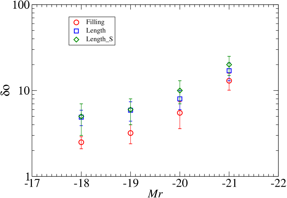
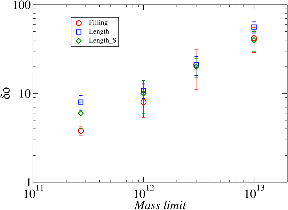
Figure 10: Particle density limit parameter $\delta_{0}$ for SDSS luminosity limited samples is in left panel, and for halo mass limited HR4 model samples in right panel. Absolute magnitude and halo mass limits are used as arguments. Red circles are based on filling factor test for clusters and voids, blue boxes from length functions test, and green diamonds from length function shape estimates, as given in Table 4.

At high luminosities (halo masses) the largest clusters at small smoothing lengths are shorter than the total length of the sample, as seen in plots of density fields of samples L512.5 and SDSS.19 in Fig. 14. For SDSS and HR4 samples with no percolation we applied cluster lengths at threshold density $D_{t}=0.1$, using interpolation schemes similar to interpolation of filling factor functions. This procedure was applied for high luminosity samples SDSS.20 and SDSS.21, and for high-mass samples HR4.12, HR4.123, and HR4.13. Results of this interpolation are shown in right panels of Fig. 9. We used locations of length functions for smoothing kernels $R_{B}=1$ and $R_{B}=2$ $h^{-1}$ Mpc. Errors were calculated from the scatter of individual values for different smoothing kernels. Results for particle density limits are given in column (3) $(\delta_{0})_{L}$ of Table 4 for SDSS and HR4 samples.

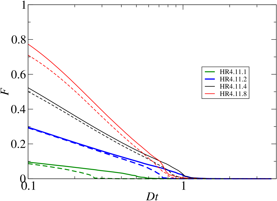
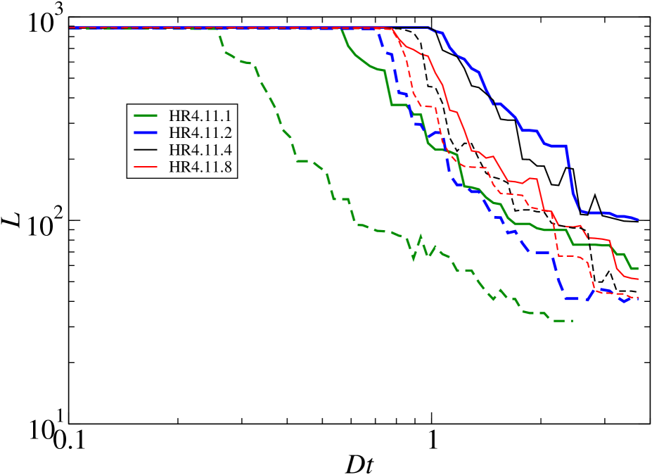
Figure 11: Percolation function tests to check the influence of redshift space distortions. Left panel shows filling factor functions and right panel length functions of HR4.11 models. Solid lines are calculated for real space, dashed lines for redshift space.

One possibility to get simple estimates of positions of SDSS (and HR4) samples relative to L512 samples is to use the general shape of cluster length functions. Here we compare the shape and location of length functions for smoothing kernels $R_{B}=1,\leavevmode\nobreak\ 2$ $h^{-1}$ Mpc with the shape and location of length functions for larger smoothing kernels. For instance, let us compare the length function of the SDSS.18.1 (here the second index 1 shows the smoothing scale, $R_{B}=1$ $h^{-1}$ Mpc) sample relative to SDSS.18 samples for larger smoothing kernels, SDSS.18.2, SDSS.18.4, and SDSS.18.8. Fig. 6 shows that the length function of the sample SDSS.18.1 is located between length functions of samples SDSS.18.4 and SDSS.18.8. Near the percolation level the length function of the model sample L512.2.1 lies to the right of length functions of samples L512.2.2, L512.2.4 and L512.2.8. But in the model sample with higher particle density limit L512.5.1 the length function is located approximately identical to the location of the length function of the L512.5.2 sample.

Comparing locations of SDSS sample length functions at smoothing kernels $R_{B}=1$ $h^{-1}$ Mpc and $R_{B}=2$ $h^{-1}$ Mpc with locations of respective L512 samples we find that the shape of the length function of the SDSS.18 sample corresponds best with the model sample of particle density limit $\delta_{0}=5$. Definitely length functions of the SDSS.18 samples correspond to model samples L512 within particle density limits $3<\delta_{0}<7$. Thus our estimated corresponding model of the L512 series for the SDSS.18 sample is the model with $\delta_{0}=5\pm 2$. This simple length function shape comparison test uses the information for the whole length function, not only at percolation or $D_{t}=0.1$ level. It was made for all SDSS and HR4 samples, results are given in column (4) $(\delta_{0})_{Ls}$ of Table 4.

Length function tests confirm results obtained with the filling factor test. As we see from Table 4, cluster length tests yield a bit higher particle density limits $\delta_{0}$ for SDSS samples than the filling factor test. Fig. 10 shows particle density limit parameter $\delta_{0}$ and its error for all luminosity limited SDSS samples, and for halo mass limited HR4 samples, applying filling function and length function tests. All tests show that the particle density limit of biased model samples increases with the increase of the luminosity (halo mass) of the sample; the increase is regular and has a small scatter. Graphs for SDSS and HR4 samples can be brought to a single diagram if a mass-to-luminosity ratio of SDSS samples, $M/L_{r}=103\pm 10$, is applied.

5.4 Redshift space distortions

Model samples yield true spatial coordinates, observational SDSS samples are based on angular positions and redshifts. In using redshifts to calculate spatial coordinates one must take into account two types of redshift space distortions: the fingers of God effect, caused by random motion of galaxies in clusters, and redshift space distortions (RSD) or the Kaiser (1987) effect, caused by coherent motions of galaxies towards clusters and superclusters.

The finger of God effect is taken into account in catalogues of groups and clusters, used in calculations of the SDSS density field (Tempel et al., 2014). The Kaiser effect leads to an apparent flattening of the structure — pancakes of God. For this reason the SDSS density field is distorted. Filamentary connections between over-density regions are disturbed by the Kaiser effect. Filling factor test functions are shown in Fig. 8, cluster length test functions in Fig.  9. In these Figures filling factors and lengths of L512 model samples represent true model filling factors and lengths. To correct for this effect points corresponding to SDSS samples must be shifted, which leads to changes of particle density limits $\delta_{0}$. The problem is, How much?

In answering this question the comparison of filling factor and length tests of HR4 model samples is of help. The analysis described above was based on true positions of halos in real space. We made a new analysis, using positions and velocities of halos of the HR4.11 sample to a calculate a version of the sample in redshift space. Positions of all halos were shifted from real to redshift space for an observer, located outside of the box by 100 $h^{-1}$ Mpc, at the centre below the $x=y=0$ plane. We calculated percolation functions for both versions of the HR4.11 sample. Results are shown in top panels of Fig. 11, the left panel is for filling factor functions, and the right panel for length functions.

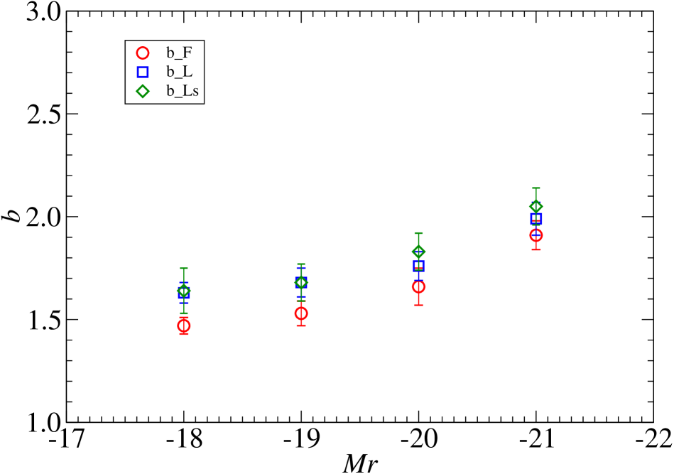
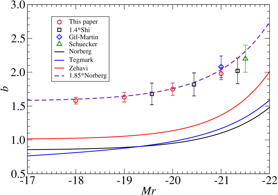
Figure 12: Left panel: bias parameter $b$ values as function of the absolute magnitude limit $M_{r}-5\log h$ of the sample. Red circles show bias parameter values as found from biased L512 spectra using the filling factor test, $b_{F}$, blue boxes indicate bias parameters as found from spectra using the length function test, $b_{L}$, and green diamonds show bias parameters using the length function general shape test $b_{Ls}$. Right panel: Bias function found in this paper compared with bias functions found in other studies. Bias parameter values for SDSS galaxies of various absolute magnitude limits found in this paper are marked by red circles with error bars. Bias parameter values of SDSS galaxies found by Shi et al. (2018) and applying normalising factor $b_{\circ}=1.4$ are marked by black squares with error bars; bias parameter for BOSS galaxies according to Gil-Marín et al. (2017) by blue diamond, and for X-ray clusters of galaxies by Schuecker et al. (2001) by green triangle. Dashed line shows the fit by Norberg et al. (2001), applying bias normalising factor $b_{\circ}=\leavevmode\nobreak\ 1.85$. Black, blue and red lines show fits by Norberg et al. (2001), Tegmark et al. (2004a) and Zehavi et al. (2011).

We used filling factors at threshold density level $D_{t}=0.1$ to find particle density limits of L512 samples, corresponding to HR4 models. This test shows, that for smoothing lengths 1 and 2 $h^{-1}$ Mpc, HR4.11 models in real and redshift space yield practically identical $\delta_{0}$ limits. In the cluster percolation threshold (length) test HR4.11 samples in redshift space yield a mean value $\delta_{0}=9.6\pm 1.9$, which is a bit larger than for real space, $\delta_{0}=8.0\pm 1.5$, see Table 4. If such relative corrections are applied to observed samples, then particle density limits $(\delta_{0})_{L}$ in real space would be $4.1,\leavevmode\nobreak\ 4.9,\leavevmode\nobreak\ 6.7,\leavevmode\nobreak\ 14.1$ for samples SDSS.18, SDSS.19, SDSS.20 and SDSS.21, respectively. Such corrections bring particle density limits $(\delta_{0})_{L}$ closer to limits, found from the filling factor test, $(\delta_{0})_{F}$.

The length function test compares essentially percolation length of samples, the filling factor test the volumes of clusters and voids at very low threshold density $D_{t}=0.1$. Our check using HR4 samples shows that differences found from the comparison of results for real and redshift space are small. Filling factor and length tests represent very different properties of the cosmic web; it is surprising that both tests yield so close results. We can make a tentative conclusion that redshift space distortion effect is small, and that differences of filling factor and length tests of SDSS samples are mainly due to random factors.

5.5 Luminosity dependence

We applied the function (3) with parameter set for $f=0$ to find bias parameter values of biased L512 models, $b_{F}$, $b_{L}$ and $b_{Ls}$, corresponding to SDSS and HR4 samples. Results are given in Table 4. Bias parameter values of SDSS samples are shown in left panel of Fig. 12 as function of the absolute magnitude limit $M_{r}$ of samples. Red circles show $b_{F}$, calculated from L512 spectra for biased models using filling factor test; blue and green symbols show $b_{L}$and $b_{Ls}$, found from spectra of biased L512 models using two length function tests. Errors were found from the mean scatter of $b_{F}$, $b_{L}$ and $b_{Ls}$ values for luminosity limited SDSS samples, as shown in Table 4. We accept an arithmetic mean of our three tests, $b_{F}$, $b_{L}$, $B_{Ls}$, shown by red circles in the right panel of Fig.  12. The accepted error corresponds to a characteristic error from one measurement. It is internal error — possible systematic errors due to the method must be discussed separately.

Available data indicate that the relative bias function $f(L)=b(L)/b_{\circ}$ is approximately constant at low luminosities $L<L_{\ast}$ at level $f(L<L_{\ast}))\approx 0.9$, which leads to $b(L<L_{\ast})\approx 0.9\times b_{\circ}$. The flattening of the $b(L)$ relation at low luminosities $L$ is probably due to the nature of the distribution of faint galaxies. As shown by Tempel et al. (2009), first ranked galaxies have a tendency of cutoff at magnitudes $M-5\log_{10}h\approx-17$ in photometric system of the 2dF survey $b_{J}$. Satellite galaxies can have fainter luminosities, but satellites are located only around main galaxies (Einasto et al., 1974b). Thus power spectra and percolation properties of very faint galaxies cannot be very different from properties of galaxies corresponding to the faint end of the luminosity function of ventral galaxies.

The luminosity dependence of our data are very well fit by Norberg et al. (2001) bias function

$$f(>L)=b(>L)/b_{\circ}=0.85+0.15(L/L_{\ast}),$$ (5)

where $L$ is the luminosity limit of galaxies of the sample, $L_{\ast}$ is the characteristic luminosity of the sample (Schechter, 1976), and $b_{\circ}$ is the bias normalising factor. Fitting our bias parameters for SDSS samples to the Norberg et al. (2001) bias function yields a normalising factor $b_{\circ}=1.85\pm 0.15$, and we get for the luminosity dependence of SDSS galaxies:

$$b(>L)=1.85\times(0.85+0.15(L/L_{\ast})).$$ (6)

The error was found from the scatter of tests for $b_{F}$, $b_{L}$, $B_{Ls}$. Norberg et al. (2001) defined the relative bias function so that $f(L_{\ast})=1$. Thus our analysis suggests for the bias parameter of $L_{\ast}$ galaxies is $b_{\ast}=1.85\pm 0.15$.

Our bias function is based on the comparison of power spectra of biased model samples L512.i and full model sample L512.00. Since the comparison is differential, possible errors in cosmological parameters of the model are minimal. The critical element of the method is the sharp density limit $\delta_{0}$ used to select particles for biased samples. We checked the influence of sharpness of the density limit using fuzzy limits. However, there remains the question: How well such biased model samples represent luminosity limited SDSS galaxy samples? It is possible that sharp particle density limit and sharp SDSS galaxy luminosity limit yield slightly different samples near lower borders of limits.

We can check possible differences using number functions. Fig. 7 shows that at low and medium threshold densities $0.1\leq D_{t}\leq 1$ and small smoothing lengths number functions of all biased model samples and luminosity limited SDSS samples are almost flat. In this threshold density interval samples are dominated by small isolated clusters, practically identical for the same sample at various threshold density levels, thus the number of clusters remains the same. In samples with larger smoothing length the number of clusters at low $D_{t}$ is smaller, because smoothing joins these isolated clusters at low threshold limit to filaments, and isolated clusters almost disappear. At threshold density $D_{t}=0.1$ and smoothing length $R_{B}=8$ $h^{-1}$ Mpc samples SDSS.18 and L512.2 contain only a few isolated clusters due to faint galaxy filaments connecting knots to single objects. In samples of higher limiting luminosity or particle density limit the number of clusters at $D_{t}=0.1$ gets larger, since filaments connecting knots became invisible, see Fig. 7. In this respect simulated and real galaxy samples yield qualitatively very similar results. We may conclude that our method to find biased model samples using sharp particle density limits is a fair representative to SDSS luminosity limited samples.

As discussed above, redshift space distortions can increase length function test parameters $(\delta_{0})_{L}$ and corresponding bias parameters $b_{L}$. Thus, if one prefers the filling factor test, one can use for the bias parameter of $L_{\ast}$ galaxies a value, $b_{\ast}=1.70\pm 0.15$. This does not influence our main conclusion that the bias parameter of $L_{\ast}$ galaxies is $b_{\ast}\gg 1.0$.

5.6 Comparison with other data

In the right panel of Fig. 12 we compare our results for the bias function $b(L)$ with results by other authors. Dashed line shows our bias function (6). Black, blue and red lines show fits by Norberg et al. (2001), Tegmark et al. (2004a) and Zehavi et al. (2011).

Tegmark et al. (2004a) calculated power spectra in six bins of absolute magnitude, and found that the relative bias function is better given by the expression: $f(L)=b(L)/b_{\circ}=0.895+0.150(L/L_{\ast})-0.040(M-M_{\ast})$, see their Figs. 28 and 29. Here $M_{r}=M_{\ast}-2.5\times\log_{10}(L/L_{\ast})$ and $M_{\ast}$ are $r-$magnitudes of SDSS galaxies and respective Schechter magnitudes.

Zehavi et al. (2011) investigated the galaxy clustering of the completed SDSS survey, and found for the bias function the form $b_{g}(>L)\times(\sigma_{8}/0.8)=1.06+0.21(L/L_{\ast})^{1.12}$, where $L$ is the $r-$band luminosity corrected to $z=0.1$, and $L_{\ast}$ corresponds to $M_{\ast}=-20.44\pm 0.01$ (Blanton et al., 2003). Pollina et al. (2018) found relative linear bias factors between clusters and galaxies using first years of observations of the Dark Energy Survey, $b_{\mathrm{cl}}/b_{\mathrm{gal}}=1.6$ for $L>0.5L_{\ast}$ galaxies.

Shi et al. (2016, 2018) developed a method to map real space distribution of galaxies. The method was applied to measure clustering amplitude of matter and bias parameters of flux-limited sample of galaxies in SDSS DR7 in redshift range $0.01\leq z\leq 0.2$. We show in Fig. 12 the bias parameter values, found by Shi et al. (2018) and applying normalising factor $b_{\circ}=1.4$.

Gil-Marín et al. (2015, 2017) investigated the clustering of galaxies in the SDSS-III Baryon Oscillation Spectroscopic (BOSS) Survey. The BOSS survey selects LRG galaxies and consists of near and distant samples, the LOWZ sample of effective redshifts $z_{LOWZ}=0.32$, and the distant sample CMASS with $z_{CMASS}=0.57$. Gil-Marín et al. (2017) found the linear biasing parameter $b_{1}=2.08$ for LOWZ survey, and $b_{1}=2.01$ for CMASS survey. Gil-Marín et al. (2017) compared observed bias parameters with bias parameters for $N$-body halos of mock samples: low-bias model with halo mass limit $M_{min}=3.80\times 10^{12}\leavevmode\nobreak\ M_{\odot}h^{-1}$ has $b_{1}=1.75$, and high-bias model with $M_{min}=8.36\times 10^{12}\leavevmode\nobreak\ M_{\odot}h^{-1}$ has $b_{1}=2.07$; see Table 1 by Gil-Marín et al. (2017). These values are close to bias parameter values found for our HR4.123 and HR4.13 samples, see Table 4 and Fig. 3. We show in Fig. 12 the bias parameter for BOSS LOWZ galaxies according to Gil-Marín et al. (2017). BOSS galaxies were selected using LRG galaxies. We found for these galaxies the mean red magnitude $M_{r}-5\log h=-21.0$, with a spread about one magnitude. Our SDSS galaxy samples contain galaxies with luminosities greater or equal to absolute magnitude limits. Thus we can accept for LRG galaxies the magnitude limit $M_{r}-5\log h=-20.5$, almost equal to the magnitude of $L_{\ast}$ galaxies.

Power spectra of X-ray detected clusters of galaxies were derived in the framework of REFLEX survey by Schuecker et al. (2001). Power spectra have a maximum around $k=0.05\leavevmode\nobreak\ h$ Mpc^-1, shown in Fig. 2 for two flux-limited cluster samples, L050 with X-ray luminosity limit, $L_{X}\geq 0.5\times 10^{44}$ erg s^-1, and L120 with limit $L_{X}\geq 1.2\times 10^{44}$ erg s^-1. The amplitude of the spectrum is higher for higher X-ray limit clusters. Both spectra correspond to our model samples with very high particle density limit $\delta_{0}\approx 50$; see Fig. 2. For X-ray clusters we estimated the mean magnitude $M_{r}-5\log h=-21.5$.

6 Discussion

We show in Fig. 13 power spectra of L512 models again; the spectrum for biased model L512.10 is highlighted by red colour. This biased model corresponds approximately to $L_{\ast}$ luminosity limited galaxy samples. We show in Fig. 13 also the power spectrum obtained by Tegmark et al. (2004a) according to their Table 3, which corresponds to $L_{\ast}$ SDSS galaxies.

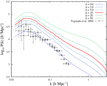
Figure 13: Power spectra of particle density limited L512 model spectra. The power spectrum of the sample L512.10 is shown by bold red line. With filled symbols we show the power spectrum of SDSS galaxies by Tegmark et al. (2004a).

When the presence of the cosmic web was first discussed in the IAU Tallinn Symposium, Zeldovich in his talk emphasised the importance to develop statistical tools to measure quantitatively the new phenomena: the filamentary character of the galaxy distribution and the presence of voids. So far the basic quantitative descriptor of the distribution of galaxies was the two-point projected correlation function $w_{p}(r_{p})$. This function was adequate to describe two-dimensional data, as presented by Seldner et al. (1977) and analysed by Soneira & Peebles (1978). Following this initiative Zeldovich et al. (1982) applied the percolation analysis to test the filamentarity of the web, and the multiplicity analysis to test the clustering properties. The Soneira & Peebles (1978) model failed in both tests. The Zeldovich own model, based on a HDM simulation by Doroshkevich et al. (1982)), failed in multiplicity test. Both tests showed the agreement of model with observations only when a CDM model was used (Melott et al., 1983).

The cosmic web is very rich in details and has complex properties. For this reason there exists no statistical tools which can describe all properties of the web. Each statistical tool is an instruments to test certain well fixed properties of the web. To evaluate possible strengths and limits of power spectrum determinations by various authors we have to understand what features of the web can be tested by particular tools. General properties of the cosmic web as delineated by galaxies and DM are known long ago. As discussed above, the main difference between distributions of matter and galaxies is the presence of DM in low-density regions, with no corresponding population of galaxies.

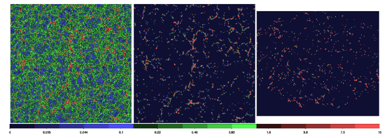
Figure 14: Left and central panels show high-resolution non-smoothed density fields of identical $512\times 512\times 1$ $h^{-1}$ Mpc slices of dark matter models L512.00, L512.10, found for particle density limits $\delta_{0}=0,\leavevmode\nobreak\ 10$. Right panel shows central section of the non-smoothed density field of the SDSS.21 galaxy sample. This Figure illustrates the effect of zero density regions in simulated and real density fields of galaxies. Densities are expressed in logarithmic scale in interval 0.005 to 15 in mean density units. The colour code is identical in all panels.

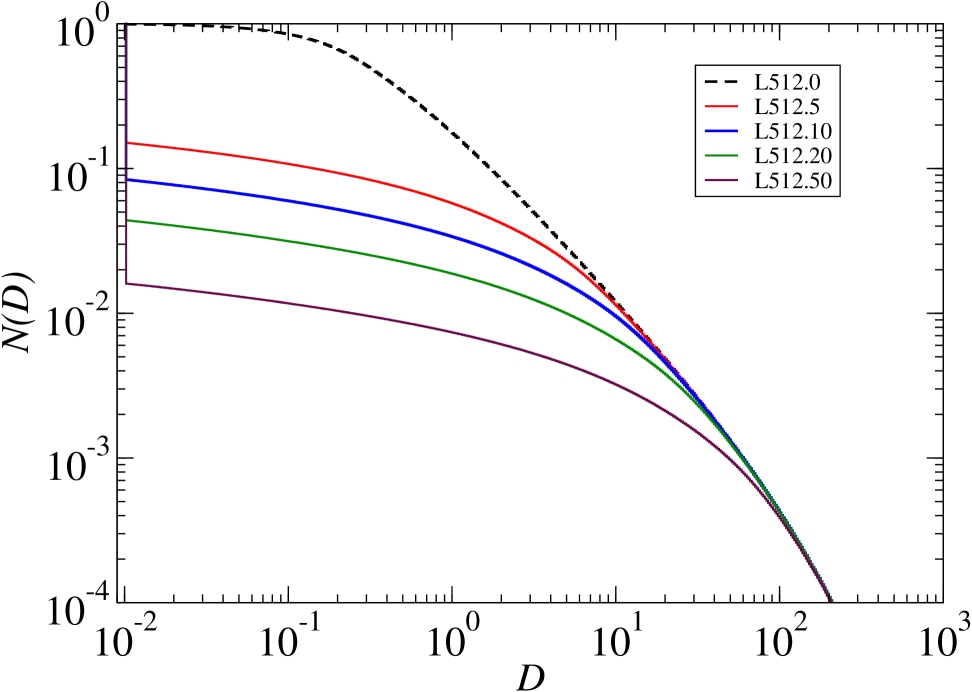
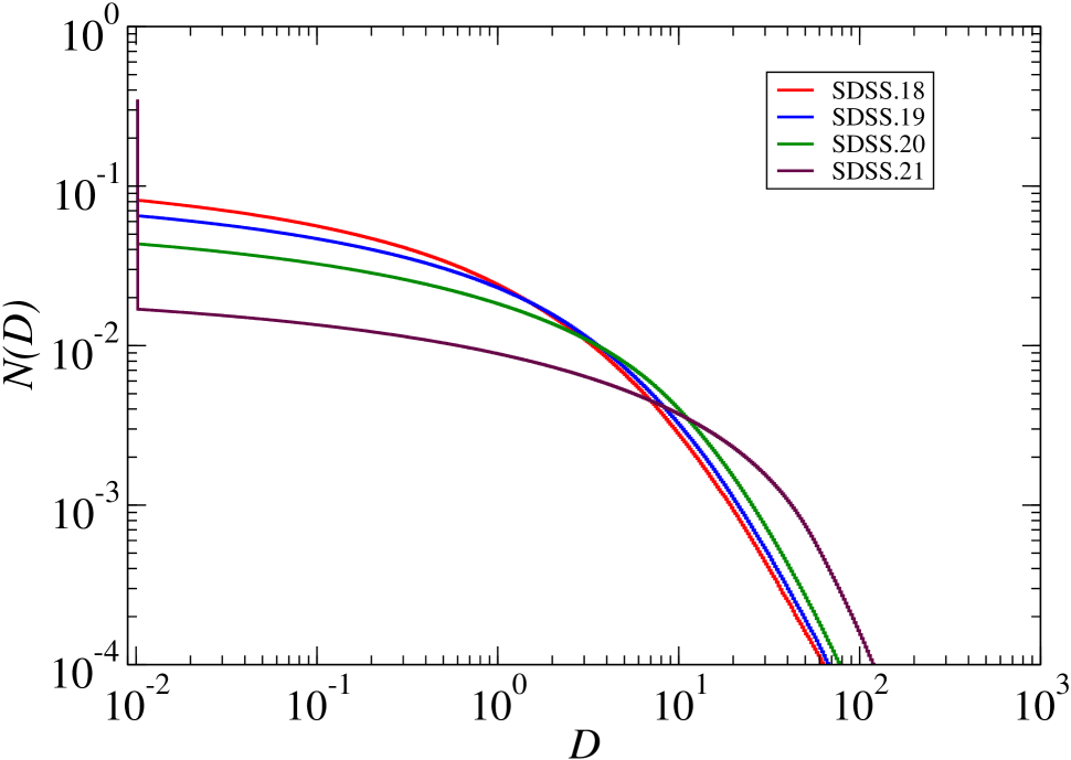
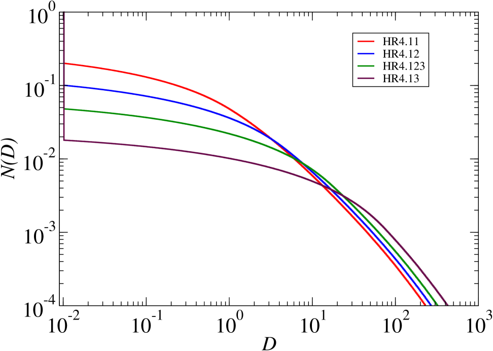
Figure 15: Cumulative distributions of densities in L512, SDSS and HR4 samples, left, middle and right panel respectively.

Geometrical properties of density fields of matter, model galaxies, and SDSS galaxies were discussed in previous Sections. Here we discuss some aspects of the distribution, critical to power spectrum analysis. In Fig. 14 we compare high-resolution density fields of these samples, represented by the full model sample L512.00, the biased model sample L512.10, and the SDSS.21 sample. $L_{\star}$ galaxies have approximately the magnitude $M_{r}-5\log h=-20.5$, thus the luminosity density field of SDSS.21 contains a bit higher luminosity galaxies than the L512.10 field. The Figure shows that qualitatively the pattern of the distribution of simulated and real clusters is similar. The presence of large regions with zero spatial density is well seen in simulated and real galaxy density fields.

In Fig. 15 we compare cumulative distributions of densities in density fields of model samples L512 with respective distributions for observed SDSS samples and comparison HR4 samples. For the L512 model distributions are shown for the full sample with all particles, L512.00, and for biased model samples L512.5, L512.10, L512.20 and L512.50. In the full sample there are particles with all density labels, thus the cumulative distribution approaches unity with decreasing particle density smoothly. In all biased samples low-density particles are absent, thus a large fraction of cells of the density field have zero density. The cumulative distribution has a peak at lowest density value, corresponding to pixels with zero density, and continues at lower level. Density distributions of SDSS and HR4 samples are qualitatively similar to distributions of biased L512 samples.

Figure 16 shows a cross sections of the density field at spatial $y,z$-coordinates through the center of the field, presented in Fig. 14. We plot here the density contrast $\delta(x)=D(x)-1$. Blue line shows the density contrast at the early epoch, corresponding to redshift $z=30$. At this early epoch the amplitude of density fluctuations is small, density fluctuations are approximately equal everywhere. Black line gives the density contrast for the same cross section at the present epoch for the sample with all particles, L512.00, and red line for the biased sample L512.10.

In the sample L512.10 high-density peaks of the density field of biased models are the same as in the full model. Weak DM knots of medium density, seen in the sample L512.00, are gone. In low density regions with $\delta<6$ the density contrast of the L512.00 sample fluctuates between values $0<\delta<6$ with a mean around $\delta=-0.5$. Over most of the density field the density of the sample L512.10 has zero density and density contrast $\delta=-1$.

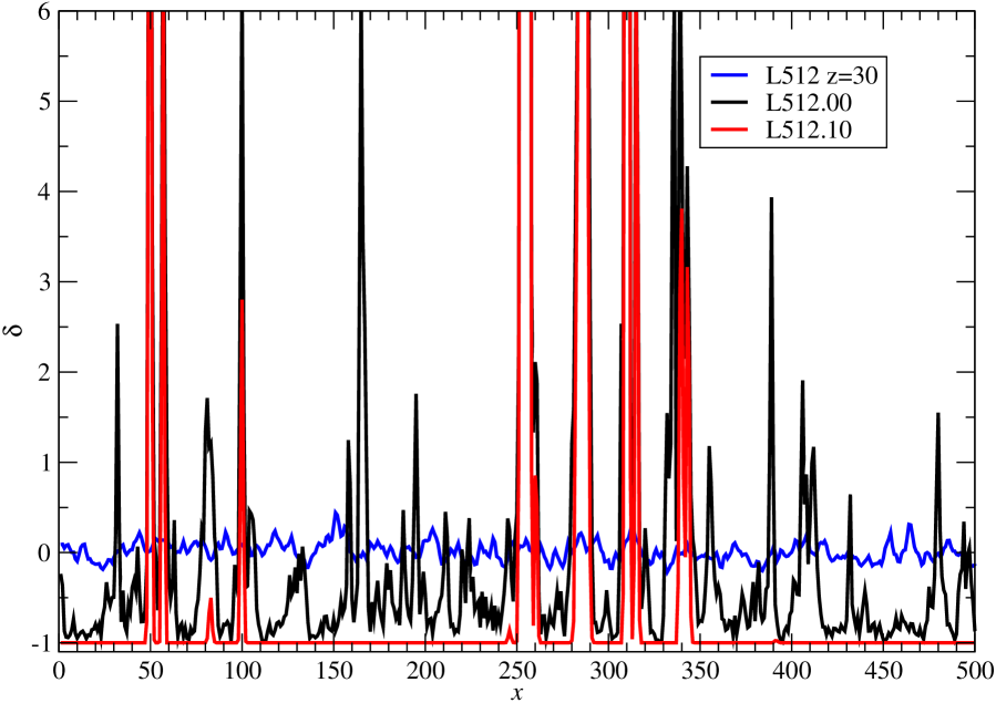
Figure 16: Cross sections of the density contrast $\delta(x)=D(x)-1$ of the model L512 along the $x$-spatial coordinate at the same $z$-coordinate as shown in Fig. 14. Blue line shows the density field of the model L512.00 at redshifts $z=30$. Black line shows the density field of the full model L512.00 at the present epoch, and red line for the biased model L512.10.

We give in Table 1 the fraction of particles in biased samples, $F_{C}$, and filling factor $FF_{C}$ of all clusters (non-zero density cells) of the density field at threshold density $D_{t}=0.1$. Both quantities are given as functions of the particle density limit $\delta_{0}$ of biased model samples. The Table shows that the filling factor of clusters decreases with increasing $\delta_{0}$ much faster than the fraction of particles. This is a well-known effect: the density of clusters increases towards their centres and the volume decreases more rapidly than the number of particles. For comparison we note that filling factors of all clusters at the threshold density level $D_{t}=0.1$ of samples SDSS.18, SDSS.19, SDSS.20 and SDSS.21 are 0.1795, 0.1449, 0.0976 and 0.0399, respectively. The fraction of zero density cells is respectively increasingly closer to unity when we increase the sample particle density limit $\delta_{0}$ or the luminosity limit $L$. In the sample L512.10 95% of all cells of the density field have zero density, in the SDSS.21 field even 96% of cells.

In our method power spectra are calculated using $\Lambda$CDM models. Power spectrum is a sum over all density contrasts. The sum is the larger the greater is the fraction of cells with zero density and density contrast $\delta=-1$. For this reason the power spectrum of all biased model samples has a higher amplitude than the full DM model; the amplitude is the higher the larger the fraction of zero density regions. Thus the power spectrum is a measure of the fraction of zero-density cells in the sample. It is interesting to note that Einasto et al. (1986) received the same conclusion from the analysis of the three-dimensional correlation function.

A summary of measurements of power spectra is presented in Figs. 12 and 13. The power spectrum for our full DM model L512.00 is in very good agreement with the updated matter power spectrum at $z=0$, as compiled by Chabanier et al. (2019). The comparison of various determinations shows that all methods permitted to determine very accurately the luminosity dependence of galaxy power spectra, when appropriate bias normalising factors $b_{\circ}$ are applied. The amplitude of the spectrum can be characterised by the bias normalising factor. Figures show that normalising factors can be divided into two groups: around $b_{\circ}\approx 1$ — Norberg et al. (2001), Tegmark et al. (2004a) and Zehavi et al. (2011); and around $b_{\circ}\approx 2$ — Schuecker et al. (2001), Gil-Marín et al. (2015, 2017) and our work. This variety of bias normalising factors suggests that authors used different tools to handle zero density regions of the luminosity density field of galaxies.

Devil is in detail. Methods to estimate power spectra of galaxies contain numerous technical details and assumptions. Each method yields results what the method permits. In this respect a combined method using different properties of the cosmic web has an advantage to see the bias phenomenon in a broader context. It is clear that future development adds new details to the picture we have today.

7 Concluding remarks

The present study shows that the absence of galaxy formation in low-density regions of the cosmic web is an essential property of the $\Lambda$CDM universe. It follows from the combined action of several physical processes: (i) the smoothness of the flow of particles until the intersection of particle trajectories; (ii) the formation of halos along caustics of particle trajectories; (iii) the phase synchronisation of density perturbations of various scales; and (iv) the two-step nature of galaxy formation by condensation of baryonic matter within DM halos.

We studied the distribution of galaxies and matter using respective density fields and applying percolation and power spectrum analyses. To calculate the density fields of simulated galaxies we used the particle local density $\delta$ as a dimensionless characteristic of particles of numerical simulations of the cosmic web. We applied sharp particle density limit, $\delta\geq\delta_{0}$, to select particles, which form biased model samples. We tested this selection algorithm using fuzzy particle density limits and analysing number functions of simulated and real galaxies. Our analysis shows that this sample selection method yields biased model samples in a wide range of particle density limits, and allows to calculate bias function of biased model samples as functions of the particle density limit, $b(>\delta_{0})$. The bias function depends on cosmological parameters of the model only weakly, since we use ratios of power spectra of the same model.

We compared biased model samples with luminosity selected SDSS galaxy samples using the extended percolation analysis. Our analysis shows that the extended percolation method allows to compare observational and model samples having very different sample sizes and configurations. The method is almost not influenced by redshift space distortions, present in observational samples. The percolation method is very sensitive to geometrical properties of clusters and voids of observed and model samples, and allows to find density limits $\delta_{0}$ of biased models, which correspond to luminosity limited SDSS samples..

As a result of physical processes described above there exists at all cosmological epochs a low-density population, consisting of a mixture of dark and baryonic matter. A crucial role in the evolution of the universe plays the phase synchronisation which leads to the formation of small filamentary high-density regions and large contiguous regions with very low spatial densities. Galaxy formation is possible only in the high-density medium. This is the main factor in the biasing phenomenon, leading to increase of zero density cells in density field of simulated and real galaxies, and an increase of the amplitude of the power spectrum of galaxies in respect to the power spectrum of matter. The second largest effect is the dependence of the bias function on the luminosity of galaxies. Variations in gravitational and physical processes during the formation and evolution of galaxies, represented in our biasing model by the fuzziness of the biasing threshold, have the smallest influence.

The combined geometrical and power spectrum analysis demonstrates well the presence of large differences between distributions of matter and galaxies, expressed quantitatively by percolation functions and power spectra. Power spectra of biased models representing SDSS samples of various luminosity limits allowed to calculate the expected bias function, $b(>L)$. The bias function is in very good agreement with earlier studies when appropriate bias normalising factors are applied.

Our main conclusions are.

1. Non-clustered matter in low-density regions is smoothly distributed, which rises the amplitude of power spectra of the clustered matter in galaxies in respect to the amplitude of power spectra of all matter. This is the dominant factor to influence the biasing phenomenon, and can be used as a cosmological constraint.

2. The dependence of the bias parameter on the luminosity of galaxies is the second largest effect affecting the bias parameter. Variations in gravitational and physical processes during the formation and evolution of galaxies have the smallest influence to the bias parameter.

3. Combined analysis of geometrical properties of the cosmic web and power spectra of biased model samples and SDSS samples of galaxies allow to estimate the bias parameter of $L_{\ast}$ galaxies, $b_{\ast}=1.85\pm 0.15$.