Elliptic flow of identified particles in Pb-Pb collisions at $\sqrt{s_{NN}}=5.02$ TeV

Abstract

In this paper, by using a Tsallis-Pareto-type function and the multisource thermal model, the elliptic flow coefficients of particles $\pi^{\pm}$, $K^{\pm}$, $p+\overline{p}$, $\Lambda+\overline{\Lambda}$, and $K_{S}^{0}$ produced in Pb-Pb collisions at the center-of-mass energy of $\sqrt{s_{NN}}=5.02$ TeV are investigated. In the process of collisional evolution, because of geometric structure, pressure gradient, and thermal diffusion effects, deformation and translation occurred in the isotropic emission source, leading to anisotropy in the azimuth distribution of the final-state particles. Based on these dynamic factors, the dependence of elliptic flow on transverse momentum is described as well.

PACS: 14.65.Bt, 13.85.Hd, 24.10.Pa

I Introduction

As collision energy has gradually increased in recent years, high-energy physics has developed rapidly. On the one hand, the energy range of nucleus-nucleus collisions has been broadened 1 ; 2 ; 3 ; 4 . On the other hand, the kinds of final-state particles measured by detectors have become more explicit 5 ; 6 ; 7 . This creates better conditions for obtaining a deep understanding of the collision mechanism. The distribution of high-energy final-state particles is important to understand the evolutionary mechanism of fluid dynamics, where as the flow effect of final-state particles is meaningful for the new material form, quark-gluon plasma (QGP) 8 ; 9 ; 10 . The formation of QGP requires an extremely high-temperature, high-density environment. It is a state of released quarks and gluons that is similar to an ideal fluid. From an anisotropic azimuth analysis of final-state particles measured at the Relativistic Heavy Ion Collider (RHIC) 11 and the Large Hadron Collider (LHC) 12 , it can be seen that the generated material unaffected by gravity is QGP under the condition of strong coupling. The quarks and gluons in the high-temperature, high-density state are affected by multiple factors. By means of the pressure gradient, the heterogeneity of energy density and the asymmetry of the geometric structure at the early stage of collisions are converted to the anisotropy of final-state particle momentum and finally manifest as the flow effect 121 ; 122 .

In the evolutionary process of high-energy collisions, there are two main stages, chemical freeze-out and dynamic freeze-out. The former occurs in the formation stage of different kinds of particles, and the decay and generation of particles remain in dynamic balance. This is an inelastic collision process. The second process occurs later, in the diffusion stage. Momentum and energy are maintained in a thermal equilibrium state in an elastic collision process. After the two stages, as the temperature drops, the final-state particles are ejected from the action system. Various physical properties of the final-state particles are then measured by detectors, such as the longitudinal momentum spectrum 13 ; 14 , the rapidity (pseudorapidity) distribution 15 ; 16 , the multiplicity distribution 17 ; 18 , and the flow effect 19 ; 20 ; 101 ; 102 ; 103 ; 104 ; 105 ; 106 ; 107 ; 108 . By analysis of the final-state distribution using various theoretical models, the dynamic evolutionary mechanism, phase graph information, and particle attribution of quantum chromodynamics were deduced.

In non-central nucleus-nucleus collisions, the main coefficient of the flow effect is the second-order harmonic, which is called elliptic flow ($v_{2}$). The value is used to represent collective motion in the system. Collective motion is one of the characteristics formed in collisions of QGP. The flow effect that is caused by the asymmetry of the initial geometric structure and the heterogeneous energy of the action system includes direct flow, elliptic flow, and triangular flow. All the harmonics are quantified by the coefficient ($v_{n}$) of Fourier decomposition 21 ; 22 :

$$\frac{dN}{d\varphi}\varpropto 1+2\sum v_{n}\cos\left[n(\varphi-\Psi_{n})\right],$$ (1)

Similar long-range ridge structures and positive coefficients $v_{2}$ have been observed in experiments 19 . In theory, it is assumed that these are based on the collective effect caused by hydrodynamic evolution of colliding particles.

Previous studies 231 ; 232 ; 233 have presented a description of elliptic flow over a smaller range. Moreover, the isotropic hypothesis on the transverse plane and the translation and expansion effects of the emission source are used. In this paper, based on the multisource thermal model, using the distribution of the Tsallis-Pareto-type function, and at the center-of-mass energy of $\sqrt{s_{NN}}=$5.02 TeV, the dependence of the elliptic flow of the identified particles ($\pi^{\pm}$, $K^{\pm}$, $p+\overline{p}$, $\Lambda+\overline{\Lambda}$, and $K_{S}^{0}$) in different centrality intervals in Pb-Pb collisions on transverse momentum is described 24 . The multisource thermal model is a statistical model that is based on the one-dimensional string model 301 and the fireball model 302 and was developed from the thermalized cylinder model 303 ; 304 . According to the multisource thermal model, many local emission sources are formed along the incident direction in high-energy collisions, and the final-state particles and jets are generated by these emission sources. In the rest frame of an emission source, the source is isotropic, that is, the final particles produced by the emission source are assumed to emit isotropically. Due to differences in impact parameters, centralities, position in space, or energy density, the emission source’s temperature, excitation degree, and particle yield ratio may vary. In comparison with previous work 231 ; 232 ; 233 by the multisource thermal model, not only is the range of transverse momentum larger, but also the identification of the final-state particles is more accurate.

II Model and formulation

In this paper, using the multisource thermal model 25 ; 26 ; 27 ; 28 ; 29 and a Tsallis-Pareto-type function 30 ; 31 ; 32 ; 33 , the elliptic flow of identified particles in Pb-Pb collisions is analyzed. For each source in the multisource model, the Tsallis-Pareto-type function shows excellent reproducibility of the spectral measurement of many particles; the form is:

$$\frac{d^{2}N}{dydp_{T}}=\frac{dN}{dy}Kp_{T}\left[1+\frac{m_{T}-m_{0}}{nC}\right]^{-n},$$ (2)

where

$$K = \frac{(n-1)(n-2)}{nC\left[nC+(n-2)m_{0}\right]},$$ (3)

$$m_{T} = \sqrt{m_{0}^{2}+p_{T}^{2}},$$ (4)

where $m_{0}$ is the rest mass, $y$ is the rapidity, and $N$ is the number of particles. According to some non-extensive thermodynamic particle models, the free parameter $C$, which is related to the average particle energy, represents the mean effective temperature in the interacting system, $dN/dy$ is the particle output at different rapidity intervals, and $n$ indicate the non-extensivity of the process, which is the departure of the spectra from the Boltzmann distribution. After integrating for rapidity, the distribution density function of the transverse momentum is:

$$f(p_{T})=\frac{dN}{dp_{T}}=N_{0}Kp_{T}\left[1+\frac{m_{T}-m_{0}}{nC}\right]^{-n},$$ (5)

where $N_{0}$ denotes the normalization constant, which depends on the free parameters $n$ and $C$. Hence, it is natural that $\int\nolimits_{0}^{\infty}f(p_{T})dp_{T}=1$.

Related work 34 has shown that the transverse momentum distribution of the final-state particles formed in nucleus-nucleus collisions satisfies the Tsallis-Pareto-type function. In accordance with the Monte Carlo method, by Eq. (5), the transverse momentum $p_{T}$ can be extracted. In this expression, $R_{0}$ represents random numbers uniformly distributed on [0,1], and $p_{T}$ can be given as:

$$\int_{0}^{p_{T}}f(p_{T})dp_{T}<R_{0}<\int_{0}^{p_{T}+dp_{T}}f(p_{T})dp_{T}.$$ (6)

Under the assumption of an isotropic emission source, the azimuth distribution of final-state particles is even, and the distribution function is:

$$f_{\varphi}\left(\varphi\right)=\frac{1}{2\pi}.$$ (7)

By the Monte Carlo method, the random number of the azimuth can be obtained as:

$$\varphi=2\pi R,$$ (8)

where $R$ represents a random number distributed on [0, 1]. Let the beam direction be the $Oz$ axis, and let the reaction plane be the $xOz$ plane. Therefore, the momentum components are

$$p_{x} = p_{T}\cos\varphi,$$ (9)

$$p_{y} = p_{T}\sin\varphi.$$ (10)

Due to the geometric structure of the participant, the pressure gradient, and interaction with the medium, the emission source deforms and translates in its rest frame. Hence, an anisotropic emission source is introduced in the multisource thermal model. To quantify the deformation and translation of the emission source, $a_{x}$ ($a_{y}$) and $b_{x}$ ($b_{y}$) express the deformation and translation of the emission source along the $Ox$ ($Oy$) axis, $a_{x}>1$ ($<1$) represents expansion (compression), and $b_{x}>0$ ($<0$) represents translation along the positive (negative) axis. Generally, for particles with different centrality intervals and transverse momentum, different $a_{x}$ ($a_{y}$) or $b_{x}$ ($b_{y}$) are obtained. As a first approximation, the empirical relationship can be expressed as:

$$a_{x}=1+k_{1}\exp(-\frac{p_{T}}{\lambda_{1}})+k_{2}p_{T},$$ (11)

where $k_{1}$, $\lambda_{1}$, $k_{2\text{ }}$are free parameters. For simplicity, the default is $a_{y}=1$ and $b_{x,y}=0$. Because of deformation, the above $p_{x}$ is revised to become:

$$p_{x}^{\prime}=a_{x}p_{x}+b_{x}.$$ (12)

Then the converted transverse momentum is:

$$p_{T}^{\prime}=\sqrt{p_{x}^{\prime 2}+p_{y}^{2}}.$$ (13)

Finally, the elliptic flow of final-state particles can be represented as:

$$v_{2}=\left\langle\frac{p_{x}^{\prime 2}-p_{y}^{2}}{p_{x}^{\prime 2}+p_{y}^{2}}\right\rangle.$$ (14)

III Comparisons with experimental data

Using the multisource thermal model, the anisotropic spectrum data of various particles generated in Pb-Pb collisions at $\sqrt{s_{NN}}=5.02$ TeV 24  are studied and analyzed. The particles $\pi^{\pm}$, $K^{\pm}$, $p+\overline{p}$, $\Lambda+\overline{\Lambda}$, and $K_{S}^{0}$ are located in different centrality intervals within 0–70% and depend on $v_{2}$ of the transverse momentum $p_{T}$. The rapidity is in the range $\left|y\right|<0.5$. For particles $\pi^{\pm}$, $K^{\pm}$, and $p+\overline{p}$, the measurements in hypercenter collisions (0–1%) are also shown.

Figure 1 shows the elliptic flow $v_{2}(p_{T})$ of meson $\pi^{\pm}$ generated in a Pb-Pb collision at energy $\sqrt{s_{NN}}=5.02$ TeV in different centrality intervals. The data measured by the ALICE Collaboration in different centrality intervals are represented by different solid symbols, and the statistical and systematic errors are both considered in the error bar 24 . The curves are fitted to results generated by the Tsallis-Pareto-type function in the framework of the multisource thermal model. Table 1 shows the fitted free parameters ($C$, $n$, $k_{1}$, $\lambda_{1}$, and $k_{2}$), $\chi^{2}$ and the degrees of freedom (dof). Clearly the model results are consistent with the experimental data. In the calculation, the data fitting indicates that the effective temperature $C$ increases as the centrality percentage decreases, but that the value of $n$ remains unchanged and is assumed to be 9. It is obvious that $v_{2}$ increases with $p_{T}$ in the low $p_{T}$ region, and then decreases slowly in the high $p_{T}$ region. The transverse momentum corresponding to the maximum value increases with increasing particle mass. This trend is reflected in the values of $k_{1}$, $\lambda_{1}$,  and $k_{2}$. Moreover, it is not hard to find that the parameter $k_{1}$ first increases rapidly with the centrality percentage and then slowly decreases. Finally, the values of $\chi^{2}/dof$ are in a reasonable range, which is not only affected by experimental errors, but is also related to the inaccuracy of the theoretical calculation results.

Figure 2 shows that $v_{2}(p_{T})$ of $K^{\pm}$ in the given centrality interval. Similarly to Fig. 1, the solid symbols also represent the experimental data recorded by the ALICE Collaboration, and the error bar includes the statistical and systematic errors. The curves are the results of fitting using the Tsallis-Pareto-type function. The fitting parameters, $\chi^{2}$ and dof are also listed in Table 1. It is apparent that the experimental data are well fitted by the model results. In the calculation, the values of effective temperature $C$ decrease from the central to peripheral collisions and are systematically larger than those for particles $\pi^{\pm}$. As the centrality percentage increases, the values of $k_{1}$ first increase rapidly, then slowly decrease, as shown in Fig. 1.

Figure 3 shows the $v_{2}$ of $p+\overline{p}$, which depends on the transverse momentum. Figures 4 and 5 show the relationship between the elliptic flow and the transverse momentum spectrum of $\Lambda+\overline{\Lambda}$ and $K_{S}^{0}$ respectively. The solid symbols are the data points, and the curves show the model results. The fitted parameter values, dof and $\chi^{2}$, are included in Table 1. It is evident that the fits are in good agreement with the experimental data. However, as shown in Fig. 4, in the given centrality interval of 60–70%, there is a datum point located at $p_{T}=9$ Gev/c that deviates seriously from the fitted value. The physical mechanism underlying this deviation is not yet understood. Similarly, when moving from central to peripheral collisions, $C$ increases, and $k_{1}$ increases rapidly, then decreases slowly. Overall, the model fits the spectrum $v_{2}(p_{T})$ of identified particles measured in different centrality intervals by ALICE in Pb+Pb collisions at approximately $\sqrt{s_{NN}}=5.02$ TeV.

Based on the fitted results shown in Figs. 1–5, Figure 6 shows the dependency relationship between the expansion factor $a_{x}$ and the transverse momentum $p_{T}$ in the given centrality interval for different particles $\pi^{\pm}$, $K^{\pm}$, $p+\overline{p}$, $\Lambda+\overline{\Lambda}$, and $K_{S}^{0}$. For a certain particle, $a_{x}(p_{T})$ are different in different centrality intervals. The curves with maximum and minimum dependency relationship were chosen based on Eq.(11) and are represented by solid and dashed lines respectively. The variation trends are similar, but the ranges are slightly different. Furthermore, as the particle mass increases, the range also increases. Figure 7 shows the fitting parameter $C$, which depends on the variation of centrality. When moving from central to peripheral collisions, the effective temperature $C$ gradually declines.

IV Discussion and conclusions

According to the fitted results from the above comparisons, the fitted free parameter $C$ is actually not the real temperature (the kinetic freeze-out temperature) of the emission source, but the effective temperature. As is well known, the interacting system at kinetic freeze-out (the last stage of collision) is influenced not only by thermal motion, but also by the flow effect. The real temperature of the emission source should reflect the thermal motion of the particles, and therefore the real temperature of the source is the kinetic freeze-out temperature. The effective temperature extracted from the elliptic flow spectrum includes thermal motion and the flow effect of the particles. By dissecting the effective temperature, it is possible to obtain the real temperature of the interacting system. The relationships between effective temperature, real temperature, and flow velocity are not totally clear. Therefore, the value of effective temperature obtained in this work is higher than the kinetic freeze-out temperature.

Table 1 shows that the parameter $k_{1}$ first increases rapidly with centrality percentage and then decreases slowly. It reaches a maximum as the centrality percentage reaches about 30%. In addition, Fig. 6 shows that $a_{x}$ decreases with increasing transverse momentum $p_{T}$. However, Fig. 7 shows that the parameter $C$ declines gradually from central to peripheral collisions. As for the dependency relationship, it can be readily understood.

From the participant-spectator geometric structure, it can be seen that as centrality percentage increases, the extent of the overlapping parts decreases, whereas the asymmetry rises. There is an approximate linear relationship between the elliptic flow and the eccentricity ratio of the participant. Hence, with increasing centrality percentage, the elliptic flow also grows. However, $v_{2}$ of particles in peripheral collisions is slightly smaller than in central collisions. This may be due to shorter system life under peripheral collisions, resulting in small $v_{2}$. Hence, $k_{1}$ first increases rapidly with the centrality percentage and then decreases slowly.

However, as the centrality percentage rises, the effective temperature $C$ declines gradually. In accordance with the geometric structure of collisions, as the centrality percentage decreases, the number of involved nucleons increases, and the overlapping parts also increase, leading to higher energy density and strength of interaction, which manifests as higher temperature. The effective temperature $C$ obtained in this study was higher than the true temperature. The reason for this was that the effective temperature incorporates the true temperature and the flow effect. The value excluding the flow effect should be equal to the true temperature. Fig. 7 shows that for particles with considerable mass, the low variation ranges of effective temperature are similar.

In short, based on the multisource model, by introducing a Tsallis-Pareto-type function, the elliptic flow of identified particles generated in Pb-Pb collisions at $\sqrt{s_{NN}}=5.02$ TeV was correctly analyzed. Therefore, in the collision process, the asymmetry, expansion, and translation effects of geometric structure affect the dynamics of the final-state particles.

Data Availability

The data used to support the findings of this study are included within the article.

Ethical Approval

The authors declare that they are in compliance with ethical standards regarding the content of this paper.

Conflicts of Interest

The authors declare that they have no conflicts of interest regarding the publication of this paper.

Table 1. Values of $C$, $n$, $k_{1}$,$\lambda$₁,$k_{2}$, $\chi^{2}$ number of degrees of freedom (dof) corresponding to the fits in Figs. 1–5.

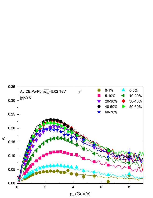
Figure 1: $v_{2}(p_{T})$ of $\pi^{\pm}$ in a given centrality interval arranged into panels of various centrality classes 24 . The data, which were measured by the ALICE Collaboration in various centrality classes, are represented in the figure by different symbols. Statistical and systematic uncertainties are shown as bars. The curves are the results of this study fitted using the Tsallis-Pareto-Type function and the multisource ideal gas model.

Figure 2: As for Fig. 1, but showing $v_{2}(p_{T})$ of $K^{\pm}$ for a given centrality 24 .

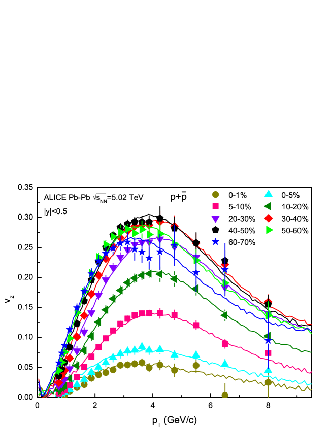
Figure 3: As for Fig. 1, but showing $v_{2}(p_{T})$ of $p+\bar{p}$ for a given centrality 24 .

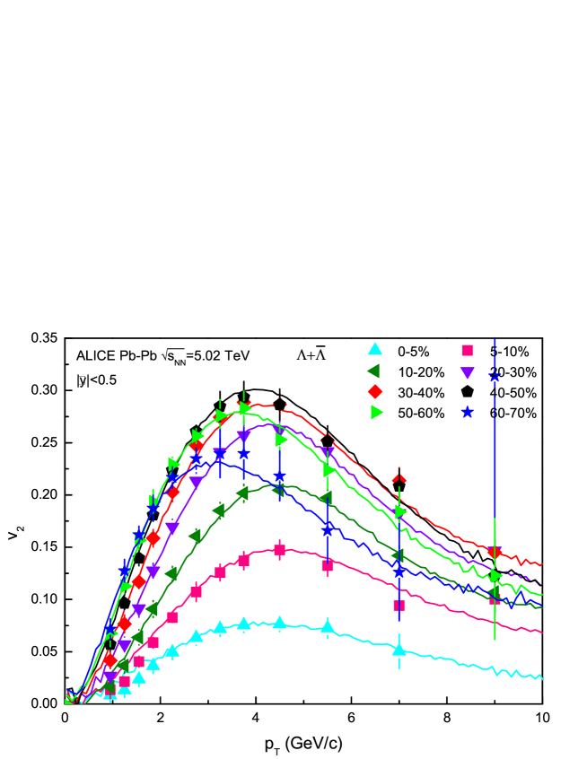
Figure 4: As for Fig. 1, but showing $v_{2}(p_{T})$ of $\Lambda+\bar{\Lambda}$ for a given centrality. 24

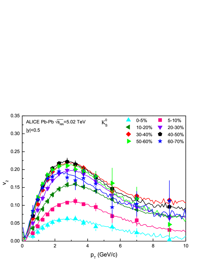
Figure 5: As for Fig. 1, but showing $v_{2}(p_{T})$ of $K_{s}^{0}$ for a given centrality. 24

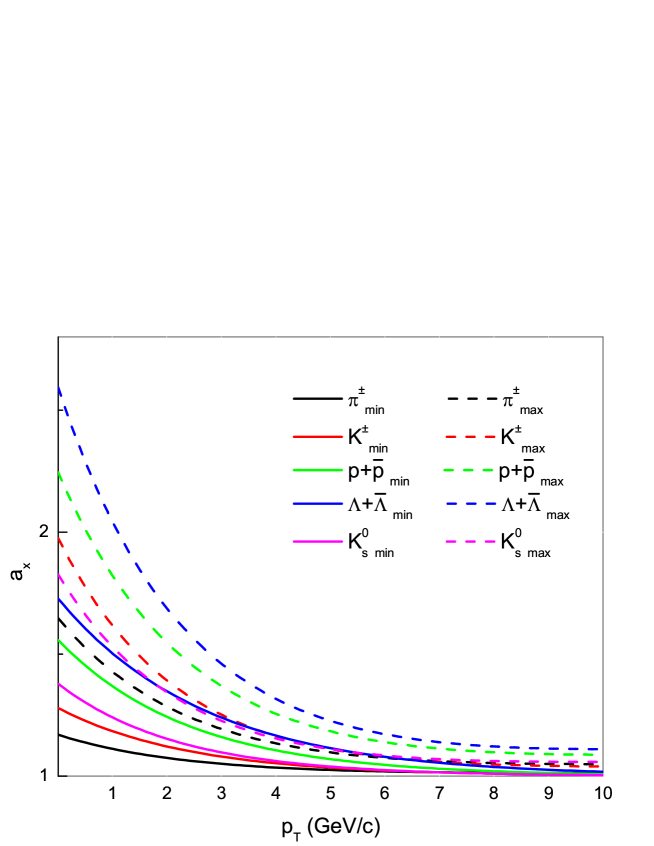
Figure 6: Transverse momentum dependency on the deformation parameter $a_{x}$ of $\pi^{\pm}$, $K^{\pm}$, $p+\bar{p}$, $\Lambda+\bar{\Lambda}$, and $K_{s}^{0}$. The curves are the results of this fitted based on Eq.(11).

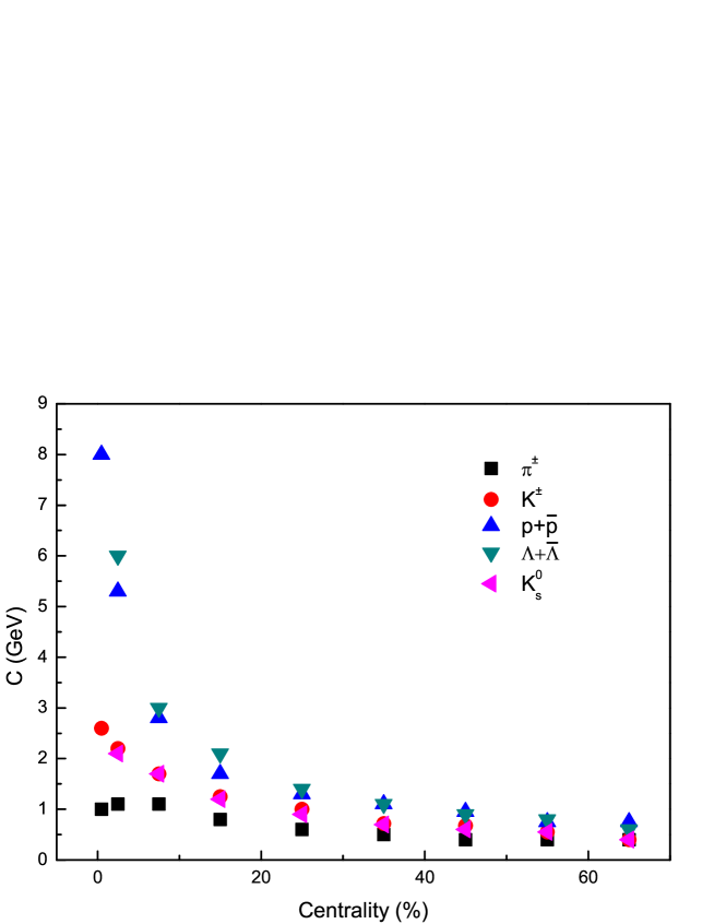
Figure 7: Free parameter $C$ dependency on the centrality classes.