Harnessing elasticity to generate self-oscillation via an electrohydrodynamic instability

Abstract

Under a steady DC electric field of sufficient strength, a weakly conducting dielectric sphere in a dielectric solvent with higher conductivity can undergo spontaneous spinning (Quincke rotation) through a pitchfork bifurcation. We design an object composed of a dielectric sphere and an elastic filament. By solving an elasto-electro-hydrodynamic (EEH) problem numerically, we uncover an EEH instability exhibiting diverse dynamic responses. Varying the bending stiffness of the filament, the composite object displays three behaviours: a stationary state, undulatory swimming and steady spinning, where the swimming results from a self-oscillatory instability through a Hopf bifurcation. By conducting a linear stability analysis incorporating an elastohydrodynamic model, we theoretically predict the growth rates and critical conditions, which agree well with the numerical counterparts. We also propose a reduced model system consisting of a minimal elastic structure which reproduces the EEH instability. The elasto-viscous response of the composite structure is able to transform the pitchfork bifurcation into a Hopf bifurcation, leading to self-oscillation. Our results imply a new way of harnessing elastic media to engineer self-oscillations, and more generally, to manipulate and diversify the bifurcations and the corresponding instabilities. These ideas will be useful in designing soft, environmentally adaptive machines.

March 17, 2024

1 Introduction

Active matter has been attracting much interest from a broad range of research communities (Ramaswamy, 2010; Cates & MacKintosh, 2011; Marchetti et al., 2013; Needleman & Dogic, 2017). At the micron scale, active matter consists of a large number of active agents that are able to convert energy to achieve directed or persistent motions, which include those of living microorganisms, synthetic micro-robots, biopolymers such as actin filaments, etc. The motions of these active agents are attributed to a wide range of mechanisms (Lauga & Powers, 2009; Marchetti et al., 2013; Alapan et al., 2019), e.g. one of the most common strategies adopted by natural and artificial micro-swimmers lies in the beating and wiggling of slender structures such as cilia and filaments, which are hair-like slender microscale structures that play an important role in various biological processes (Fawcett, 1961), such as swimming, pumping, mixing, cytoplasmic streaming, etc. The biological organelles deliver these functionalities by performing rhythmic, wave-like motions.

To achieve persistent motions, cyclic or oscillatory motions are needed, yet, the mechanism underlying the emergence of such oscillations remains unclear. Two major hypotheses, geometric feedback (Brokaw, 1971, 2009; Riedel-Kruse et al., 2007; Sartori et al., 2016; Hines & Blum, 1983; Hilfinger et al., 2009) and “flutter” or buckling instability (Bayly & Dutcher, 2016; De Canio et al., 2017; Ling et al., 2018; Hu & Bayly, 2018; Fatehiboroujeni et al., 2018), have been raised based on theory and/or simulations: the first hypothesis assumes that a time-dependent dynein activity (switching on/off or modulation) is necessary to trigger the oscillations; the second one suggests that a steady point force or force distributions acting along the axial direction of a flexible filament can trigger its oscillatory motion through a “flutter” or buckling instability. These forces are in fact called the “follower force” in the mechanics literature (Pflüger, 1950; Ziegler, 1952; Herrmann & Bungay, 1964). Because the follower force was initially invented theoretically and assumed to be always tangential to the slender structure regardless of its time-dependent deformation, it was demonstrated only mathematically and has been considered impractical (Koiter, 1996). However, it was recently realised experimentally on a metre-scale rod (Bigoni et al., 2018).

To drive the oscillations of artificial cilia and filaments of micron scale, different methods that exploit magnetic (Dreyfus et al., 2005; Singh et al., 2005; Evans et al., 2007; Livanovičs & Cēbers, 2012; Hanasoge et al., 2017; Huang et al., 2019) , electrostatic (den Toonder et al., 2008), piezoelectric (Kieseok et al., 2009), optical (van Oosten et al., 2009) and hydrogel-based actuations (Sidorenko et al., 2007; Masuda et al., 2013) have been developed. Nonetheless, these practises relied on a time-dependent power source, except for the self-oscillation of polymer brushes triggered by the Belousov-Zhabotinsky reaction (Masuda et al., 2013). This reaction-based beating shares with other biological processes, such as mammalian otoacoustic emissions (Gold, 1948; Kemp, 1979) and glycolysis (Sel’kov, 1968) the same feature: self-oscillation, that is generating and sustaining a periodic motion based on a power source without a corresponding periodicity (Jenkins, 2013).

In our recent work (Zhu & Stone, 2019), we proposed a chemical-reaction-free and follower-force-free strategy to engineer the self-oscillations of artificial structures by employing a time-independent, uniform electric field. We reported an elasto-electro-hydrodynamic (EEH) instability based on the Quincke rotation (QR) instability, and utilised it to drive various motions of an object composed of a dielectric spherical particle with an attached elastic filament. In this work, we will present in detail the setup and the mathematical description of the new EEH problem. First, we numerically solve the system coupling the electrohydrodynamics of the particle in a dielectric fluid and the elastohydrodynamics of the filament in a viscous fluid. We identify the emergence of the EEH instability that produces the self-oscillation of the composite object. The oscillations in turn cause the object to translate. Then, we perform a linear stability analysis (LSA) incorporating an elastohydrodynamic model to predict the onset of self-oscillatory instability. Finally, we propose a minimal model that can reproduce the similar EEH instability.

We describe the setup and governing equations of the EEH problem in § 2, and demonstrate the numerical results in § 3. The elastohydrodynamic model and LSA are shown in § 4, followed by § 5 illustrating the minimal model. Finally, we conclude our observations and provide some discussions in § 6.

2 Problem setup and mathematical formulations

We consider a weakly conducting dielectric spherical particle of radius $A$, which has attached an inextensible elastic filament of contour length $L$. The filament is cylindrical with a constant cross-section of radius $a$, and its slenderness is $\epsilon_{\mathrm{sl}}=a/L\ll 1$. We fix $\epsilon_{\mathrm{sl}}=0.01$ in this work. The composite object is subject to a time-independent uniform electric field $\mathbf{E}=E\mathbf{e}_{z}$ (see figure 1), where $\mathbf{e}_{z}$ is the $z$-direction basis vector of the laboratory coordinates system $\mathbf{e}_{xyz}$. The centreline of the filament is described by $\mathbf{r}\left(s,t\right)$, where $s$ indicates the arclength. The base J ($s=0$) of the filament is clamped at the particle surface, namely, the tangent vector $\partial\mathbf{r}/\partial s|_{s=0}=-\mathbf{e}_{\mathrm{p}}$ at the base always passes through the particle centre P, regardless of its deformation and the orientation vector $\mathbf{e}_{\mathrm{p}}$ of the particle. The size ratio between the particle and filament is $\alpha=A/L$. We consider only the bending deformation of the filament with a bending stiffness of $D=\pi a^{4}Y/4$, where $Y$ denotes Young’s modulus.

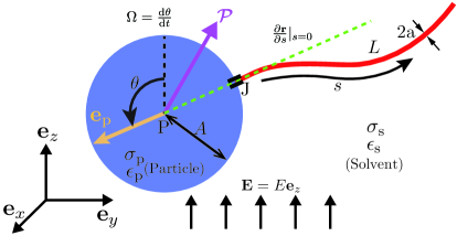
Figure 1: Schematic of the setup: a dielectric spherical particle of radius $A$ attached with a flexible filament of contour length $L$ is exposed to a steady uniform electrical field $\mathbf{E}=E\mathbf{e}_{z}$. The composite object’s motion, orientation $\mathbf{e}_{\mathrm{p}}$ and induced dipole $\mathbfcal{P}$ are all constrained to the $yz$-plane, and $\mathbf{e}_{\mathrm{p}}$ is described by the angle $\theta$ with respect to $\mathbf{e}_{z}$.

The composite object is immersed in a dielectric solvent fluid with dynamic viscosity $\mu$. The electrical conductivity and absolute permittivity of the solvent are $\sigma_{\mathrm{s}}$ and $\epsilon_{\mathrm{s}}$, respectively, and those of the particle are $\sigma_{\mathrm{p}}$ and $\epsilon_{\mathrm{p}}$; $R=\sigma_{\mathrm{p}}/\sigma_{\mathrm{s}}$ and $S=\epsilon_{\mathrm{p}}/\epsilon_{\mathrm{s}}$ indicate the ratios. The terms $\tau_{\mathrm{s}}=\epsilon_{\mathrm{s}}/\sigma_{\mathrm{s}}$ and $\tau_{\mathrm{p}}=\epsilon_{\mathrm{p}}/\sigma_{\mathrm{p}}$ denote the charge relaxation time of the solvent and particle, respectively. These electrical properties are important to the induced QR electrohydrodynamic instability that is critical to the dynamics in this paper. Their values are based on experiments (Brosseau et al., 2017), where $R=2.3\times 10^{-7}$ and $S=0.84$ are fixed in this work. Though the filament will also be polarised like the particle, the induced electric torque on the filament will be much weaker than that on the particle (see § 6 for a detailed discussion). We thus do not consider the electrohydrodynamics of the filament in this work.

2.1 Assumptions

The numerical simulations are carried out by invoking several assumptions. Motivated by biomimetic applications at the micron scale, we neglect the inertia of the fluid and particle. The fluid motion is therefore governed by the Stokes equations, and the particle satisfies instantaneous force- and torque-free conditions. The movement of the composite object is constrained to be planar, such that the particle centre P and filament position $\mathbf{r}(s,t)$ are in the $yz$-plane.

We adopt the local resistive-force theory (Batchelor, 1970) to calculate the hydrodynamic forces on the filament. We further ignore the hydrodynamic interactions between the particle and the filament. In the elastohydrodynamic model developed for LSA, we also assume that the filament undergoes weak deformation.

2.2 Electrohydrodynamics of the particle

When a dielectric particle in a dielectric solvent is exposed to an electric field, the interface of the particle will be polarised. The total induced dipole $\mathbfcal{P}^{\mathrm{total}}$ consists of an instantaneous part $\mathbfcal{P}^{\infty}$ and a retarding part $\mathbfcal{P}$, viz. $\mathbfcal{P}^{\mathrm{total}}=\mathbfcal{P}^{\infty}+\mathbfcal{P}$. Both vectors are defined by three components, $\mathcal{P}^{\infty}_{i}$ and $\mathcal{P}_{i}$ ($i=1...3$) in the reference frame $\mathbf{e}_{123}$ that rotates with the particle (see figure 2). For a homogeneous spherical particle, its Maxwell-Wagner polarisation time $\tau_{\mathrm{MW}}$, and low- and high-frequency susceptibilities, $\chi^{0}$ and $\chi^{\infty}$, respectively, are isotropic, hence the $i$-th component of the instantaneous dipole $\mathbfcal{P}^{\infty}$ is

$$\mathcal{P}^{\infty}_{i}=\chi^{\infty}E_{i}.$$ (1)

In the rotating reference frame of the particle, the retarding dipole $\mathbfcal{P}$ is governed by (Tsebers, 1980b; Cēbers et al., 2000)

$$\frac{\partial\mathcal{P}_{i}}{\partial t}=-\frac{1}{\tau_{\mathrm{MW}}}\left[\mathcal{P}_{i}-\left(\chi^{0}-\chi^{\infty}\right)E_{i}\right],$$ (2)

where

$$\kappa=\frac{R+2}{S+2}$$ (3)

and $\tau_{\mathrm{MW}}=\tau_{\mathrm{s}}/\kappa$. It is well known that when the charge relaxation time $\tau_{\mathrm{p}}$ of the particle is larger than that of the solvent $\tau_{\mathrm{s}}$, i.e., $R/S<1$, $\mathbfcal{P}$ is oriented opposite to the electric field. This directional misalignment is the necessary condition for the electro-rotation of the particle, the so-called Quincke rotation (Quincke, 1896), which occurs when, in addition, the strength $E$ of the electric field is above a critical value $E^{\mathrm{cri}}$ derived theoretically as (Jones, 1984; Brosseau et al., 2017) (see appendix B)

$$E^{\mathrm{cri}}=\sqrt{\frac{2\sigma_{\mathrm{s}}\mu(R+2)^{2}}{3\epsilon_{\mathrm{s}}^{2}(S-R)}}.$$ (4)

We do not consider the hydrodynamic interactions between the spherical particle and filament, hence the dynamics of the particle can be obtained by using its translational and rotational mobility factors. Assuming that the particle rotates at angular velocity $\boldsymbol{\Omega}$ about its centre P, which translates at velocity $\mathbf{U}$, the force and torque balances on the particle give

$$\mathbf{F}^{\mathrm{f}\rightarrow\mathrm{p}}-\beta_{\mathrm{drag}}\mathbf{U} =\mathbf{0},$$ (5a)

$$\boldsymbol{\Gamma}^{\mathrm{f}\rightarrow\mathrm{p}}+\boldsymbol{\Gamma}^{\mathrm{elec}}-\gamma_{\mathrm{drag}}\boldsymbol{\Omega} =\mathbf{0},$$ (5b)

where $\mathbf{F}^{\mathrm{f}\rightarrow\mathrm{p}}$ denotes the force exerted by the filament on the particle, $\boldsymbol{\Gamma}^{\mathrm{f}\rightarrow\mathrm{p}}$ the torque with respect to the particle centre P, and $\beta_{\mathrm{drag}}=6\pi\mu A$ and $\gamma_{\mathrm{drag}}=8\pi\mu A^{3}$ are the translational and rotational drag coefficients of a sphere in the creeping flow, respectively. Also, $\boldsymbol{\Gamma}^{\mathrm{elec}}$ is the electric torque on the particle with respect to its centre P, that is

$$\boldsymbol{\Gamma}^{\mathrm{elec}}=\mathbfcal{P}^{\mathrm{total}}\times\mathbf{E}=\mathbfcal{P}^{\infty}\times\mathbf{E}+\mathbfcal{P}\times\mathbf{E}=\mathbfcal{P}\times\mathbf{E},$$ (6)

where $\mathbfcal{P}^{\infty}\times\mathbf{E}\equiv\mathbf{0}$ for an isotropic sphere because $\mathcal{P}^{\infty}_{i}$ linearly scales with $E_{i}$ in each direction by the same factor $\chi^{\infty}$ (see equation (1)). It is worth noting that $\mathbfcal{P}^{\infty}\times\mathbf{E}\neq\mathbf{0}$ for ellipsoidal particles, where the factor $\chi^{\infty}$ is direction dependent (Cēbers et al., 2000; Brosseau et al., 2017). The translation of the particle is driven by the elastic force exerted by the filament, which is balanced by the viscous drag, while the rotational motion of the particle is determined by the balance between the elastic, electric and hydrodynamic torques.

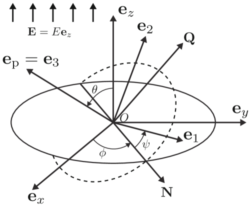
Figure 2: The reference frame $\mathbf{e}_{123}$ that rotates and translates with the particle, the orientation $\mathbf{e}_{\mathrm{p}}$ of the composite object coincides with $\mathbf{e}_{3}$. The proper Euler angles $[\theta,\phi,\psi]$ are adopted to describe the orientation $\mathbf{e}_{\mathrm{p}}$, where $\mathbf{N}$ denotes the nodal line direction and $\mathbf{Q}=\mathbf{e}_{3}\times\mathbf{N}$. We note that a graphical error occurred in a similar figure in our related work (Zhu & Stone, 2019), where $\psi$ ranges from $\mathbf{N}$ but erroneously to $\mathbf{e}_{y}$.

The orientation of the particle $\mathbf{e}_{\mathrm{p}}$ is defined as the direction from the filament base J towards the particle centre P, where $\mathbf{e}_{3}$ of the particle-based reference frame coincides with $\mathbf{e}_{\mathrm{p}}$. We have found it convenient to use the proper Euler angles $[\theta,\phi,\psi]$, see figure 2. Here, $\mathbfcal{P}$ is decomposed into $\mathbfcal{P}=\mathcal{P}_{3}\mathbf{e}_{3}+\mathcal{P}_{N}\mathbf{N}+\mathcal{P}_{Q}\mathbf{Q}$, where $\mathbf{N}$ indicates the nodal line direction and $\mathbf{Q}=\mathbf{e}_{3}\times\mathbf{N}$. This decomposition applies to other vectorial variables such as $\mathbf{E}$. We constrain $\mathbfcal{P}$ onto the $yz$-plane, hence $\phi=\psi\equiv 0$ and $\theta$ is the only angle indicating the orientation $\mathbf{e}_{\mathrm{p}}$; additionally, $\mathcal{P}_{N}=0$ and $\mathbf{e}_{x}=\mathbf{N}$. For the sake of completeness, we first derive the governing equations for a general situation without these constraints.

Using the torque-free condition equation (5b), we obtain the governing equations for $[\theta,\phi,\psi]$,

$$\frac{\partial\theta}{\partial t} =\frac{1}{\gamma_{\mathrm{d}}}\left(\Gamma^{\mathrm{f}\rightarrow\mathrm{p}}_{N}+E_{3}\mathcal{P}_{Q}-E_{Q}\mathcal{P}_{3}\right),$$ (7a)

$$\frac{\partial\phi}{\partial t} =\frac{1}{\gamma_{\mathrm{drag}}}\sin{\theta}\left(-E_{3}\mathcal{P}_{N}+\Gamma^{\mathrm{f}\rightarrow\mathrm{p}}_{Q}\right),$$ (7b)

$$\frac{\partial\psi}{\partial t} =\frac{1}{\gamma_{\mathrm{drag}}}\sin{\theta}\left(E\mathcal{P}_{N}-\Gamma^{\mathrm{f}\rightarrow\mathrm{p}}_{Q}\cos{\theta}\right),$$ (7c)

where $E_{3}=E\cos{\theta}$ and $E_{Q}=E\sin{\theta}$. The governing equations for $[\mathcal{P}_{N},\mathcal{P}_{Q},\mathcal{P}_{3}]$ are (Cēbers et al., 2000)

$$\frac{\partial\mathcal{P}_{N}}{\partial t}+\frac{\partial\psi}{\partial t}\mathcal{P}_{Q} =-\frac{1}{\tau_{\mathrm{MW}}}\mathcal{P}_{N},$$ (8a)

$$\frac{\partial\mathcal{P}_{Q}}{\partial t}-\frac{\partial\psi}{\partial t}\mathcal{P}_{N} =-\frac{1}{\tau_{\mathrm{MW}}}\left[\mathcal{P}_{Q}-\left(\chi^{0}-\chi^{\infty}\right)E_{Q}\right],$$ (8b)

$$\frac{\partial\mathcal{P}_{3}}{\partial t} =-\frac{1}{\tau_{\mathrm{MW}}}\left[\mathcal{P}_{3}-\left(\chi^{0}-\chi^{\infty}\right)E_{3}\right].$$ (8c)

We choose the charge relaxation time of the solvent $\tau_{\mathrm{s}}$ as the characteristic time, $L/\tau_{\mathrm{s}}$ the characteristic velocity, and $E^{\mathrm{cri}}$ and $D/(LE^{\mathrm{cri}})$ the characteristic strength of the electrical field and polarisation dipole, respectively. Using $\;\bar{}\;$ to indicate the dimensionless variables hereafter, the dimensionless equations for the Euler angles $[\theta,\phi,\psi]$ are

$$\frac{\partial\theta}{\partial\bar{t}} =\frac{1}{\bar{\eta}}\left(\bar{\Gamma}^{\mathrm{f}\rightarrow\mathrm{p}}_{N}+\bar{E}_{3}\bar{\mathcal{P}}_{Q}-\bar{E}_{Q}\bar{\mathcal{P}}_{3}\right),$$ (9a)

$$\frac{\partial\phi}{\partial\bar{t}} =\frac{1}{\bar{\eta}\sin{\theta}}\left(-\bar{E}_{3}\bar{\mathcal{P}}_{N}+\bar{\Gamma}^{\mathrm{f}\rightarrow\mathrm{p}}_{Q}\right),$$ (9b)

$$\frac{\partial\psi}{\partial\bar{t}} =\frac{1}{\bar{\eta}\sin{\theta}}\left(\bar{E}\bar{\mathcal{P}}_{N}-\bar{\Gamma}^{\mathrm{f}\rightarrow\mathrm{p}}_{Q}\cos{\theta}\right),$$ (9c)

as derived in Cēbers et al. (2000) in the absence of the elastic torque $\bar{\boldsymbol{\Gamma}}^{\mathrm{f}\rightarrow\mathrm{p}}$. Here,

$$\bar{\eta}=\alpha^{3}\bar{\mu},$$ (10)

with

$$\bar{\mu}=\frac{8\pi\mu L^{4}}{D\tau_{\mathrm{s}}}$$ (11)

defined as the elasto-electro-viscous (EEV) parameter. The dimensionless governing equations for $[\bar{\mathcal{P}}_{N},\bar{\mathcal{P}}_{Q},\bar{\mathcal{P}}_{3}]$ following from equation (8) are

$$\frac{\partial\bar{\mathcal{P}}_{N}}{\partial\bar{t}} =-\kappa\bar{\mathcal{P}}_{N}-\frac{\partial\psi}{\partial\bar{t}}\bar{\mathcal{P}}_{Q},$$ (12a)

$$\frac{\partial\bar{\mathcal{P}}_{Q}}{\partial\bar{t}} =-\kappa\left(\bar{\mathcal{P}}_{Q}+\kappa\bar{\eta}\bar{E}_{Q}\right)+\frac{\partial\psi}{\partial t}\bar{\mathcal{P}}_{N},$$ (12b)

$$\frac{\partial\bar{\mathcal{P}}_{3}}{\partial\bar{t}} =-\kappa\left(\bar{\mathcal{P}}_{3}+\kappa\bar{\eta}\bar{E}_{3}\right),$$ (12c)

where $\kappa=(R+2)/(S+2)$ as defined in equation (3). We slightly perturb the instantaneous polarisation $\bar{\mathbfcal{P}}^{\infty}$ and use it as the initial value $\bar{\mathbfcal{P}}_{\mathrm{ini}}$ of $\bar{\mathbfcal{P}}$, where

$$\bar{\mathbfcal{P}}^{\infty} =\frac{\bar{\eta}\kappa^{2}\bar{E}}{\kappa-(R-1)/(S-1)}\left(\mathbf{e}_{Q}\sin\theta+\mathbf{e}_{3}\cos\theta\right),$$ (13a)

$$\bar{\mathbfcal{P}}_{\mathrm{ini}} =\bar{\mathbfcal{P}}^{\infty}+\epsilon_{\mathcal{P}}|\bar{\mathbfcal{P}}^{\infty}|,$$ (13b)

with $\epsilon_{\mathcal{P}}=\mathcal{O}(10^{-4})-\mathcal{O}(10^{-3})$.

The dimensionless force- and torque-free conditions are

$$\bar{\mathbf{F}}^{\mathrm{f}\rightarrow\mathrm{p}}-3\alpha\bar{\mu}\bar{\mathbf{U}}/4 =\mathbf{0},$$ (14a)

$$\bar{\boldsymbol{\Gamma}}^{\mathrm{f}\rightarrow\mathrm{p}}+\bar{\mathbfcal{P}}\times\bar{\mathbf{E}}-\bar{\eta}\bar{\boldsymbol{\Omega}} =\mathbf{0}.$$ (14b)

Since we constrain the motion of the composite object and the induced dipole $\bar{\mathbfcal{P}}$ to the $yz$-plane, we solve equations (9a), (12b) and (12c) for $\theta$, $\bar{\mathcal{P}}_{Q}$ and $\bar{\mathcal{P}}_{3}$, where the last term $\frac{\partial\psi}{\partial t}\bar{\mathcal{P}}_{N}$ in equation (12b) vanishes.

2.3 Elastohydrodynamics of the filament

We describe here the elastohydrodynamic equations for the filament. By employing the slender body theory (SBT) considering the leading-order local drag (Batchelor, 1970), the relation between the velocity $\mathbf{r}_{t}$ of the filament centreline and the force per unit length exerted by the fluid onto the filament $\mathbf{f}(s,t)$ is

$$8\pi\mu\left(\mathbf{r}_{t}-\mathbf{U}^{\infty}\right)=c\left(\mathbf{I}+\mathbf{r}_{s}\mathbf{r}_{s}\right)\cdot\mathbf{f},$$ (15)

where $\mathbf{U}^{\infty}$ is the underlying flow velocity (background or imposed flow velocity) at $\mathbf{r}(s,t)$ and $\mathbf{U}^{\infty}=\mathbf{0}$ in this work; the subscripts $t$ and $s$ denote the partial derivatives with respect to $t$ and $s$, respectively and

$$c=1+2\log{\epsilon_{\mathrm{sl}}}<0.$$ (16)

The filament is assumed to be described by the Euler–Bernoulli constitutive law, and because the elastic force balances the hydrodynamic force anywhere on the centreline, we obtain

$$\mathbf{f}(s)=-\left(T(s)\mathbf{r}_{s}\right)_{s}+D\mathbf{r}_{ssss},$$ (17)

where $T(s,t)$ denotes the line tension, which acts as a Lagrangian multiplier to guarantee the inextensibility of the filament, i.e., $\mathbf{r}_{s}\cdot\mathbf{r}_{s}\equiv 1$.

By substituting equation (17) into equation (15), and choosing $L$ and $D/L^{2}$ as the characteristic length and force, respectively, we obtain the dimensionless equations for $\bar{\mathbf{r}}(\bar{s},\bar{t})$,

$$\bar{\mu}\bar{\mathbf{r}}_{\bar{t}}=-2c\bar{T}_{\bar{s}}\bar{\mathbf{r}}_{\bar{s}}-c\bar{T}\bar{\mathbf{r}}_{\bar{s}\bar{s}}+c\bar{\mathbf{r}}_{\bar{s}\bar{s}\bar{s}\bar{s}}+c\left(\bar{\mathbf{r}}_{\bar{s}}\cdot\bar{\mathbf{r}}_{\bar{s}\bar{s}\bar{s}\bar{s}}\right)\bar{\mathbf{r}}_{\bar{s}}.$$ (18)

The dimensionless equation for $\bar{T}\left(\bar{s}\right)$ reads,

$$2c\bar{T}_{\bar{s}\bar{s}}-c\bar{T}\bar{\mathbf{r}}_{\bar{s}\bar{s}}\cdot\bar{\mathbf{r}}_{\bar{s}\bar{s}}=-7c\bar{\mathbf{r}}_{\bar{s}\bar{s}}\cdot\bar{\mathbf{r}}_{\bar{s}\bar{s}\bar{s}\bar{s}}-6c\bar{\mathbf{r}}_{\bar{s}\bar{s}\bar{s}}\cdot\bar{\mathbf{r}}_{\bar{s}\bar{s}\bar{s}}-\bar{\mu}\beta_{\mathrm{p}}\left(1-\bar{\mathbf{r}}_{\bar{s}}\cdot\bar{\mathbf{r}}_{\bar{s}}\right),$$ (19)

where the last term on the right-hand side $-\bar{\mu}\beta_{\mathrm{p}}\left(1-\bar{\mathbf{r}}_{\bar{s}}\cdot\bar{\mathbf{r}}_{\bar{s}}\right)$ is an extra (numerical) penalisation term introduced (Tornberg & Shelley, 2004; Li et al., 2013) to preserve the local inextensibility constraint $\bar{\mathbf{r}}_{\bar{s}}\cdot\bar{\mathbf{r}}_{\bar{s}}\equiv 1$; $\beta_{\mathrm{p}}=100$ is adopted in our simulations. The boundary conditions (BCs) for $\bar{\mathbf{r}}(\bar{s},\bar{t})$ and $\bar{T}(\bar{s},\bar{t})$ at the free end $\bar{s}=1$ are

$$\bar{\mathbf{r}}_{\bar{s}\bar{s}} =\bar{\mathbf{r}}_{\bar{s}\bar{s}\bar{s}}=\mathbf{0},$$ (20a)

$$\bar{T} =0.$$ (20b)

The BCs at the clamped end $\bar{s}=0$ couple the elastohydrodynamics and electrohydrodynamics, as will be described next.

2.4 Elasto-electro-hydrodynamic coupling

The electrohydrodynamics of the dielectric particle in a dielectric solvent and the elastohydrodynamics of the flexible filament in a viscous fluid are coupled via, first the BCs of $\bar{\mathbf{r}}(\bar{s},\bar{t})$ and $\bar{T}(\bar{s},\bar{t})$ at the filament base $\bar{s}=0$, and second the elastic force $\bar{\mathbf{F}}^{\mathrm{f}\rightarrow\mathrm{p}}(\bar{t})$ and torque $\bar{\boldsymbol{\Gamma}}^{\mathrm{f}\rightarrow\mathrm{p}}(\bar{t})$ exerted by the filament on the particle (equation (14).

The BCs at the filament base $\bar{s}=0$ are

$$\bar{\mathbf{r}} =\bar{\mathbf{x}}_{\mathrm{p}}+\alpha\bar{\mathbf{r}}_{\bar{s}},$$ (21a)

$$\bar{\mathbf{r}}_{\bar{s}} =-\mathbf{e}_{\mathrm{p}},$$ (21b)

where $\bar{\mathbf{x}}_{\mathrm{p}}(\bar{t})$ denotes the dimensionless position of the particle centre P. Equations (21a) and  (21b) imply, respectively, that the filament base $\bar{s}=0$ is exactly on the particle surface, and the filament tangent vector at $\bar{s}=0$ always passes through the particle centre. Moreover, $\bar{\mathbf{x}}_{\mathrm{p}}(\bar{t})$ and $\mathbf{e}_{\mathrm{p}}(\bar{t})$ are connected to the particle kinematics through

$$\frac{\mathrm{d}\bar{\mathbf{x}}_{\mathrm{p}}}{\mathrm{d}\bar{t}} =\bar{\mathbf{U}},$$ (22a)

$$\frac{\mathrm{d}\mathbf{e}_{\mathrm{p}}}{\mathrm{d}\bar{t}} =\bar{\boldsymbol{\Omega}}\times\mathbf{e}_{\mathrm{p}},$$ (22b)

where $\bar{\mathbf{U}}(\bar{t})$ is linked to equation (14a) and $\bar{\boldsymbol{\Omega}}(\bar{t})$ to equation (9). The coupling is completed by the computation of $\bar{\mathbf{F}}^{\mathrm{f}\rightarrow\mathrm{p}}$ and $\bar{\boldsymbol{\Gamma}}^{\mathrm{f}\rightarrow\mathrm{p}}$,

$$\bar{\mathbf{F}}^{\mathrm{f}\rightarrow\mathrm{p}} =\left[-\bar{\mathbf{r}}_{\bar{s}\bar{s}\bar{s}}+\bar{T}\bar{\mathbf{r}}_{\bar{s}}\right]|_{\bar{s}=0},$$ (23a)

$$\bar{\boldsymbol{\Gamma}}^{\mathrm{f}\rightarrow\mathrm{p}} =\left[\bar{\mathbf{r}}_{\bar{s}}\times\left(\bar{\mathbf{r}}_{\bar{s}\bar{s}}-\alpha\bar{\mathbf{r}}_{\bar{s}\bar{s}\bar{s}}\right)\right]|_{\bar{s}=0}.$$ (23b)

For completeness, we write the BC for the tension $\bar{T}$ at the filament base $\bar{s}=0$

$$2c\bar{T}_{\bar{s}}+6c\bar{\mathbf{r}}_{\bar{s}\bar{s}}\cdot\bar{\mathbf{r}}_{\bar{s}\bar{s}\bar{s}}=-\bar{\mu}\bar{\mathbf{r}}_{\bar{s}}\cdot\bar{\mathbf{r}}_{\bar{t}}.$$ (24)

3 Numerical results

In the original QR phenomenon (without a filament), the particle rotates when the dimensionless electric field is above $1$, namely, $\bar{E}\geq 1$. We hereby investigate the influence of the bending stiffness of the filament by varying $\bar{\mu}$, where we fix the electric field $\bar{E}=1.5$ at which an individual particle undergoes steady QR. We fix the size ratio $\alpha=0.3$ in this section.

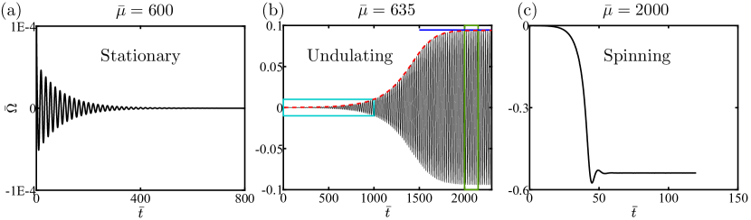
Figure 3: $\bar{\mu}$-dependent time evolution of the rotational velocity $\bar{\Omega}\left(\bar{t}\right)$ for (a) $\bar{\mu}=600$, (b) $\bar{\mu}=635$ and (c) $\bar{\mu}=2000$ when $\bar{E}=1.5$. Their corresponding equilibrium configurations are stationary, undulating and steady spinning, respectively. Note that $\bar{\Omega}_{\bar{t}=0}$ is not necessarily zero because the induced dipole $\bar{\mathbfcal{P}}$ is slightly perturbed at $\bar{t}=0$, see equation (13); moreover, (a) and (b) have strikingly different scales for $\bar{\Omega}$.

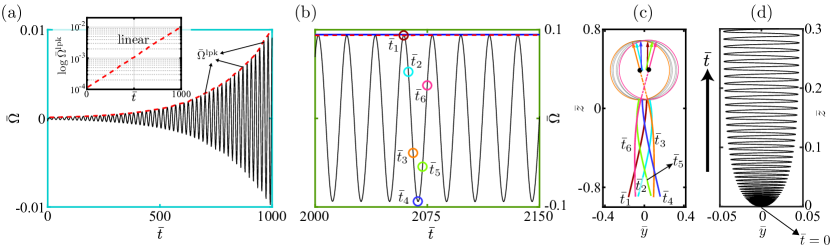
Figure 4: (a) Highlighted cyan domain of figure 3b indicating the initial rapidly growing period of $\bar{\Omega}(t^{\ast})$, for $\bar{\mu}=635$ and $\bar{E}=1.5$. The red curve denotes the local peak $\bar{\Omega}^{\mathrm{lpk}}$, and the inset of (a) shows the linear dependence of $\log{\bar{\Omega}^{\mathrm{lpk}}}$ on $\bar{t}$. (b) Highlighted green domain of figure 3b corresponding to the time-periodic response of $\bar{\Omega}(t^{\ast})$, where consecutive time instants $\bar{t}_{i}$ ($i=1,...,6$) within a period are marked. (c) Particle-filament configurations at $\bar{t}_{i}$. (d) Trajectory of the particle centre within $\bar{t}\in[0,1940]$.

We observe that the composite object exhibits three $\bar{\mu}$-dependent scenarios, indicated by the time evolution of the rotational velocity $\bar{\Omega}$ shown in figure 3. When $\bar{\mu}=600$ (figure 3a), $\bar{\Omega}$ decays dramatically and eventually becomes zero, indicating that the object relaxes to a stationary state. Increasing $\bar{\mu}$ to $635$ (figure 3b), the time evolution of $\bar{\Omega}$ features two phases: in the initial phase (cyan domain), it grows rapidly due to self-oscillation; in the second phase (green domain), it reaches a time-periodic state with a constant amplitude of approximately $0.1$. The third type of response is illustrated by $\bar{\mu}=2000$, where $\bar{\Omega}$ eventually approaches a steady value around $-0.6$.

We further scrutinise the $\bar{\mu}=635$ case. The close-up views of the initially rapidly growing phase (cyan domain) and saturated time-periodic phase (green domain) are shown in figure 4a and b, respectively. The red curve connecting the local peaks $\bar{\Omega}^{\mathrm{lpk}}$ of $\bar{\Omega}$ implies an exponential growth of $\bar{\Omega}$ in time. This trend is confirmed by the linear relationship between $\log{\bar{\Omega}^{\mathrm{lpk}}}$ and $\bar{t}$ shown in the inset of figure 4a. The time-periodic phase enlarged in figure 4b reveals its sinusoidal-like variation characterised by fore-aft temporal symmetry. Six times within one period of this phase are marked, with their corresponding positions and orientations of the particle, and the profiles of the filament depicted in figure 4c. The oscillating particle drives the filament to wiggle, because the filament is clamped onto the particle. The wiggling filament provides thrust to the whole object, as a natural resemblance to a biological appendage. Consequently, the object achieves locomotion, following a wave-like trajectory (figure 4d). The wavy path is tightly packed near $\bar{t}=0$, implying the slow motion of the object undergoing small-amplitude oscillation in the initial phase.

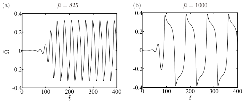
Figure 5: Time evolution of the rotational velocity $\bar{\Omega}\left(\bar{t}\right)$ when $\bar{E}=1.5$ for (a) $\bar{\mu}=825$ and (b) $\bar{\mu}=1000$.

We observe that when $\bar{\mu}$ lies in the self-oscillating regime, the time evolution of $\bar{\Omega}$ varies with $\bar{\mu}$. As shown in figure 5 for $\bar{\mu}=825$ and $1000$, for a larger $\bar{\mu}$ it takes fewer time periods for the perturbation to reach its time-periodic state. In addition, that state clearly breaks fore-aft symmetry with increasing $\bar{\mu}$.

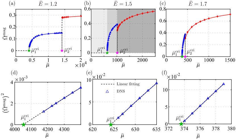
Figure 6: Amplitude $\bar{\Omega}^{\mathrm{mag}}$ of the rotational velocity as a function $\bar{\mu}$ for (a) $\bar{E}=1.2$, (b) $1.5$ and (c) $1.7$. The three $\bar{\mu}$-dependent regimes, stationary (dashed lines), undulating (triangles) and steady spinning (diamonds) of the composite object are separated by two thresholds $\bar{\mu}_{1}^{\mathrm{cri}}$ and $\bar{\mu}_{2}^{\mathrm{cri}}$. (d), (e) and (f) show the linear variation of $\left(\bar{\Omega}^{\mathrm{mag}}\right)^{2}$ in $\bar{\mu}$ in close proximity to $\bar{\mu}_{1}^{\mathrm{cri}}$ for $\bar{E}=1.2$, $1.5$ and $1.7$, respectively.

We next investigate the critical $\bar{\mu}$ values that separate the three regimes corresponding to the stationary, undulating and steady spinning states. Figure 6 displays the rotational velocity magnitude $\bar{\Omega}^{\mathrm{mag}}$ versus $\bar{\mu}$ for $\bar{E}=1.2$ (a), $1.5$ (b) and $1.7$ (c). When $\bar{\mu}\leq\bar{\mu}_{1}^{\mathrm{cri}}$, $\bar{\Omega}^{\mathrm{mag}}=0$ represents the fixed-point solution; when $\bar{\mu}\geq\bar{\mu}_{1}^{\mathrm{cri}}$, the non-zero $\bar{\Omega}^{\mathrm{mag}}$ representing the constant spinning speed corresponds to the asymmetric fixed-point solution; when $\bar{\mu}\in\left(\bar{\mu}_{1}^{\mathrm{cri}},\bar{\mu}_{2}^{\mathrm{cri}}\right)$, $\bar{\Omega}^{\mathrm{mag}}$ indicates the magnitude of the oscillating $\bar{\Omega}$ when it reaches a time-periodic state. We plot $\left(\bar{\Omega}^{\mathrm{mag}}\right)^{2}$ as a function of $\bar{\mu}$ in close proximity to $\bar{\mu}_{1}^{\mathrm{cri}}$ in figure 6d-f. The linear dependence of $\left(\bar{\Omega}^{\mathrm{mag}}\right)^{2}$ on $\bar{\mu}$ implies that the instability occurs at $\bar{\mu}_{1}^{\mathrm{cri}}$ through a Hopf bifurcation from where a limit-cycle solution emerges. Moreover, the $\bar{\Omega}^{\mathrm{mag}}(\bar{\mu})$ profile also indicates the supercritical nature of the Hopf bifurcation. On the other hand, a sudden jump of $\bar{\Omega}^{\mathrm{mag}}$ at $\bar{\mu}_{2}^{\mathrm{cri}}$ signifies a secondary bifurcation where the limit cycle shrinks to a fixed point or vice versa.

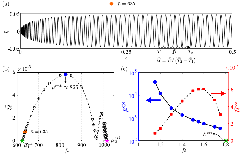
Figure 7: (a) Trajectory of the particle centre for $\bar{\mu}=635$, when $\bar{E}=1.5$. The dashed arrow indicates how the effective translational velocity $\bar{\mathcal{U}}$ is quantified. (b) $\bar{\mathcal{U}}$ versus $\bar{\mu}\in\left(\bar{\mu}_{1}^{\mathrm{cri}},\bar{\mu}_{2}^{\mathrm{cri}}\right)$ when $\bar{E}=1.5$, $\bar{\mathcal{U}}$ reaches an optimal value $\bar{\mathcal{U}}^{\mathrm{opt}}\approx 6\times 10^{-3}$ at $\bar{\mu}=\bar{\mu}^{\mathrm{opt}}\approx 825$. (c) The optimal EEV number $\bar{\mu}^{\mathrm{opt}}$ when the composite object attains the maximum effective translational velocity $\bar{\mathcal{U}}^{\mathrm{opt}}$; $\bar{\mu}^{\mathrm{opt}}$ and $\bar{\mathcal{U}}^{\mathrm{opt}}$ are plotted versus the field strength $\bar{E}$.

Having demonstrated that the composite object is able to achieve propulsion by self-oscillatory undulation, we naturally examine its propulsive performance. Shown in figure 7a, when the undulating swimmer reaches its time-periodic state, its trajectory resembles a periodic wave propagating along a straight direction (dashed arrow). We thus define the effective translational velocity $\bar{\mathcal{U}}$ of the swimmer as the propagation speed of the wave, that is $\bar{\mathcal{U}}=\bar{\mathcal{D}}/\left(\bar{T}_{2}-\bar{T}_{1}\right)$. This effective velocity $\bar{\mathcal{U}}$ exhibits a clear non-monotonic variation in $\bar{\mu}$; it reaches its maximum value at an optimal EEV number $\bar{\mu}=\bar{\mu}^{\mathrm{opt}}\approx 825$ and becomes zero when $\bar{\mu}\rightarrow\bar{\mu}_{1}^{\mathrm{cri}}$ and $\bar{\mu}\rightarrow\bar{\mu}_{2}^{\mathrm{cri}}$. Such a non-monotonic trend is expected, since when $\bar{\mu}$ is outside the self-oscillating regime $[\bar{\mu}_{1}^{\mathrm{cri}},\bar{\mu}_{2}^{\mathrm{cri}}]$, the object either remains stationary or spins steadily, resulting in no net locomotion. It is also worth noting that $\bar{\mathcal{U}}$ exhibits wavy variation near $\bar{\mu}_{2}^{\mathrm{cri}}$. In this regime, the filament is so deflected and the hydrodynamic interactions between the particle and filament can be reasonably strong due to the decreasing distance between them. Since our simulations do not consider the hydrodynamic interactions, hence it is not self-consistent to interrogate the data in detail in this regime.

Finally, we show in figure 7c the dependence of the optimal swimming condition, $\bar{\mu}^{\mathrm{opt}}$ and $\bar{\mathcal{U}}^{\mathrm{opt}}$, on the electric field strength $\bar{E}$. The optimal EEV number $\bar{\mu}^{\mathrm{opt}}$ decreases with $\bar{E}$ monotonically; in contrast, the optimal velocity $\bar{\mathcal{U}}^{\mathrm{opt}}$ displays a non-monotonic variation in $\bar{E}$, reaching a maximum value of approximately $6\times 10^{-3}$ at $\bar{E}\approx 1.55-1.6$. This non-monotonic trend is not surprising. In fact, self-oscillation of the composite object only emerges when $1<\bar{E}<\bar{\mathcal{E}}^{\mathrm{cri}}$, where $\bar{\mathcal{E}}^{\mathrm{cri}}$ represents the critical electric field above which the particle jointed with a rigid rod ($\bar{\mu}\rightarrow 0$) of the same length and slenderness will undergo the QR instability. Hence, when $\bar{E}\geq\bar{\mathcal{E}}^{\mathrm{cri}}$, the composite object will spin steadily but not self-propel regardless of the filament rigidity. On the other hand, when $\bar{E}\leq 1$, the extra anchored filament will further stabilise the original QR particle, hence the composite object will be stationary. We further note that the optimal translational velocity $\approx 6\times 10^{-3}$ is in the range $\left(1,15\right)\times 10^{-3}$ of the dimensionless speed of a magnetically driven flexible artificial flagellum (Dreyfus et al., 2005).

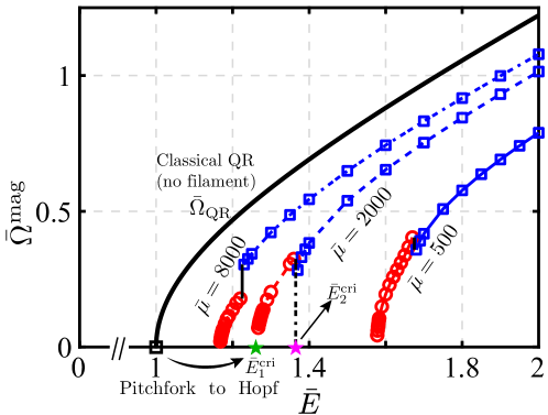
Figure 8: Amplitude $\bar{\Omega}^{\mathrm{mag}}$ of the rotational velocity versus $\bar{E}$ for three EEV numbers $\bar{\mu}=500$, $2000$ and $8000$. $\bar{E}_{1}^{\mathrm{cri}}$ (green star) and $\bar{E}_{2}^{\mathrm{cri}}$ (magenta star) indicate where the Hopf and secondary bifurcations occur, respectively. The solid curve corresponds to the original QR rotational velocity, $\bar{\Omega}_{\mathrm{QR}}$ (see equation (73)) and the hollow square denotes $\bar{E}=1$, the occurrence of the pitchfork bifurcation.

By analogy to the results in figure 6a-c, we show in figure 8 $\bar{\Omega}^{\mathrm{mag}}$ versus $\bar{E}$ as the bifurcation parameter for three EEV numbers $\bar{\mu}=500$, $2000$ and $8000$. A similar bifurcation diagram is identified: increasing $\bar{E}$ from zero, the stationary fixed point solution transits to a limit-cycle solution through a supercritical Hopf bifurcation at $\bar{E}_{1}^{\mathrm{cri}}$ (green star); that solution then jumps to a second fixed point solution (steady spinning) via a secondary bifurcation at $\bar{E}_{2}^{\mathrm{cri}}$ (magenta star). The original QR instability emerges at $\bar{E}=1$ (hollow square) through a supercritical pitchfork bifurcation (Turcu, 1987; Peters et al., 2005; Das & Saintillan, 2013). The filament manages to transform that bifurcation for an individual particle into a corresponding Hopf bifurcation leading to self-oscillation. It is not surprising that by increasing $\bar{\mu}$, the variation of $\bar{\Omega}^{\mathrm{mag}}$ for the composite object tends to recover that of the original QR corresponding to $\bar{\mu}\rightarrow\infty$.

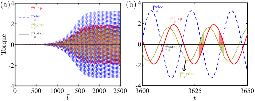
Figure 9: (a) Time evolution of the elastic $\bar{\Gamma}_{x}^{\mathrm{f}\rightarrow\mathrm{p}}$ (solid), electric $\bar{\Gamma}_{x}^{\mathrm{elec}}$ (dashed), hydrodynamic $\bar{\Gamma}_{x}^{\mathrm{hydro}}$ (dot-dashed) and total $\bar{\Gamma}_{x}^{\mathrm{total}}$ (straight solid) torque ($x$-component) on the particle with respect to its centre, where $\bar{\mu}=635$ and $\bar{E}=1.5$. (b) Close-up view of the time-periodic state. Shaded regions indicate when the elastic $\bar{\Gamma}_{x}^{\mathrm{f}\rightarrow\mathrm{p}}$ and hydrodynamic $\bar{\Gamma}_{x}^{\mathrm{hydro}}$ torques have opposite signs.

It is evident that the elastic torque $\bar{\boldsymbol{\Gamma}}^{\mathrm{f}\rightarrow\mathrm{p}}$ plays an important role in the torque balance. We examine the time evolution of the $x$-component of the torques, namely the elastic $\bar{\Gamma}_{x}^{\mathrm{f}\rightarrow\mathrm{p}}$, hydrodynamic $\bar{\Gamma}_{x}^{\mathrm{hydro}}$ and electric $\bar{\Gamma}_{x}^{\mathrm{hydro}}$ torques in figure 9 when $\bar{\mu}=635$ and $\bar{E}=1.5$. The sum of the torques $\bar{\Gamma}_{x}^{\mathrm{total}}=\bar{\Gamma}_{x}^{\mathrm{f}\rightarrow\mathrm{p}}+\bar{\Gamma}_{x}^{\mathrm{hydro}}+\bar{\Gamma}_{x}^{\mathrm{elec}}=0$ implies that the torque balance is well satisfied numerically. Similar to the evolution of the rotational velocity, the torques exhibit exponential growth in the initial phase before approaching a time-periodic state. The torque balance in this state is further scrutinised in figure 9b. Realising the negative relation between $\bar{\Gamma}^{\mathrm{hydro}}_{x}$ and $\bar{\Omega}$, we notice that $\bar{\Gamma}^{\mathrm{f}\rightarrow\mathrm{p}}_{x}$ and $\bar{\Omega}$ have the same sign in the two highlighted periods emphasising when the elastic $\bar{\Gamma}^{\mathrm{f}\rightarrow\mathrm{p}}_{x}$ and $\bar{\Gamma}^{\mathrm{hydro}}_{x}$ hydrodynamic torque contributions have opposite signs. The in-phase behaviour of $\bar{\Gamma}^{\mathrm{f}\rightarrow\mathrm{p}}_{x}$ and $\bar{\Omega}$ is a clear signature of negative damping, or positive feedback that triggers the linear instability of self-oscillation (Jenkins, 2013).

4 Linear stability analysis

4.1 Linearisation about the stationary equilibrium state

We perform LSA about the stationary equilibrium state of the composite particle when the filament is undeformed. In this section, we drop the bars for all of the dimensionless unknown variables (those over dimensionless parameters remain), unless otherwise specified. We linearise the governing equations of the particle orientation $\theta$, and the dipole components $[\mathcal{P}_{Q},\mathcal{P}_{3}]$. By incorporating into the LSA a theoretical model of the elasto-viscous response of the filament, we do not linearise the equations for the filament position $\mathbf{r}(s)$ and tension $T(s)$ as conducted in Guglielmini et al. (2012).

The state variables $[\theta,\mathcal{P}_{Q},\mathcal{P}_{3}]$ are decomposed into a base (equilibrium) state $[\hat{\theta},\hat{\mathcal{P}}_{Q},\hat{\mathcal{P}}_{3}]$ and a perturbation state $[\theta^{\prime},\mathcal{P}^{\prime}_{Q},\mathcal{P}^{\prime}_{3}]$, which satisfy

$$\theta =\hat{\theta}+\theta^{\prime},$$ (25a)

$$\mathcal{P}_{Q} =\hat{\mathcal{P}}_{Q}+\mathcal{P}^{\prime}_{Q},$$ (25b)

$$\mathcal{P}_{3} =\hat{\mathcal{P}}_{3}+\mathcal{P}^{\prime}_{3}.$$ (25c)

The perturbation-state variables $[\theta^{\prime},\mathcal{P}^{\prime}_{Q},\mathcal{P}^{\prime}_{3}]$ are assumed to be infinitesimal in LSA.

By substituting $\boldsymbol{\Gamma}^{\mathrm{f}\rightarrow\mathrm{p}}=\mathbf{0}$ and $\frac{\partial}{\partial t}=0$ into equations (9a), (12b) and 12c, we obtain the base-state dipoles

$$\hat{\mathcal{P}}_{Q} =-\kappa\bar{\eta}\bar{E}\sin{\hat{\theta}},$$ (26a)

$$\hat{\mathcal{P}}_{3} =-\kappa\bar{\eta}\bar{E}\cos{\hat{\theta}}.$$ (26b)

By substituting equations (25) and (26) into equations (9a), (12b) and (12c), and assuming small $\theta^{\prime}$, we derive the governing equations for the perturbation-state variables $[\theta^{\prime},\mathcal{P}^{\prime}_{Q},\mathcal{P}^{\prime}_{3}]$,

$$\frac{\partial\mathcal{P}^{\prime}_{Q}}{\partial t} =-\kappa\left(\mathcal{P}^{\prime}_{Q}+\kappa\bar{\eta}\bar{E}\theta^{\prime}\cos{\hat{\theta}}\right),$$ (27a)

$$\frac{\partial\mathcal{P}^{\prime}_{3}}{\partial t} =-\kappa\left(\mathcal{P}^{\prime}_{3}-\kappa\bar{\eta}\bar{E}\theta^{\prime}\sin{\hat{\theta}}\right),$$ (27b)

$$\frac{\partial\theta^{\prime}}{\partial t} =\frac{1}{\bar{\eta}}\left[\Gamma^{\mathrm{f}\rightarrow\mathrm{p}}_{N}+\bar{E}\left(\mathcal{P}^{\prime}_{Q}\cos{\hat{\theta}}-\mathcal{P}^{\prime}_{3}\sin{\hat{\theta}}+\kappa\bar{\eta}\bar{E}\theta^{\prime}\right)\right].$$ (27c)

Adopting the normal-mode approach, we assume that the perturbations vary exponentially in time with a complex rate $\sigma=\sigma_{r}+\mathrm{i}\sigma_{i}$, so $\left[\mathcal{P}^{\prime}_{Q},\mathcal{P}^{\prime}_{3},\theta^{\prime}\right]=\left[\Phi,\Pi,\Theta\right]\exp{(\sigma t)}$. Consequently, equation (27) can be reformulated to

$$\Gamma^{\mathrm{f}\rightarrow\mathrm{p}}_{N}=\frac{\sigma\left[\sigma-(\bar{E}^{2}-1)\kappa\right]}{\sigma+\kappa}\Theta\bar{\eta}\exp{(\sigma t)}.$$ (28)

We note that, for a vanishing elastic torque $\Gamma^{\mathrm{f}\rightarrow\mathrm{p}}_{N}=0$ (no attached filament), equation (28) is characterised by two roots $\sigma_{1}=0$ and $\sigma_{2}=\kappa\left(\bar{E}^{2}-1\right)$, which describe the original QR instability; the first root represents the stationary state and the second indicates that the dimensionless threshold electrical field (scaled by $E^{\mathrm{cri}}$) required to trigger instability is $\bar{E}=1$. Note that $E^{\mathrm{cri}}$ in equation (4) is originally derived by balancing the electric and hydrodynamic torque (Jones, 1984) instead of conducting LSA (see appendix B for details). The two predictions exactly agree with each other.

4.2 Elastohydrodynamic model

Since the elastohydrodynamic equations are not linearised, we thus derive a theoretical expression for $\Gamma^{\mathrm{f}\rightarrow\mathrm{p}}_{N}(t)$ for the dispersion relation, equation (28).

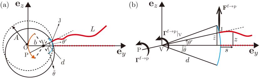
Figure 10: (a) Schematic of the model problem: a composite object of a sphere and a filament undergoes a rotational oscillation. The particle centre P and joint (filament base) J rotate periodically along circular arcs of radius $b$ and $d=A-b$, respectively. V denotes their common pivot point. (b) Zoom-in on the circular arc trajectory of the joint, showing the difference between the torque $\boldsymbol{\Gamma}^{\mathrm{f}\rightarrow\mathrm{p}}|_{V}$ with respect to the pivot V and $\boldsymbol{\Gamma}^{\mathrm{f}\rightarrow\mathrm{p}}$ to the particle centre P.

We find $\Gamma^{\mathrm{f}\rightarrow\mathrm{p}}_{N}(t)$ by solving a separate elastohydrodynamic problem of the composite object undergoing a prescribed rotational oscillation characterised by $\theta^{\prime}=\tilde{\theta}(t)\exp{\left(\mathrm{i}\sigma_{i}t\right)}$, where $\tilde{\theta}(t)=\Theta\exp{\left(\sigma_{r}t\right)}$ indicates the angular oscillation amplitude. We do not consider the object’s translation near the onset of instability since any translation is negligible due to the small-amplitude oscillation. To simplify the algebra in the next steps, we set $\hat{\theta}=\pi/2$ without loss of generality as shown in figure 10, where the rest configuration (dashed curves) corresponds to when the particle centre P coincides with the origin O and the undeformed filament is aligned in the $\mathbf{e}_{y}$ direction. The rotational oscillation is executed about a pivot V that lies away from the origin by a dimensional distance $b$ on the $y$-axis, where $\beta=b/L$; the dimensional distance between V and J is $d=A-b$, so similarly

$$\delta=d/L=\alpha-\beta.$$ (29)

The particle centre P (resp. filament base J) follows a trajectory of a circular arc that is centred at V and of radius $b$ (resp. $d$); both trajectories are symmetric about the $y$-axis. Note that $\beta$ is an unknown that is to be determined.

Near the onset of instability, the amplitude $\tilde{\theta}(t)$ varies much more slowly than the oscillation of $\theta^{\prime}$, viz. $\sigma_{r}\ll\sigma_{i}$. This allows us to assume that the amplitude $\tilde{\theta}=\Theta\exp{(\sigma_{r}t)}$ is quasi-steady, namely, $\theta^{\prime}$ at a particular time $t_{0}$ can be approximated by

$$\theta^{\prime}=\Theta\exp{\left(\sigma_{r}t_{0}\right)}\exp{\left(\mathrm{i}\sigma_{i}t\right)},$$ (30)

as an instantaneous configuration of a periodic signal with a prescribed amplitude $\Theta\exp{\left(\sigma_{r}t_{0}\right)}$ and frequency $\sigma_{i}$. This setup resembles the theoretical framework developed to address the so-called elastohydrodynamic problem II (Wiggins & Goldstein, 1998; Wiggins et al., 1998) of a filament with one of its ends undergoing straight, oscillatory translation. We adapt that framework for our configuration, whereas the filament end oscillates on a circular arc instead of on a straight path, as shown in figure 10b. Because the filament undergoes small-amplitude deformation, $|z_{y}|\ll 1$ and its tangent vector $\mathbf{r}_{s}\approxeq\mathbf{e}_{y}$. We also assume $T(s)\equiv 0$. The position $\mathbf{r}(t,s)$ of the filament centreline is $\mathbf{r}(s)=(\alpha+s)\mathbf{e}_{y}+z(t,s)\mathbf{e}_{z}$. The horizontal displacement of the filament base is of order $\mathcal{O}(\tilde{\theta}^{2})$ and can be neglected because $|\theta^{\prime}|\leq|\tilde{\theta}|\ll 1$. The base’s vertical oscillation is prescribed as

$$z(t)|_{s=0} =\delta\sin{\theta^{\prime}}\approxeq\delta\theta^{\prime}=\delta\tilde{\theta}\exp{(\mathrm{i}\sigma_{i}t)},$$ (31)

where $\delta\tilde{\theta}$ represents the oscillation amplitude. Following Wiggins & Goldstein (1998) and Wiggins et al. (1998), the deflection of the filament is expressed by

$$z(s)=\delta\tilde{\theta}\exp{(\mathrm{i}\sigma_{i}t)h(s,\mathcal{L})},$$ (32)

where

$$\mathcal{L}^{4}=\frac{\bar{\mu}\sigma_{i}}{-1-2\log{\epsilon_{\mathrm{sl}}}}$$ (33)

and $h$ is a sum of four solutions

$$h(s,\mathcal{L})=c_{1}\xi^{\mathrm{i}s}+c_{2}\xi^{-s}+c_{3}\xi^{-\mathrm{i}s}+c_{4}\xi^{s},$$ (34)

with

$$z_{0} =\exp{(-\mathrm{i}\pi/8)},$$ (35a)

$$\xi =\exp{(z_{0}\mathcal{L})}.$$ (35b)

The four coefficients $c_{i}$ need to be determined by the BCs at the filament ends. In contrast to Wiggins & Goldstein (1998) and Wiggins et al. (1998) treating $z(s)$ as a real variable, we consider a complex $z(s)$. This allows us to obtain the complex torque consistent with the complex nature of the torque balance, equation (28).

The BCs for $h(s)$ at the free end $s=1$ are $h_{ss}=h_{sss}=0$. At the clamped end $s=0$, $h=1$ as a Dirichlet BC corresponding to the prescribed displacement; the other BC is more subtle. Because the filament orientation is orthogonal to the circular arc (see figure 10b), we have

$$z_{s} =\sin{\theta^{\prime}}\approxeq\theta^{\prime}=\tilde{\theta}\exp{(\mathrm{i}\sigma_{i}t)}.$$ (36)

By substituting equation (32) into equation (36), we obtain the BC

$$h_{s}|_{s=0} =1/\delta,$$ (37)

where $\delta$ is defined in equation (29). Knowing all the BCs of $h(s)$, we compute the four coefficients

$$c_{1} =\frac{\left(1+\mathrm{i}\right)\left[\left((1-\mathrm{i})\xi^{1+\mathrm{i}}-\mathrm{i}\xi^{2}+1\right)\delta\log\xi-(1+\mathrm{i})\xi^{1+\mathrm{i}}-\mathrm{i}\xi^{2}-1\right]}{2\Lambda\delta\log\xi},$$ (38a)

$$c_{2} =\frac{\left(1+\mathrm{i}\right)\xi\left[\left(-\mathrm{i}\xi^{1+2\mathrm{i}}+(1-\mathrm{i})\xi^{\mathrm{i}}+\xi\right)\delta\log\xi-\xi^{1+2\mathrm{i}}+(-1+\mathrm{i})\xi^{\mathrm{i}}+\mathrm{i}\xi\right]}{2\Lambda\delta\log\xi},$$ (38b)

$$c_{3} =\frac{\left(1+\mathrm{i}\right)\xi^{\mathrm{i}}\left[\left(\xi^{2+\mathrm{i}}-\mathrm{i}\xi^{\mathrm{i}}+(1-\mathrm{i})\xi\right)\delta\log\xi+\xi^{2+\mathrm{i}}+\mathrm{i}\xi^{\mathrm{i}}+(1+\mathrm{i})\xi\right]}{2\Lambda\delta\log\xi},$$ (38c)

$$c_{4} =\frac{(1+\mathrm{i})\left(\xi^{2\mathrm{i}}+(1-\mathrm{i})\xi^{1+\mathrm{i}}-\mathrm{i}\right)\delta\log(\xi)+(1-\mathrm{i})\xi^{2\mathrm{i}}+2\xi^{1+\mathrm{i}}+1+\mathrm{i}}{2\Lambda\delta\log\xi},$$ (38d)

where $\Lambda=\xi^{2\mathrm{i}}+4\xi^{1+\mathrm{i}}+\xi^{2+2\mathrm{i}}+\xi^{2}+1$. Considering the small-amplitude deformation, the total force $\mathbf{F}$ exerted by the filament on the clamped end is along the vertical $\mathbf{e}_{z}$ direction. The torque $\boldsymbol{\Gamma}^{\mathrm{f}\rightarrow\mathrm{p}}|_{V}$ with respect to the pivot V and $\boldsymbol{\Gamma}^{\mathrm{f}\rightarrow\mathrm{p}}$ with respect to the particle centre P are along the $\mathbf{e}_{x}$ direction, so that the corresponding components of the force and torques are

$$F^{\mathrm{f}\rightarrow\mathrm{p}}_{z} =\tilde{\theta}\exp{\left(\mathrm{i}\sigma_{i}t\right)}\frac{\log^{2}{\xi}\left[(1+\mathrm{i})\Lambda_{1}\delta\log\xi-\mathrm{i}\Lambda_{2}\right]}{\Lambda},$$ (39a)

$$\Gamma^{\mathrm{f}\rightarrow\mathrm{p}}_{x}|_{V} =\tilde{\theta}\exp{\left(\mathrm{i}\sigma_{i}t\right)}\frac{\log\xi\left[(1+\mathrm{i})\delta^{2}\Lambda_{1}\log^{2}\xi-2\mathrm{i}\delta\Lambda_{2}\log\xi+(-1-\mathrm{i})\Lambda_{3}\right]}{\Lambda},$$ (39b)

$$\Gamma^{\mathrm{f}\rightarrow\mathrm{p}}_{x} =\Gamma^{\mathrm{f}\rightarrow\mathrm{p}}_{x}|_{V}+\left(\alpha-\delta\right)F^{\mathrm{f}\rightarrow\mathrm{p}}_{z}$$

$$=\tilde{\theta}\exp{\left(\mathrm{i}\sigma_{i}t\right)}\frac{\log\xi\left[(1+\mathrm{i})\alpha\delta\Lambda_{1}\log^{2}\xi-\mathrm{i}(\alpha+\delta)\Lambda_{2}\log\xi+(-1-\mathrm{i})\Lambda_{3}\right]}{\Lambda},$$ (39c)

where

$$\Lambda_{1} =-\xi^{2\mathrm{i}}-\mathrm{i}\xi^{2+2\mathrm{i}}+\xi^{2}+\mathrm{i},$$ (40a)

$$\Lambda_{2} =\left(-1+\xi^{2\mathrm{i}}\right)\left(\xi^{2}-1\right),$$ (40b)

$$\Lambda_{3} =\mathrm{i}\xi^{2\mathrm{i}}+\xi^{2+2\mathrm{i}}-\mathrm{i}\xi^{2}-1.$$ (40c)

Now, let us examine the denominator, $\Lambda$, of equation (39) whose five terms are in the form of $\xi^{q_{k}}$ ($k=1...5$), where $[q_{1},q_{2},q_{3},q_{4},q_{5}]=[2\mathrm{i},1+\mathrm{i},2+2\mathrm{i},2,0]$. Using equation (35), we express $\xi^{q_{k}}$ as

$$\xi^{q_{k}}=\left[\exp{(z_{0}\mathcal{L})}\right]^{q_{k}}=\zeta^{\mathcal{L}}_{k},$$ (41)

where $\zeta_{k}=\exp{(z_{0}q_{k})}$ are

$$\zeta_{1} =-0.59+2.09\mathrm{i},$$

$$\zeta_{2} =3.17+1.9\mathrm{i},$$

$$\zeta_{3} =6.4+12.05\mathrm{i},$$

$$\zeta_{4} =4.57-4.4\mathrm{i},$$

$$\zeta_{5} =1.$$ (42)

We observe that the third term $\zeta_{3}^{\mathcal{L}}$ is larger than the rest in magnitude when $\mathcal{L}\geq 1$, dominating the second largest term by one order when $\mathcal{L}\geq 3$. Let us assume $\mathcal{L}\geq 3$ a priori, so that we can then approximate $\Lambda$ by $\zeta_{3}^{\mathcal{L}}$ in equation (39). By further extracting the leading-order terms of $\Lambda_{1}/\Lambda$, $\Lambda_{2}/\Lambda$ and $\Lambda_{3}/\Lambda$, we attain a simplified, leading-order expression for the force and torque (denoted by $\;\tilde{\;}\;$)

$$\tilde{F}^{\mathrm{f}\rightarrow\mathrm{p}}_{z} =\tilde{\theta}\exp{\left(\mathrm{i}\sigma_{i}t\right)}\log^{2}{\xi}\left[(1-\mathrm{i})\delta\log\xi-\mathrm{i}\right],$$ (43a)

$$\tilde{\Gamma}^{\mathrm{f}\rightarrow\mathrm{p}}_{x}|_{\mathrm{V}} =\tilde{\theta}\exp{\left(\mathrm{i}\sigma_{i}t\right)}\log\xi\left[(1-\mathrm{i})\delta^{2}\log^{2}\xi-2\mathrm{i}\delta\log\xi-1-\mathrm{i}\right],$$ (43b)

$$\tilde{\Gamma}^{\mathrm{f}\rightarrow\mathrm{p}}_{x} =\tilde{\theta}\exp{\left(\mathrm{i}\sigma_{i}t\right)}\log\xi\left[(1-\mathrm{i})\alpha\delta\log^{2}\xi-\mathrm{i}(\alpha+\delta)\log\xi-1-\mathrm{i}\right].$$ (43c)

The theoretical force $F^{\mathrm{f}\rightarrow\mathrm{p}}_{z}$, torque $\Gamma^{\mathrm{f}\rightarrow\mathrm{p}}_{x}|_{\mathrm{V}}$ and their leading-order counterparts $\tilde{F}^{\mathrm{f}\rightarrow\mathrm{p}}_{z}$ and $\tilde{\Gamma}^{\mathrm{f}\rightarrow\mathrm{p}}_{x}|_{\mathrm{V}}$ are validated against the numerical results for six cases spanning a wide range of parameters relevant to our study (see table. 1), where case 1 is the reference case and the other five vary a single parameter compared to case 1. Because the numerical force and torque are real quantities, the real parts of $F^{\mathrm{f}\rightarrow\mathrm{p}}_{z}$ (dashed curve) given by equation (39a), and its leading-order approximation $\tilde{F}^{\mathrm{f}\rightarrow\mathrm{p}}_{z}$ (dot-dashed curve) by equation (43a), are compared with the numerical data (solid curve) in figure 11. A similar comparison between the torques $\Gamma^{\mathrm{f}\rightarrow\mathrm{p}}_{x}|_{\mathrm{V}}$ and $\tilde{\Gamma}^{\mathrm{f}\rightarrow\mathrm{p}}_{x}|_{\mathrm{V}}$ is shown in figure 12.

	$\tilde{\theta}$	$\delta$	$\sigma_{i}$	$\bar{\mu}$
Case 1 (reference)	$10^{-3}$	$0.3$	$0.2$	$10^{3}$
Case 2	$\mathbf{0.1}$	$0.3$	$0.2$	$10^{3}$
Case 3	$10^{-3}$	$\mathbf{0.8}$	$0.2$	$10^{3}$
Case 4	$10^{-3}$	$0.3$	$\mathbf{2}$	$10^{3}$
Case 5	$10^{-3}$	$0.3$	$0.2$	$\mathbf{10^{2}}$
Case 6	$10^{-3}$	$0.3$	$0.2$	$\mathbf{10^{4}}$

Table 1: Parameters for the six cases chosen to validate numerical results against the theoretical force $F^{\mathrm{f}\rightarrow\mathrm{p}}_{z}$, torque $\Gamma^{\mathrm{f}\rightarrow\mathrm{p}}_{x}|_{\mathrm{V}}$ and their leading-order counterparts. Bold entries indicate the difference with the reference, case $1$.

We observe that the force $F^{\mathrm{f}\rightarrow\mathrm{p}}_{z}$ and torque $\Gamma^{\mathrm{f}\rightarrow\mathrm{p}}_{x}|_{\mathrm{V}}$ and their leading-order values agree with the numerical results quantitatively in all the cases except for case $5$, where the leading-order results deviate a little from the full expression and numerical results. This disagreement results from the violation of the assumption $\mathcal{L}\geq 3$ used to derive the leading-order expression, where $\mathcal{L}\approx 1.25$ for case $5$. This also implies that the leading-order predictions become less accurate at small $\bar{\mu}$ values.

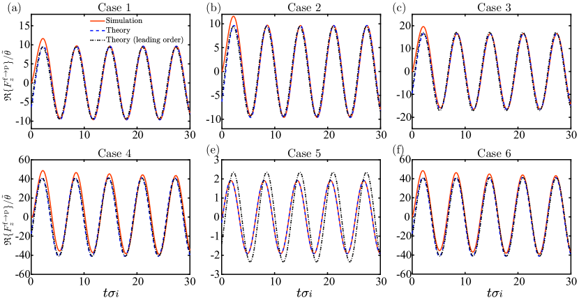
Figure 11: Comparison between the theoretical force $F^{\mathrm{f}\rightarrow\mathrm{p}}_{z}$ (dashed curves), its leading-order approximation $\tilde{F}^{\mathrm{f}\rightarrow\mathrm{p}}_{z}$ (dot-dashed curves) and the numerical results (solid curves).

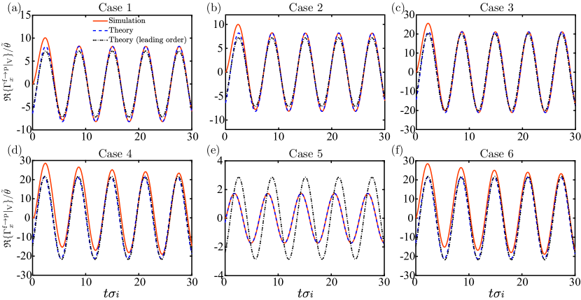
Figure 12: Comparison between the theoretical torque $\Gamma^{\mathrm{f}\rightarrow\mathrm{p}}_{x}|_{\mathrm{V}}$ (dashed curves), its leading-order approximation $\tilde{\Gamma}^{\mathrm{f}\rightarrow\mathrm{p}}_{x}|_{\mathrm{V}}$ (dot-dashed curves) and the numerical results (solid curves).

For the validation purpose, $\delta=\alpha-\beta$ can be prescribed. However, for the model, $\delta$ needs to be determined using the force-free condition on the particle. The particle follows a circular arc on the other side of the pivot V, the $z$-component of the hydrodynamic force on the particle approximated by the Stokes’s law is

$$F_{z}^{\mathrm{h}\rightarrow\mathrm{p}}=\frac{3\mathrm{i}}{4}\bar{\mu}\alpha\beta\sigma_{i}\tilde{\theta}\exp{\left(\mathrm{i}\sigma_{i}t\right)}.$$ (44)

Substituting equation (43a) and (44) into $\tilde{F}^{\mathrm{f}\rightarrow\mathrm{p}}_{z}+F_{z}^{\mathrm{f}\rightarrow\mathrm{p}}=0$, we obtain

$$\beta =\frac{4\log^{2}{\xi}\left[1+\alpha\left(\mathrm{i}+1\right)\log{\xi}\right]}{3\alpha\bar{\mu}\sigma_{i}+4\left(\mathrm{i}+1\right)\log^{3}{\xi}}.$$ (45)

Using the leading-order torque $\tilde{\Gamma}^{\mathrm{f}\rightarrow\mathrm{p}}_{x}$ equation (43c), as the left-hand side torque of equation (28) (note that the nodal line direction $\mathbf{N}=\mathbf{e}_{x}$ when the orientation $\mathbf{e}_{\mathrm{p}}$ is restricted to the $yz$-plane), we obtain the governing equation for the transformed growth rate $\hat{\sigma}=\bar{\mu}\sigma$,

$$\alpha^{3}\frac{\hat{\sigma}\left[\hat{\sigma}-\left(\bar{E}^{2}-1\right)\kappa\bar{\mu}\right]}{\hat{\sigma}+\kappa\bar{\mu}}+\log\xi\left[(\mathrm{i}-1)\alpha(\alpha-\beta)\log^{2}\xi+\mathrm{i}(2\alpha-\beta)\log\xi+1+\mathrm{i}\right]=0,$$ (46)

where

$$\beta =\frac{4\log^{2}{\xi}\left[1+\alpha\left(\mathrm{i}+1\right)\log{\xi}\right]}{3\alpha\hat{\sigma}_{i}+4\left(\mathrm{i}+1\right)\log^{3}{\xi}},$$ (47)

where $\log{\xi}$ can be written as

$$\log{\xi}=z_{0}\mathcal{L}=z_{0}\left(\frac{\hat{\sigma}_{i}}{-1-2\log{\epsilon_{\mathrm{sl}}}}\right)^{1/4}.$$ (48)

4.3 Complex growth rates and onset of instability

We solve equation (46) to obtain the transformed growth rate $\hat{\sigma}$, which facilitates a theoretical prediction of the onset of self-oscillatory instability. The growth rate $\hat{\sigma}=\hat{\sigma}_{r}+\mathrm{i}\hat{\sigma}_{i}$ depends on $\alpha$, $\epsilon_{\mathrm{sl}}$, $\kappa$, $\bar{\mu}$ and $E$, where we have fixed $\epsilon_{\mathrm{sl}}$ and $\kappa$. By writing $\hat{\sigma}_{i}=W^{4}$ and substituting it into equation (33), we obtain $\mathcal{L}=W/(-1-2\log{\epsilon_{\mathrm{sl}}})^{1/4}$. Here, $\mathcal{L}$ is a positive real number, so is $W$. By substituting equations (47) and (48) into equation (46), we derive a system of two-dimensional, nonlinear polynomial equations for $\hat{\sigma}_{r}$ and $W$ (see appendix C) and obtain its roots by employing the python driver phcpy (Verschelde, 2013; Otto et al., 2019) of a general-purpose solver PHCpack (Verschelde, 1997) for polynomial systems. Because $\hat{\sigma}=\bar{\mu}\sigma$, we obtain the real part $\sigma_{r}=\hat{\sigma}_{r}/\bar{\mu}$ and imaginary part $\sigma_{i}=W^{4}/\bar{\mu}$ of the complex growth rate $\sigma$.

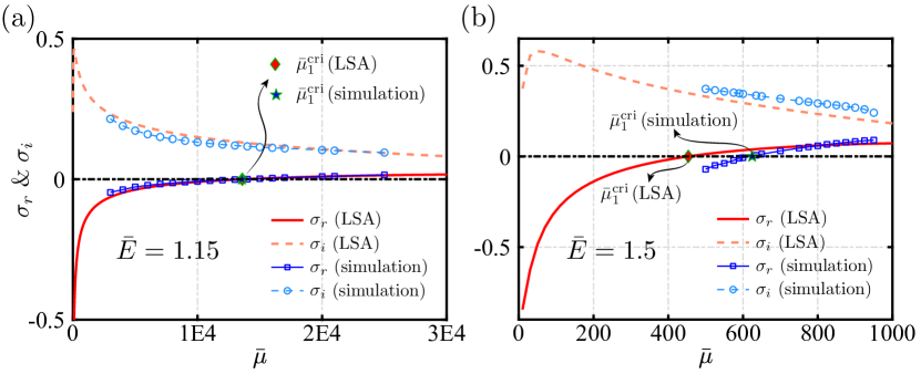
Figure 13: The real $\sigma_{r}$ and imaginary $\sigma_{i}$ part of the complex growth rate $\sigma=\sigma_{r}+\mathrm{i}\sigma_{i}$ versus $\bar{\mu}$ for two electric fields (a) $\bar{E}=1.15$ and (b) $\bar{E}=1.5$, where the size ratio $\alpha=0.3$. Theoretical (LSA) and numerical predictions are denoted by red curves and blue symbols, respectively. The intersection of $\sigma_{r}(\bar{\mu})$ with $\sigma=0$ gives the critical EEV value $\bar{\mu}_{1}^{\mathrm{cri}}$ (indicated by diamonds and pentagrams for theoretical and numerical results, respectively) corresponding to the onset of instability.

We show $\sigma_{r}$ and $\sigma_{i}$ as a function of $\bar{\mu}$ in figure 13 for two electric fields $\bar{E}=1.15$ (a) and $\bar{E}=1.5$ (b), where $\alpha=0.3$. In both cases, the imaginary part $\sigma_{i}\left(\bar{\mu}\right)>0$ implying that the perturbation always decays/grows in an oscillatory manner. In contrast, the real part $\sigma_{r}$ increases with $\bar{\mu}$ monotonically from negative to positive values, indicating the critical condition $\sigma_{r}\left(\bar{\mu}_{1}^{\mathrm{cri}}\right)=0$ of the self-oscillatory instability. When $\bar{\mu}$ is smaller/larger than $\bar{\mu}_{1}^{\mathrm{cri}}$, the perturbation exhibits oscillatory decaying and growth. The LSA prediction of $\left(\sigma_{r},\sigma_{i}\right)$ agrees quantitatively with the numerical counterpart for the $\bar{E}=1.15$ case, and qualitatively for the $\bar{E}=1.5$ case.

We adopt a bi-section method to determine $\bar{\mu}_{1}^{\mathrm{cri}}$ as a function of $\left(\bar{E},\alpha\right)$, as shown in figure 14. For all $\alpha$ values, $\bar{\mu}_{1}^{\mathrm{cri}}$ decreases monotonically with $\bar{E}$. The theoretical and numerical predictions agree well with each other, especially in the high $\bar{\mu}$ regime. The agreement degenerates with decreasing $\bar{\mu}$. We infer that $\mathcal{L}$ becomes smaller when $\bar{\mu}$ decreases, hence this disagreement is mostly attributed to violating the $\mathcal{L}\geq 3$ assumption of the leading-order force/torque model for the LSA.

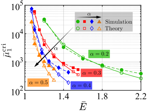
Figure 14: The LSA (hollow symbols) and numerical (filled symbols) predictions of the critical EEV number $\bar{\mu}_{1}^{\mathrm{cri}}$ (versus $\bar{E}$) at which instability occurs through a Hopf bifurcation, for size ratios $\alpha=0.2$ (circles), $0.3$ (squares), $0.4$ (diamonds) and $0.5$ (triangles).

5 A minimal model to reproduce the EEH instability and self-oscillation

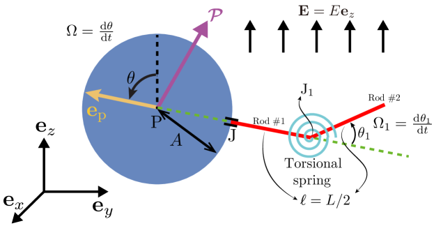
Figure 15: Schematic of a minimal model to reproduce the EEH instability and self-oscillation: the elastic filament is represented by two rigid rods of the same length $\ell=L/2$ linked flexibly at $\mathrm{J}_{1}$ by a torsional spring of elastic modulus $K$. Rod $\#1$ is rigidly anchored at J. A steady, uniform electrical field $\mathbf{E}=E\mathbf{e}_{z}$ is applied.

To better unravel the physics underlying the EEH instability, we seek a minimal model reproducing this instability and the corresponding self-oscillation. By analogy to the multi-linker models (De Canio et al., 2017; Ling et al., 2018), we replace the elastic filament by two rigid cylindrical rods numbered $\#1$ and $\#2$ of equal length $\ell=L/2$ and equal radius $a$ of their cross sections, which are linked at $\mathrm{J}_{1}$ by a torsional spring with an elastic module of $K$ (see figure. 15). Rod $\#1$ is clamped at the sphere surface J, namely it always passes through the particle centre P, hence the displacement vectors $\overrightarrow{\mathrm{PJ}}$ and $\overrightarrow{\mathrm{P}\mathrm{J}_{1}}$ are opposite to the particle orientation $\mathbf{e}_{\mathrm{p}}$. Rod $\#2$ is oriented with respect to $\overrightarrow{\mathrm{P}\mathrm{J}_{1}}$ by an angle $\theta_{1}$, which is zero when the composite system is at rest.

Similar to the original setup, we assume that the motion of particle and the rods are restricted to the $yz$-plane. Further, no hydrodynamic interactions between the particle and rods, or between the rods are considered. The system consists of six unknowns: the translational velocity components $U_{y}(t)$ and $U_{z}(t)$ of the particle, the rotational velocity component $\frac{\mathrm{d}\theta(t)}{\mathrm{d}t}=\Omega(t)$ of the particle and $\frac{\mathrm{d}\theta_{1}(t)}{\mathrm{d}t}=\Omega_{1}(t)$ of rod $\#2$ with respect to rod $\#1$, and the polarisation vector components $\mathcal{P}_{Q}(t)$ and $\mathcal{P}_{3}(t)$. It is worth noting that compared to the classical QR particle, this minimal configuration only incorporates one extra degree of freedom, $\theta_{1}$, which indicates the deformation magnitude of the torsional spring.

We first derive the hydrodynamic force exerted on rod $\#1$ as

$$\mathbf{F}^{\mathrm{hydro}}_{1}= \frac{2\pi\mu\ell}{c}\left[2\theta_{t}(2A+\ell)\cos\theta+U_{y}\cos 2\theta+3U_{y}+U_{z}\sin 2\theta\right]\mathbf{e}_{y}$$

$$+ \frac{2\pi\mu\ell}{c}\left[2\theta_{t}(2A+\ell)\sin\theta+U_{y}\sin 2\theta-U_{z}\cos{2\theta}+3U_{z}\right]\mathbf{e}_{z},$$ (49)

and the torque about the particle centre P

$$\boldsymbol{\Gamma}^{\mathrm{hydro}}_{1}|_{\mathrm{P}}=\frac{4\pi\mu\ell}{3c}\left[2\theta_{t}\left(3A^{2}+3A\ell+\ell^{2}\right)+3U_{y}(2A+\ell)\cos\theta+3U_{z}(2A+\ell)\sin\theta\right]\mathbf{e}_{x}.$$ (50)

Likewise, the hydrodynamic force exerted on rod $\#2$ is

$$\mathbf{F}^{\mathrm{hydro}}_{2}=\frac{2\pi\mu\ell}{c}\left[\theta_{t}\left(A+\ell\right)\cos(\theta+2\theta_{1})+3\theta_{t}(A+\ell)\cos\theta+2\ell(\theta_{t}+\theta_{1,t})\cos(\theta+\theta_{1})+U_{y}\cos 2(\theta+\theta_{1})+3U_{y}+U_{z}\sin 2(\theta+\theta_{1})\right]\mathbf{e}_{y}\\ +\frac{2\pi\mu\ell}{c}\left[\theta_{t}\left(A+\ell\right)\sin(\theta+2\theta_{1})+3\theta_{t}(A+\ell)\sin\theta+2\ell\left(\theta_{t}+\theta_{1,t}\right)\sin(\theta+\theta_{1})+U_{y}\sin 2(\theta+\theta_{1})-U_{z}\cos 2(\theta+\theta_{1})+3U_{z}\right]\mathbf{e}_{z}$$ (51)

and the hydrodynamic torque on rod $\#2$ about $\mathrm{J}_{1}$ is

$$\boldsymbol{\Gamma}^{\mathrm{hydro}}_{2}|_{\mathrm{J}_{1}}=\frac{4\pi\mu\ell^{2}}{3c}\left[3\theta_{t}(A+\ell)\cos\theta_{1}+2\ell\left(\theta_{t}+\theta_{1,t}\right)+3U_{y}\cos(\theta+\theta_{1})+3U_{z}\sin(\theta+\theta_{1})\right].$$ (52)

The torque-free condition on rod $\#2$ reads

$$\mathbf{M}_{2}+\boldsymbol{\Gamma}^{\mathrm{hydro}}_{2}|_{\mathrm{J}_{1}}=\mathbf{0},$$ (53)

where $\mathbf{M}_{2}=-K\theta_{1}\mathbf{e}_{x}$ is the elastic moment exerted on rod $\#2$ by the torsional spring. The torque balance on the whole composite system about the particle centre P is

$$\boldsymbol{\Gamma}^{\mathrm{hydro}}_{1}|_{\mathrm{P}}+\underbrace{\left(\boldsymbol{\Gamma}^{\mathrm{hydro}}_{2}|_{\mathrm{J}_{1}}+\overrightarrow{\mathrm{P}\mathrm{J}_{1}}\times\mathbf{F}^{\mathrm{hydro}}_{2}\right)}_{\text{hydrodynamic torque on rod }\#2\text{ about P}}-\gamma_{\mathrm{drag}}\theta_{t}\mathbf{e}_{x}+\underbrace{\left(E_{3}\mathcal{P}_{Q}-E_{Q}\mathcal{P}_{3}\right)\mathbf{e}_{x}}_{\text{electric torque on the particle}}=\mathbf{0}.$$ (54)

We also need to impose the force-free condition on the whole composite object

$$\mathbf{F}^{\mathrm{hydro}}_{1}+\mathbf{F}^{\mathrm{hydro}}_{2}-\beta_{\mathrm{drag}}\left(U_{y}\mathbf{e}_{y}+U_{z}\mathbf{e}_{z}\right)=\mathbf{0}.$$ (55)

To close the system, we solve the governing equations (8b) and (8c) for $\mathcal{P}_{Q}$ and $\mathcal{P}_{3}$, where the second term $-\frac{\partial\psi}{\partial t}\mathcal{P}_{N}$ in equation (8b) disappears. We note that equations (53) and (54) indeed reflect the subtle interplay between the elastic, electric and hydrodynamic torques, which lead to the EEH instability-induced self-oscillation.

5.1 Nondimensionalization of the minimal model

We use the same characteristic scales as the original particle-filament configuration (see § 2) to nondimensionalise equations (53), (54) and (55), except that we substitute $D$ by $KL$, resulting in a slightly modified EEV parameter

$$\breve{\mu}=\frac{8\pi\mu L^{3}}{K\tau_{\mathrm{s}}},$$ (56)

to be distinguished from $\bar{\mu}$ defined by equation (11) for the original setup. The dimensionless governing equations for $\bar{U}_{y}(\bar{t})$, $\bar{U}_{z}(\bar{t})$, $\theta(\bar{t})$ and $\theta_{1}(\bar{t})$ are

$$\left(7\alpha+5/2\right)\bar{\Omega}\cos\theta+\bar{\Omega}\left(\alpha+1/2\right)\cos\left(\theta+2\theta_{1}\right)+\left(\bar{\Omega}+\bar{\Omega}_{1}\right)\cos\left(\theta+\theta_{1}\right)+\bar{U}_{y}\left[\cos 2\theta+\cos 2\left(\theta+\theta_{1}\right)-6\alpha c+6\right]+\bar{U}_{z}\left[\sin 2\theta+\sin 2\left(\theta+\theta_{1}\right)\right]=0,$$ (57a)

$$\left(7\alpha+5/2\right)\bar{\Omega}\sin{\theta}+\bar{\Omega}\left(\alpha+1/2\right)\sin\left(\theta+2\theta_{1}\right)+\left(\bar{\Omega}+\bar{\Omega}_{1}\right)\sin\left(\theta+\theta_{1}\right)+\bar{U}_{z}\left[-\cos 2\theta-\cos 2\left(\theta+\theta_{1}\right)-6\alpha c+6\right]+\bar{U}_{y}\left[\sin{2\theta}+\sin 2\left(\theta+\theta_{1}\right)\right]=0,$$ (57b)

$$\frac{\breve{\mu}}{24}\left[3\bar{\Omega}\left(\alpha+1/2\right)\cos\theta_{1}+\bar{\Omega}+\bar{\Omega}_{1}+3\bar{U}_{y}\cos\left(\theta+\theta_{1}\right)+3\bar{U}_{z}\sin\left(\theta+\theta_{1}\right)\right]-c\theta_{1}=0,$$ (57c)

$$\frac{\breve{\mu}}{24}\left\{\left(21\alpha^{2}+15\alpha+13/4\right)\bar{\Omega}+3\left(\alpha+1/2\right)\left(\bar{\Omega}+\bar{\Omega}_{1}\right)\cos\theta_{1}\\ +3\left(7\alpha+5/2\right)\left(\bar{U}_{y}\cos{\theta}+\bar{U}_{z}\sin{\theta}\right)\\ +3\left(\alpha+1/2\right)\cos 2\theta_{1}\left[\left(\alpha+1/2\right)\bar{\Omega}+\bar{U}_{y}\cos\theta+\bar{U}_{z}\sin\theta\right]+3\left(\alpha+1/2\right)\sin 2\theta_{1}\left(\bar{U}_{z}\cos\theta-\bar{U}_{y}\sin\theta\right)\right\}\\ +c\theta_{1}-c\bar{\eta}\bar{\Omega}+c\bar{E}\left(\bar{\mathcal{P}}_{Q}\cos\theta-\bar{\mathcal{P}}_{3}\sin\theta\right)=0,$$ (57d)

where $c=1+2\log\epsilon_{\mathrm{sl}}$ and $\bar{\eta}=\alpha^{3}\breve{\mu}$ as given by equations (16) and (10), respectively.

The dimensionless equations for $\bar{\mathcal{P}}_{Q}$ and $\bar{\mathcal{P}}_{3}$ are

$$\frac{\partial\bar{\mathcal{P}}_{Q}}{\partial\bar{t}} =-\kappa\left(\bar{\mathcal{P}}_{Q}+\kappa\bar{\eta}\bar{E}\sin\theta\right),$$ (58a)

$$\frac{\partial\bar{\mathcal{P}}_{3}}{\partial\bar{t}} =-\kappa\left(\bar{\mathcal{P}}_{3}+\kappa\bar{\eta}\bar{E}\cos\theta\right),$$ (58b)

with their initial values at $\bar{t}=0$

$$\bar{\mathcal{P}}_{Q}\left(\bar{t}=0\right) =\frac{\bar{\eta}\kappa^{2}\bar{E}\sin\theta}{\kappa-\left(R-1\right)/\left(S-1\right)},$$ (59a)

$$\bar{\mathcal{P}}_{3}\left(\bar{t}=0\right) =\frac{\bar{\eta}\kappa^{2}\bar{E}\cos\theta}{\kappa-\left(R-1\right)/\left(S-1\right)}.$$ (59b)

5.2 Numerical and theoretical (LSA) results of the minimal model

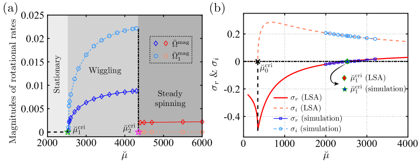
Figure 16: (a) Numerical results of the rotational velocity magnitudes of the minimal model versus $\breve{\mu}$ by solving equations (57) and (58), where $\left(\bar{E},\alpha\right)=\left(1.5,0.3\right)$; diamonds and circles denote those of the particle and rod $\#2$, respectively. $\breve{\mu}_{1}^{\mathrm{cri}}$ and $\breve{\mu}_{2}^{\mathrm{cri}}$ separate the three $\breve{\mu}$-dependent regimes: stationary, wiggling (blue) and steady spinning (red). (b) LSA (red) and numerical (blue) results of the real $\sigma_{r}$ and imaginary $\sigma_{i}$ parts of the complex growth rate $\sigma$ versus $\breve{\mu}$, where $\left(\bar{E},\alpha\right)=\left(1.5,0.3\right)$. $\breve{\mu}_{0}^{\mathrm{cri}}$ distinguishes whether the perturbations decay monotonically when $\breve{\mu}<\breve{\mu}_{0}^{\mathrm{cri}}$ or in an oscillatory manner when $\breve{\mu}_{0}^{\mathrm{cri}}<\breve{\mu}<\breve{\mu}_{1}^{\mathrm{cri}}$.

We solve equations (57) and (58) numerically using the MATLAB solver ‘ode15s’ for ordinary differential equations. Fixing the electric field $\bar{E}=1.5$ and size ratio $\alpha=0.3$, we show in figure 16a the $\breve{\mu}$-dependent magnitudes $\bar{\Omega}^{\mathrm{mag}}$ and $\bar{\Omega}^{\mathrm{mag}}_{1}$ of the rotational velocities of the particle and rod $\#2$, respectively, when the minimal composite object reaches its equilibrium configuration. This simple model reproduces the three characteristic behaviours of the original particle-filament system: stationary ($\breve{\mu}<\breve{\mu}_{1}^{\mathrm{cri}}\approx 2513$), wiggling ($\breve{\mu}_{1}^{\mathrm{cri}}<\breve{\mu}<\breve{\mu}_{2}^{\mathrm{cri}}\approx 4300$) and steady spinning ($\breve{\mu}>\breve{\mu}_{2}^{\mathrm{cri}}$). In the spinning state, $\bar{\Omega}^{\mathrm{mag}}_{1}=|\mathrm{d}\theta_{1}/\mathrm{d}\bar{t}|=0$ reflects a time-independent angle $\theta_{1}$ between the two rods, which adopt a steady “deformed” configuration representing a minimal model of the deformed filament.

Conducting an LSA for this minimal model, we find the closed-form expression of the complex growth rate $\sigma=\sigma_{r}+\mathrm{i}\sigma_{i}$ (see appendix D for details). The theoretical values of $\sigma_{r,i}$ versus $\breve{\mu}$ in case of $\left(\bar{E},\alpha\right)=\left(1.5,0.3\right)$ are depicted in figure 16b, as well as their numerical counterparts in the near $\breve{\mu}_{1}^{\mathrm{cri}}$ regime. The theoretical and numerical values of both $\sigma_{r}$ and $\sigma_{i}$ almost lie on top of each other, consequently, their predictions of $\breve{\mu}_{1}^{\mathrm{cri}}$ (when $\sigma_{r}=0$) agree. This superior agreement to the particle-filament system (figure 13) is expected, because the minimal model does not require an approximate model (see §4.2) for the elastic torque as the original case.

The LSA also indicates the emergence of another subtle critical EEV number $\breve{\mu}_{0}^{\mathrm{cri}}\approx 345$ (black cross in figure 16b): when $\breve{\mu}<\breve{\mu}_{0}^{\mathrm{cri}}$, the real part $\sigma_{r}$ of the growth rate is negative, accompanying a zero imaginary part, thus the perturbations diminish to zero monotonically; when $\breve{\mu}_{0}^{\mathrm{cri}}<\breve{\mu}<\breve{\mu}_{1}^{\mathrm{cri}}$, $\sigma_{r}<0$ but $\sigma_{i}>0$, the perturbations also die out but in a an oscillatory fashion. The former case corresponds to the non-negative quantity $\Sigma$ inside the square-root operator in equation (85) that naturally yields real solutions for $\sigma$ only. A similar structure of the solutions of $\sigma$ was reported in De Canio et al. (2017). Since the current work mainly addresses the EEH instability-induced self-oscillation, we do not pursue a detailed investigation in this stable, stationary regime.

6 Conclusions and discussions

Standard biomimetic practises commonly rely on an oscillating magnetic or electric field to produce the oscillatory motion of slender artificial structures. In contrast, we propose a strategy to achieve self-oscillation of artificial structures based on a time-independent, uniform electric field. By formulating and numerically solving an elasto-electro-hydrodynamic problem, this concept is illustrated by oscillating a composite object consisting of a weakly conducting dielectric spherical particle and an elastic filament immersed in a dielectric solvent.

Our strategy is grounded in the QR electrohydrodynamic instability phenomenon indicating that a weakly conducting dielectric particle suspended in a dielectric liquid of higher conductivity can undergo spontaneous rotation under a sufficiently strong DC electric field. For an individual spherical particle, this instability emerges through a supercritical pitchfork bifurcation resulting in steady rotation (Jones, 1984). By incorporating an elastic filament, we transform the pitchfork bifurcation into a Hopf bifurcation through which a self-oscillatory instability occurs (Zhu & Stone, 2019). This transformation is attributed to the elasto-viscous response of the filament providing an elastic torque to balance the electric and hydrodynamic torques. The elastic torque is in phase with the rotational velocity of the particle at certain time periods (see figure 9b). This in-phase behaviour results in negative damping (or positive feedback), hence leading to the onset of linear instability (Jenkins, 2013). We comment that such a transition from pitchfork to Hopf bifurcation was also identified by Tsebers (1980a) who observed oscillatory QR of ellipsoidal particles attributed to their anisotropic electric properties. It is also worth mentioning that the QR instability was utilised to study suspensions of artificial swimmers made of QR particles that achieved locomotion by rolling near a rigid solid boundary (Bricard et al., 2013). In addition, the recent work of Das & Lauga (2019) shows theoretically and numerically that a dielectric particle with particular geometrical asymmetry (e.g. a helix) under a DC electric field is able to convert QR into spontaneous translation in an unbounded domain.

We next recall the original experiments conducted by Quincke (1896), where the particle was hung by a silk thread and hence the particle rotated in the direction along the orientation of the thread. Quincke also noted an oscillatory behaviour as translated by Jones (1984)

“Quincke, with his spheres tethered to silk threads, had been forced to contend with periodic rotation, first in one direction and then in the other as the silk thread wound and unwound”.

We think that the “wound and unwound” motion manifested the self-oscillatory phenomenon, which is attributed to the torsional deformation of the silk thread. We speculate that Quincke probably regarded this observation as an experimental nuisance, thus did not pay attention to it nor did other researchers, except for one little-known preprint (Zaks & Shliomis, 2014) that recognised and modelled this torsional oscillation by considering a QR particle hung by a thread with torsional elasticity.

In this paper, we consider only the bending stiffness of the grafted filament and the whole composite object is freely suspended in the solvent. By applying an electric field stronger than the critical value corresponding to the onset of original QR instability, the composite object exhibits three distinct behaviours depending on the EEV number $\bar{\mu}$ (inversely proportional to the bending stiffness). When $\bar{\mu}\leq\bar{\mu}_{1}^{\mathrm{cri}}$, the object remains stationary, corresponding to a fixed-point solution; when $\bar{\mu}\geq\bar{\mu}_{2}^{\mathrm{cri}}$, the particle spins steadily towing a deformed filament, corresponding to an asymmetric fixed-point solution; when $\bar{\mu}\in\left(\bar{\mu}_{1}^{\mathrm{cri}},\bar{\mu}_{2}^{\mathrm{cri}}\right)$, the particle oscillates and the filament wiggles, leading the object to an undulatory locomotion. More specifically, instability occurs at $\bar{\mu}_{1}^{\mathrm{cri}}$ through a supercritical Hopf bifurcation, where the self-oscillatory motion represents a limit-cycle solution; at $\bar{\mu}_{2}^{\mathrm{cri}}$, a secondary bifurcation appears, and the oscillatory, limit-cycle solution jumps to the steadily spinning, fixed-point solution. By fixing the EEV number $\bar{\mu}$, bifurcation diagrams considering the electric field strength $\bar{E}$ as the control parameter revealed the same three scenarios (see figure 8).

We have also examined the propulsive performance of the micro object in the self-oscillating regime $\bar{\mu}\in(\bar{\mu}_{1}^{\mathrm{cri}},\bar{\mu}_{2}^{\mathrm{cri}})$. The trajectory of the object resembles a wave propagating along a straight path. The translational velocity of the object along this path varies in $\bar{\mu}$ non-monotonically (see figure 7c).

Motivated by the exponential temporal growth of the rotational velocity, we performed a LSA to predict theoretically the onset of the self-oscillatory instability. We have developed an elastohydrodynamic model to account for the elastic force and torque exerted by the filament on the particle, which closely matched the numerical counterparts. Incorporating this model into a standard LSA for the original QR particle, we derived the dispersion relationship of the new EEH problem. We thus calculated the complex growth rate $\sigma=\sigma_{r}+\mathrm{i}\sigma_{i}$ and identified the critical EEV number $\bar{\mu}_{1}^{\mathrm{cri}}$. Theoretical predictions of $\sigma$ (figure 13) and $\bar{\mu}_{1}^{\mathrm{cri}}$ (figure 14) agree well the numerical results, especially in the large $\bar{\mu}$ regime. However, the agreement becomes less satisfactory when $\bar{\mu}$ decreases because of the violation of an assumption used in the elastohydrodynamic model.

To unravel the EEH instability mechanism, we studied a minimal model system characterised by two rigid rods linked by a torsional spring to mimic the original filament. This substitution reduces the elastic element’s number of degrees of freedom to one. Numerical and LSA results demonstrated that the minimal model could exhibit the three elasticity-dependent behaviours: stationary, wiggling and steady spinning.

Following the comments of an anonymous referee, we hereby emphasise the difference between our work and other seemingly similar studies (Manghi et al., 2006; Qian et al., 2008; Coq et al., 2008), where a flexible slender structure (filament or rod) rotated in a viscous fluid and produced thrust because one of its ends was clamped to a constantly rotating base or actuated by a constant torque. This rotation results from forced oscillation characterised by a close correlation between the frequency of the power source and that of the resulting periodic motion. This forced-oscillatory periodic motion distinguishes itself from the self-oscillatory motion we observe, where the time-independent electric field as the power source lacks a frequency corresponding to that of the periodic motion.

The current work constrained the kinematics and electric polarisation vector of the particle to a plane in order to show a clean physical picture of the new EEH instability we identified. By removing these constraints, we anticipate the appearance of more complex and diverse three-dimensional behaviours featured by bi/multi-stability, hysteresis and even chaos (ellipsoidal particles were observed to exhibit chaotic QR (Tsebers, 1991)). We will report the results of the ongoing work in a future paper.

It is also worth mentioning the assumption of neglecting electrohydrodynamic effect of the filament. The electric torque exerted on a slender QR structure scales with $a^{2}L$ (Das & Lauga, 2019), and that on a sphere scales with $A^{3}$ (see equation (69)). By assuming that the filament and particle have similar dielectric properties and realising $\alpha=A/L=O(1)$, the ratio of the former to the latter torque is of the order of $\epsilon_{\mathrm{sl}}^{2}$. This comparison thus justifies the assumption, which also implies that no special attention needs to be paid in this context for the experimental realisation.

In conclusion, incorporating an elastic element to manipulate the electrohydrodynamic instability, we report an elasto-electro-hydrodynamic instability and use it for engineering self-oscillation of artificial structures. We anticipate that this idea of harnessing elastic media to control and diversify the bifurcation and the corresponding instability behaviour can be generalised to other stability phenomena and systems. As a result, different emerging instability behaviours can be utilised for diverse functionalities. This concept might inspire new approaches to design soft, reconfigurable machines that can morph and adapt to the environment.

Declaration of Interests. The authors report no conflict of interest.

Appendix A Numerical methods for the EEH problem

In this section, we describe the numerical methods to solve the EEH problem. For notation brevity, we remove all the bars over the unknown dimensionless variables henceforth. Following Tornberg & Shelley (2004), we use a finite difference scheme to discretise the filament centreline by a uniform grid of $N$ points. A typical value of $N=201$ is used in the simulations. Therefore, we have $N$ unknowns for the tension $T(s)$ and $3N$ for the coordinates $\mathbf{r}(s)=x\mathbf{e}_{x}+y\mathbf{e}_{y}+z\mathbf{e}_{z}$. The implementation considers a general three-dimensional motion of the filament, hence we also solve for $x(s)$ even though the motion is restricted to the $yz$-plane.

In contrast, for the restricted motion of the particle, we express its translational velocity $\mathbf{U}$ and rotational velocity $\boldsymbol{\Omega}$ as

$$\mathbf{U} =U_{y}\mathbf{e}_{y}+U_{z}\mathbf{e}_{z},$$ (60a)

$$\boldsymbol{\Omega} =\Omega\mathbf{e}_{x}=\theta_{t}\mathbf{e}_{x},$$ (60b)

which yields three unknowns $U_{y}$, $U_{z}$ and $\Omega=\theta_{t}$ for the particle. Another two unknowns are $\mathcal{P}_{Q}$ and $\mathcal{P}_{3}$ governed by equations (12b) and (12c), respectively.

At the $(k+1)$-th time step, $T^{k+1}(s)$ is solved based on $\mathbf{r}^{k}(s)$ at the $k$-th time step. We then solve $[\mathbf{r}^{k+1}(s),U^{k+1}_{y},U^{k+1}_{z},\Omega^{k+1},\mathcal{P}^{k+1}_{Q},\mathcal{P}^{k+1}_{3}]$ in a coupled way, which consists of $3N+5$ unknowns. We adopt this coupled strategy to accurately preserve the clamped BC of the filament base J ($s=0$): first, the filament base is on the particle surface; second, the tangent vector $\mathbf{r}_{s}|_{s=0}$ at the base always passes through the particle centre P. This clamped BC of the filament is different from other configurations (Guglielmini et al., 2012; De Canio et al., 2017) where the base is stationary. In our case, the filament base is right on the particle surface, and is able to translate with and rotate about the particle centre.

We use the backward Euler formulation to approximate the particle centre $\mathbf{x}_{\mathrm{p}}^{k+1}$,

$$\mathbf{x}_{\mathrm{p}}^{k+1}=\mathbf{x}_{\mathrm{p}}^{k}+\Delta t\mathbf{U}^{k+1},$$ (61)

where $\Delta t$ is the time step. The Dirichlet BC for $\mathbf{r}|_{s=0}$, namely equation (21a) becomes

$$\mathbf{r}^{k+1} =\mathbf{x}_{\mathrm{p}}^{k}+\Delta t\mathbf{U}^{k+1}+\alpha\mathbf{r}_{s}^{k+1}.$$ (62)

Likewise, we write $\theta^{k+1}=\theta^{k}+\Delta t\Omega^{k+1}$. By assuming $\Delta t\Omega\ll 1$, we obtain

$$\cos{\theta^{k+1}} \approx\cos{\theta^{k}}-\left(\Delta t\sin{\theta^{k}}\right)\Omega^{k+1},$$ (63a)

$$\sin{\theta^{k+1}} \approx\sin{\theta^{k}}+\left(\Delta t\cos{\theta^{k}}\right)\Omega^{k+1}.$$ (63b)

The tangent vector $\mathbf{r}^{k+1}_{s}$ at the filament base is opposite to the particle orientation $\mathbf{e}_{\mathrm{p}}$, namely $\mathbf{r}^{k+1}_{s}=\sin{\theta^{k+1}}\mathbf{e}_{y}-\cos{\theta^{k+1}}\mathbf{e}_{z}$. Using equation (63), the discretised form of this BC is,

$$\mathbf{r}_{s}^{k+1}-\left(\Delta t\cos{\theta^{k}}\right)\Omega^{k+1}\mathbf{e}_{y}-\left(\Delta t\sin{\theta^{k}}\right)\Omega^{k+1}\mathbf{e}_{z} =\sin{\theta^{k}}\mathbf{e}_{y}-\cos{\theta^{k}}\mathbf{e}_{z}.$$ (64)

Combining equation (14a) and (23a), the discretised form for the force-free condition reads

$$-y^{k+1}_{sss}|_{s=0}+\left(T^{k+1}y^{k+1}_{s}\right)|_{s=0}-3\alpha\bar{\mu}U_{y}^{k+1}/4 =0,$$ (65a)

$$-z^{k+1}_{sss}|_{s=0}+\left(T^{k+1}z^{k+1}_{s}\right)|_{s=0}-3\alpha\bar{\mu}U_{z}^{k+1}/4 =0.$$ (65b)

Combining equation (14b) and (23b) similarly, the torque-free condition reads

$$\bar{\eta}\Omega=\bar{E}\cos{\theta}\mathcal{P}_{Q}-\bar{E}\sin{\theta}\mathcal{P}_{3}+\left[\left(\sin\theta\mathbf{e}_{y}-\cos\theta\mathbf{e}_{z}\right)\times\left(\mathbf{r}_{ss}-\alpha\mathbf{r}_{sss}\right)\right]|_{s=0}.$$ (66)

We approximate $\theta^{k+1}$ by $\check{\theta}=2\theta^{k}-\theta^{k-1}$ and substitute it into equation (66), deriving the discretised torque-free condition

$$\bar{\eta}\Omega^{k+1}=\bar{E}\cos{\check{\theta}}\mathcal{P}^{k+1}_{Q}-\bar{E}\sin{\check{\theta}}\mathcal{P}^{k+1}_{3}+\left[\left(\sin\check{\theta}\mathbf{e}_{y}-\cos\check{\theta}\mathbf{e}_{z}\right)\times\left(\mathbf{r}^{k+1}_{ss}-\alpha\mathbf{r}^{k+1}_{sss}\right)\right]|_{s=0}.$$ (67)

Using the backward Euler scheme for $\mathcal{P}_{Q}$ and $\mathcal{P}_{3}$, and combining equations (63), we find the discretised governing equations for $\mathcal{P}_{Q}$ and $\mathcal{P}_{3}$,

$$\left(\kappa+1/\Delta t\right)\mathcal{P}_{Q}^{k+1}+\kappa^{2}\bar{\eta}\bar{E}\Delta t\cos\theta^{k}\Omega^{k+1} =\mathcal{P}_{Q}^{k}/\Delta t-\kappa^{2}\bar{\eta}\bar{E}\sin\theta^{k},$$ (68a)

$$\left(\kappa+1/\Delta t\right)\mathcal{P}_{3}^{k+1}-\kappa^{2}\bar{\eta}\bar{E}\Delta t\sin\theta^{k}\Omega^{k+1} =\mathcal{P}_{3}^{k}/\Delta t-\kappa^{2}\bar{\eta}\bar{E}\cos\theta^{k}.$$ (68b)

Integrating equations (18), (65), (66) and (68), with the four BCs equations (20a), (62) and (64) for $\mathbf{r}^{k+1}$ generates a linear system of size $3N+5$. Its solution corresponds to $[\mathbf{r}^{k+1}(s),U^{k+1}_{y},U^{k+1}_{z},\Omega^{k+1},\mathcal{P}^{k+1}_{Q},\mathcal{P}^{k+1}_{3}]$.

Appendix B Quincke rotation of a dielectric sphere jointed with a rigid rod

Following Jones (1984), we derive the critical electric field required to trigger the electrohydrodynamic instability of a dielectric spherical particle grafted by a rigid rod. Let us first briefly reproduce the derivation of Jones (1984) for an individual particle and then extend it to our composite particle-rod configuration.

The electric torque exerted on a spherical particle of radius $A$ about its centre P is

$$\boldsymbol{\Gamma}^{\mathrm{elec}} =\frac{6\pi\epsilon_{\mathrm{s}}A^{3}E^{2}\left(1-R/S\right)\tau_{\mathrm{MW}}\Omega}{\left(1+\frac{2}{S}\right)\left(1+\frac{R}{2}\right)\left[1+\Omega^{2}{(\tau_{\mathrm{MW}})}^{2}\right]}\mathbf{e}_{x}.$$ (69)

When the particle rotates about its centre at velocity $\Omega\mathbf{e}_{x}$, the hydrodynamic torque exerted on it is

$$\boldsymbol{\Gamma}_{\mathrm{par}}^{\mathrm{hydro}} =-8\pi\mu A^{3}\Omega\mathbf{e}_{x}.$$ (70)

By using the torque-free condition $\boldsymbol{\Gamma}^{\mathrm{elec}}+\boldsymbol{\Gamma}^{\mathrm{hydro}}_{\mathrm{par}}=\mathbf{0}$, we derive

$$\Omega^{2}{(\tau_{\mathrm{MW}})}^{2} =\frac{3\epsilon_{\mathrm{s}}E^{2}\left(1-R/S\right)\tau_{\mathrm{MW}}}{4\mu\left(1+\frac{2}{S}\right)\left(1+\frac{R}{2}\right)}-1.$$ (71)

Because the left-hand side of equation (71) is non-negative for a real value of $\Omega$, this condition gives us the criterion of the electrical field $E$ above which QR instability occurs,

$$E\geq E^{\mathrm{cri}}=\sqrt{\frac{2\sigma_{\mathrm{s}}\mu(R+2)^{2}}{3\epsilon_{\mathrm{s}}^{2}(S-R)}}.$$ (72)

The rotational speed of the QR particle is known based on equation (71), so that its dimensionless value is

$$\bar{\Omega}_{\mathrm{QR}}=\kappa\sqrt{\bar{E}^{2}-1},$$ (73)

where $\kappa=(R+2)/(S+2)$ as defined in equation (3).

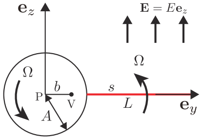
Figure 17: Schematic showing a dielectric particle of radius $A$ connected by a rigid rod of length $L$ and radius $a$. Under a sufficient strong electric field $\mathbf{E}=E\mathbf{e}_{z}$, the composite object rotates about a pivot V that lies on the centreline of rod.

Now we adapt the above derivation to the composite particle-rod system steadily rotating at velocity $\boldsymbol{\Omega}=\Omega\mathbf{e}_{x}$ about an off-centre pivot point V on the $y$-axis (see figure 17). We choose the particle centre P as the origin of the Cartesian coordinates. Using the local SBT, the force per unit length $-\mathbf{f}_{\mathrm{rod}}$ exerted by the fluid onto the rod at arclength $s$ is

$$-\mathbf{f}_{\mathrm{rod}}(s)=-\xi_{\perp}\Omega\left(A-b+s\right)\mathbf{e}_{z},$$ (74)

where $\xi_{\perp}=-8\pi\mu/c=-8\pi\mu/(1+2\log{\epsilon_{\mathrm{sl}}})$, and the total hydrodynamic force $\mathbf{F}_{\mathrm{rod}}$ exerted on the rod is

$$\mathbf{F}_{\mathrm{rod}}=\int_{0}^{L}-\mathbf{f}_{\mathrm{rod}}(s)\mathrm{d}s=-\xi_{\perp}\Omega\left[(A-b)L+L^{2}/2\right]\mathbf{e}_{z}.$$ (75)

Simultaneously, the hydrodynamic force exerted on the translating spherical particle is $\mathbf{F}_{\mathrm{par}}=6\pi\mu Ab\Omega\mathbf{e}_{z}$. Using the force-free condition $\mathbf{F}_{\mathrm{rod}}+\mathbf{F}_{\mathrm{par}}=\mathbf{0}$, we obtain

$$b=\frac{\xi_{\perp}L\left(1+2\alpha\right)}{2\left(6\pi\mu\alpha+\xi_{\perp}\right)}.$$ (76)

The hydrodynamic torque $\boldsymbol{\Gamma}^{\mathrm{hydro}}_{\mathrm{rod}}$ exerted on the rod with respect to the particle centre P is

$$\boldsymbol{\Gamma}^{\mathrm{hydro}}_{\mathrm{rod}} =\int_{0}^{L}(A+s)\mathbf{e}_{y}\times\left[-\xi_{\perp}\Omega\left(A-b+s\right)\mathbf{e}_{z}\right]\mathrm{d}s$$

$$=-\xi_{\perp}\Omega\mathbf{e}_{x}\int_{0}^{L}\left(A+s\right)\left(A-b+s\right)\mathrm{d}s$$

$$=-\frac{\xi_{\perp}\Omega\mathbf{e}_{z}}{6}\left[6\left(A^{2}-Ab\right)L+3\left(2A-b\right)L^{2}+2L^{3}\right].$$ (77)

Using the torque-free condition on the particle-rod system, $\boldsymbol{\Gamma}^{\mathrm{elec}}+\boldsymbol{\Gamma}^{\mathrm{hydro}}_{\mathrm{par}}+\boldsymbol{\Gamma}^{\mathrm{hydro}}_{\mathrm{rod}}=\mathbf{0}$, we obtain

$$\frac{\boldsymbol{\Gamma}^{\mathrm{elec}}+\boldsymbol{\Gamma}^{\mathrm{hydro}}_{\mathrm{par}}+\boldsymbol{\Gamma}^{\mathrm{hydro}}_{\mathrm{rod}}}{2\pi A^{3}\Omega\mathbf{e}_{x}}=\frac{3\epsilon_{\mathrm{s}}E^{2}\left(1-R/S\right)\tau_{\mathrm{MW}}}{\left(1+\frac{2}{S}\right)\left(1+\frac{R}{2}\right)\left(1+\Omega^{2}{(\tau_{\mathrm{MW}})}^{2}\right)}-4\mu\left[1+F\left(\alpha,\hat{\beta},\epsilon_{\mathrm{sl}}\right)\right],$$ (78)

where

$$F\left(\alpha,\hat{\beta},\epsilon_{\mathrm{sl}}\right) =\frac{6\alpha^{-1}\left(1-\hat{\beta}^{-1}\right)+3\alpha^{-2}\left(2-\hat{\beta}^{-1}\right)+2\alpha^{-3}}{6\left(-1-2\log{\epsilon}\right)},$$ (79a)

$$\hat{\beta}=A/b =\frac{2\alpha}{4\left(2\alpha+1\right)}\left[4-3\alpha\left(1+2\log{\epsilon_{\mathrm{sl}}}\right)\right].$$ (79b)

Hence, the critical electrical field corresponding to the instability inception is

$$\bar{\mathcal{E}}^{\mathrm{cri}}=\mathcal{E}^{\mathrm{cri}}/E^{\mathrm{cri}}=\sqrt{1+F}.$$ (80)

The typical values of $\bar{\mathcal{E}}^{\mathrm{cri}}$ as a function of size ratio $\alpha=A/L$ for $\epsilon_{\mathrm{sl}}=0.01$ are provided in table 2.

$\alpha$	0.1	0.3	0.5	0.7	0.9
$\bar{\mathcal{E}}^{\mathrm{cri}}$	5.278	1.803	1.348	1.202	1.136

Table 2: Dimensionless critical electric field $\bar{\mathcal{E}}^{\mathrm{cri}}$ above which the composite object of a dielectric sphere of size ratio $\alpha$ and a rigid rod undergoes the electrohydrodynamic instability, the slenderness $\epsilon_{\mathrm{sl}}=0.01$.

Appendix C Two-dimensional polynomial equations for $\hat{\sigma}_{r}$ and $W$

We substitute equations (47) and (48) into equation (46). We define $E^{\prime}=E^{2}-1$ and $\upsilon=\left(\frac{1}{-1-2\log{\epsilon_{\mathrm{sl}}}}\right)^{1/4}$ that leads to $\log\xi=z_{0}\upsilon W$. Consequently, the system of two-dimensional polynomial equations for $\hat{\sigma}_{r}$ and $W$ reads,

$$\begin{split}&0=-9\hat{\sigma}_{r}^{2}W^{8}\alpha^{5}-24\hat{\sigma}^{2}W^{7}\alpha^{3}\upsilon^{3}\left(\cos\frac{3\pi}{8}+\sin\frac{3\pi}{8}\right)-32\hat{\sigma}_{r}^{2}W^{6}\alpha^{3}\upsilon^{6}\sin\frac{3\pi}{4}\\ &-57\hat{\sigma}_{r}W^{11}\alpha^{4}\upsilon^{3}\left(-\cos\frac{3\pi}{8}+\sin\frac{3\pi}{8}\right)-2\hat{\sigma}W^{10}\alpha^{3}\upsilon^{2}\left(-44\upsilon^{4}\cos{\frac{3\pi}{4}}+9\sin\frac{\pi}{4}\right)\\ &-3\hat{\sigma}_{r}W^{9}\alpha^{2}\upsilon\left[3\cos{\frac{\pi}{8}}+3\sin{\frac{\pi}{8}}+8\upsilon^{4}\left(-\cos{\frac{5\pi}{8}}+\sin{\frac{5\pi}{8}}\right)\right]+9\hat{\sigma}_{r}W^{8}\alpha\left(-4\upsilon^{4}+\kappa\bar{\mu}\alpha^{4}E^{\prime}\right)\\ &+8\hat{\sigma}_{r}W^{7}\upsilon^{3}\left[2\upsilon^{4}\left(\cos{\frac{7\pi}{8}}-\sin{\frac{7\pi}{8}}\right)+3\kappa\bar{\mu}\alpha^{4}E^{\prime}\left(\cos{\frac{3\pi}{8}}+\sin{\frac{3\pi}{8}}\right)\right]+32\kappa\bar{\mu}\hat{\sigma}_{r}W^{6}\alpha^{3}\upsilon^{6}\sin{\frac{3\pi}{4}}E^{\prime}\\ &+9W^{16}\alpha^{5}+33W^{15}\alpha^{4}\upsilon^{3}\left(\cos{\frac{3\pi}{8}}+\sin{\frac{3\pi}{8}}\right)+2W^{14}\alpha^{3}\upsilon^{2}\left(9\cos{\frac{\pi}{4}}+28\upsilon^{4}\sin{\frac{3\pi}{4}}\right)\\ &+3W^{13}\alpha^{2}\upsilon\left[3\cos{\frac{\pi}{8}}-3\sin{\frac{\pi}{8}}+8\upsilon^{4}\left(\cos{\frac{5\pi}{8}}+\sin{\frac{5\pi}{8}}\right)\right]\\ &+W^{11}\upsilon^{3}\left[9\kappa\bar{\mu}\alpha^{4}\left(\cos{\frac{3\pi}{8}}-\sin{\frac{3\pi}{8}}\right)+16\upsilon^{4}\left(\cos{\frac{7\pi}{8}}+\sin{\frac{7\pi}{8}}\right)-24\kappa\bar{\mu}\alpha^{4}E^{\prime}\left(\cos{\frac{3\pi}{8}}-\sin{\frac{3\pi}{8}}\right)\right]\\ &-2\kappa\bar{\mu}W^{10}\alpha^{3}\upsilon^{2}\left(-12\upsilon^{4}\cos{\frac{3\pi}{4}}+9\sin{\frac{\pi}{4}}+16\upsilon^{4}E^{\prime}\cos{\frac{3\pi}{4}}\right)\\ &+3\kappa\bar{\mu}W^{9}\alpha^{2}\upsilon\left[-3\left(\cos{\frac{\pi}{8}}+\sin{\frac{\pi}{8}}\right)+8\upsilon^{4}\left(\cos{\frac{5\pi}{8}}-\sin{\frac{5\pi}{8}}\right)\right]\\ &-36\kappa\bar{\mu}W^{8}\alpha\upsilon^{4}+16\kappa\bar{\mu}W^{7}\upsilon^{7}\left(\cos{\frac{7\pi}{8}}-\sin{\frac{7\pi}{8}}\right),\end{split}$$ (81)

and

$$\begin{split}&0=-24\hat{\sigma}^{2}W^{7}\alpha^{4}\upsilon^{3}\left(\cos{\frac{3\pi}{8}}-\sin{\frac{3\pi}{8}}\right)-32\hat{\sigma}^{2}W^{6}\alpha^{3}\upsilon^{6}\cos{\frac{3\pi}{4}}-18\hat{\sigma}W^{12}\alpha^{5}\\ &-57\hat{\sigma}W^{11}\alpha^{4}\upsilon^{3}\left(\cos{\frac{3\pi}{8}}+\sin{\frac{3\pi}{8}}\right)-2\hat{\sigma}W^{10}\alpha^{3}\upsilon^{2}\left(9\cos\frac{\pi}{4}+44\upsilon^{4}\sin{\frac{3\pi}{4}}\right)\\ &-3\hat{\sigma}W^{9}\alpha^{2}\upsilon\left[3\left(\cos{\frac{\pi}{8}}-\sin{\frac{\pi}{8}}\right)+8\upsilon^{4}\left(\cos{\frac{5\pi}{8}}+\sin{\frac{5\pi}{8}}\right)\right]\\ &-8\hat{\sigma}_{r}W^{7}\upsilon^{3}\left[2\upsilon^{4}\left(\cos{\frac{7\pi}{8}}+\sin{\frac{7\pi}{8}}\right)-3\kappa\bar{\mu}\alpha^{4}E^{\prime}\left(\cos{\frac{3\pi}{8}}-\sin{\frac{3\pi}{8}}\right)\right]+32\kappa\bar{\mu}\hat{\sigma}_{r}W^{6}\alpha^{3}\upsilon^{6}E^{\prime}\cos{\frac{3\pi}{4}}\\ &+33W^{15}\alpha^{4}\upsilon^{3}\left(\cos{\frac{3\pi}{8}}-\sin{\frac{3\pi}{8}}\right)+2W^{14}\alpha^{3}\upsilon^{2}\left(28\upsilon^{4}\cos{\frac{3\pi}{4}}-9\sin\frac{\pi}{4}\right)\\ &+3W^{13}\alpha^{2}\upsilon\left[-3\left(\cos{\frac{\pi}{8}}+\sin{\frac{\pi}{8}}\right)+8\upsilon^{4}\left(\cos{\frac{5\pi}{8}}-\sin{\frac{5\pi}{8}}\right)\right]+9W^{12}\alpha\left(-4\upsilon^{4}+\kappa\bar{\mu}\alpha^{4}E^{\prime}\right)\\ &+W^{11}\upsilon^{3}\left[-9\kappa\bar{\mu}\alpha^{4}\left(\cos{\frac{3\pi}{8}}+\sin{\frac{3\pi}{8}}\right)+16\upsilon^{4}\left(\cos{\frac{7\pi}{8}}-\sin{\frac{7\pi}{8}}\right)+24\kappa\bar{\mu}\alpha^{4}E^{\prime}\left(\cos{\frac{3\pi}{8}}+\sin{\frac{3\pi}{8}}\right)\right]\\ &+2\kappa\bar{\mu}W^{10}\alpha^{3}\upsilon^{2}\left(-9\cos{\frac{\pi}{4}}-12\upsilon^{4}\sin\frac{3\pi}{4}+16\upsilon^{4}E^{\prime}\sin{\frac{3\pi}{4}}\right)\\ &-3\kappa\bar{\mu}W^{9}\alpha^{2}\upsilon\left[3\left(\cos{\frac{\pi}{8}}-\sin{\frac{\pi}{8}}\right)+8\upsilon^{4}\left(\cos{\frac{5\pi}{8}}+\sin{\frac{5\pi}{8}}\right)\right]-16\kappa\bar{\mu}W^{7}\upsilon^{7}\left(\cos{\frac{7\pi}{8}}+\sin{\frac{7\pi}{8}}\right).\end{split}$$ (82)

Appendix D LSA for the minimal model

We perform LSA for the minimal model. Similar to § 4.1, the bars over the dimensionless unknown variables are dropped, unless otherwise specified. The state variables $[\theta,\theta_{1},U_{y},U_{z},\mathcal{P}_{Q},\mathcal{P}_{3}]$ are decomposed into a base state $[\hat{\theta},\hat{\theta}_{1},\hat{U}_{y},\hat{U}_{z},\hat{\mathcal{P}}_{Q},\hat{\mathcal{P}}_{3}]$ and a perturbation state $[\theta^{\prime},\theta_{1}^{\prime},U_{y}^{\prime},U_{z}^{\prime},\mathcal{P}^{\prime}_{Q},\mathcal{P}^{\prime}_{3}]$, where $\hat{\theta}_{1}=\hat{U}_{y}=\hat{U}_{z}=0$, $\hat{\theta}$ is an arbitrary value, and $\hat{\mathcal{P}}_{Q}$ and $\hat{\mathcal{P}}_{3}$ are given by equation (26). By linearising equations (57) and (58) with respect to the base state, we derive the linear evolution equations for the perturbative state variables,

$$(8\alpha+4)\frac{\mathrm{d}\theta^{\prime}}{\mathrm{d}t}\cos\hat{\theta}+\frac{\mathrm{d}\theta_{1}^{\prime}}{\mathrm{d}t}\cos\hat{\theta}+2\left(3-3\alpha c+\cos 2\hat{\theta}\right)U_{y}^{\prime}+2U_{z}^{\prime}\sin 2\hat{\theta} =0,$$

$$(8\alpha+4)\frac{\mathrm{d}\theta^{\prime}}{\mathrm{d}t}\sin\hat{\theta}+\frac{\mathrm{d}\theta_{1}^{\prime}}{\mathrm{d}t}\sin\hat{\theta}+2\left(3-3\alpha c-\cos 2\hat{\theta}\right)U_{z}^{\prime}+2U_{y}^{\prime}\sin 2\hat{\theta} =0,$$

$$\left(3\alpha+5/2\right)\bar{\mu}\frac{\mathrm{d}\theta^{\prime}}{\mathrm{d}t}+\bar{\mu}\frac{\mathrm{d}\theta_{1}^{\prime}}{\mathrm{d}t}+3\bar{\mu}U_{y}^{\prime}\cos\hat{\theta}+3\bar{\mu}U_{z}^{\prime}\sin\hat{\theta}-24c\theta_{1}^{\prime} =0,$$

$$\left(24\alpha^{2}+21\alpha+11/2\right)\bar{\mu}\frac{\mathrm{d}\theta^{\prime}}{\mathrm{d}t}+3\left(\alpha+1/2\right)\bar{\mu}\frac{\mathrm{d}\theta_{1}^{\prime}}{\mathrm{d}t}+\left(24\alpha+9\right)\bar{\mu}\left(U_{y}^{\prime}\cos\hat{\theta}+U_{z}^{\prime}\sin\hat{\theta}\right)$$

$$+24c\theta_{1}^{\prime}-24c\bar{\eta}\frac{\mathrm{d}\theta^{\prime}}{\mathrm{d}t}+24c\bar{\eta}\kappa\bar{E}^{2}\theta^{\prime}+24c\bar{E}\mathcal{P}^{\prime}_{Q}\cos\hat{\theta}-24c\bar{E}\mathcal{P}^{\prime}_{3}\sin\hat{\theta} =0$$

$$\frac{\partial\mathcal{P}^{\prime}_{Q}}{\partial t}+\kappa\mathcal{P}^{\prime}_{Q}+\kappa^{2}\bar{\eta}\bar{E}\theta^{\prime}\cos\hat{\theta} =0,$$

$$\frac{\partial\mathcal{P}^{\prime}_{3}}{\partial t}+\kappa\mathcal{P}^{\prime}_{3}-\kappa^{2}\bar{\eta}\bar{E}\theta^{\prime}\sin\hat{\theta} =0.$$ (83)

Employing the normal-mode approach as in § 4, we substitute $\left[\theta^{\prime},\theta_{1}^{\prime},U_{y}^{\prime},U_{z}^{\prime},\mathcal{P}^{\prime}_{Q},\mathcal{P}^{\prime}_{3}\right]=\left[\Theta,\Theta_{1},\mathcal{Y},\mathcal{Z},\Phi,\Pi\right]\exp{(\sigma t)}$ into equation (D) and derive

$$\left(8\alpha+4\right)\sigma\Theta\cos\hat{\theta}+\sigma\Theta_{1}\cos\hat{\theta}+2\left(3-3\alpha c+\cos 2\hat{\theta}\right)\mathcal{Y}+2\mathcal{Z}\sin 2\hat{\theta} =0,$$

$$\left(8\alpha+4\right)\sigma\Theta\sin\hat{\theta}+\sigma\Theta_{1}\sin\hat{\theta}+2\left(3-3\alpha c-\cos 2\hat{\theta}\right)\mathcal{Z}+2\mathcal{Y}\sin 2\hat{\theta} =0,$$

$$\left(3\alpha+5/2\right)\bar{\mu}\sigma\Theta+\bar{\mu}\sigma\Theta_{1}+3\bar{\mu}\mathcal{Y}\cos\hat{\theta}+3\bar{\mu}\mathcal{Z}\sin\hat{\theta}-24c\Theta_{1} =0,$$

$$\left(24\alpha^{2}+21\alpha+11/2\right)\bar{\mu}\sigma\Theta+3\left(\alpha+1/2\right)\bar{\mu}\sigma\Theta_{1}+(24\alpha+9)\bar{\mu}\left(\mathcal{Y}\cos\hat{\theta}+\mathcal{Z}\sin\hat{\theta}\right)$$

$$+24c\Theta_{1}-24c\bar{\eta}\sigma\Theta+24c\bar{\eta}\kappa\bar{E}^{2}\Theta+24c\bar{E}\left(\Phi\cos\hat{\theta}-\Pi\sin\hat{\theta}\right) =0,$$

$$\left(\sigma+\kappa\right)\Phi+\kappa^{2}\bar{\eta}\bar{E}\Theta\cos\hat{\theta} =0,$$

$$\left(\sigma+\kappa\right)\Pi-\kappa^{2}\bar{\eta}\bar{E}\Theta\sin\hat{\theta} =0.$$ (84)

Setting the determinant of the operator matrix of equation (D) to zero, we find the non-zero solutions of the complex growth rate $\sigma$

$$\sigma_{\pm}=\left\{\pm\sqrt{\Sigma}-6912\alpha c^{3}\bar{\eta}+288c^{2}\left\{\alpha\bar{\mu}\left[\kappa\bar{\eta}+24\alpha(\alpha+1)+8\right]-\alpha\kappa\bar{E}^{2}\bar{\eta}\bar{\mu}+32\bar{\eta}\right\}-3c\bar{\mu}\left\{\alpha\left[12\alpha(5\alpha+3)+7\right]\kappa\bar{\mu}-80\kappa\bar{E}^{2}\bar{\eta}+80\kappa\bar{\eta}+256\right\}+4\kappa\bar{\mu}^{2}\right\}\\ /\left\{48c\bar{\eta}(5-6\alpha c)+\bar{\mu}\left[3\alpha(12\alpha(5\alpha+3)+7\right]c-4)\right\},$$ (85)

where

$$\scriptsize\Sigma=\left\{2304c^{2}\bar{\eta}(3\alpha c-4)-48c\bar{\mu}\left[6\alpha c\left(\kappa\bar{\eta}+24\alpha(\alpha+1)+8\right)-5\kappa\bar{\eta}-16\right]+\kappa\bar{\mu}^{2}\left[3\alpha(12\alpha(5\alpha+3)+7)c-4\right]+48c\kappa\bar{E}^{2}\bar{\eta}\bar{\mu}(6\alpha c-5)\right\}^{2}-3072c\kappa\bar{\mu}\left\{48c\bar{\eta}(6\alpha c-5)-3\alpha\left[12\alpha(5\alpha+3)+7\right]c\bar{\mu}+4\bar{\mu}\right\}\left\{3c\bar{\eta}(4-3\alpha c)+\bar{\mu}\left[3\alpha(3\alpha(\alpha+1)+1)c-1\right]+3c\bar{E}^{2}\bar{\eta}(3\alpha c-4)\right\}.$$ (86)

We plot $\sigma_{r}$ and $\sigma_{i}$ in comparison with their numerical counterparts in figure 16.

References

- Alapan et al. (2019) Alapan, Y., Yasa, O., Yigit, B., Yasa, I. C., Erkoc, P. & Sitti, M. 2019 Microrobotics and microorganisms: Biohybrid autonomous cellular robots. Annu. Rev. Control Rob. Auton. Syst. 2, 205–230.
- Batchelor (1970) Batchelor, G. K. 1970 Slender-body theory for particles of arbitrary cross-section in Stokes flow. J. Fluid Mech. 44 (3), 419–440.
- Bayly & Dutcher (2016) Bayly, P. V. & Dutcher, S. K. 2016 Steady dynein forces induce flutter instability and propagating waves in mathematical models of flagella. J. R. Soc. Interface 13 (123), 20160523.
- Bigoni et al. (2018) Bigoni, D., Kirillov, O. N., Misseroni, D., Noselli, G. & Tommasini, M. 2018 Flutter and divergence instability in the Pflüger column: Experimental evidence of the Ziegler destabilization paradox. J. Mech. Phys. Solids 116, 99–116.
- Bricard et al. (2013) Bricard, A., Caussin, J. B., Desreumaux, N. & Bartolo, O. Dauchotand D. 2013 Emergence of macroscopic directed motion in populations of motile colloids. Nature 503 (7474), 95–98.
- Brokaw (1971) Brokaw, C. J. 1971 Bend propagation by a sliding filament model for flagella. J. Exp. Biol. 55 (2), 289–304.
- Brokaw (2009) Brokaw, C. J. 2009 Thinking about flagellar oscillation. Cell Motil. Cytoskeleton 66 (8), 425–436.
- Brosseau et al. (2017) Brosseau, Q., Hickey, G. & Vlahovska, P. M. 2017 Electrohydrodynamic Quincke rotation of a prolate ellipsoid. Phys. Rev. Fluids 2 (1), 014101.
- Cates & MacKintosh (2011) Cates, M. E. & MacKintosh, F. C. 2011 Active soft matter. Soft Matter 7 (7), 3050–3051.
- Cēbers et al. (2000) Cēbers, A., Lemaire, E. & Lobry, L. 2000 Electrohydrodynamic instabilities and orientation of dielectric ellipsoids in low-conducting fluids. Phys. Rev. E 63 (1), 016301.
- Coq et al. (2008) Coq, N., du Roure, O., Marthelot, J., Bartolo, D. & Fermigier, M. 2008 Rotational dynamics of a soft filament: Wrapping transition and propulsive forces. Phys. Fluids 20 (5), 051703.
- Das & Lauga (2019) Das, D. & Lauga, E. 2019 Active particles powered by Quincke rotation in a bulk fluid. Phys. Rev. Lett. 122 (19), 194503.
- Das & Saintillan (2013) Das, D. & Saintillan, D. 2013 Electrohydrodynamic interaction of spherical particles under Quincke rotation. Phys. Rev. E 87 (4), 043014.
- De Canio et al. (2017) De Canio, G., Lauga, E. & Goldstein, R. E. 2017 Spontaneous oscillations of elastic filaments induced by molecular motors. J. R. Soc. Interface 14 (136), 20170491.
- Dreyfus et al. (2005) Dreyfus, R., Baudry, J., Roper, M. L., Fermigier, M., Stone, H. A. & Bibette, J. 2005 Microscopic artificial swimmers. Nature 437 (7060), 862.
- Evans et al. (2007) Evans, B. A., Shields, A. R., Carroll, R. L., Washburn, S., Falvo, M. R. & Superfine, R. 2007 Magnetically actuated nanorod arrays as biomimetic cilia. Nano Lett. 7 (5), 1428–1434.
- Fatehiboroujeni et al. (2018) Fatehiboroujeni, S., Gopinath, A. & Goyal, S. 2018 Nonlinear oscillations induced by follower forces in prestressed clamped rods subjected to drag. J. Comput. Nonlinear Dyn. 13 (12), 121005.
- Fawcett (1961) Fawcett, D. 1961 Cilia and flagella. In The Cell: Biochemistry, Physiology, Morphology (ed. J. Brachet & A. E. Mirsky), , vol. 2, pp. 217–297. Elsevier.
- Gold (1948) Gold, T. 1948 Hearing. II. the physical basis of the action of the cochlea. Proc. R. Soc. London, Ser. B 135 (881), 492–498.
- Guglielmini et al. (2012) Guglielmini, L., Kushwaha, A., Shaqfeh, E. S. G. & Stone, H. A. 2012 Buckling transitions of an elastic filament in a viscous stagnation point flow. Phys. Fluids 24 (12), 123601.
- Hanasoge et al. (2017) Hanasoge, S., Ballard, M., Hesketh, P. J. & Alexeev, A. 2017 Asymmetric motion of magnetically actuated artificial cilia. Lab Chip 17 (18), 3138–3145.
- Herrmann & Bungay (1964) Herrmann, G. & Bungay, R. W. 1964 On the stability of elastic systems subjected to nonconservative forces. J. Appl. Mech. 31 (3), 435–440.
- Hilfinger et al. (2009) Hilfinger, A., Chattopadhyay, A. K. & Jülicher, F. 2009 Nonlinear dynamics of cilia and flagella. Phys. Rev. E 79 (5), 051918.
- Hines & Blum (1983) Hines, M. & Blum, J. J. 1983 Three-dimensional mechanics of eukaryotic flagella. Biophys. J. 41 (1), 67.
- Hu & Bayly (2018) Hu, T. & Bayly, P. V. 2018 Finite element models of flagella with sliding radial spokes and interdoublet links exhibit propagating waves under steady dynein loading. Cytoskeleton 75 (5), 185–200.
- Huang et al. (2019) Huang, H-W, Uslu, F. E., Katsamba, P., Lauga, E., Sakar, M. S. & Nelson, B. J. 2019 Adaptive locomotion of artificial microswimmers. Sci. Adv. 5 (1), eaau1532.
- Jenkins (2013) Jenkins, A. 2013 Self-oscillation. Phys. Rep. 525 (2), 167–222.
- Jones (1984) Jones, T. B. 1984 Quincke rotation of spheres. IEEE Trans. Ind. Appl. IA–20 (4), 845–849.
- Kemp (1979) Kemp, D. T. 1979 Evidence of mechanical nonlinearity and frequency selective wave amplification in the cochlea. Arch. Otorhinolaryngol. 224 (1-2), 37–45.
- Kieseok et al. (2009) Kieseok, O., Chung, J.-H., Devasia, S. & Riley, J. J. 2009 Bio-mimetic silicone cilia for microfluidic manipulation. Lab Chip 9 (11), 1561–1566.
- Koiter (1996) Koiter, W. T. 1996 Unrealistic follower forces. J. Sound Vib. 194, 636–636.
- Lauga & Powers (2009) Lauga, E. & Powers, T. 2009 The hydrodynamics of swimming microorganisms. Rep. Prog. Phys. 72, 096601.
- Li et al. (2013) Li, L., Manikantan, H., Saintillan, D. & Spagnolie, S. E. 2013 The sedimentation of flexible filaments. J. Fluid Mech. 735, 705–736.
- Ling et al. (2018) Ling, F., Guo, H. & Kanso, E. 2018 Instability-driven oscillations of elastic microfilaments. J. R. Soc. Interface 15 (149), 20180594.
- Livanovičs & Cēbers (2012) Livanovičs, R. & Cēbers, A. 2012 Magnetic dipole with a flexible tail as a self-propelling microdevice. Phys. Rev. E 85 (4), 041502.
- Manghi et al. (2006) Manghi, M., Schlagberger, X. & Netz, R. R. 2006 Propulsion with a rotating elastic nanorod. Phys. Rev. Lett. 96 (6), 068101.
- Marchetti et al. (2013) Marchetti, M. C., Joanny, J. F., Ramaswamy, S., Liverpool, T. B., Prost, J., Rao, M. & Simha, R. A. 2013 Hydrodynamics of soft active matter. Rev. Mod. Phys. 85 (3), 1143.
- Masuda et al. (2013) Masuda, T., Hidaka, M., Murase, Y., Akimoto, A. M., Nagase, K., Okano, T. & Yoshida, R. 2013 Self-oscillating polymer brushes. Angew. Chem. 125 (29), 7616–7619.
- Needleman & Dogic (2017) Needleman, D. & Dogic, Z. 2017 Active matter at the interface between materials science and cell biology. Nat. Rev. Mater. 2 (9), 17048.
- van Oosten et al. (2009) van Oosten, C. L., Bastiaansen, C. W. M. & Broer, D. J. 2009 Printed artificial cilia from liquid-crystal network actuators modularly driven by light. Nat. Mater. 8 (8), 677.
- Otto et al. (2019) Otto, J., Forbes, A. & Verschelde, J. 2019 Solving polynomial systems with phcpy. arXiv preprint arXiv:1907.00096 .
- Peters et al. (2005) Peters, F., Lobry, L. & Lemaire, E. 2005 Experimental observation of Lorenz chaos in the Quincke rotor dynamics. Chaos 15 (1), 013102.
- Pflüger (1950) Pflüger, A. 1950 Stabilitätsprobleme der Elastostatik. Springer-Verlag.
- Qian et al. (2008) Qian, B., Powers, T. R. & Breuer, K. S. 2008 Shape transition and propulsive force of an elastic rod rotating in a viscous fluid. Phys. Rev. Lett. 100 (7), 078101.
- Quincke (1896) Quincke, G. 1896 Ueber rotationen im constanten electrischen felde. Ann. Phys. 295 (11), 417–486.
- Ramaswamy (2010) Ramaswamy, S. 2010 The mechanics and statistics of active matter. Annu. Rev. Condens. Matter Phys. 1 (1), 323–345.
- Riedel-Kruse et al. (2007) Riedel-Kruse, I. H., Müller, C. & Oates, A. C. 2007 Synchrony dynamics during initiation, failure, and rescue of the segmentation clock. Science 317 (5846), 1911–1915.
- Sartori et al. (2016) Sartori, P., Geyer, V. F., Scholich, A., Jülicher, F. & Howard, J. 2016 Dynamic curvature regulation accounts for the symmetric and asymmetric beats of chlamydomonas flagella. Elife 5, e13258.
- Sel’kov (1968) Sel’kov, E. E. 1968 Self-oscillations in glycolysis 1. a simple kinetic model. Eur. J. Biochem. 4 (1), 79–86.
- Sidorenko et al. (2007) Sidorenko, A., Krupenkin, T., Taylor, A., Fratzl, P. & Aizenberg, J. 2007 Reversible switching of hydrogel-actuated nanostructures into complex micropatterns. Science 315 (5811), 487–490.
- Singh et al. (2005) Singh, H., Laibinis, P. E. & Hatton, T. A. 2005 Synthesis of flexible magnetic nanowires of permanently linked core-shell magnetic beads tethered to a glass surface patterned by microcontact printing. Nano Lett. 5 (11), 2149–2154.
- den Toonder et al. (2008) den Toonder, J., Bos, F., Broer, D., Filippini, L., Gillies, M., de Goede, J., Mol, T., Reijme, M., Talen, W., Wilderbeek, H., Khatavkar, V. & Anderson, P. 2008 Artificial cilia for active micro-fluidic mixing. Lab Chip 8 (4), 533–541.
- Tornberg & Shelley (2004) Tornberg, A. K. & Shelley, M. J. 2004 Simulating the dynamics and interactions of flexible fibers in Stokes flows. J. Comput. Phys. 196 (1), 8–40.
- Tsebers (1980a) Tsebers, A. O. 1980a Electrohydrodynamic instabilities in a weakly conducting suspension of ellipsoidal particles. Magnetohydrodynamics 16 (2), 175–180.
- Tsebers (1980b) Tsebers, A. O. 1980b Internal rotation in the hydrodynamics of weakly conducting dielectric suspensions. Fluid Dyn. 15 (2), 245–251.
- Tsebers (1991) Tsebers, A. O. 1991 Chaotic solutions for the relaxation equations of electrical polarization. Magnetohydrodynamics 27 (3), 251–258.
- Turcu (1987) Turcu, I. 1987 Electric field induced rotation of spheres. J. Phys. A: Math. Gen. 20 (11), 3301–3307.
- Verschelde (1997) Verschelde, J. 1997 PHCPACK: A general-purpose solver for polynomial systems by homotopy continuation. Technical Report TW265, Department of Computer Science, Katholieke Universiteit Leuven .
- Verschelde (2013) Verschelde, J. 2013 Modernizing PHCpack through phcpy. arXiv preprint arXiv:1310.0056 .
- Wiggins & Goldstein (1998) Wiggins, C. H. & Goldstein, R. E. 1998 Flexive and propulsive dynamics of elastica at low Reynolds number. Phys. Rev. Lett. 80 (17), 3879–3882.
- Wiggins et al. (1998) Wiggins, C. H., Riveline, D., Ott, A. & Goldstein, R. E. 1998 Trapping and wiggling: elastohydrodynamics of driven microfilaments. Biophys. J. 74 (2), 1043–1060.
- Zaks & Shliomis (2014) Zaks, M. A. & Shliomis, M. I. 2014 Onset and breakdown of relaxation oscillations in the torsional Quincke pendulum. Preprint on webpage at https://www.researchgate.net/publication/267410780_Onset_and_breakdown_of_relaxation_oscillations_in_the_torsional_Quincke_pendulum.
- Zhu & Stone (2019) Zhu, L. & Stone, H. A. 2019 Propulsion driven by self-oscillation via an electrohydrodynamic instability. Phys. Rev. Fluids 4 (6), 061701.
- Ziegler (1952) Ziegler, H. 1952 Die stabilitätskriterien der elastomechanik. Ingenieur-Archiv 20 (1), 49–56.