Reliable training and estimation of variance networks

Abstract

We propose and investigate new complementary methodologies for estimating predictive variance networks in regression neural networks. We derive a locally aware mini-batching scheme that results in sparse robust gradients, and we show how to make unbiased weight updates to a variance network. Further, we formulate a heuristic for robustly fitting both the mean and variance networks post hoc. Finally, we take inspiration from posterior Gaussian processes and propose a network architecture with similar extrapolation properties to Gaussian processes. The proposed methodologies are complementary, and improve upon baseline methods individually. Experimentally, we investigate the impact of predictive uncertainty on multiple datasets and tasks ranging from regression, active learning and generative modeling. Experiments consistently show significant improvements in predictive uncertainty estimation over state-of-the-art methods across tasks and datasets.

1 Introduction

The quality of mean predictions has dramatically increased in the last decade with the rediscovery of neural networks (LeCun et al., 2015). The predictive variance, however, has turned out to be a more elusive target, with established solutions being subpar. The general finding is that neural networks tend to make overconfident predictions (Guo et al., 2017) that can be harmful or offensive (Amodei et al., 2016). This may be explained by neural networks being general function estimators that does not come with principled uncertainty estimates. Another explanation is that variance estimation is a fundamentally different task than mean estimation, and that the tools for mean estimation perhaps do not generalize. We focus on the latter hypothesis within regression.

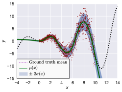
Figure 1: Max. likelihood fit of $\mathcal{N}(\mu(x),\sigma^{2}(x))$ to data.

To illustrate the main practical problems in variance estimation, we consider a toy problem where data is generated as $y=x\cdot\sin(x)+0.3\cdot\epsilon_{1}+0.3\cdot x\cdot\epsilon_{2}$, with $\epsilon_{1},\epsilon_{2}\sim\mathcal{N}(0,1)$ and $x$ is uniform on $[0,10]$ (Fig. 1). As is common, we do maximum likelihood estimation of $\mathcal{N}(\mu(x),\sigma^{2}(x))$, where $\mu$ and $\sigma^{2}$ are neural nets. While $\mu$ provides an almost perfect fit to the ground truth, $\sigma^{2}$ shows two problems: $\sigma^{2}$ is significantly underestimated and $\sigma^{2}$ does not increase outside the data support to capture the poor mean predictions.

These findings are general (Sec. 4), and alleviating them is the main purpose of the present paper. We find that this can be achieved by a combination of methods that 1) change the usual mini-batching to be location aware; 2) only optimize variance conditioned on the mean; 3) for scarce data, we introduce a more robust likelihood function; and 4) enforce well-behaved interpolation and extrapolation of variances. Points 1 and 2 are achieved through changes to the training algorithm, while 3 and 4 are changes to model specifications. We empirically demonstrate that these new tools significantly improve on state-of-the-art across datasets in tasks ranging from regression to active learning, and generative modeling.

2 Related work

Gaussian processes (GPs) are well-known function approximators with built-in uncertainty estimators (Rasmussen and Williams, 2006). GPs are robust in settings with a low amount of data, and can model a rich class of functions with few hyperparameters. However, GPs are computationally intractable for large amounts of data and limited by the expressiveness of a chosen kernel. Advances like sparse and deep GPs (Snelson and Ghahramani, 2006; Damianou and Lawrence, 2013) partially alleviate this, but neural nets still tend to have more accurate mean predictions.

Uncertainty aware neural networks model the predictive mean and variance as two separate neural networks, often as multi-layer perceptrons. This originates with the work of Nix and Weigend (1994) and Bishop (1994); today, the approach is commonly used for making variational approximations (Kingma and Welling, 2013; Rezende et al., 2014), and it is this general approach we investigate.

Bayesian neural networks (BNN) (MacKay, 1992) assume a prior distribution over the network parameters, and approximate the posterior distribution. This gives direct access to the approximate predictive uncertainty. In practice, placing an informative prior over the parameters is non-trivial. Even with advances in stochastic variational inference (Kingma and Welling, 2013; Rezende et al., 2014; Hoffman et al., 2013) and expectation propagation (Hernández-Lobato and Adams, 2015), it is still challenging to perform inference in BNNs.

Ensemble methods represent the current state-of-the-art. Monte Carlo (MC) Dropout (Gal and Ghahramani, 2016) measure the uncertainty induced by Dropout layers (Hinton et al., 2012) arguing that this is a good proxy for predictive uncertainty. Deep Ensembles (Lakshminarayanan et al., 2017) form an ensemble from multiple neural networks trained with different initializations. Both approaches obtain ensembles of correlated networks, and the extent to which this biases the predictive uncertainty is unclear. Alternatives include estimating confidence intervals instead of variances (Pearce et al., 2018), and gradient-based Bayesian model averaging (Maddox et al., 2019).

Applications of uncertainty include reinforcement learning, active learning, and Bayesian optimization (Szepesvári, 2010; Huang et al., 2010; Frazier, 2018). Here, uncertainty is the crucial element that allows for systematically making a trade-off between exploration and exploitation. It has also been shown that uncertainty is required to learn the topology of data manifolds (Hauberg, 2018).

The main categories of uncertainty are epistemic and aleatoric uncertainty (Kiureghian and Ditlevsen, 2009; Kendall and Gal, 2017). Aleatoric uncertainty is induced by unknown or unmeasured features, and, hence, does not vanish in the limit of infinite data. Epistemic uncertainty is often referred to as model uncertainty, as it is the uncertainty due to model limitations. It is this type of uncertainty that Bayesian and ensemble methods generally estimate. We focus on the overall predictive uncertainty, which reflects both epistemic and aleatoric uncertainty.

3 Methods

The opening remarks (Sec. 1) highlighted two common problems that appear when $\mu$ and $\sigma^{2}$ are neural networks. In this section we analyze these problems and propose solutions.

Preliminaries.

We assume that datasets $\mathcal{D}=\{{\boldsymbol{x}}_{i},y_{i}\}_{i=1}^{N}$ contain i.i.d. observations $y_{i}\in\mathbb{R},{\boldsymbol{x}}_{i}\in\mathbb{R}^{D}$. The targets $y_{i}$ are assumed to be conditionally Gaussian, $p_{\theta}(y|{\boldsymbol{x}})=\mathcal{N}(y|\mu({\boldsymbol{x}}),\sigma^{2}({\boldsymbol{x}}))$, where $\mu$ and $\sigma^{2}$ are continuous functions parametrized by $\theta=\{\theta_{\mu},\theta_{\sigma^{2}}\}$. The maximum likelihood estimate (MLE) of the variance of i.i.d. observations $\{y_{i}\}_{i=1}^{N}$ is $\frac{1}{N-1}\sum_{i}(y_{i}-\hat{\mu})^{2}$, where $\hat{\mu}$ is the sample mean. This MLE does not exist based on a single observation, unless the mean $\mu$ is known, i.e. the mean is not a free parameter. When $y_{i}$ is Gaussian, the residuals $(y_{i}-\mu)^{2}$ are gamma distributed.

3.1 A local likelihood model analysis

By assuming that both $\mu$ and $\sigma^{2}$ are continuous functions, we are implicitly saying that $\sigma^{2}({\boldsymbol{x}})$ is correlated with $\sigma^{2}({\boldsymbol{x}}+\delta)$ for sufficiently small $\delta$, and similar for $\mu$. Consider the local likelihood estimation problem (Loader, 1999; Tibshirani and Hastie, 1987) at a point ${\boldsymbol{x}}_{i}$,

$$\log\tilde{p}_{\theta}(y_{i}|{\boldsymbol{x}}_{i})=\sum_{j=1}^{N}w_{j}({\boldsymbol{x}}_{i})\log p_{\theta}(y_{j}|{\boldsymbol{x}}_{j}),$$ (1)

where $w_{j}$ is a function that declines as $\|{\boldsymbol{x}}_{j}-{\boldsymbol{x}}_{i}\|$ increases, implying that the local likelihood at ${\boldsymbol{x}}_{i}$ is dependent on the points nearest to ${\boldsymbol{x}}_{i}$. Notice $\tilde{p}_{\theta}(y_{i}|{\boldsymbol{x}}_{i})=p_{\theta}(y_{i}|{\boldsymbol{x}}_{i})$ if $w_{j}({\boldsymbol{x}}_{i})=\mathbf{1}_{i=j}$. Consider, with this $w$, a uniformly drawn subsample (i.e. a standard mini-batch) of the data $\{{\boldsymbol{x}}_{k}\}_{k=1}^{M}$ and its corresponding stochastic gradient of Eq. 1 with respect to $\theta_{\sigma^{2}}$. If for a point, ${\boldsymbol{x}}_{i}$, no points near it are in the subsample, then no other point will influence the gradient of $\sigma^{2}({\boldsymbol{x}}_{i})$, which will point in the direction of the MLE, that is highly uninformative as it does not exist unless $\mu({\boldsymbol{x}}_{i})$ is known. Local data scarcity, thus, implies that while we have sufficient data for fitting a mean, locally we have insufficient data for fitting a variance. Essentially, if a point is isolated in a mini-batch, all information it carries goes to updating $\mu$ and none is present for $\sigma^{2}$.

If we do not use mini-batches, we encounter that gradients wrt. $\theta_{\mu}$ and $\theta_{\sigma^{2}}$ will both be scaled with $\frac{1}{2\sigma^{2}({\boldsymbol{x}})}$ meaning that points with small variances effectively have higher learning rates (Nix and Weigend, 1994). This implies a bias towards low-noise regions of data.

3.2 Horvitz-Thompson adjusted stochastic gradients

We will now consider a solution to this problem within the local likelihood framework, which will give us a reliable, but biased, stochastic gradient for the usual (nonlocal) log-likelihood. We will then show how this can be turned into an unbiased estimator.

If we are to add some local information, giving more reliable gradients, we should choose a $w$ in Eq.1 that reflects this. Assume for simplicity that $w_{j}({\boldsymbol{x}}_{i})=\textbf{1}_{\|{\boldsymbol{x}}_{i}-{\boldsymbol{x}}_{j}\|<d}$ for some $d>0$. The gradient of $\log\tilde{p}_{\theta}(y|{\boldsymbol{x}}_{i})$ will then be informative, as more than one observation will contribute to the local variance if $d$ is chosen appropriately. Accordingly, we suggest a practical mini-batching algorithm that samples a random point ${\boldsymbol{x}}_{j}$ and we let the mini-batch consist of the $k$ nearest neighbors of ${\boldsymbol{x}}_{j}$. In order to allow for more variability in a mini-batch, we suggest sampling $m$ points uniformly, and then sampling $n$ points among the $k$ nearest neighbors of each of the $m$ initially sampled points. Note that this is a more informative sample, as all observations in the sample are likely to influence the same subset of parameters in $\theta$, effectively increasing the degrees of freedom, hence the quality of variance estimation. In other words, if the variance network is sufficiently expressive, our Monte Carlo gradients under this sampling scheme are of smaller variation and more sparse. In the supplementary material, we empirically show that this estimator yields significantly more sparse gradients, which results in improved convergence. Pseudo-code of this sampling-scheme, can be found in the supplementary material.

While such a mini-batch would give rise to an informative stochastic gradient, it would not be an unbiased stochastic gradient of the (nonlocal) log-likelihood. This can, however, be adjusted by using the Horvitz-Thompson (HT) algorithm (Horvitz and Thompson, 1952), i.e. rescaling the log-likelihood contribution of each sample ${\boldsymbol{x}}_{j}$ by its inclusion probability $\pi_{j}$. With this, an unbiased estimate of the log-likelihood (up to an additive constant) becomes

$$\sum_{i=1}^{N}\left\{-\frac{1}{2}\log(\sigma^{2}({\boldsymbol{x}}_{i}))-\frac{(y_{i}-\mu({\boldsymbol{x}}_{i}))^{2}}{2\sigma^{2}({\boldsymbol{x}}_{i})}\right\}\approx\sum_{{\boldsymbol{x}}_{j}\in\mathcal{O}}\frac{1}{\pi_{j}}\left\{-\frac{1}{2}\log(\sigma^{2}({\boldsymbol{x}}_{j}))-\frac{(y_{j}-\mu({\boldsymbol{x}}_{j}))^{2}}{2\sigma^{2}({\boldsymbol{x}}_{j})}\right\}$$ (2)

where $\mathcal{O}$ denotes the mini-batch. With the nearest neighbor mini-batching, the inclusion probabilities can be calculated as follows. The probability that observation $j$ is in the sample is $\nicefrac{{n}}{{k}}$ if it is among the $k$ nearest neighbors of one of the initial $m$ points, which are chosen with probability $m/N$, i.e.

$$\pi_{j}=\frac{m}{N}\sum_{i=1}^{N}\frac{n}{k}\ \mathbf{1}_{j\in\mathcal{O}_{k}(i)},$$ (3)

where $\mathcal{O}_{k}(i)$ denotes the $k$ nearest neighbors of ${\boldsymbol{x}}_{i}$.

Computational costs

The proposed sampling scheme requires an upfront computational cost of $O(N^{2}D)$ before any training can begin. We stress that this is pre-training computation and not updated during training. The cost is therefore relative small, compared to training a neural network for small to medium size datasets. Additionally, we note that the search algorithm does not have to be precise, and we could therefore take advantage of fast approximate nearest neighbor algorithms (Fu and Cai, 2016).

3.3 Mean-variance split training

The most common training strategy is to first optimize $\theta_{\mu}$ assuming a constant $\sigma^{2}$, and then proceed to optimize $\theta=\{\theta_{\mu},\theta_{\sigma^{2}}\}$ jointly, i.e. a warm-up of $\mu$. As previously noted, the MLE of $\sigma^{2}$ does not exist when only a single observation is available and $\mu$ is unknown. However, the MLE does exist when $\mu$ is known, in which case it is $\hat{\sigma}^{2}({\boldsymbol{x}}_{i})=(y_{i}-\mu({\boldsymbol{x}}_{i}))^{2}$, assuming that the continuity of $\sigma^{2}$ is not crucial. This observation suggests that the usual training strategy is substandard as $\sigma^{2}$ is never optimized assuming $\mu$ is known. This is easily solved: we suggest to never updating $\mu$ and $\sigma^{2}$ simultaneously, i.e. only optimize $\mu$ conditioned on $\sigma^{2}$, and vice versa. This reads as sequentially optimizing $p_{\theta}(y|\theta_{\mu})$ and $p_{\theta}(y|\theta_{\sigma^{2}})$, as we under these conditional distributions we may think of $\mu$ and $\sigma^{2}$ as known, respectively. We will refer to this as mean-variance split training (MV).

3.4 Estimating distributions of variance

When $\sigma^{2}({\boldsymbol{x}}_{i})$ is influenced by few observations, underestimation is still likely due to the left skewness of the gamma distribution of $\hat{\sigma}_{i}^{2}=(y_{i}-\mu({\boldsymbol{x}}_{i}))^{2}$. As always, when in a low data regime, it is sensible to be Bayesian about it; hence instead of point estimating $\hat{\sigma}_{i}^{2}$ we seek to find a distribution. Note that we are not imposing a prior, we are training the parameters of a Bayesian model. We choose the inverse-Gamma distribution, as this is the conjugate prior of $\sigma^{2}$ when data is Gaussian. This means $\theta_{\sigma^{2}}=\{\theta_{\alpha},\theta_{\beta}\}$ where $\alpha,\beta>0$ are the shape and scale parameters of the inverse-Gamma respectively. So the log-likelihood is now calculated by integrating out $\sigma^{2}$

$$\log p_{\theta}(y_{i})=\log\int\mathcal{N}(y_{i}|\mu_{i},\sigma_{i}^{2})\mathrm{d}\sigma_{i}^{2}=\log t_{\mu_{i},\alpha_{i},\beta_{i}}(y_{i}),$$ (4)

where $\sigma_{i}^{2}\sim\textsc{Inv-Gamma}(\alpha_{i},\beta_{i})$ and $\alpha_{i}=\alpha({\boldsymbol{x}}_{i}),\beta_{i}=\beta({\boldsymbol{x}}_{i})$ are modeled as neural networks. Having an inverse-Gamma prior changes the predictive distribution to a located-scaled Student-t distribution, parametrized with $\mu,\alpha$ and $\beta$. Further, the t-distribution is often used as a replacement of the Gaussian when data is scarce and the true variance is unknown and yields a robust regression (Gelman et al., 2014; Lange et al., 1989). We let $\alpha$ and $\beta$ be neural networks that implicitly determine the degrees of freedom and the scaling of the distribution. Recall the higher the degrees of freedom, the better the Gaussian approximation of the $t$-distribution.

3.5 Extrapolation architecture

If we evaluate the local log-likelihood (Eq. 1) at a point ${\boldsymbol{x}}_{0}$ far away from all data points, then the weights $w_{i}({\boldsymbol{x}}_{0})$ will all be near (or exactly) zero. Consequently, the local log-likelihood is approximately 0 regardless of the observed value $y({\boldsymbol{x}}_{0})$, which should be interpreted as a large entropy of $y({\boldsymbol{x}}_{0})$. Since we are working with Gaussian and t-distributed variables, we can recreate this behavior by exploiting the fact that entropy is only an increasing function of the variance. We can re-enact this behavior by letting the variance tend towards an a priori determined value $\eta$ if ${\boldsymbol{x}}_{0}$ tends away from the training data. Let $\{\mathbf{c}_{i}\}_{i=1}^{L}$ be points in $\mathbb{R}^{D}$ that represent the training data, akin to inducing points in sparse GPs (Snelson and Ghahramani, 2006). Then define $\delta({\boldsymbol{x}}_{0})=\min_{i}\|\mathbf{c}_{i}-{\boldsymbol{x}}_{0}\|$ and

$$\hat{\sigma}^{2}({\boldsymbol{x}}_{0})=\big{(}1-\nu(\delta({\boldsymbol{x}}_{0}))\big{)}\hat{\sigma}^{2}_{\theta}+\eta\nu(\delta({\boldsymbol{x}}_{0})),$$ (5)

where $\nu:[0,\infty)\mapsto[0,1]$ is a surjectively increasing function. Then the variance estimate will go to $\eta$ as $\delta\rightarrow\infty$ at a rate determined by $\nu$. In practice, we choose $\nu$ to be a scaled-and-translated sigmoid function: $\nu(x)=\text{sigmoid}((x+a)/\gamma)$, where $\gamma$ is a free parameter we optimize during training and $a\approx-6.9077\gamma$ to ensure that $\nu(0)\approx 0$. The inducing points $\mathbf{c}_{i}$ are initialized with $k$-means and optimized during training. This choice of architecture is similar to that attained by posterior Gaussian processes when the associated covariance function is stationary. It is indeed the behavior of these established models that we aim to mimic with Eq. 5.

4 Experiments

4.1 Regression

To test our methodologies we conduct multiple experiments in various settings. We compare our method to state-of-the-art methods for quantifying uncertainty: Bayesian neural network (BNN) (Hernández-Lobato and Adams, 2015), Monte Carlo Dropout (MC-Dropout) (Gal and Ghahramani, 2016) and Deep Ensembles (Ens-NN) (Lakshminarayanan et al., 2017). Additionally we compare to two baseline methods: standard mean-variance neural network (NN) (Nix and Weigend, 1994) and GPs (sparse GPs (SGP) when standard GPs are not applicable) (Rasmussen and Williams, 2006). We refer to our own method(s) as Combined, since we apply all the methodologies described in Sec. 3. Implementation details and code can be found in the supplementary material. Strict comparisons of the models should be carefully considered; having two seperate networks to model mean and variance seperately (as NN, Ens-NN and Combined) means that all the predictive uncertainty, i.e. both aleatoric and episteminc, is modeled by the variance networks alone. BNN and MC-Dropout have a higher emphasis on modeling epistemic uncertainty, while GPs have the cleanest separation of noise and model uncertainty estimation. Despite the methods quantifying different types of uncertainty, their results can still be ranked by test set log-likelihood, which is a proper scoring function.

Toy regression.

We first return to the toy problem of Sec. 1, where we consider 500 points from $y={\boldsymbol{x}}\cdot\sin({\boldsymbol{x}})+0.3\cdot\epsilon_{1}+0.3\cdot{\boldsymbol{x}}\cdot\epsilon_{2}$, with $\epsilon_{1},\epsilon_{2}\sim\mathcal{N}(0,1)$. In this example, the variance is heteroscedastic, and models should estimate larger variance for larger values of ${\boldsymbol{x}}$. The results can be seen in Figs.  4.1 and 2a. Our approach is the only one to satisfy all of the following: capture the heteroscedasticity, extrapolate high variance outside data region and not underestimating within.

figureFrom top left to bottom right: GP, NN,

BNN, MC-Dropout, Ens-NN, Combined.

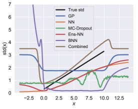
(a)

figureStandard deviation estimates as a function of ${\boldsymbol{x}}$.

Variance calibration.

To our knowledge, no benchmark for quantifying variance estimation exists. We propose a simple dataset with known uncertainty information. More precisely, we consider weather data from over 130 years. Each day the maximum temperature is measured, and the uncertainty is then given as the variance in temperature over the 130 years. The fitted models can be seen in Fig. 2. Here we measure performance by calculating the mean error in uncertainty: $\text{Err}=\frac{1}{N}\sum_{i=1}^{N}|\sigma^{2}_{\text{true}}({\boldsymbol{x}}_{i})-\sigma^{2}_{\text{est}}({\boldsymbol{x}}_{i})|$. The numbers are reported above each fit. We observe that our Combined model achieves the lowest error of all the models, closely followed by Ens-NN and GP. Both NN, BNN and MC-Dropout all severely underestimate the uncertainty.

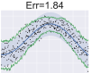
(b) GP

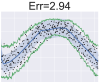
(c) NN

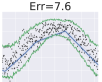
(d) BNN

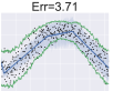
(e) MC-Dropout

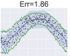
(f) Ens-NN

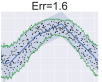
(g) Combined

Figure 2: Weather data with uncertainties. Dots are datapoints, green lines are the true uncertainty, blue curves are mean predictions and the blue shaded areas are the estimated uncertainties.

Ablation study.

To determine the influence of each methodology from Sec. 3, we experimented with four UCI regression datasets (Fig. 3). We split our contributions in four: the locality sampler (LS), the mean-variance split (MV), the inverse-gamma prior (IG) and the extrapolating architecture (EX). The combined model includes all four tricks. The results clearly shows that LS and IG methodologies has the most impact on test set log likelihood, but none of the methodologies perform worse than the baseline model. Combined they further improves the results, indicating that the proposed methodologies are complementary.

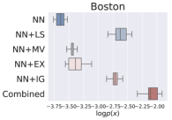
(a)

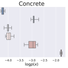
(b)

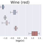
(c)

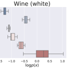
(d)

Figure 3: The complementary methodologies from Sec. 3 evaluated on UCI benchmark datasets.

UCI benchmark.

We now follow the experimental setup from Hernández-Lobato and Adams (2015), by evaluating models on a number of regression datasets from the UCI machine learning database. Additional to the standard benchmark, we have added 4 datasets. Test set log-likelihood can be seen in Table 1, and the corresponding RMSE scores can be found in the supplementary material.

	$N$	$D$	GP	SGP	NN	BNN	MC-Dropout	Ens-NN	Combined
Boston	506	13	$\mathbf{-1.76\pm 0.3}$	$-1.85\pm 0.25$	$-3.64\pm 0.09$	$-2.59\pm 0.11$	$-2.51\pm 0.31$	$-2.45\pm 0.25$	$-2.09\pm 0.09$
Carbon	10721	7	-	$3.74\pm 0.53$	$-2.03\pm 0.14$	$-1.1\pm 1.76$	$-1.08\pm 0.05$	$-0.44\pm 7.28$	$\mathbf{4.35\pm 0.16}$
Concrete	1030	8	$-2.13\pm 0.14$	$-2.29\pm 0.12$	$-4.23\pm 0.07$	$-3.31\pm 0.05$	$-3.11\pm 0.12$	$-3.06\pm 0.32$	$\mathbf{-1.78\pm 0.04}$
Energy	768	8	$-1.85\pm 0.34$	$-2.22\pm 0.15$	$-3.78\pm 0.04$	$-2.07\pm 0.08$	$-2.01\pm 0.11$	$\mathbf{-1.48\pm 0.31}$	$-1.68\pm 0.13$
Kin8nm	8192	8	-	$2.01\pm 0.02$	$-0.08\pm 0.02$	$0.95\pm 0.08$	$0.95\pm 0.15$	$1.18\pm 0.03$	$\mathbf{2.49\pm 0.07}$
Naval	11934	16	-	-	$3.47\pm 0.21$	$3.71\pm 0.05$	$3.80\pm 0.09$	$5.55\pm 0.05$	$\mathbf{7.27\pm 0.13}$
Power plant	9568	4	-	$-1.9\pm 0.03$	$-4.26\pm 0.14$	$-2.89\pm 0.01$	$-2.89\pm 0.14$	$-2.77\pm 0.04$	$\mathbf{-1.19\pm 0.03}$
Protein	45730	9	-	-	$-2.95\pm 0.09$	$-2.91\pm 0.00$	$-2.93\pm 0.14$	$\mathbf{-2.80\pm 0.02}$	$\mathbf{-2.83\pm 0.05}$
Superconduct	21263	81	-	$-4.07\pm 0.01$	$-4.92\pm 0.10$	$-3.06\pm 0.14$	$-2.91\pm 0.19$	$-3.01\pm 0.05$	$\mathbf{-2.43\pm 0.05}$
Wine (red)	1599	11	$0.96\pm 0.18$	$-0.08\pm 0.01$	$-1.19\pm 0.11$	$-0.98\pm 0.01$	$-0.94\pm 0.01$	$-0.93\pm 0.09$	$\mathbf{1.21\pm 0.23}$
Wine (white)	4898	11	-	$-0.14\pm 0.05$	$-1.29\pm 0.09$	$-1.41\pm 0.17$	$-1.26\pm 0.01$	$-0.99\pm 0.06$	$\mathbf{0.40\pm 0.42}$
Yacht	308	7	$\mathbf{0.16\pm 1.22}$	$-0.38\pm 0.32$	$-4.12\pm 0.17$	$-1.65\pm 0.05$	$-1.55\pm 0.12$	$-1.18\pm 0.21$	$\mathbf{-0.07\pm 0.05}$
Year	515345	90	-	-	$-5.21\pm 0.87$	$-3.97\pm 0.34$	$-3.78\pm 0.01$	$-3.42\pm 0.02$	$\mathbf{-3.01\pm 0.14}$

Table 1: Dataset characteristics and tests set log-likelihoods for the different methods. A - indicates the model was infeasible to train. Bold highlights the best results.

Our Combined model performs best on 10 of the 13 datasets. For the small Boston and Yacht datasets, the standard GP performs the best, which is in line with the experience that GPs perform well when data is scarce. On these datasets our model is the best-performing neural network. On the Energy and Protein datasets Ens-NN perform the best, closely followed by our Combined model. One clear advantage of our model compared to Ens-NN is that we only need to train one model, whereas Ens-NN need to train 5+ (see the supplementary material for training times for each model). The worst performing model in all cases is the baseline NN model, which clearly indicates that the usual tools for mean estimation does not carry over to variance estimation.

Active learning.

The performance of active learning depends on predictive uncertainty (Settles, 2009), so we use this to demonstrate the improvements induced by our method. We use the same network architectures and datasets as in the UCI benchmark. Each dataset is split into: 20% train, 60% pool and 20% test. For each active learning iteration, we first train a model, evaluate the performance on the test set and then estimate uncertainty for all datapoints in the pool. We then select the $n$ points with highest variance (corresponding to highest entropy (Houlsby et al., 2012)) and add these to the training set. We set $n=1\%$ of the initial pool size. This is repeated 10 times, such that the last model is trained on 30%. We repeat this on 10 random training-test splits to compute standard errors.

Fig. 4,show the evolution of average RMSE for each method during the data collection process for the Boston, Superconduct and Wine (white) datasets (all remaining UCI datasets are visualized in the supplementary material). In general, we observe two trends. For some datasets we observe that our Combined model outperforms all other models, achieving significantly faster learning. This indicates that our model is better at predicting the uncertainty of the data in the pool set. On datasets where the sampling process does not increase performance, we are on par with other models.

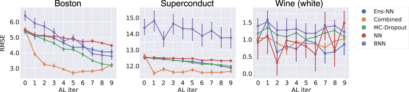
Figure 4: Average test set RMSE and standard errors in active learning. The remaining datasets are shown in the supplementary material.

4.2 Generative models

To show a broader application of our approach, we also explore it in the context of generative modeling. We focus on variational autoencoders (VAEs) (Kingma and Welling, 2013; Rezende et al., 2014) that are popular deep generative models. A VAE model the generative process:

$$p({\boldsymbol{x}})\!=\!\int p_{\theta}({\boldsymbol{x}}|{\boldsymbol{z}})p({\boldsymbol{z}})\mathrm{d}{\boldsymbol{z}},\quad p_{\theta}({\boldsymbol{x}}|{\boldsymbol{z}})\!=\!\mathcal{N}\big{(}{\boldsymbol{x}}|\mu_{\theta}({\boldsymbol{z}}),\sigma_{\theta}^{2}({\boldsymbol{z}})\big{)}\text{\quad or\quad}p_{\theta}({\boldsymbol{x}}|{\boldsymbol{z}})\!=\!\mathcal{B}\big{(}{\boldsymbol{x}}|\mu_{\theta}({\boldsymbol{z}})\big{)},$$ (6)

where $p({\boldsymbol{z}})=\mathcal{N}(\textbf{0},\mathbb{I}_{d})$. This is trained by introducing a variational approximation $q_{\phi}({\boldsymbol{z}}|{\boldsymbol{x}})=\mathcal{N}({\boldsymbol{z}}|\mu_{\phi}({\boldsymbol{x}}),\sigma_{\phi}^{2}({\boldsymbol{x}}))$ and then jointly training $p_{\theta}$ and $q_{\phi}$. For our purposes, it suffcient to note that a VAE estimates both a mean and a variance function. Thus using standard training methods, the same problems arise as in the regression setting. Mattei and Frellsen (2018) have recently shown that estimating a VAE is ill-posed unless the variance is bounded from below. In the literature, we often find that

1. Variance networks are avoided by using a Bernoulli distribution, even if data is not binary.

2. Optimizing VAEs with a Gaussian posterior is considerably harder than the Bernoulli case. To overcome this, the variance is often set to a constant e.g. $\sigma^{2}({\boldsymbol{z}})=1$. The consequence is that the log-likelihood reconstruction term in the ELBO collapses into an L2 reconstruction term.

3. Even though the generative process is given by Eq. 6, samples shown in the literature are often reduced to $\tilde{{\boldsymbol{x}}}=\mu({\boldsymbol{z}}),{\boldsymbol{z}}\sim\mathcal{N}(\textbf{0},\mathbb{I})$. This is probably due to the wrong/meaningless variance term.

We aim to fix this by training the posterior variance $\sigma_{\theta}^{2}({\boldsymbol{z}})$ with our Combined method. We do not change the encoder variance $\sigma_{\phi}^{2}({\boldsymbol{x}})$ and leave this to future study.

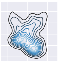
(a)

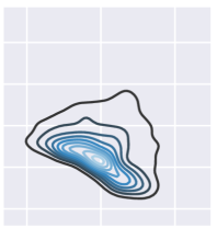
(b)

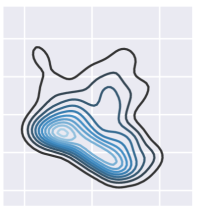
(c)

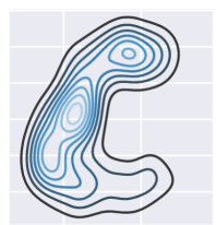
(d) Ground truth

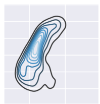
(e) VAE

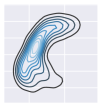
(f) Comb-VAE

Figure 5: The ground truth and generated distributions.
Top: $x_{1}$ vs. $x_{2}$. Bottom: $x_{2}$ vs $x_{3}$.

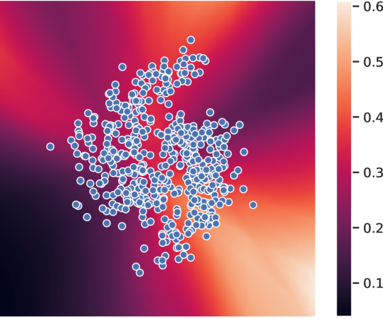
(a)

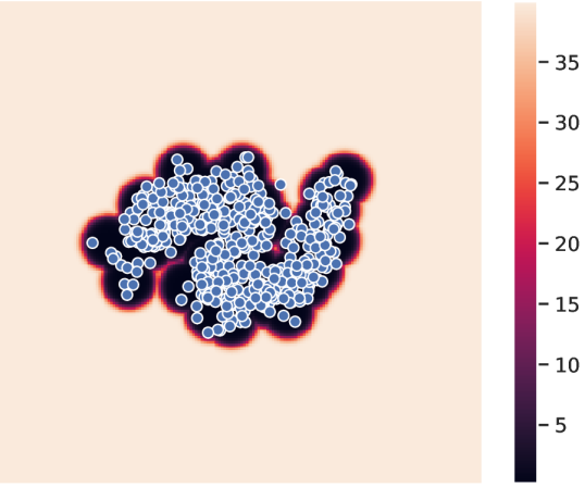
(b)

figureVariance estimates in latent space for standard VAE (top) and our Comb-VAE (bottom). Blue points are the encoded training data.

Artificial data.

We first evaluate the benefits of more reliable variance networks in VAEs on artificial data. We generate data inspired by the two moon dataset, which we map into four dimensions. The mapping is thoroughly described in the supplementary material, and we emphasize that we have deliberately used mappings that MLP’s struggle to learn, thus with a low capacity network the only way to compensate is to learn a meaningful variance function.

In Fig. 5 we plot pairs of output dimensions using 5000 generated samples. For all pairwise combinations we refer to the supplementary material. We observe that samples from our Comb-VAE capture the data distribution in more detail than a standard VAE. For VAE the variance seems to be underestimated, which is similar to the results from regression. The poor sample quality of a standard VAE can partially be explained by the arbitrariness of decoder variance function $\sigma^{2}({\boldsymbol{z}})$ away from data. In Fig. 6b, we calculated the accumulated variance $\sum_{j=1}^{D}\sigma^{2}_{j}({\boldsymbol{z}})$ over a grid of latent points. We clearly see that for the standard VAE, the variance is low where we have data and arbitrary away from data. However, our method produces low-variance region where the two half moons are and a high variance region away from data. We note that Arvanitidis et al. (2018) also dealt with the problem of arbitrariness of the decoder variance. However their method relies on post-fitting of the variance, whereas ours is fitted during training. Additionally, we note that (Takahashi et al., 2018) also successfully modeled the posterior of a VAE as a Student t-distribution similar to our proposed method, but without the extrapolation and different training procedure.

		MNIST	FashionMNIST	CIFAR10	SVHN
ELBO	VAE	2053.01 $\pm$ 1.60	1506.31 $\pm$ 2.71	1980.84 $\pm$ 3.32	3696.35 $\pm$ 2.94
	Comb-VAE	2152.31 $\pm$ 3.32	1621.29 $\pm$ 7.23	2057.32 $\pm$ 8.13	3701.41 $\pm$ 5.84
$\log p(x)$	VAE	1914.77 $\pm$ 2.15	1481.38 $\pm$ 3.68	1809.43 $\pm$ 10.32	3606.28 $\pm$ 2.75
	Comb-VAE	2018.37 $\pm$ 4.35	1567.23 $\pm$ 4.82	1891.39 $\pm$ 20.21	3614.39 $\pm$ 7.91

Table 2: Generative modeling of 4 datasets. For each dataset we report training ELBO and test set log-likelihood. The standard errors are calculated over 3 trained models with random initialization.

Image data.

For our last set of experiments we fitted a standard VAE and our Comb-VAE to four datasets: MNIST, FashionMNIST, CIFAR10, SVHN. We want to measure whether there is an improvement to generative modeling by getting better variance estimation. The details about network architecture and training can be found in the supplementary material. Training set ELBO and test set log-likelihoods can be viewed in Table 2. We observe on all datasets that, on average tighter bounds and higher log-likelihood are achieved, indicating that we better fit the data distribution. We quantitatively observe (see Fig. 6) that variance has a more local structure for Comb-VAE and that the variance reflects the underlying latent structure.

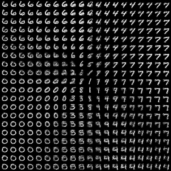
(c)

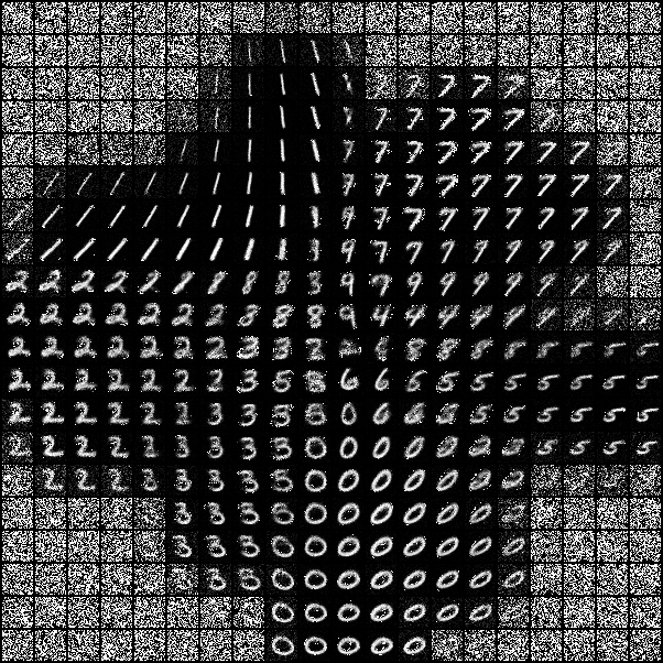
(d)

Figure 6: Generated MNIST images on a grid in latent space using the standard variance network (left) and proposed variance network (right).

5 Discussion & Conclusion

While variance networks are commonly used for modeling the predictive uncertainty in regression and in generative modeling, there have been no systematic studies of how to fit these to data. We have demonstrated that tools developed for fitting mean networks to data are subpar when applied to variance estimation. The key underlying issue appears to be that it is not feasible to estimate both a mean and a variance at the same time, when data is scarce.

While it is beneficial to have separate estimates of both epistemic and aleatoric uncertainty, we have focused on predictive uncertainty, which combine the two. This is a lesser but more feasible goal.

We have proposed a new mini-batching scheme that samples locally to ensure that variances are better defined during model training. We have further argued that variance estimation is more meaningful when conditioned on the mean, which implies a change to the usual training procedure of joint mean-variance estimation. To cope with data scarcity we have proposed a more robust likelihood that model a distribution over the variance. Finally, we have highlighted that variance networks need to extrapolate differently from mean networks, which implies architectural differences between such networks. We specifically propose a new architecture for variance networks that ensures similar variance extrapolations to posterior Gaussian processes from stationary priors.

Our methodologies depend on algorithms that computes Euclidean distances. Since these often break down in high dimensions, this indicates that our proposed methods may not be suitable for high dimensional data. Since we mostly rely on nearest neighbor computations, that empirical are known to perform better in high dimensions, our methodologies may still work in this case. Interestingly, the very definition of variance is dependent on Euclidean distance and this may indicate that variance is inherently difficult to estimate for high dimensional data. This could possible be circumvented through a learned metric.

Experimentally, we have demonstrated that proposed methods are complementary and provide significant improvements over state-of-the-art. In particular, on benchmark data we have shown that our method improves upon the test set log-likelihood without improving the RMSE, which demonstrate that the uncertainty is a significant improvement over current methods. Another indicator of improved uncertainty estimation is that our method speeds up active learning tasks compared to state-of-the-art. Due to the similarities between active learning, Bayesian optimization, and reinforcement learning, we expect that our approach carries significant value to these fields as well. Furthermore, we have demonstrated that variational autoencoders can be improved through better generative variance estimation. Finally, we note that our approach is directly applicable alongside ensemble methods, which may further improve results.

Acknowledgements.

This project has received funding from the European Research Council (ERC) under the European Union’s Horizon 2020 research and innovation programme (grant agreement n^o 757360). NSD, MJ and SH were supported in part by a research grant (15334) from VILLUM FONDEN. We gratefully acknowledge the support of NVIDIA Corporation with the donation of GPU hardware used for this research.

Appendix A Further results

Gradient experiments

In Fig. 7 we have plotted the sparsity index and variance of gradient for both the mean (top row) and variance function (bottom row). We do this for both normal mini-batching and our proposed locality sampler. Sparsity is measured as $\ell_{0.001}^{0}(\nabla)=\{j,\nabla_{j}\leq 0.001\}$ and the sparsity index is then given by $\text{SI}=\frac{\ell_{0.001}^{0}(\nabla)}{|\nabla|}$. We observe for the mean function, that the sparsity index and variance is similar for the two methods, indicating that our locality sampler does not improve on the fitting of the mean function, as expected. However for the variance function we see a clear gap in sparsity and variance, indicating that our locality sampler gives more local and stable updates to variance networks.

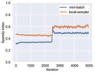
(a)

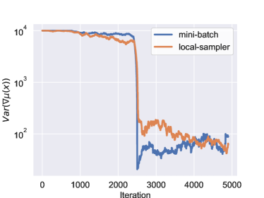
(b)

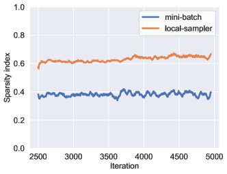
(c)

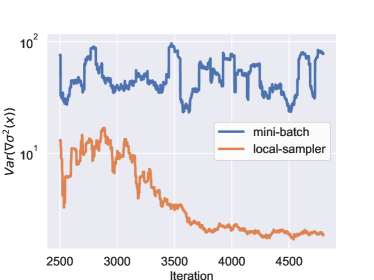
(d)

Figure 7: Left: Sparsity index for mean (top) and variance (bottom) network. Right: Variance of gradient for mean (top) and variance (bottom) network. The variance network was disabled for the first 2500 iterations, to warm up the mean function to secure convergence.

UCI benchmark (RMSE)

In Table 3 the test set RMSE results for the UCI regression benchmark can be seen. We clearly observe that all neural network based methods achieve nearly identical RMSE for all datasets, indicating that the mean function is similarly trained for all the methods.

	$N$	$D$	GP	SGP	NN	BNN	MC-Dropout	Ens-NN	Combined
Boston	506	13	2.79 $\pm$ 0.52	2.98 $\pm$ 0.55	4.45 $\pm$ 1.41	3.45 $\pm$ 0.87	3.01 $\pm$ 0.99	3.33 $\pm$ 1.33	3.11 $\pm$ 0.35
Carbon	10721	7	-	1.01 $\pm$ 0.01	0.41 $\pm$ 0.0	0.18 $\pm$ 0.1	0.29 $\pm$ 0.0	0.41 $\pm$ 0.0	0.35 $\pm$ 0.01
Concrete	1030	8	6.03 $\pm$ 0.59	6.45 $\pm$ 0.64	7.71 $\pm$ 1.32	5.78 $\pm$ 0.21	5.33 $\pm$ 0.65	5.65 $\pm$ 0.55	5.75 $\pm$ 0.41
Energy	768	8	1.98 $\pm$ 0.76	2.12 $\pm$ 0.56	1.67 $\pm$ 0.44	1.89 $\pm$ 0.04	1.69 $\pm$ 0.19	2.13 $\pm$ 0.46	1.70 $\pm$ 0.21
Kin8nm	8192	8	-	0.08 $\pm$ 0.0	0.21 $\pm$ 0.01	0.18 $\pm$ 0.02	0.12 $\pm$ 0.01	0.01 $\pm$ 0.01	0.12 $\pm$ 0.01
Naval	11934	16	-	-	0.01 $\pm$ 0.0	0.01 $\pm$ 0.0	0.01 $\pm$ 0.0	0.01 $\pm$ 0.0	0.01 $\pm$ 0.0
Power plant	9568	4	-	4.65 $\pm$ 0.12	4.23 $\pm$ 0.33	4.12 $\pm$ 0.45	4.13 $\pm$ 0.13	4.11 $\pm$ 0.21	4.12 $\pm$ 0.13
Protein	45730	9	-	-	4.38 $\pm$ 0.07	4.67 $\pm$ 0.94	4.19 $\pm$ 0.08	4.36 $\pm$ 0.07	4.52 $\pm$ 0.19
Superconduct	21263	81	-	11.32 $\pm$ 0.38	11.73 $\pm$ 0.46	11.07 $\pm$ 1.7	11.44 $\pm$ 0.39	11.63 $\pm$ 0.49	11.65 $\pm$ 0.65
Wine (red)	1599	11	0.88 $\pm$ 0.06	0.65 $\pm$ 0.04	0.66 $\pm$ 0.06	0.69 $\pm$ 0.41	0.64 $\pm$ 0.06	0.67 $\pm$ 0.06	0.68 $\pm$ 0.11
Wine (white)	4898	11	-	0.65 $\pm$ 0.03	0.67 $\pm$ 0.04	0.68 $\pm$ 0.32	0.71 $\pm$ 0.04	0.78 $\pm$ 0.04	0.72 $\pm$ 0.09
Yacht	308	7	0.42 $\pm$ 0.21	0.72 $\pm$ 0.21	1.63 $\pm$ 0.61	1.05 $\pm$ 0.11	1.11 $\pm$ 0.48	1.58 $\pm$ 0.58	1.27 $\pm$ 0.11
Year	515345	90	-	-	12.47 $\pm$ 0.96	9.01 $\pm$ 0.45	8.92 $\pm$ 0.23	8.88 $\pm$ 0.13	8.85 $\pm$ 0.05

Table 3: Dataset characteristics and RMSE for the different methods. A - indicates the models was infeasible to train.

Timings of models

In Table 4 we show the average computation time for each model. The experiments was conducted with an Intel Xeon E5-2620v4 CPU and Nvidia GTX TITAN X GPU. We note that our model suffers from long computations for very large datasets, mainly due to the computation of the neighborhood graph in the locality sampler. This could be reduced by using fast approximative method for k-nearest-neighbor and by reducing data dimensionality e.g. PCA dimensionality reduction.

	$N$	$D$	GP	SGP	NN	BNN	MC-Dropout	Ens-NN	Combined
Boston	506	13	8.37 +- 2.92	91.86 +- 30.12	94.04 +- 2.24	81.32 +- 1.83	98.08 +- 2.0	479.1 +- 12.49	93.39 +- 1.82
Carbon	10721	7	-	192.57 +- 72.28	90.05 +- 3.4	80.95 +- 2.04	98.62 +- 1.85	439.45 +- 23.01	123.61 +- 2.84
Concrete	1030	8	7.48 +- 1.2	173.73 +- 4.0	92.91 +- 4.17	81.02 +- 2.04	97.94 +- 1.84	468.94 +- 10.81	97.65 +- 6.4
Energy	768	8	10.48 +- 4.12	121.39 +- 52.2	92.91 +- 2.14	80.92 +- 2.14	97.86 +- 2.13	475.04 +- 12.61	93.01 +- 1.29
Kin8nm	8192	8	-	1526.29 +- 20.28	92.22 +- 4.65	80.65 +- 2.11	97.85 +- 2.87	459.81 +- 27.66	123.15 +- 2.86
Navel	11934	16	-	9.79 +- 0.23	91.2 +- 3.28	82.97 +- 1.84	98.64 +- 1.89	482.74 +- 8.54	136.25 +- 3.29
Power	9568	4	-	1267.82 +- 783.28	92.23 +- 3.28	81.29 +- 1.98	98.26 +- 1.87	472.39 +- 9.73	118.26 +- 1.86
Protein	45730	9	-	-	138.49 +- 2.51	124.72 +- 1.86	140.73 +- 3.32	707.69 +- 11.02	658.63 +- 11.75
Superconduct	21263	81	-	313.9 +- 2.9	95.27 +- 3.43	90.71 +- 1.86	90.25 +- 1.67	477.57 +- 11.91	235.72 +- 3.8
Wine (red)	1599	11	35.33 +- 19.09	262.69 +- 10.14	93.51 +- 2.09	80.67 +- 2.04	97.78 +- 2.58	416.02 +- 23.9	130.61 +- 7.91
Wine (white)	4898	11	-	781.13 +- 8.2	91.97 +- 2.41	80.94 +- 1.75	97.61 +- 2.73	451.65 +- 19.04	99.44 +- 1.33
Yacht	308	7	0.93 +- 0.32	22.74 +- 11.98	92.82 +- 3.47	81.0 +- 1.92	98.27 +- 1.68	422.9 +- 35.85	105.33 +- 2.32
Year	515345	90	-	-	139.45 +- 6.15	643.96 +- 4.17	77.96 +- 2.09	725.27 +- 20.08	2453.62 +- 18.7

Table 4: Timings(s) for the different models evaluated on the UCI benchmark

Ablation study (RMSE)

In Fig. 8 we have plotted the RMSE for different combinations of our methodologies. Since the RMSE is only influenced by how well $\mu(x)$ is fitted, the difference in log likelihood that we observe between the models (see paper) must be explained by how well $\sigma^{2}(x)$ is fitted.

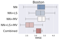
(a)

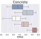
(b)

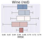
(c)

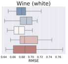
(d)

Figure 8: Our contributions evaluated on four different UCI benchmark datasets.

Active learning

In Figs. 9m and 10m we respective shows the progress of RMSE and log likelihood on all 13 dataset. We observe that for some of the datasets (Boston, Superconduct, Power) our proposed Combine model achieves faster learning than other methods. On all other datasets we are equally good as the best performing model.

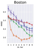
(a)

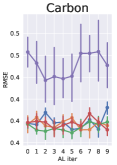
(b)

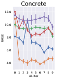
(c)

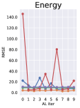
(d)

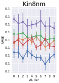
(e)

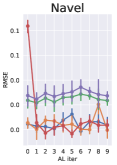
(f)

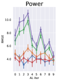
(g)

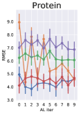
(h)

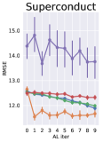
(i)

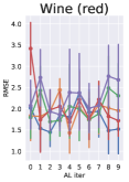
(j)

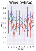
(k)

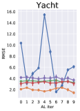
(l)

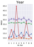
(m)

Figure 9: Average test RMSE and standard errors in the active learning experiments for all datasets.

(n)

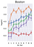
(a)

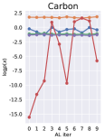
(b)

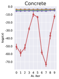
(c)

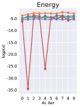
(d)

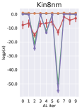
(e)

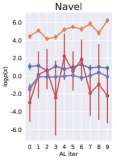
(f)

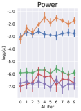
(g)

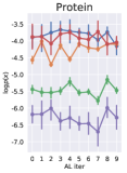
(h)

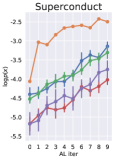
(i)

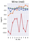
(j)

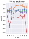
(k)

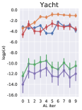
(l)

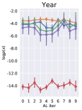
(m)

Figure 10: Average test log likelihood and standard errors in the active learning experiments for all datasets.

(n)

Generative modeling toy data

In Fig. 12 we show marginal distribution, pairwise pointplots and pairwise joint distribution for our artificially dataset used in the generative setting. Top row show the ground true data, middle row shows reconstructions and samples from standard VAE model and bottom row show reconstructions and samples from our proposed Comb-VAE model. We observe that reconstruction are similar for the two models, but the quality of the generative samples are much better for Comb-VAE.

Generative modeling of image data

In Fig. 11 we show a meshgrid of samples from VAE and Comb-VAE on the MNIST dataset. We clearly see how proper extrapolation of variance in Comb-VAE can be used to "mask" when we are inside our data region and when we are outside. For standard VAE we observe a near constant variance added to the images.

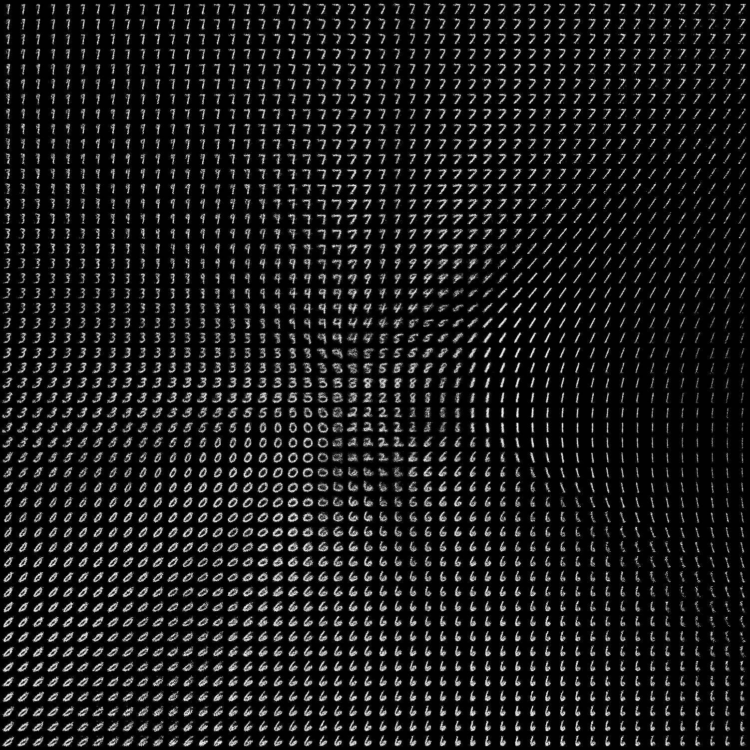
(a) VAE

(b) Comb-VAE

Figure 11: Meshgrid of latent space. For each subplot we sampled a mesh grid $[-4,4]\times[-4,4]$ of $[50,50]$ points, which we used to generate samples from.

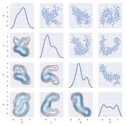
(a) Ground true

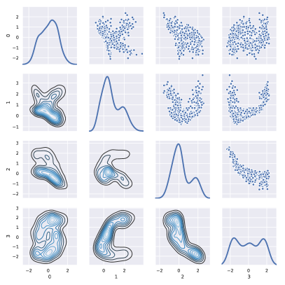
(b) VAE (R)

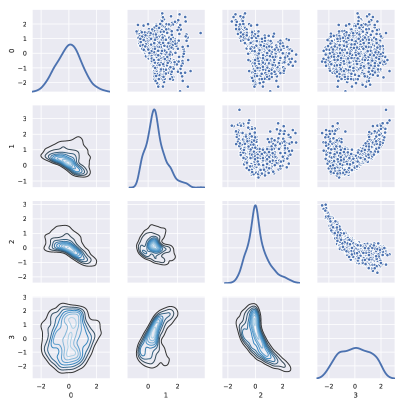
(c) VAE (S)

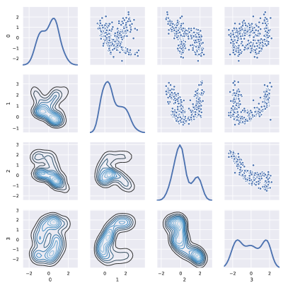
(d) Comb-VAE (R)

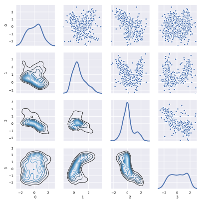
(e) Comb-VAE (S)

Figure 12: Pairwise plots between all sets of variables for our artificially dataset in the generative setting.

Appendix B On the parametrization of the $t$-distributed predictive distribution

We parametrize the Student-$t$ distribution by letting the variance $\sigma^{2}$ have an inverse-Gamma distribution with shape and scale parameters $\alpha$ and $\beta$. We use that if $\sigma^{2}\sim\textsc{Inv-Gamma}(\alpha,\beta)$ then $\frac{1}{\sigma^{2}}\sim\Gamma(\alpha,\beta)$. Then

$$p(y|\mu,\alpha,\beta) =\int_{0}^{\infty}\mathcal{N}(y|\mu,\sigma^{2})\frac{\beta^{\alpha}}{\Gamma(\alpha)}(\sigma^{2})^{-(\alpha+1)}\exp(-\frac{\beta}{\sigma^{2}})\text{d}\sigma^{2}$$

$$=\frac{\beta^{\alpha}}{\Gamma(\alpha)\sqrt{2\pi}}\int_{0}^{\infty}(\sigma^{2})^{-(\alpha+1)-\frac{1}{2}}\exp(-\frac{1}{\sigma^{2}}(\beta+\frac{1}{2}(y-\mu)^{2}))\text{d}\sigma^{2}$$

$$=\frac{\beta^{\alpha}}{\Gamma(\alpha)\sqrt{2\pi}}\frac{\Gamma(\alpha+\frac{1}{2})}{\Big{(}\beta+\frac{1}{2}(y-\mu)^{2}\Big{)}^{\alpha+\frac{1}{2}}},$$

where we substituted the variable $\sigma^{2}$ with $\frac{1}{\sigma^{2}}$ and used that the remaining was a Gamma integral.

Appendix C Parameters of the locality sampler

In Algorithm 1 a pseudoimplementation of our proposed locality sampler can be seen. The two important parameters in this algorithm are the primary sampling units (psu) and secondary sampling units (ssu). In Fig. 13 and 14 we visually show the effect of these two parameters.

For all our experiments we set psu=3 and ssu=40 when we are training the mean function and for variance function we set psu=1 and ssu=10.

Algorithm 1 Locality-sampler

Input $N$ datapoints, a metric $d$ on feature space $\mathbb{R^{D}}$, integers $m,n,k$.

1:For each datapoint calculate the $k$ nearest neighbors under the metric $d$.

2:Sample $m$ primary sampling units with uniform probability without replacement among all $N$ units.

3:For each of the primary sampling units sample $n$ secondary sampling units among the primary sampling units $k$ nearest neighbors with uniform probability without replacement.

Output All secondary sampling units is a sample of at most $m\cdot n$ points. If a new sample is needed repeat from Step 2.

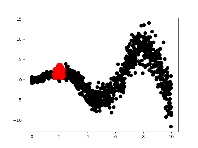
(a)

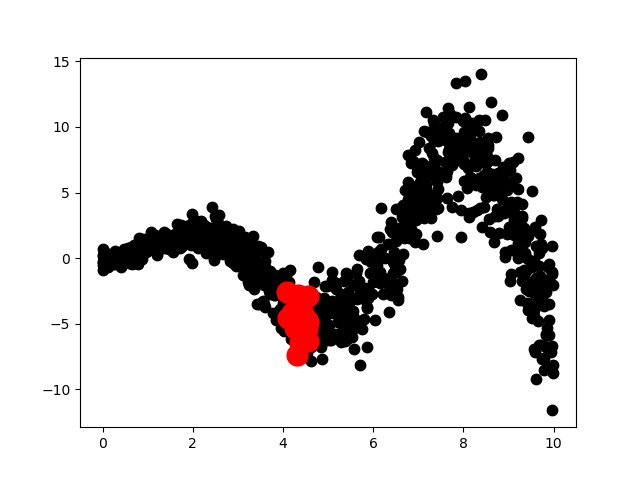
(b)

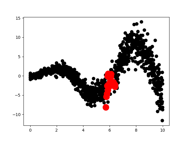
(c)

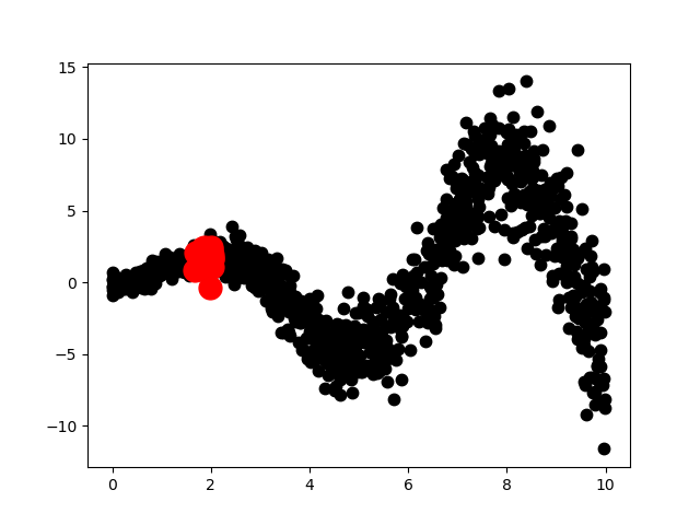
(d)

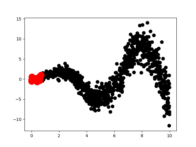
(e)

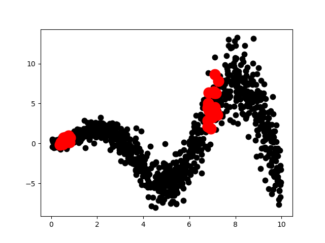
(f)

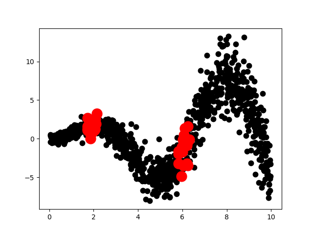
(g)

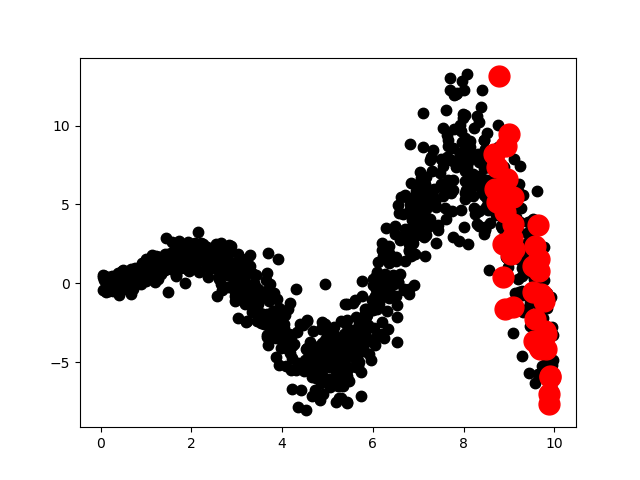
(h)

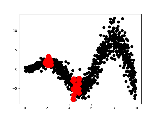
(i)

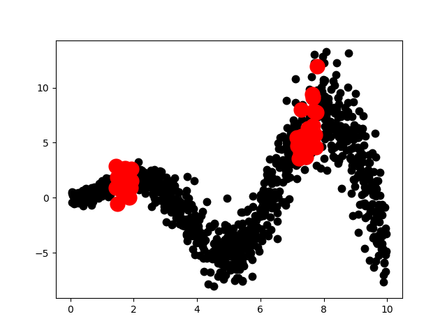
(j)

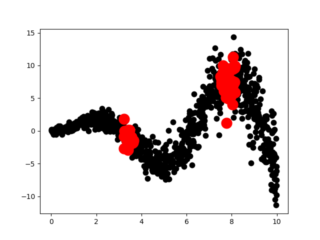
(k)

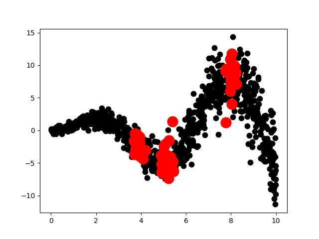
(l)

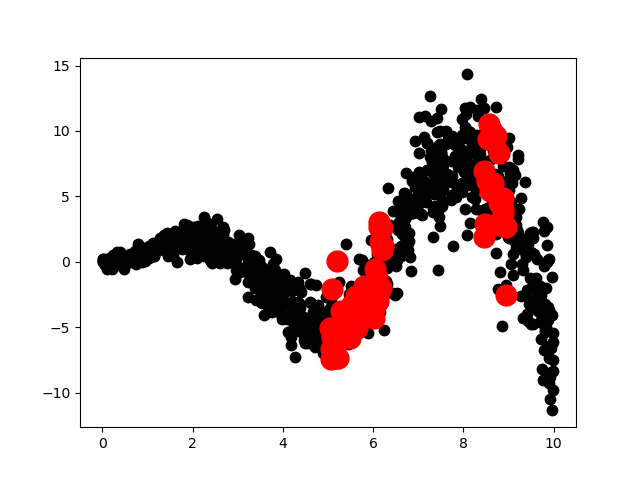
(m)

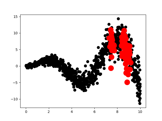
(n)

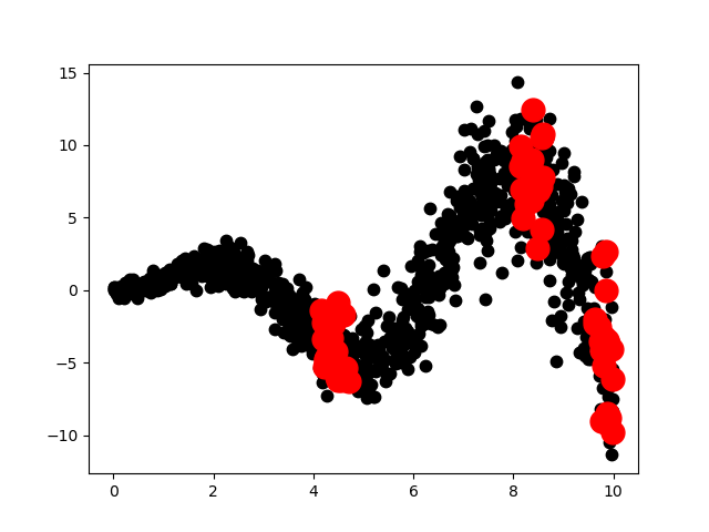
(o)

Figure 13: The effect of changing the size of the primary sampling unit. From top to bottom: $psu=[1,2,3]$. Each column corresponds to a sample from the locality sampler.

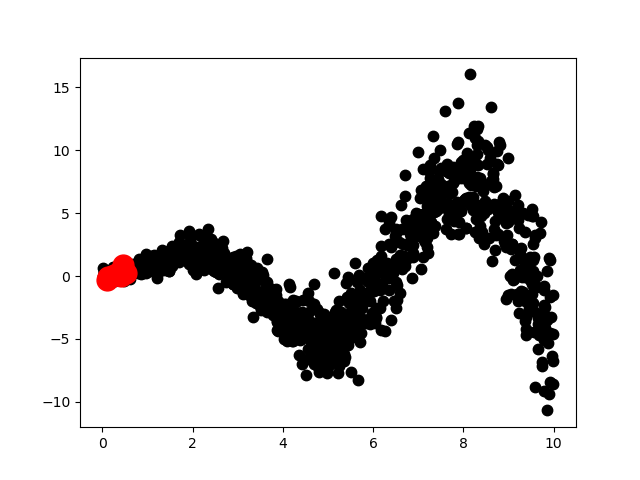
(a)

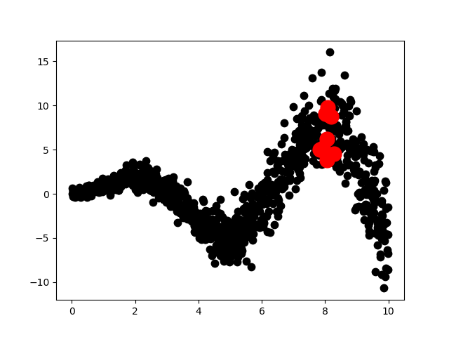
(b)

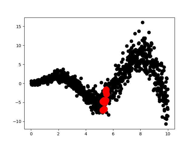
(c)

(d)

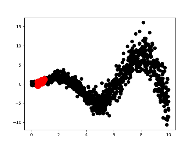
(e)

(f)

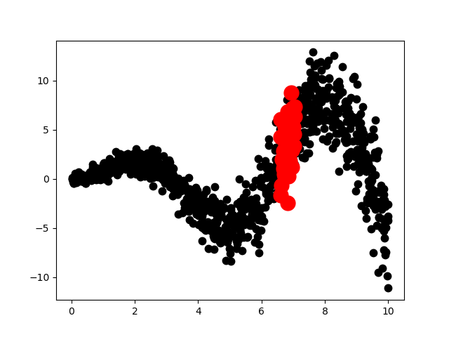
(g)

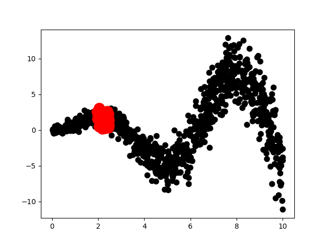
(h)

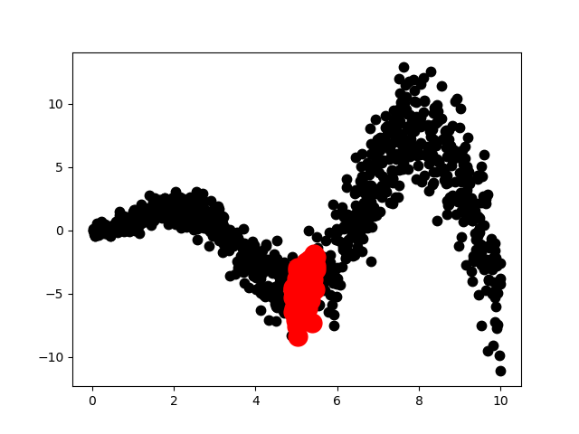
(i)

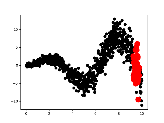
(j)

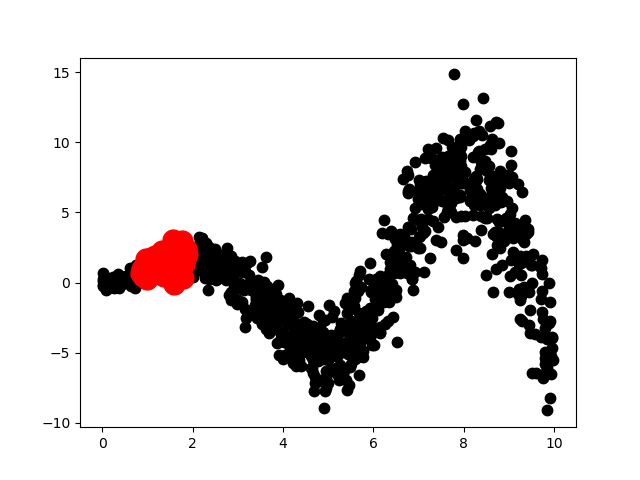
(k)

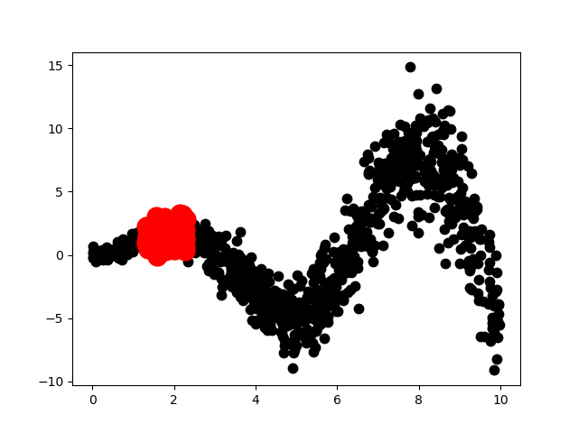
(l)

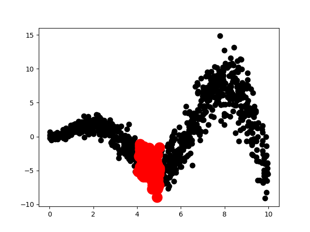
(m)

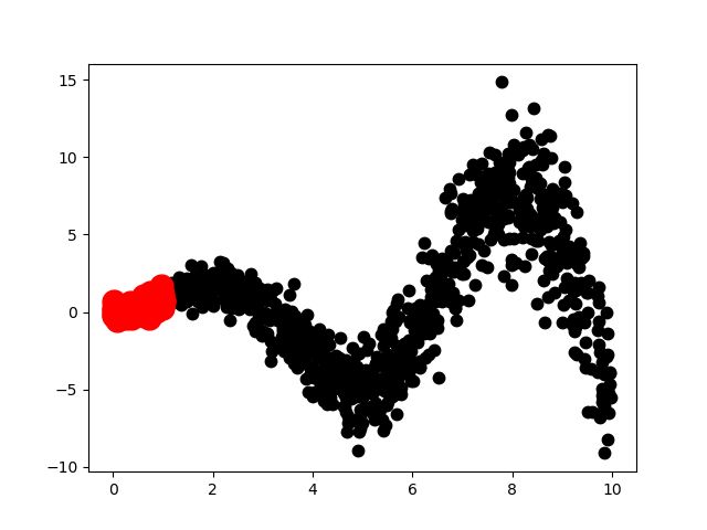
(n)

(o)

Figure 14: The effect of changing the size of the secondary sampling unit. From top to bottom: $ssu=[10,50,100]$. Each column corresponds to a sample from the locality sampler.

Appendix D Implementation details for regression experiments

All neural network based models were implemented in Pytorch (Paszke et al., 2017), except for the Baysian neural network which was implemented in Tensorflow (Abadi et al., 2015). GP models where implemented in GPy (GPy, since 2012). Below we have stated details for all models:

GP

Fitted using a ARD kernel and with default settings of GPy.

SGP

Fitted using a ARD kernel and with default settings of GPy. Number of inducing points was set to $\min(500,|\mathcal{D}_{train}|)$.

NN

Model use two networks, one for the predictive mean and one for the predictive variance. Model was trained to optimize the log-likelihood of data.

BNN

We use a standard factored Gaussian prior for the weights and use the Flipout approximation (wen2018flipout) for the variational approximation.

MC-Dropout

Model use a single network, where we place dropout on all weights. The dropout weight was set to 0.05. The model was trained to optimize the RMSE of data.

Ens-NN

Model consist of an ensemble of 5 individual NN models, each modeled as two individual networks. Each are trained to optimize the log-likelihood of data. Only difference between ensemble models is initialization.

Combined

Model use three networks, one for the mean function, one for the $\alpha$ parameter and one for the $\beta$ parameter. We set the number of inducing points to $\min(500,|\mathcal{D}_{train}|)$. For the $\gamma$ in the scaled-and-translated sigmoid function $\nu(x)$ we initialize it to 1.5, and try to minimize it during training. Model was trained to optimize the log-likelihood of data.

For each neural network based approach, we follow the experimental setup (Hernández-Lobato and Adams, 2015). All individual networks was modeled a single hidden layer MLPs with 50 neurons for all other datasets than "Protein" and "Year" where we use 100 neurons. Except for the output of each network, the activation function used is ReLU. For the output of the mean networks, no activation function is applied. For the output of the variance network, the Softplus activation function is used to secure positive variance. All neural network based models where trained using the Adam optimizer (Kingma and Ba, 2015) with a learning rate of $10^{-1}$ using a batch size of 256. All models were trained for 10.000 iterations.

The code can found here: https://github.com/SkafteNicki/john.

Appendix E Generative network architecture

Pixel values of the images were scaled to the interval [0,1]. Each pixel is assumed to be i.i.d. Gaussian distributed. For the encoders and decoders we use multilayer perceptron networks, see table below.

	Layer 1	Layer 2	Layer 3	Layer 4
$\bm{\mu}_{encoder}$	512 (BN + ReLU)	256 (BN + ReLU)	128 (BN + ReLU)	d (BN + Linear)
$\bm{\sigma}^{2}_{encoder}$	512 (BN + ReLU)	256 (BN + ReLU)	128 (BN + ReLU)	d (Softplus)
$\bm{\mu}_{decoder}$	128 (BN + ReLU)	256 (BN + ReLU)	512 (BN + ReLU)	D (ReLU)
$\bm{\sigma}^{2}_{decoder}$	128 (BN + ReLU)	256 (BN + ReLU)	512 (BN + ReLU)	D (Softplus)

The numbers corresponds to the size of the layer and the parenthesis states the used activation function and whether or not batch normalization was used. $D$ indicates the size of the images i.e. $D=width\times height\times channels$. For MNIST and FashionMNIST these are 28,28,1 and for CIFAR10 and SVHN these are 32,32,1. $d$ indicates the size of the latent space. For MNIST and FashionMNIST we set $d=2$ for visualization purpose and for CIFAR10 and SVHN we set $d=10$ to be able to capture the higher complexity of these datasets.

To train the networks we used the Adam optimizer (Kingma and Ba, 2015) with learning rate $10^{-3}$ and a batch size of 512. We train for 20000 iterations without early stopping. Additionally, we use warm-up for the KL term (Sønderby et al., 2016), by scaling it with $w=\text{min}\left(1,\frac{it}{warmup}\right)$ where $it$ is the current iteration number and $warmup$ was set to half the number of iterations. This secures that we converge to stable reconstructions before introducing too much structure in the latent space.

Appendix F Artificial Data

The data considered in Section 4 are generated in the following way: first we sample points in $\mathbb{R}^{2}$ in a two-moon type way. See details in Algorithm 2. We generate 500 points in this way to establish a ’known’ latent space. We then map these to four dimensions $(v_{1},v_{2},v_{3},v_{4})$ by

$$v_{1}(z_{1},z_{2}) =z_{1}-z_{2}+\epsilon\cdot\sqrt{0.03+0.05\cdot(3+z_{1})},$$ (7)

$$v_{2}(z_{1},z_{2}) =z_{1}^{2}+\frac{1}{2}z_{2}+\epsilon\cdot\sqrt{0.03+0.03\cdot\|\mathbf{z}\|_{2}},$$ (8)

$$v_{3}(z_{1},z_{2}) =z_{1}z_{2}-z_{1}+\epsilon\cdot\sqrt{0.03+0.05\cdot\|\mathbf{z}\|_{2}},$$ (9)

$$v_{4}(z_{1},z_{2}) =z_{1}+z_{2}+\epsilon\cdot\sqrt{0.03+\frac{0.03}{0.2+\|\mathbf{z}\|_{2}}},$$ (10)

where all $\epsilon\sim\mathcal{N}(0,1)$ and independent.

Algorithm 2 Two moon sampler

1:Sample $U\sim\text{Bernoulli}(0.5)$.

2:if $U=1$ then

3:     Set $c=(0.5,0)$ and sample $\alpha_{1}\sim\text{unif}[0,\pi]$.

4:     Let $z=c+(\cos(\alpha_{1}),\sin(\alpha_{1}))$, and sample $\alpha_{2}\sim\text{unif}[0,2\pi]$ and $u\sim\text{unif}[0,1]$.

5:     Let $z=z+\frac{u}{4}\cdot(\cos(\alpha_{2}),\sin(\alpha_{2}))$.

6:else

7:     Set $c=(-0.5,0)$ and sample $\alpha_{1}\sim\text{unif}[\pi,2\pi]$.

8:     Let $z=c+(\cos(\alpha_{1}),\sin(\alpha_{1}))$, and sample $\alpha_{2}\sim\text{unif}[0,2\pi]$ and $u\sim\text{unif}[0,1]$.

9:     Let $z=z+\frac{u}{4}\cdot(\cos(\alpha_{2}),\sin(\alpha_{2}))$. return $z$

A typical dataset from this procedure is shown in Figure 15.

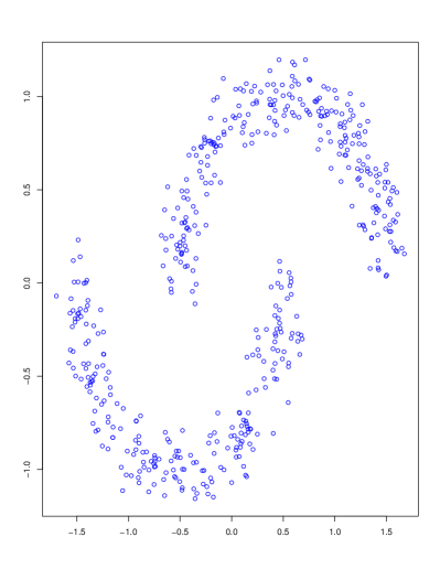
(a)

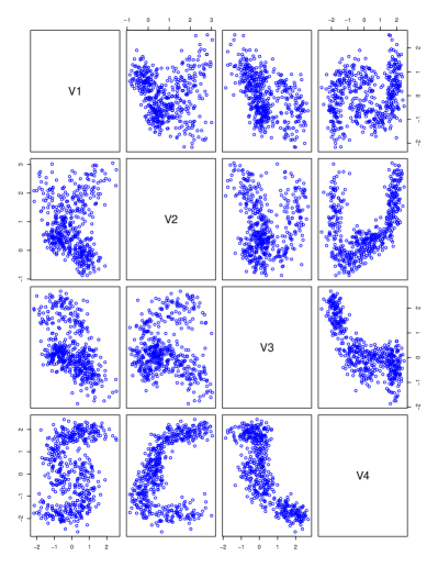
(b)

Figure 15: An example of the two moon data, and its transformation into $\mathbb{R}^{4}$. Shown as pairwise scatterplots.

References

- Abadi et al. [2015] M. Abadi, A. Agarwal, P. Barham, E. Brevdo, Z. Chen, C. Citro, G. S. Corrado, A. Davis, J. Dean, M. Devin, S. Ghemawat, I. Goodfellow, A. Harp, G. Irving, M. Isard, Y. Jia, R. Jozefowicz, L. Kaiser, M. Kudlur, J. Levenberg, D. Mané, R. Monga, S. Moore, D. Murray, C. Olah, M. Schuster, J. Shlens, B. Steiner, I. Sutskever, K. Talwar, P. Tucker, V. Vanhoucke, V. Vasudevan, F. Viégas, O. Vinyals, P. Warden, M. Wattenberg, M. Wicke, Y. Yu, and X. Zheng. TensorFlow: Large-scale machine learning on heterogeneous systems, 2015. URL https://www.tensorflow.org/. Software available from tensorflow.org.
- Amodei et al. [2016] D. Amodei, C. Olah, J. Steinhardt, P. Christiano, J. Schulman, and D. Mané. Concrete problems in ai safety. arXiv preprint arXiv:1606.06565, 2016.
- Arvanitidis et al. [2018] G. Arvanitidis, L. K. Hansen, and S. Hauberg. Latent space oddity: on the curvature of deep generative models. In International Conference on Learning Representations, 2018.
- Bishop [1994] C. M. Bishop. Mixture density networks. Technical report, Citeseer, 1994.
- Damianou and Lawrence [2013] A. Damianou and N. D. Lawrence. Deep gaussian processes. Proceedings of the 16th International Conference on Artificial Intelligence and Statistics (AISTATS), 2013.
- Frazier [2018] P. I. Frazier. A tutorial on bayesian optimization. arXiv preprint arXiv:1807.02811, 2018.
- Fu and Cai [2016] C. Fu and D. Cai. Efanna : An extremely fast approximate nearest neighbor search algorithm based on knn graph. 09 2016.
- Gal and Ghahramani [2016] Y. Gal and Z. Ghahramani. Dropout as a bayesian approximation: Representing model uncertainty in deep learning. In international Conference on Machine Learning, pages 1050–1059, 2016.
- Gelman et al. [2014] A. Gelman, J. B. Carlin, H. S. Stern, D. B. Dunson, A. Vehtari, and D. B. Rubin. Bayesian Data Analysis. CRC Press, 2014.
- GPy [since 2012] GPy. GPy: A gaussian process framework in python. http://github.com/SheffieldML/GPy, since 2012.
- Guo et al. [2017] C. Guo, G. Pleiss, Y. Sun, and K. Q. Weinberger. On calibration of modern neural networks. In Proceedings of the 34th International Conference on Machine Learning-Volume 70, pages 1321–1330. JMLR. org, 2017.
- Hauberg [2018] S. Hauberg. Only bayes should learn a manifold (on the estimation of differential geometric structure from data). arXiv preprint arXiv:1806.04994, 2018.
- Hernández-Lobato and Adams [2015] J. M. Hernández-Lobato and R. Adams. Probabilistic backpropagation for scalable learning of bayesian neural networks. In International Conference on Machine Learning, pages 1861–1869, 2015.
- Hinton et al. [2012] G. Hinton, N. Srivastava, A. Krizhevsky, I. Sutskever, and R. R. Salakhutdinov. Improving neural networks by preventing co-adaptation of feature detectors. arXiv preprint, arXiv, 07 2012.
- Hoffman et al. [2013] M. D. Hoffman, D. M. Blei, C. Wang, and J. Paisley. Stochastic variational inference. The Journal of Machine Learning Research, 14(1):1303–1347, 2013.
- Horvitz and Thompson [1952] D. G. Horvitz and D. J. Thompson. A generalization of sampling without replacement from a finite universe. Journal of the American Statistical Association, 47(260):663–685, 1952.
- Houlsby et al. [2012] N. Houlsby, F. Huszar, Z. Ghahramani, and J. M. Hernández-lobato. Collaborative gaussian processes for preference learning. In F. Pereira, C. J. C. Burges, L. Bottou, and K. Q. Weinberger, editors, Advances in Neural Information Processing Systems 25, pages 2096–2104. Curran Associates, Inc., 2012.
- Huang et al. [2010] S.-J. Huang, R. Jin, and Z.-H. Zhou. Active learning by querying informative and representative examples. In Advances in neural information processing systems, pages 892–900, 2010.
- Kendall and Gal [2017] A. Kendall and Y. Gal. What uncertainties do we need in bayesian deep learning for computer vision? In Advances in neural information processing systems, pages 5574–5584, 2017.
- Kingma and Ba [2015] D. P. Kingma and J. Ba. Adam: A method for stochastic optimization. In 3rd International Conference on Learning Representations, ICLR 2015, San Diego, CA, USA, May 7-9, 2015, Conference Track Proceedings, 2015. URL http://arxiv.org/abs/1412.6980.
- Kingma and Welling [2013] D. P. Kingma and M. Welling. Auto-encoding variational bayes. ICLR, 12 2013.
- Kiureghian and Ditlevsen [2009] A. D. Kiureghian and O. Ditlevsen. Aleatory or epistemic? does it matter? Structural Safety, 31(2):105 – 112, 2009. Risk Acceptance and Risk Communication.
- Lakshminarayanan et al. [2017] B. Lakshminarayanan, A. Pritzel, and C. Blundell. Simple and scalable predictive uncertainty estimation using deep ensembles. In Advances in Neural Information Processing Systems, pages 6402–6413, 2017.
- Lange et al. [1989] K. L. Lange, R. J. A. Little, and J. M. G. Taylor. Robust statistical modeling using the t distribution. Journal of the American Statistical Association, 84(408):881–896, 1989.
- LeCun et al. [2015] Y. LeCun, Y. Bengio, and G. E. Hinton. Deep learning. Nature, 521(7553):436–444, 2015.
- Loader [1999] C. Loader. Local Regression and Likelihood. Springer, New York, 1999.
- MacKay [1992] D. J. C. MacKay. A Practical Bayesian Framework for Backpropagation Networks. Neural Comput., 4(3):448–472, may 1992.
- Maddox et al. [2019] W. Maddox, T. Garipov, P. Izmailov, D. Vetrov, and A. G. Wilson. A Simple Baseline for Bayesian Uncertainty in Deep Learning. CoRR, feb 2019.
- Mattei and Frellsen [2018] P.-A. Mattei and J. Frellsen. Leveraging the exact likelihood of deep latent variable models. In Proceedings of the 32Nd International Conference on Neural Information Processing Systems, NIPS’18, pages 3859–3870, USA, 2018. Curran Associates Inc.
- Nix and Weigend [1994] D. Nix and A. Weigend. Estimating the mean and variance of the target probability distribution. In Proc. 1994 IEEE Int. Conf. Neural Networks, pages 55–60 vol.1. IEEE, 1994.
- Paszke et al. [2017] A. Paszke, S. Gross, S. Chintala, G. Chanan, E. Yang, Z. DeVito, Z. Lin, A. Desmaison, L. Antiga, and A. Lerer. Automatic differentiation in pytorch. 2017.
- Pearce et al. [2018] T. Pearce, M. Zaki, A. Brintrup, and A. Neely. High-Quality Prediction Intervals for Deep Learning: A Distribution-Free, Ensembled Approach. In Proceedings of the 35th International Conference on Machine Learning, feb 2018.
- Rasmussen and Williams [2006] C. E. Rasmussen and C. Williams. Gaussian Processes for Machine Learning. University Press Group Limited, 2006.
- Rezende et al. [2014] D. J. Rezende, S. Mohamed, and D. Wierstra. Stochastic backpropagation and approximate inference in deep generative models. In E. P. Xing and T. Jebara, editors, Proceedings of the 31st International Conference on Machine Learning, volume 32 of Proceedings of Machine Learning Research, pages 1278–1286, Bejing, China, 22–24 Jun 2014. PMLR.
- Settles [2009] B. Settles. Active learning literature survey. Technical report, University of Wisconsin-Madison Department of Computer Sciences, 2009.
- Snelson and Ghahramani [2006] E. Snelson and Z. Ghahramani. Sparse gaussian processes using pseudo-inputs. In Advances in neural information processing systems, pages 1257–1264, 2006.
- Sønderby et al. [2016] C. K. Sønderby, T. Raiko, L. Maalø e, S. r. K. Sø nderby, and O. Winther. Ladder variational autoencoders. In D. D. Lee, M. Sugiyama, U. V. Luxburg, I. Guyon, and R. Garnett, editors, Advances in Neural Information Processing Systems 29, pages 3738–3746. Curran Associates, Inc., 2016. URL http://papers.nips.cc/paper/6275-ladder-variational-autoencoders.pdf.
- Szepesvári [2010] C. Szepesvári. Algorithms for reinforcement learning. Synthesis lectures on artificial intelligence and machine learning, 4(1):1–103, 2010.
- Takahashi et al. [2018] H. Takahashi, T. Iwata, Y. Yamanaka, M. Yamada, and S. Yagi. Student-t variational autoencoder for robust density estimation. In Proceedings of the Twenty-Seventh International Joint Conference on Artificial Intelligence, IJCAI-18, pages 2696–2702. International Joint Conferences on Artificial Intelligence Organization, 7 2018.
- Tibshirani and Hastie [1987] R. Tibshirani and T. Hastie. Local likelihood estimation. Journal of the American Statistical Association, 82(398):559–567, 1987.