Distributed bilayered control for transient frequency safety and system stability in power grids

Abstract

This paper considers power networks governed by swing nonlinear dynamics and subject to disturbances. We develop a bilayered control strategy for a subset of buses that simultaneously guarantees transient frequency safety of each individual bus and asymptotic stability of the entire network. The bottom layer is a model predictive controller that, based on periodically sampled system information, optimizes control resources to have transient frequency evolve close to a safe desired interval. The top layer is a real-time controller assisting the bottom-layer controller to guarantee transient frequency safety is actually achieved. We show that control signals at both layers are Lipschitz in the state and do not jeopardize stability of the network. Furthermore, we carefully characterize the information requirements at each bus necessary to implement the controller and employ saddle-point dynamics to introduce a distributed implementation that only requires information exchange with up to 2-hop neighbors in the power network. Simulations on the IEEE 39-bus power network illustrate our results.

I Introduction

The electric power system is operated around a nominal frequency to maintain its stability and safety. Large frequency fluctuations can trigger generator relay-protection mechanisms and load shedding [2, 3], which may further jeopardize network integrity, leading to cascading failures. Without appropriate operational architectures and control safeguards in place, the likelihood of such events is not negligible, given that the high penetration of non-rotational renewable resources provides less inertia, possibly inducing higher frequency excursions [4]. These observations motivate us to develop control schemes to actively mitigate undesired transient frequency deviations under disturbances and contingencies. Specifically, we are interested in exploiting the potential benefits of distributed controllers and architectures to enable plug-and-play capabilities, the efficient orchestration among the roles of the available resources, and handling the coordination of large numbers of them in an adaptive and scalable fashion.

Literature review: Power system stability is defined as the ability of regaining operating equilibrium conditions in the presence of disturbances while keeping deviations of system states within acceptable levels [2]. A branch of research [5, 6, 7] focuses on characterizing equilibrium and convergence as a function of network topology, initial conditions, and system parameters, without explicitly accounting for the potential disruptions in power system stability caused by mechanisms that are activated by frequency excursions beyond safe limits. Various control strategies have been proposed to improve transient frequency behavior against disturbances, including inertial placement [8], droop coefficient design [9], and demand-side frequency regulations [10]. However, these methods rely on some a-priori explicit frequency overshoot estimation based on reduced-order models, and hence only provide approximate transient frequency safety guarantees. Combining the notion of control barrier [11] and Lyapunov [12] functions, our previous work [13] proposes a feedback controller that meets both requirements of transient frequency safety and asymptotic stability. This controller is distributed and requires no communication, in the sense that each control signal regulated on an individual bus only depends on neighboring system information that can be directly measured. However, its non-optimization-based nature may cause bounded oscillations in the closed-loop system due to the lack of cooperation among control signals. Our work [14] employs a model predictive control (MPC)-based approach to address this issue, but the prediction horizon that can be used is limited by trade-offs between the discretization accuracy and the computational complexity, limiting its performance. In addition, the implementation of the MPC-based controller is only partially distributed: given a set of regions in the network, a centralized controller aggregates information and determines the control actions within each region, independently of the others. Challenges in employing MPC techniques in the context of power networks [15, 16, 17] include the fact that, as the equilibrium point heavily depends on modeling and network parameters that cannot be precisely known, it is analytically hard to establish robust stabilization given that the objective function generally requires knowledge of the equilibrium point; the widespread use in practice of MPC with linearized models for prediction given the nonlinear nature of the dynamics of power networks; and the processing power and information transmission, speed and reliability requirements associated with a single operator for measured state collection, online optimization, and decision making given the large number of actors and volume of data.

Statement of contribution: This paper proposes a distributed controller framework implemented on buses available for control that maintains network asymptotic stability and enforces transient frequency safety under disturbances. If a bus frequency is initially in a prescribed safe frequency interval, then it can only evolve within the interval afterwards; otherwise, the controller leads frequency to enter the safe interval within a finite time. The proposed controller possesses a bilayer structure. The bottom layer solves periodically a finite-horizon convex optimization problem and globally allocates control resources to minimize the overall control effort. The optimization problem incorporates a prediction model for the system dynamics, a stability constraint, and a relaxed frequency safety constraint. The prediction model is a linearized and discretized approximation of the nonlinear continuous-time power network dynamics, carefully chosen to preserve its local nature while keeping the complexity manageable. As a consequence, in the resulting convex optimization problem, the objective function can be interpreted as the sum of local control costs, and each constraint only involves local decision variables. This enables us to apply saddle-point dynamics to recover its solution in a distributed fashion by allowing each bus (resp. line) to exchange system information within its neighboring buses (resp. lines). On the other hand, the top layer, as a real-time feedback controller, acts as a compensator, bridging the mismatch between the actual continuous-time power network dynamics and the sampled-based information employed in the bottom layer to rigorously guarantee frequency safety. The top layer control signal regulating on a generic bus only depends on physical measurements of system information within the range of its neighboring transmission lines. We illustrate the performance of the proposed bilayered controller architecture in the IEEE 39-bus power network.

II Preliminaries

Here we gather notation and concepts used in the paper.

Notation

Let ${\mathbb{N}}$, ${\mathbb{R}}$, and ${\mathbb{R}}_{\geqslant}$, ${\mathbb{R}}_{>}$ denote the set of natural, real, nonnegative real, and strictly positive numbers, respectively. Variables belong to the Euclidean space unless specified otherwise. Denote by $\lceil a\rceil$ as the ceiling of $a\in{\mathbb{R}}$. For $A\in\mathbb{R}^{m\times n}$, let $[A]_{i}$ and $[A]_{i,j}$ be its $i$th row and $(i,j)$th element, respectively. We denote by $A^{\dagger}$ its unique Moore-Penrose pseudoinverse and by $\operatorname{range}(A)$ its column space. For $b\in{\mathbb{R}}^{n}$, $b_{i}$ denotes its $i$th entry. Let $\mathbb{1}_{n}$ and $\mathbb{0}_{n}$ in ${\mathbb{R}}^{n}$ denote the vector of all ones and zeros, respectively. $\|\cdot\|$ denotes the 2-norm on ${\mathbb{R}}^{n}$. For any $c,d\in{\mathbb{N}}$, let $[c,d]_{{\mathbb{N}}}=\left\{x\in{\mathbb{N}}\big{|}c\leqslant x\leqslant d\right\}$. Denote the sign function $\operatorname{sgn}:{\mathbb{R}}\rightarrow\{-1,1\}$ as $\operatorname{sgn}(a)=1$ if $a\geqslant 0$, and as $\operatorname{sgn}(a)=-1$ if $a\char 60\relax 0$. Define the saturation function $\operatorname{sat}:{\mathbb{R}}\rightarrow{\mathbb{R}}$ with limits $a^{\min}\char 60\relax a^{\max}$ as

$$\operatorname{sat}(a;a^{\max},a^{\min})=\begin{cases}a^{\max}&a\geqslant a^{\max},\\ a^{\min}&a\leqslant a^{\min},\\ a&\text{otherwise}.\end{cases}$$

Given $\mathcal{C}\subset{\mathbb{R}}^{n}$, $\partial\mathcal{C}$ denotes its boundary and $\mathcal{C}_{\text{cl}}$ denotes its closure. For a point $x\in{\mathbb{R}}^{n}$ and $r\in{\mathbb{R}}_{>}$, denote $B_{r}(x)\triangleq\left\{x^{\prime}\in{\mathbb{R}}^{n}\;\big{|}\;\|x^{\prime}-x\|_{2}\leqslant r\right\}$. Given a differentiable function $l:{\mathbb{R}}^{n}\rightarrow{\mathbb{R}}$, we let $\nabla l$ denote its gradient. A function $f:{\mathbb{R}}_{\geqslant}\times{\mathbb{R}}^{n}\rightarrow{\mathbb{R}}^{n},\ (t,x)\rightarrow f(t,x)$ is Lipschitz in $x$ (uniformly in $t$) if for every $x_{0}\in{\mathbb{R}}^{n}$, there exist $L,r>0$ such that $\|f(t,x)-f(t,y)\|_{2}\leqslant L\|x-y\|_{2}$ for any $x,y\in B_{r}(x_{0})$ and any $t\geqslant 0$. Given a function $\mathfrak{L}:\mathcal{Y}\times\mathcal{Z}\rightarrow{\mathbb{R}}$, a point $(Y^{*},Z^{*})\in\mathcal{Y}\times\mathcal{Z}$ is a saddle point of $\mathfrak{L}$ on the set $\mathcal{Y}\times\mathcal{Z}$ if $\mathfrak{L}(Y^{*},Z)\leqslant\mathfrak{L}(Y^{*},Z^{*})\leqslant\mathfrak{L}(Y,Z^{*})$ holds for every $(Y,Z)\in\mathcal{Y}\times\mathcal{Z}$. For scalars $a,b\in{\mathbb{R}}$, let $[a]_{b}^{+}=a$ if $b>0$, and $[a]_{b}^{+}=\max\{a,0\}$ if $b\leqslant 0$. For vectors $a,b\in{\mathbb{R}}^{n}$, $[a]_{b}^{+}\in{\mathbb{R}}^{n}$ is the vector whose $i$th component is $[a_{i}]^{+}_{b_{i}}$ for every $i\in[1,n]_{{\mathbb{N}}}$.

Graph theory

We introduce algebraic graph theory basics from [18]. An undirected graph is a pair $\mathcal{G}=\mathcal{(}\mathcal{I},\mathcal{E})$, where $\mathcal{I}$ is the vertex set and $\mathcal{E}\subseteq\mathcal{I}\times\mathcal{I}$ is the edge set. A graph is connected if there exists a path between any two vertices. We denote by $\mathcal{N}(i)$ the set of neighbors of node $i$. An orientation procedure is to, for each generic edge $e_{k}\in\mathcal{E}$ with vertices $i,j$, choose either $i$ or $j$ as the positive end and the other as the negative end. For a given orientation, the incidence matrix $D=(d_{ki})\in\mathbb{R}^{m\times n}$ associated with $\mathcal{G}$ is defined as $d_{ki}=1$ if $i$ is the positive end of $e_{k}$, $d_{ki}=-1$ if $i$ is the negative end of $e_{k}$, and $d_{ki}=0$ otherwise.

III Problem statement

We introduce here model for the power network and state the desired performance goals on the controller design.

We use a connected undirected graph $\mathcal{G}=(\mathcal{I},\mathcal{E})$ to represent the power network, where $\mathcal{I}=\{1,2,\cdots,n\}$ stands for the set of buses (nodes) and $\mathcal{E}=\{e_{1},e_{2},\cdots,e_{m}\}\subseteq\mathcal{I}\times\mathcal{I}$ represents the collection of transmission lines (edges). At each bus $i\in\mathcal{I}$, denote by $\omega_{i}\in{\mathbb{R}}$, $\theta_{i}\in{\mathbb{R}}$ $p_{i}\in{\mathbb{R}}$, $M_{i}\in{\mathbb{R}}_{\geqslant}$, and $E_{i}\in{\mathbb{R}}_{>}$ the shifted frequency with respect to the nominal frequency, voltage angle, active power injection, inertial, and damping (droop) coefficient, respectively. Notice that we explicitly allow buses to have zero inertia. We assume at least one bus possesses strictly positive inertia. Given an arbitrary orientation procedure of $\mathcal{G}$, let $D\in{\mathbb{R}}^{m\times n}$ be the corresponding incidence matrix. In addition, for each generic transmission line with positive end $i$ and negative end $j$, denote $\lambda_{ij}\triangleq\theta_{i}-\theta_{j}$ as the voltage angle difference between node $i$ and $j$; denote $b_{ij}\in{\mathbb{R}}_{>}$ as the line susceptance. Let $\mathcal{I}^{u}\subset\mathcal{I}$ be the collection of bus indexes with additional control inputs. Let $\theta\in{\mathbb{R}}^{n}$, $\omega\in{\mathbb{R}}^{n}$, $\lambda\in{\mathbb{R}}^{m}$, denote the collection of $\theta_{i}$’s, $\omega_{i}$’s, and $\lambda_{ij}$’s, respectively. Let $Y_{b}\in{\mathbb{R}}^{m\times m}$ be the diagonal matrix whose $k$th diagonal entry is the susceptance of the transmission line $e_{k}$ connecting $i$ and $j$, i.e., $[Y_{b}]_{k,k}=b_{ij}$. By definition,

$$\lambda =D\theta.$$ (1)

Let $M\triangleq\text{diag}(M_{1},M_{2},\cdots,M_{n})\in{\mathbb{R}}^{n\times n}$, and $E\triangleq\text{diag}(E_{1},E_{2},\cdots,E_{n})\in{\mathbb{R}}^{n\times n}$. The nonlinear swing dynamics of power network can be equivalently formulated by choosing either $(\theta,\omega)$ or $(\lambda,\omega)$ to describe the system state. Here, we use the latter one. In this case, the dynamics can be described by the following differential algebraic equation [19, 20],

$$\dot{\lambda}(t) =D\omega(t),$$ (2a)

$$M\dot{\omega}(t) =-E\omega(t)-D^{T}Y_{b}\sin(\lambda(t))+p+\alpha(t),$$ (2b)

where $\alpha(t)\in\mathbb{A}\triangleq\left\{z\in{\mathbb{R}}^{n}\big{|}\ z_{w}=0\text{ for }w\in\mathcal{I}\setminus\mathcal{I}^{u}\right\}$ is the control signal to be designed. Furthermore, due to the transformation (1), one has

$$\lambda(0) \in\operatorname{range}{(D)}.$$ (3)

Throughout the rest of the paper, if not specified, we assume that the initial condition of system (2) satisfies (3). We assume that the power injection $p$ designed by the tertiary layer is balanced, i.e., $\mathbb{1}_{n}^{T}p=0$. This assumption is reasonable, given that our focus here is on the system transient frequency behavior, which instead lies within the scope of primary and secondary control. According to [5, Lemma 2], the system (2) with $\alpha\equiv 0_{n}$ has an equilibrium $(\lambda^{\infty},\mathbb{0}_{n})\in{\mathbb{R}}^{m+n}$ that is locally asymptotically stable if

$$\|L^{\dagger}p\|_{\mathcal{E},\infty}\char 60\relax 1,$$ (4)

where $L\triangleq D^{T}Y_{b}D$ and $\|z\|_{\mathcal{E},\infty}\triangleq\max_{(i,j)\in\mathcal{E}}|z_{i}-z_{j}|$ for $z\in{\mathbb{R}}^{n}$. In addition, $\lambda^{\infty}$ lies in $\Upsilon$ and is unique in the closure of $\Upsilon$, where $\Upsilon\triangleq\left\{\lambda\;\big{|}\;|\lambda_{i}|\char 60\relax\pi/2,\ \forall i\in[1,m]_{{\mathbb{N}}}\right\}$.

Remark III.1.

(Distributed dynamics). We emphasize that the dynamics (2) is naturally distributed, i.e., the evolution of any given state is fully determined by the state information from its neighbors. Specifically, for each $(i,j)\in\mathcal{E}$, $\dot{\lambda}_{ij}$ is determined by $\omega_{i}$ and $\omega_{j}$, i.e., the states of neighbors of edge $(i,j)$; for each $i\in\mathcal{F}$; $\dot{\omega}_{i}$ is determined by $M_{i}$, $\omega_{i}$, $E_{i}$, $p_{i}$, $\alpha_{i}$ and $\lambda_{ij}$, $b_{ij}$ with $(i,j)\in\mathcal{E}$ that are either state, parameter, and power injections belonging to node $i$, or states and parameters of its neighboring edges. $\bullet$

Given a target subset $\mathcal{I}^{\omega}$ of $\mathcal{I}^{u}$, our goal is to design a distributed state-feedback controller, one per bus in $\mathcal{I}^{u}$, that maintains stability of the whole power network while cooperatively guaranteeing frequency invariance and attractivity of nodes in $\mathcal{I}^{\omega}$. Formally, the controller $\alpha$ should make the closed-loop system satisfy the following requirements:

1. Frequency safety: For each $i\in\mathcal{I}^{\omega}$, let $\underline{\omega}_{i}\in{\mathbb{R}}$ and $\bar{\omega}_{i}\in{\mathbb{R}}$ be lower and upper safe frequency bounds, with $\underline{\omega}_{i}\char 60\relax\bar{\omega}_{i}$. If $\omega_{i}$ is initially safe, i.e., $\omega_{i}(0)\in[\underline{\omega}_{i},\bar{\omega}_{i}]$, then we require that the entire trajectory stay within $[\underline{\omega}_{i},\bar{\omega}_{i}]$. On the other hand, if $\omega_{i}$ is initially unsafe, then we require that there exists a finite time $t_{0}$ such that $\omega_{i}(t)\in[\underline{\omega}_{i},\bar{\omega}_{i}]$ for every $t\geqslant t_{0}$. This requirement is equivalent to asking the set $[\underline{\omega}_{i},\bar{\omega}_{i}]$ to be both invariant and attractive for each $i\in\mathcal{I}^{\omega}$.

2. Local asymptotic stability: The closed-loop system should preserve the asymptotic stability properties of the open-loop system (2) where $\alpha\equiv\mathbb{0}_{n}$.

3. Lipschitz continuity: The controller should be a Lipschitz function in the state argument. This ensures the existence and uniqueness of solution for the closed-loop system and rules out discontinuities in the control signal.

4. Economic cooperation: Each bus in $\mathcal{I}^{u}$ should cooperate with the others to reduce the overall control cost.

5. Distributed nature: The controller $\alpha$ should be implementable in distributed way, i.e., node $i$ should be able to compute $\alpha_{i}$ by only exchanging information with its neighboring nodes and edges.

In Section IV, we introduce a centralized controller architecture that meets the requirements (i)-(iv). We later build on this architecture in Section V to provide a distributed controller that satisfies all requirements (i)-(v).

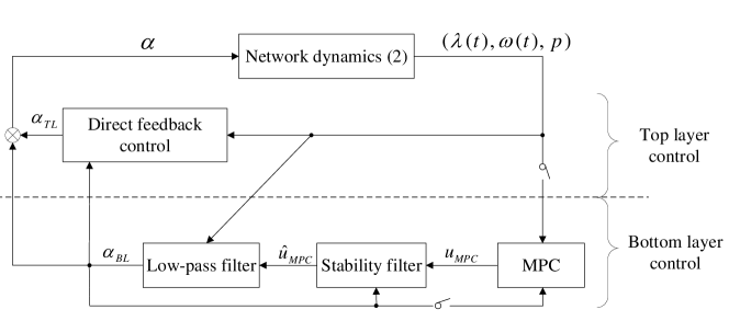
Figure 1: Block diagram of the closed-loop system with the proposed controller architecture.

IV Centralized bilayered controller

Here, we propose a centralized controller to address the requirements posed in Section III. Our idea for design starts from considering MPC to account for the economic cooperation requirement; however, MPC cannot be run continuously due to the computational burden of its online optimization. We therefore compute MPC solutions periodically. Given the reliance of the MPC implementation on sampled system states that are potentially outdated, we include additional components that employ real-time state information to tune the output of the MPC implementation and ensure stability and frequency safety. The control signal $\alpha$ is defined by

$$\alpha=\alpha_{TL}+\alpha_{BL}.$$ (5)

Roughly speaking, the bottom-layer controller $\alpha_{BL}$ periodically and optimally allocates control effort, while respecting a stability constraint and steering the frequency trajectories as a first step to achieve frequency invariance and attractivity. The top-layer controller $\alpha_{TL}$, implemented in real time, slightly tunes the control trajectory generated by the bottom layer, ensuring frequency invariance and attractivity. Figure 1 shows the overall structure of the closed-loop system. Interestingly, as we show later, the combination of the stability filter, low pass filter, and direct feedback control stabilizes the system regardless of what is in the MPC block. In the following, we provide detailed definitions of each of the design elements.

IV-A Bottom-layer controller design

We introduce here the bottom-layer control signal $\alpha_{BL}$, which results from the combination of three components, cf. Figure 1: a MPC component, a stability filter, and a low-pass filter. The MPC component periodically samples the system state, solves an optimization problem online, and updates its output signal $u_{MPC}$. The purpose of having this MPC component is to efficiently allocate control resources to achieve the frequency safety requirement. The stability filter is designed to guarantee closed-loop asymptotic stability by enforcing monotonic decrease of an appropriate energy function (which we define later). Since $\hat{u}_{MPC}$ is merely a piece-wise continuous signal, to avoid discontinuity in the control signal, the low-pass filter further smooths it to generate an input $\alpha_{BL}$ that is continuous in time. The bottom-layer controller by itself stabilizes the system (without the need of the top layer) but does not guarantee frequency safety. This is precisely the role of the top-layer design, which based on real-time system state information, slightly tunes the control signal generated by the bottom layer to achieve frequency safety while maintaining system stability. Note that, except for the MPC component, all other components can access real-time information.

Next, we introduce each component in the bottom layer and characterize their properties.

IV-A1 MPC component

Based on the most recent sampled system information, the MPC component updates its output after solving an optimization problem online. Formally, denote $\{t^{w}\}_{w\in{\mathbb{N}}}$ as the collection of sampling time instants, where $t^{w+1}>t^{w}\geqslant 0$ holds for every $w\in{\mathbb{N}}$. At each sampling time $t=t^{w}$, define a piece-wise continuous signal $p^{fcst}_{t}:[t,t+\tilde{t}]\rightarrow{\mathbb{R}}^{n}$ as the predicted value of the true power injection $p$ for the $\tilde{t}$ seconds immediately following $t$. Note that here we particularly allow the predicted power injection to be time-varying, although its true value is time-invariant. For convenience of exposition, we define

$$x\triangleq(\lambda,\omega,\alpha_{BL})$$

as the augmented collection of system states (the last state comes from the low-pass filter component). Let $x(t^{w})=(\lambda(t^{w}),\omega(t^{w}),\alpha_{BL}(t^{w}))$ be the augmented system state value at the sampling time $t^{w}$.

In the predicted model, we discretize the system dynamics with time step $T>0$, and denote $N\triangleq\lceil\tilde{t}/T\rceil$ as the predicted step length. At every $t=t^{w}$, the MPC component solves the following optimization problem,

$$\min_{\hat{X},\hat{u},S}\quad g(\hat{X},\hat{u},S)\triangleq\sum_{k=1}^{N}\Big{(}\sum_{i\in\mathcal{I}^{u}}c_{i}\hat{\alpha}_{BL,i}^{2}(k)+\sum_{i\in\mathcal{I}^{\omega}}d_{i}s_{i}^{2}(k)\Big{)}$$

s.t. $$F\hat{x}(k+1)=A\hat{x}(k)+B_{1}\hat{p}^{fcst}(k)+B_{2}\hat{u}$$ (6a)

$$\hat{u}\in\mathbb{A},$$ (6b)

$$\hat{x}(1)=x(t^{w}),$$ (6c)

$$\underline{\omega}_{i}-s_{i}(k)\leqslant\hat{\omega}_{i}(k)\leqslant\bar{\omega}_{i}+s_{i}(k),\ \forall i\in\mathcal{I}^{\omega},\forall k\in[1,N]_{{\mathbb{N}}},$$ (6d)

$$|\hat{u}_{i}|\leqslant\epsilon_{i}|\alpha_{BL,i}(t^{w})|,\quad\forall i\in\mathcal{I}^{u}.$$ (6e)

In this optimization, (6a) combines the linearized, discretized dynamics corresponding to (2) as well as the low-pass filter introduced later, and $\hat{x}\triangleq(\hat{\lambda},\hat{\omega},\hat{\alpha}_{BL})\in{\mathbb{R}}^{m+2n}$ corresponds to the predicted system state. Depending on the specific discretization method, one can choose different matrices $F$, $A\in{\mathbb{R}}^{(m+2n)\times(m+2n)}$ and $B_{1},B_{2}\in{\mathbb{R}}^{(m+2n)\times n}$ (Section IV-B below contains a detailed discussion on discretization); $\hat{p}^{fcst}_{t^{w}}(k)\triangleq p^{fcst}_{t^{w}}(t^{w}+(k-1)T)$ for every $k\in[1,N]_{{\mathbb{N}}}$; (6b) specifics the control availability for each bus; (6c) is the initial condition; (6d) represents a soft version of the frequency safety constraint, where we penalize in the cost function the deviation of predicted frequency from its desired bounds; (6e) restricts the value of the control input $\hat{u}_{i}\in{\mathbb{R}}$ with respect to the state of the low-pass filter via a tunable parameter $\epsilon_{i}>0$; finally, the objective function $g$ combines the overall cost of control effort and the penalty on the violation of the frequency safety requirement, where $c_{i}>0$ for each $i\in\mathcal{I}^{u}$ and $d_{i}>0$ for each $i\in\mathcal{I}^{\omega}$ are design parameters. For compactness, we define

$$\hat{X} \triangleq[\hat{x}(1),\hat{x}(2),\cdots,x(N)],$$ (7a)

$$S \triangleq[s(1),s(2),\cdots,s(N)],$$ (7b)

$$\hat{P}_{t^{w}}^{fcst} \triangleq[\hat{p}_{t^{w}}^{fcst}(1),\hat{p}_{t^{w}}^{fcst}(2),\cdots,\hat{p}_{t^{w}}^{fcst}(N)],$$ (7c)

where for every $k\in[1,N]_{{\mathbb{N}}}$, $s(k)$ is the collection of $s_{i}(k)$’s over $i\in\mathcal{I}^{\omega}$.

We denote by $\mathbf{R}(\mathcal{G},\mathcal{I}^{u},\mathcal{I}^{\omega},\hat{P}_{t^{w}}^{fcst},x(t^{w}))$ as the optimization problem (6) to emphasize its dependence on network topology, nodal indexes with exogenous control signals, nodal indexes with transient frequency requirement, forecasted power injection, and state values at the sampling time. We may simply use $\mathbf{R}$ if the context is clear. Also, we denote $(\hat{X}^{*},\hat{u}^{*},S^{*})$ as its optimal solution.

Remark IV.1.

(Selection of frequency violation penalty coefficient). The parameter $d=\{d_{i}\}_{i\in\mathcal{I}^{\omega}}$ in the objective function plays a fundamental rule in determining how the predicted frequency can exceed the safe bounds. In the extreme case $d=\mathbb{0}_{|\mathcal{I}^{\omega}|}$ (i.e., no penalty for frequency violation), the MPC controller loses its functionality of adjusting frequency. As $d$ grows, the controller ensures that the violation of the frequency safety requirement become smaller. The top-layer control introduced later adds additional input to the bottom-layer controller to ensure the frequency requirement is satisfied. $\bullet$

Given the open-loop optimization problem (6), the function $u_{MPC}$ corresponding to the MPC component in Figure 1 is defined as follows: for $w\in{\mathbb{N}}$ and $t\in[t^{w},t^{w+1})$, let

$$u_{MPC}(t)\!=\!\hat{u}^{*}(\mathcal{G},\mathcal{I}^{u},\mathcal{I}^{\omega},\hat{P}^{fcst}_{t^{w}},x(t^{w})).$$ (8)

Note the last two arguments that $\hat{u}^{*}$ depends on: forecasted power injection value and state value of the entire network at a sampling time. To implement (8), a straightforward idea is to have one operator globally gather the above two values, obtain $\hat{u}^{*}$ by solving $\mathbf{R}$, and finally broadcast $\hat{u}^{*}_{i}$ to the $i$th node. Later in Section V, we propose an alternative distributed computation algorithm to reduce the computational burden. The next result characterizes the dependence of the controller on the sampled state values and predicted power injection.

Proposition IV.2.

(Piece-wise affine and continuous dependence of optimal solution on sampling state and predicted power injection). Suppose $F$ is invertible, then the optimization problem $\mathbf{R}(\mathcal{G},\mathcal{I}^{u},\mathcal{I}^{\omega},\hat{P}^{fcst}_{t^{w}},x(t^{w}))$ in (6) has a unique optimal solution $(\hat{X}^{*},\hat{u}^{*},S^{*})$. Furthermore, given $\mathcal{G},\ \mathcal{I}^{u}$, and $\mathcal{I}^{\omega}$, $\hat{u}^{*}$ is continuous and piece-wise affine in $(\hat{P}_{t^{w}}^{fcst},x(t^{w}))$, that is, there exist $l\in{\mathbb{N}},\{H_{\xi}\}_{\xi=1}^{l}$, $\{K_{\xi}\}_{\xi=1}^{l}$, $\{h_{\xi}\}_{\xi=1}^{l}$, and $\{k_{\xi}\}_{\xi=1}^{l}$ with suitable dimensions such that

$$\hat{u}^{*}=K_{\xi}z+k_{\xi},\text{ if }z\in\left\{y\;|\;H_{\xi}y\leqslant h_{\xi}\right\}\text{ for }\xi\in[1,l]_{{\mathbb{N}}}$$ (9)

holds for every $z\in{\mathbb{R}}^{(N+2)n+m}$, where $z$ is the collection of $(\hat{P}_{t^{w}}^{fcst},x(t^{w}))$ in column-vector form.

Proof.

We start by noting that $\mathbf{R}$ is feasible (hence at least one optimal solution exists) for any given $z$. This is because, given a state trajectory $\hat{X}$ of (6a) with input $\hat{u}=\mathbb{0}_{n}$ and initial condition (6c), choosing a sufficiently large $s(k)$ for each $k\in[1,N]_{{\mathbb{N}}}$ makes it satisfy constraint (6d). The uniqueness follows from the facts that I) $g$ is strongly convex in $(\hat{u},S)$; II) $\hat{X}$ is uniquely and linearly determined by $\hat{u}$; III) all constraints are linear in $(\hat{X},\hat{u},S)$. To show continuity and piece-wise affinity, we separately consider $2^{|\mathcal{I}^{u}|}$ cases, depending on the sign of each $\{\alpha_{BL,i}(t^{w})\}_{i\in\mathcal{I}^{u}}$. Specifically, let $\eta\triangleq\{\eta_{i}\}_{i\in\mathcal{I}^{u}}\in\{1,-1\}^{|\mathcal{I}^{u}|}$ and define $\mathfrak{B}^{\eta}\triangleq\left\{z\big{|}(-1)^{\eta_{i}}\alpha_{BL,i}(t^{w})\geqslant 0,\ \forall i\in\mathcal{I}^{u}\right\}$. Note that every $z$ lies in at least one of these sets and that, in any $\mathfrak{B}^{\eta}$, the sign of each $\alpha_{BL,i}(t^{w})$ with $i\in\mathcal{I}^{u}$ is fixed. Hence all the $|\mathcal{I}^{u}|$ constraints in (6e) can be transformed into one of the following forms

$$-\epsilon_{i}\alpha_{BL,i}(t^{w}) \leqslant\hat{u}_{i}\leqslant\epsilon_{i}\alpha_{BL,i}(t^{w}) \text{if }\alpha_{BL,i}(t^{w})\geqslant 0,$$ (10a)

$$\epsilon_{i}\alpha_{BL,i}(t^{w}) \leqslant\hat{u}_{i}\leqslant-\epsilon_{i}\alpha_{BL,i}(t^{w}) \ \text{if }\alpha_{BL,i}(t^{w})\leqslant 0.$$ (10b)

Note that if $\alpha_{BL,i}(t^{w})=0$, then $\hat{u}_{i}=0$. Therefore, in every $\mathfrak{B}^{\eta}$, $z$ appears in $\mathbf{R}$ in a linear fashion; hence, it is easy to re-write $\mathbf{R}$ into the following form:

$$\min_{q} q^{T}Vq$$

s.t. $$Gq\leqslant W+J^{\eta}z,$$ (11)

where $q$ is the collection of $(\hat{X},\hat{u},S)$ in vector form and $V\succeq 0$, $G$, $W$ and $J^{\eta}$ are matrices with suitable dimensions. Note that only $J^{\eta}$ depends on $\eta$. By [21, Theorem 1.12], for every $\eta\in\{-1,1\}^{|\mathcal{I}^{u}|}$, $s^{*}$ is a continuous and piece-wise affine function of $z$ whenever $z\in\mathfrak{B^{\eta}}$. Since each $\mathfrak{B^{\eta}}$ consists of only linear constraints and the union of all $\mathfrak{B^{\eta}}$’s with $\eta\in\{1,-1\}^{|\mathcal{I}^{u}|}$ is ${\mathbb{R}}^{(N+2)n+m}$, one has that $s^{*}$ is piece-wise affine in $z$ on ${\mathbb{R}}^{(N+2)n+m}$. Lastly, to show the continuous dependence of $s^{*}$ on $z$ on ${\mathbb{R}}^{(N+2)n+m}$, note that since such a dependence holds on every closed set $\mathfrak{B^{\eta}}$, we only need to prove that $s^{*}$ is unique for every $z$ lying on the boundary shared by different $\mathfrak{B^{\eta}}$’s. This holds trivially as $s^{*}$ is unique for every $z\in{\mathbb{R}}^{(N+2)n+m}$, which we have proven above. ∎

Notice that the continuity and piece-wise affinity established in Proposition IV.2 together suffice to ensure that $\hat{u}^{*}$ is globally Lipschitz in $z$, and hence in the sampled system state. To see this point, one can easily check that $\max_{\xi\in[1,l]_{{\mathbb{N}}}}\|K_{\xi}\|$ qualifies as a global Lipschitz constant.

In addition, Proposition IV.2 also suggests an alternative to directly solve $\mathbf{R}$ without treating it as an optimization problem. Specifically, we can first compute and store $\{H_{\xi}\}_{\xi=1}^{l}$, $\{K_{\xi}\}_{\xi=1}^{l}$, $\{h_{\xi}\}_{\xi=1}^{l}$, and $\{k_{\xi}\}_{\xi=1}^{l}$, and then compute $\hat{u}^{*}$ online via (9). However, such an approach, usually called explicit MPC [22], suffers from the curse of dimensionality, in that the number of regions $l$ grows exponentially fast in $m+n$, input size $|\mathcal{I}^{u}|$, and horizon length $N$.

IV-A2 Stability and low-pass filters

Here we introduce the stability and low-pass filters, explain the motivation behind their definitions and characterize their properties. Note that the sampling mechanism used for the MPC component inevitably introduces delays in the bottom layer. Specifically, for any time $t\in(t^{w},t^{w+1})$, i.e., between two adjacent sampling times, $u_{MPC}(t)$ is fully determined by the old sampled system information at time $t^{w}$, as opposed to the current information. To eliminate the potential negative effect of delay on system stability, we introduce a stability filter to enforce closed-loop stability. The low-pass filter after the stability filter simply smooths the output of the stability filter to ensure that the output of the bottom layer is continuous in time. Formally, for every $i\in\mathcal{I}$ at any $t\geqslant 0$, define the stability filter as

$$\hat{u}_{MPC,i}(\alpha_{BL}(t),u_{MPC}(t))$$

$$=\operatorname{sat}(u_{MPC,i}(t);\epsilon_{i}|\alpha_{BL,i}(t)|,-\epsilon_{i}|\alpha_{BL,i}(t)|),$$ (12)

and define the low-pass filter as

$$\dot{\alpha}_{BL,i}(t) =-\frac{1}{\tau_{i}}\alpha_{BL,i}(t)-\omega_{i}(t)+\hat{u}_{MPC,i}(t),\quad\forall i\in\mathcal{I}^{u},$$

$$\alpha_{BL,i} \equiv 0,\quad\forall i\in\mathcal{I}\backslash\mathcal{I}^{u},$$ (13)

where the tunable parameter $\tau_{i}\in{\mathbb{R}}_{>}$ determines the bandwidth of the low-pass filter. In addition, although for compactness we define a stability filter for every $i\in\mathcal{I}$, one can easily see that $\hat{u}_{MPC,i}\equiv 0$ for every $i\in\mathcal{I}\backslash\mathcal{I}^{u}$.

Both the stability and the low-pass filters possess a natural distributed structure: for each $i\in\mathcal{I}^{u}$, $\alpha_{BL,i}$ only depends $\omega_{i}$ and $\hat{u}_{MPC,i}$, where the latter one only depends on $u_{MPC,i}$ and $\alpha_{BL,i}$. This implies that to implement $\hat{u}_{MPC,i}$ and $\alpha_{BL,i}$, it only requires local information at node $i$. Throughout the rest of the paper, we interchangeably use $\hat{u}_{MPC,i}(\alpha_{BL}(t),u_{MPC}(t))$ and $\hat{u}_{MPC,i}(t)$ for simplicity.

The next result establishes that $\hat{u}_{MPC}$ is Lipschitz continuous in the system state and an important property of the bottom-layer controller $\alpha_{BL}$ that we use later to establish stability.

Lemma IV.3.

(Lipschitz continuity and stability condition). For the signal $\hat{u}_{MPC}$ defined in (IV-A2), $\hat{u}_{MPC}$ is Lipschitz in system state at every sampling time $t=t^{w}$ with $w\in{\mathbb{N}}$. Furthermore, if $\alpha_{TL}$ is Lipschitz in system state, then both $\alpha_{TL}$ and $\alpha_{BL}$ are continuous in time. Additionally,

$$\alpha_{BL,i}(t)\hat{u}_{MPC,i}(t)\leqslant\epsilon_{i}\alpha_{BL,i}^{2}(t),\quad\forall t\geqslant 0,\ \forall i\in\mathcal{I}.$$ (14)

Proof.

If $t=t^{w}$, then since $|\hat{u}_{i}^{*}|\leqslant\epsilon_{i}|\alpha_{BL,i}(t^{w})|$ by (6e) and $u_{MPC,i}(t^{w})=\hat{u}_{i}^{*}$ for every $i\in\mathcal{I}^{u}$, using (IV-A2) we deduce that $\hat{u}_{MPC,i}(\alpha_{BL}(t),u_{MPC}(t))|_{t=t^{w}}=\hat{u}_{i}^{*}$. The Lipschitz continuity follows by Proposition IV.2. To show the time-domain continuity, since $\hat{u}_{MPC}$ is Lipschitz at every sampling point and the top-layer controller is also Lipschitz by hypothesis (we demonstrate this point later in Section IV-C), one has that the solutions of both $\alpha_{TL}$ and the closed-loop system (2) exist and are unique and continuous in time. Note that $u_{MPC}$ in (8) is defined to be a piece-wise constant signal. One has, by (IV-A2), that $\hat{u}_{MPC}$ is piece-wise continuous, which further makes $\alpha_{BL}$ a continuous signal in time due to the low-pass filter. Condition (14) simply follows from the definition of saturation function. ∎

Remark IV.4.

(Link between designs of the MPC component and stability filter). Note that, regardless of the MPC component output $u_{MPC}$, the output of the stability filter $\hat{u}_{MPC}$ defined in (IV-A2) always meets condition (14). This implies that any inaccuracy in the MPC component (e.g., errors in sampled state measurement, forecasted power injection, or system parameters) cannot cause instability. However, to ensure the Lipschitz continuity in Lemma IV.3, we formulate constraint (6e) employing the same coefficient $\epsilon_{i}$ in the stability filter (IV-A2). It is in this sense that both are linked. $\bullet$

Remark IV.5.

(Continuous versus periodic sampling in the MPC component). Note that if the MPC component were to sample the system state in a continuous fashion instead, then the constraint (6e) would ensure that the output of the MPC component already satisfies the stability condition (14), and hence there would be no need for the stability filter. In this regard, the role of the stability filter is to filter out the unstable parts in $u_{MPC}$ caused by non-continuous sampling. $\bullet$

IV-B Discretization with sparsity preservation

As we have introduced the dynamics of the low-pass and stability filters, we are now able to explicitly explain the computation of matrices $F$, $A$, $B_{1}$ and $B_{2}$ in the prediction model (6a). We first construct a continuous-time linear model by neglecting the top-layer controller and the stability filter ($\alpha\approx\alpha_{BL}$ and $\hat{u}_{MPC}\approx u_{MPC}$), and then linearizing the nonlinear dynamics in Figure 1. Our second step consists of appropriately discretizing this linear model.

Notice that the transformation from a nonlinear continuous-time nonlinear model to a discrete one does not affect closed-loop system stability due to the presence of the stability filter. In fact, any prediction model in the MPC component cannot jeopardize stability (cf. Remark IV.4). On the other hand, such a model simplification is reasonable since $\alpha_{BL}$ is designed to only slightly tune the control signal, and we have described in Remark IV.5 how the stability filter barely changes its input.

We obtain the linear model by assuming $\alpha\approx\alpha_{BL}$ and $\hat{u}_{MPC}\approx u_{MPC}$, and approximating the dynamics in Figure 1 by

$$\dot{\lambda}(t) =D\omega(t),$$

$$M\dot{\omega}(t) =-E\omega(t)-D^{T}Y_{b}\lambda(t)+p+\alpha_{BL}(t),$$

$$M_{i}\dot{\alpha}_{BL,i}(t) =-\frac{1}{\tau_{i}}\alpha_{BL,i}(t)-\omega_{i}(t)+\hat{u}_{MPC,i}(t),\quad\forall i\in\mathcal{I}^{u},$$

$$\alpha_{BL,i} \equiv 0,\quad\forall i\in\mathcal{I}\backslash\mathcal{I}^{u},$$ (15)

where the first two equations come from (2) by linearizing the nonlinear sinusoid function via $\sin(Y_{b}\lambda(t))\approx Y_{b}\lambda(t)$. Now we re-write the above linear dynamics into the compact form,

$$\tilde{G}\dot{x}(t)=\tilde{A}x(t)+\tilde{B}_{1}p+\tilde{B}_{2}u_{MPC}(t),$$ (16)

for certain matrices $\tilde{A}$, $\tilde{B}_{1}$, and $\tilde{B}_{2}$, with $\tilde{A}$ stable [20] and with $\tilde{G}$ a diagonal matrix whose diagonals are $1$, $M_{i}$ with $i\in[1,n]_{{\mathbb{N}}}$, or $0$. Additionally, one can easily check that the linearized dynamics (IV-B) and (16) preserve the locality of (2b) and (IV-A2).

We consider the following three discretization methods with step size $T>0$ to construct $F$, $A$, $B_{1}$, and $B_{2}$ matrices in (6a) approximating the continuous dynamics (16). For explanatory simplicity, we here assume $\tilde{G}$ is invertible.

1. Impulse invariant discretization:

   $$F\triangleq I_{m+2n},\ A\triangleq e^{\tilde{G}^{-1}\tilde{A}T},\ B_{s}\triangleq\int_{0}^{T}e^{\tilde{G}^{-1}\tilde{A}\tau}\text{d}\tau\tilde{B}_{s},\ s=1,2,$$ (17)

2. Forward Euler discretization:

   $$F\triangleq\tilde{G},\ A\triangleq T\tilde{A}+\tilde{G},\ B_{s}\triangleq T\tilde{B}_{s},\ s=1,2,$$ (18)

3. Backward Euler discretization:

   $$F\triangleq\tilde{G}-T\tilde{A},\ A\triangleq I_{m+2n},\ B_{s}\triangleq T\tilde{B}_{s},\ s=1,2,$$ (19)

where $F$ should be invertible for uniqueness of solution of the discretized dynamics.

Note that with a fixed $T$, the impulse invariant and backward Euler methods usually have better approximation accuracy than the forward Euler method. In fact, since all eigenvalues of $\tilde{A}$ have non-positive real part, a basic discretization requirement is that all eigenvalues of $F^{-1}A$ are in the unit circle to maintain stability. One can easily prove that the impulse invariant and backward Euler discretization always meet this requirement for any $T>0$, but the forward Euler method requires a sufficiently small $T$ to preserve stability; therefore, with a same predicted time horizon $\tilde{t}$, the forward Euler method has the largest predicted step length $N$ and hence makes the optimization problem $\mathbf{R}$ harder to solve. On the other hand, the backward Euler method might require a small enough $T$ to guarantee the invertibility of $F$, but numerically we have found this to be easily satisfiable. Therefore, we set aside the forward Euler method from our considerations of discretization. On the other hand, the impulse invariant method fails to preserve the sparsity of $\tilde{A}$, $\tilde{B}_{1}$, and $\tilde{B}_{2}$, which are essential for the design of distributed solvers of $\mathbf{R}$. Instead, the matrices $F$, $A$, $B_{1}$ and $B_{2}$ resulting from the backward Euler discretization are all sparse. This justifies our choice, throughout the rest of the paper, of the backward Euler method for discretization.

IV-C Top-layer controller design

In this section we describe the top-layer controller. By design, cf. (6), the bottom-layer controller makes a trade-off between the control cost and the violation of frequency safety, and hence does not strictly guarantee the latter. This is precisely the objective of the top-layer controller: ensuring frequency safety at all times by slightly adjusting, if necessary, the effect of the bottom-layer controller. Formally, for every $i\in\mathcal{I}^{\omega}$, let $\bar{\gamma}_{i},\underline{\gamma}_{i}>0$, and $\underline{\omega}_{i}^{\text{thr}},\bar{\omega}_{i}^{\text{thr}}\in{\mathbb{R}}$ with $\underline{\omega}_{i}\char 60\relax\underline{\omega}_{i}^{\text{thr}}\char 60\relax 0\char 60\relax\bar{\omega}_{i}^{\text{thr}}\char 60\relax\bar{\omega}_{i}$. We use the design from [13] for the top layer. For $i\in\mathcal{I}^{\omega}$, $\alpha_{TL,i}(x(t),p)$ takes the form

$$\begin{cases}\min\{0,\frac{\bar{\gamma}_{i}(\bar{\omega}_{i}-\omega_{i}(t))}{\omega_{i}(t)-\bar{\omega}_{i}^{\text{thr}}}+v_{i}(x(t),p)\}&\omega_{i}(t)>\bar{\omega}_{i}^{\text{thr}},\\ 0&\underline{\omega}_{i}^{\text{thr}}\leqslant\omega_{i}(t)\leqslant\bar{\omega}_{i}^{\text{thr}},\\ \max\{0,\frac{\underline{\gamma}_{i}(\underline{\omega}_{i}-\omega_{i}(t))}{\underline{\omega}_{i}^{\text{thr}}-\omega_{i}(t)}+v_{i}(x(t),p)\}&\omega_{i}(t)\char 60\relax\underline{\omega}_{i}^{\text{thr}},\end{cases}$$ (20)

where

$$v_{i}(x(t),p) \triangleq E_{i}\omega_{i}(t)+[D^{T}]_{i}\sin(Y_{b}\lambda(t))-p_{i}-\alpha_{BL,i}(t),$$

and for $i\in\mathcal{I}\backslash\mathcal{I}^{\omega}$, simply $\alpha_{TL,i}\equiv 0$. The top-layer controller can be implemented in a decentralized fashion: for each $\alpha_{TL,i}$ with $i\in\mathcal{I}^{\omega}$ on bus $i$, its implementation only requires the bus frequency $\omega_{i}$, aggregated power flow $[D^{T}]_{i}\sin(Y_{b}\lambda)$, power injection $p_{i}$, and $i$th component of the bottom-layer signal $\alpha_{BL,i}$, all of which are local to bus $i$. Additionally, similarly to [13], one can show that $\alpha_{TL}$ is locally Lipschitz in $x$. For brevity, we may use $\alpha_{TL,i}(x(t),p)$ (respectively, $v_{i}(x(t),p)$) and $\alpha_{TL,i}(t)$ (respectively $v_{i}(t)$) interchangeably.

Each $\alpha_{TL,i}$, with $i\in\mathcal{I}^{\omega}$, behaves as a passive and myopic transient frequency regulator without prediction capabilities. We offer the following observations about its definition: first, $\alpha_{TL,i}$ only depends on local system information and does not incorporate any global knowledge; second, $\alpha_{TL,i}$ vanishes as long as the current frequency is within $[\underline{\omega}_{i}^{\text{thr}},\bar{\omega}_{i}^{\text{thr}}]$, a subset of the safe frequency interval, with no consideration for the possibility of future large disturbances; third, $\alpha_{TL,i}$ can be non-zero when the current frequency is out of $[\underline{\omega}_{i}^{\text{thr}},\bar{\omega}_{i}^{\text{thr}}]$ and hence close to the safe frequency boundaries. However, this could also lead to over-reaction, especially when $\bar{\gamma}_{i}$ and $\underline{\gamma}_{i}$ are small, as the disturbance may disappear suddenly, in which case even without the top-layer controller, the frequency would remain safe afterwards. As pointed out above, the top-layer controller only steps in if the input from the bottom-layer controller is not sufficient to ensure frequency safety.

IV-D Frequency safety and local asymptotic stability

Having introduced the elements of both layers in Figure 1, we are now ready to show that the proposed centralized control strategy meets requirements (i)-(iv) in Section III. We focus on the first two requirements, since we have already established the Lipschitz continuity of each individual component, and the MPC component by design takes care of the economic cooperation among the controlled buses.

For the open-loop system (2) with $\alpha\equiv 0_{n}$, under condition (4), the following energy function [7] is identified to prove local asymptotic stability and estimate the region of attraction,

$$V(x)\triangleq\frac{1}{2}\sum_{i=1}^{\bar{n}}M_{i}\omega_{i}^{2}+\sum_{j=1}^{m}[Y_{b}]_{j,j}a(\lambda_{j}),$$ (21)

where $a(\lambda_{j})\triangleq\cos\lambda_{j}^{\infty}-\cos\lambda_{j}-\lambda_{j}\sin\lambda_{j}^{\infty}+\lambda_{j}^{\infty}\sin\lambda_{j}^{\infty}$ for every $j\in[1,m]_{{\mathbb{N}}}$. For notational simplicity, here we assume that the first $\bar{n}$ nodes have strictly positive inertia, whereas the rest $n-\bar{n}$ nodes have zero inertia. Due to the extra dynamics introduced by the low-pass filter, we here consider the following energy function for the closed-loop system,

$$\bar{V}(x)=V(x)+\frac{1}{2}\sum_{i\leqslant\bar{n},i\in\mathcal{I}^{u}}M_{i}\alpha^{2}_{BL,i}.$$ (22)

Furthermore, define the level set

$$\mathcal{T}_{\rho}\triangleq\left\{x\;\big{|}\;\lambda\in\Upsilon_{cl},\ \bar{V}(x)\leqslant\rho c\right\},$$ (23)

where $\rho\geqslant 0$ and $c\triangleq\min_{\tilde{\lambda}\in\partial\Upsilon}\bar{V}(\tilde{\lambda},\mathbb{0}_{n},\mathbb{0}_{n})$. Now we are ready to prove that system (2) with the proposed controller guarantees frequency safety and local asymptotic stability jointly.

Theorem IV.6.

(Bilayered control with stability and frequency guarantees). Under condition (4), assume that $\epsilon_{i}\tau_{i}\char 60\relax 1$ for every $i\in\mathcal{I}^{u}$, and $x(0)\in\mathcal{T}$, then the system (2) with the bilayered controller defined by (5), (8), (IV-A2), (IV-A2), and (20) satisfies

1. for any $i\in\mathcal{I}^{\omega}$, if $\omega_{i}(0)\in[\underline{\omega}_{i},\bar{\omega}_{i}]$, then $\omega_{i}(t)\in[\underline{\omega}_{i},\bar{\omega}_{i}]$ for every $t\geqslant 0$;

2. for any $i\in\mathcal{I}^{\omega}$, if $\omega_{i}(0)\notin[\underline{\omega}_{i},\bar{\omega}_{i}]$, then there exists $t_{0}$ such that $\omega_{i}(t)\in[\underline{\omega}_{i},\bar{\omega}_{i}]$ for every $t\geqslant t_{0}$. Furthermore, $\omega_{i}(t)$ monotonically approaches $[\underline{\omega}_{i},\bar{\omega}_{i}]$ before entering it;

3. if the initial state $(\lambda(0),\omega(0),\alpha_{BL}(0))$ is in $\mathcal{T}_{\rho}$ for some $0\char 60\relax\rho\char 60\relax 1$, then $(\lambda(t),\omega(t),\alpha_{BL}(t))$ stays in $\mathcal{T}_{\rho}$ for all $t>0$, and converges to $(\lambda_{\infty},\mathbb{0}_{n},\mathbb{0}_{n})$. Furthermore, $\alpha(t)$, $\alpha_{TL}(t)$, $\alpha_{BL}(t)$, $\hat{u}_{MPC}(t)$, and $u_{MPC}(t)$ all converge to $\mathbb{0}_{n}$ as $t\rightarrow\infty$.

Proof.

It is easy to see that statement (i) is equivalent to asking that, for any $i\in\mathcal{I}^{\omega}$ at any $t\geqslant 0$,

$$\dot{\omega}_{i}(t)\leqslant 0\text{ if }\omega_{i}(t)=\bar{\omega}_{i},$$ (24a)

$$\dot{\omega}_{i}(t)\geqslant 0\text{ if }\omega_{i}(t)=\underline{\omega}_{i}.$$ (24b)

For simplicity, we only prove (24a), and (24b) follows similarly. Note that by (2b), (5), and (20), one has

$$M_{i}\dot{\omega}_{i}(t) =-E_{i}\omega_{i}(t)-[D^{T}]_{i}\sin(Y_{b}\lambda(t))+p_{i}+\alpha_{i}(t)$$

$$=-E_{i}\omega_{i}(t)-[D^{T}]_{i}\sin(Y_{b}\lambda(t))+p_{i}+\alpha_{BL,i}(t)+\alpha_{TL,i}(t)$$

$$=-v_{i}(t)+\alpha_{TL,i}(t).$$ (25)

$\omega_{i}(t)=\bar{\omega}_{i}$, then $-v_{i}(t)+\alpha_{TL,i}(t)=-v_{i}(t)+\min\{0,v_{i}(t)\}\leqslant 0$; hence condition (24a) holds for every $i\in\mathcal{I}^{\omega}$ with $M_{i}>0$.

To establish the result for the case when $M_{i}=0$, we reason as follows. Starting from the last line of (IV-D), the following holds when $\omega_{i}(t)>\bar{\omega}_{i}^{\text{thr}}$,

$$E_{i}\omega_{i}(t) =E_{i}\omega_{i}(t)-v_{i}(t)+\alpha_{TL,i}(t)$$

$$=\min\{E_{i}\omega_{i}(t)-v_{i}(t),E_{i}\omega_{i}(t)+\frac{\bar{\gamma}_{i}(\bar{\omega}_{i}-\omega_{i}(t))}{\omega_{i}(t)-\bar{\omega}_{i}^{\text{thr}}}\}$$

$$\leqslant E_{i}\omega_{i}(t)+\frac{\bar{\gamma}_{i}(\bar{\omega}_{i}-\omega_{i}(t))}{\omega_{i}(t)-\bar{\omega}_{i}^{\text{thr}}},$$

and hence $\frac{\bar{\gamma}_{i}(\bar{\omega}_{i}-\omega_{i}(t))}{\omega_{i}(t)-\bar{\omega}_{i}^{\text{thr}}}\geqslant 0$, implying that $\omega_{i}(t)\leqslant\bar{\omega}_{i}$. Similarly, one can prove that $\omega_{i}(t)\geqslant\underline{\omega}_{i}$ for every $t\geqslant 0$.

Note that (ii) follows from (i) and (iii). This is because, for any $i\in\mathcal{I}$, if $\omega_{i}$ converges to $0\in(\underline{\omega}_{i},\bar{\omega}_{i})$, there must exist a finite time $t_{0}$ such that $\omega_{i}(t_{0})\in[\underline{\omega}_{i},\bar{\omega}_{i}]$, which, by (i), implies that $\omega_{i}(t)\in[\underline{\omega}_{i},\bar{\omega}_{i}]$ at any $t\geqslant t_{0}$. We then prove statement (iii), To show the invariance of $\mathcal{T}_{\rho}$, first, it is easy to see that $c>0$ by noticing that $\lambda_{\infty}\not\in\partial\Upsilon$, and $V(\tilde{\lambda},\mathbb{0}_{n},\mathbb{0}_{n})$ is non-negative, equaling 0 if and only if $\tilde{\lambda}=\lambda_{\infty}$. Next, we show that $\dot{\bar{V}}\leqslant 0$ for every $x\in\mathcal{T}_{\rho}$. We obtain after some computations that

$$\dot{\bar{V}}= -\omega^{T}(t)E\omega(t)+\sum_{i\leqslant\bar{n},i\in\mathcal{I}^{\omega}}\omega_{i}(t)\alpha_{TL,i}(t)$$

$$-\sum_{,i\in\mathcal{I}^{u}}\left(\frac{1}{\tau_{i}}\alpha_{BL,i}^{2}(t)-\alpha_{BL,i}(t)\hat{u}_{MPC,i}(t)\right).$$

Note that by the definition of $\alpha_{TL}$ in (20), $\omega_{i}(t)\alpha_{TL,i}(t)\leqslant 0$ holds for every $i\in\mathcal{I}^{\omega}$ at every $t\geqslant 0$, in that $\alpha_{TL,i}(t)=0$ whenever $\underline{\omega}_{i}^{\text{thr}}\leqslant\omega_{i}(t)\leqslant\bar{\omega}_{i}^{\text{thr}}$, and $\alpha_{TL,i}(t)\geqslant 0$ (reps. $\leqslant 0$) if $\omega_{i}(t)\geqslant\bar{\omega}_{i}^{\text{thr}}>0$ (respectively, $\omega_{i}(t)\leqslant\underline{\omega}_{i}^{\text{thr}}\char 60\relax 0$). Therefore, together with condition (14) in Lemma IV.3, we have

$$\dot{\bar{V}}\leqslant-\omega^{T}(t)E\omega(t)-\sum_{i\in\mathcal{I}^{u}}(\frac{1}{\tau_{i}}-\epsilon_{i})\alpha_{BL,i}^{2}(t)\leqslant 0,$$ (26)

and hence $\bar{V}(x(t))\leqslant\rho c$ for all $t\geqslant 0$. Finally, by the definition of $c$, one can check that $\lambda$ stays in $\Upsilon_{\text{cl}}$ all the time, otherwise there exists some $t\geqslant 0$ such that $\lambda(t)\in\partial\Upsilon$, resulting in $\bar{V}(x(t))\geqslant c>\rho c$. Therefore, the set $\mathcal{T}_{\rho}$ is invariant.

The convergence of state follows by LaSalle Invariance Principle [12, Theorem 4.4]. Specifically, $\omega(t)$ and $\alpha_{BL}(t)$ converge to $\mathbb{0}_{n}$ (notice that $\alpha_{BL,i}\equiv 0$ for each $i\in\mathcal{I}\backslash\mathcal{I}^{u}$). Next we show that $\lim_{t\rightarrow\infty}\alpha_{TL,i}(t)=0$ for every $i\in\mathcal{I}^{\omega}$, which implies that $\lim_{t\rightarrow\infty}\alpha_{TL}(t)=\mathbb{0}_{n}$ as $\alpha_{TL,i}\equiv 0$ for each $i\in\mathcal{I}\backslash\mathcal{I}^{\omega}$. This simply follows from (20) since $\alpha_{TL,i}(t)=0$ whenever $\underline{\omega}_{i}^{\text{thr}}\leqslant\omega_{i}(t)\leqslant\bar{\omega}_{i}^{\text{thr}}$, where $0\in(\underline{\omega}_{i}^{\text{thr}},\bar{\omega}_{i}^{\text{thr}})$, and we have shown that $\lim_{t\rightarrow\infty}\omega(t)=\mathbb{0}_{n}$. The convergence of $\alpha(t)$ follows from its definition (5). Since (IV-A2) implies that $|\hat{u}_{MPC,i}(t)|\leqslant\epsilon_{i}|\alpha_{BL,i}(t)|$ for every $i\in\mathcal{I}$ at every $t\geqslant 0$, one has $\lim_{t\rightarrow\infty}\hat{u}_{MPC}(t)=\mathbb{0}_{n}$. Finally, since $\hat{u}^{*}(\mathcal{G},\mathcal{I}^{u},\mathcal{I}^{\omega},\hat{P}^{fcst}_{t^{w}},x(t^{w}))$ is the optimal solution of the optimization problem (6), it must satisfy constraint (6e), and since $\lim_{w\rightarrow\infty}\alpha_{BL}(t^{w})=\lim_{t\rightarrow\infty}\alpha_{BL}(t^{t})=\mathbb{0}_{n}$, one has $\lim_{w\rightarrow\infty}\hat{u}^{*}(\mathcal{G},\mathcal{I}^{u},\mathcal{I}^{\omega},\hat{P}^{fcst}_{t^{w}},x(t^{w}))=\mathbb{0}_{n}$. Finally, the convergence of $u_{MPC}(t)$ follows from its definition (8). ∎

Since the MPC component cannot jeopardize system closed-loop asymptotic stability, cf. Remark IV.4, as one can see in the proof of Theorem IV.6(iii), the convergence of $\lambda(t)$, $\omega(t)$, $\alpha_{BL}(t)$, $\alpha(t)$, $\alpha_{TL}(t)$, $\alpha_{BL}(t)$, and $\hat{u}_{MPC}(t)$ does not require any a priori assumption on the output $u_{MPC}(t)$ of the MPC component. In the simulations, we show that even if we perturb $u_{MPC}(t)$ by intentionally shifting its output from its true value by a constant, the convergence of the remaining signals still holds. On the other hand, the convergence of $u_{MPC}(t)$ depends on the convergence of $\alpha_{BL}(t)$. In addition, since both $\hat{u}_{MPC}(t)$ and $u_{MPC}(t)$ converge to $\mathbb{0}_{n}$ (and so does their difference), we also conclude that the stability filter ultimately lets the MPC component output signal pass, i.e., the stability filter preserves the optimality of the MPC component in the long run.

One can also verify the independence between stability and the MPC component by noting that all stability results of Theorem IV.6 do not rely on any assumption on the forecasted power injection. Although the MPC component is a full-state feedback, due to this independence, Theorem IV.6 still holds if the measured state is delayed or inaccurate. This means that one could instead employ an output feedback controller by designing a state observer and feeding the estimated state into the MPC component without endangering stability. The minimal set of measured information required to realize the controller are: $\omega_{i}$, $\alpha_{BL,i}$, $[D^{T}]_{i}\sin(Y_{b}\lambda)$, and $p_{i}$ for every $i\in\mathcal{I}^{\omega}$. This information is used in the stability and low-pass filters, and the top-layer controller. Of course, inaccurate state and forecasted power injection lead to non-optimal control commands in the MPC component and higher cost.

Remark IV.7.

(Frequency safety with time-varying power injection). If the power injection is time-varying, one can see from the proof of Theorem IV.6 that (i) still holds and (ii) partially holds, in the sense that the frequency would approach the safe interval but may not enter it within a finite time. $\bullet$

Remark IV.8.

(Independence of controller on equilibrium point). It should be pointed out that in Theorem IV.6, the proposed controller is able to locally stabilize the system without a priori knowledge on the steady-state voltage angle $\lambda_{\infty}$. Specifically, both $\alpha_{BL}$ and $\alpha_{TL}$ are not functions of $\lambda_{\infty}$. $\bullet$

Remark IV.9.

(Control framework without bottom layer). In our previous work [13], we have shown that the top-layer controller by itself makes the closed-loop system meet all requirements except for the economic cooperation. Such a lack of cooperation can be observed in two aspects. First, since $\alpha_{TL}$ is only defined for nodes in $\mathcal{I}^{\omega}$, those in $\mathcal{I}^{u}\backslash\mathcal{I}^{\omega}$ do not get involved in controlling frequency transients. Second, the top-layer control is a non-optimization-based state feedback, where each $\alpha_{TL,i}$ with $i\in\mathcal{I}^{\omega}$ is merely in charge of controlling the transient frequency for its own node $i$. $\bullet$

V Controller decentralization

The centralized bilayered controller meets the requirements (i)-(iv) stated in Section III. In this section, we focus on the requirement (v) on the distributed implementation of the controller. While introducing each controller component in Figure 1, our discussion has shown that only the MPC component requires access to global system information, whereas all other components can be implemented in a distributed fashion. In this section, we show that by having each node and edge communicate within its 2-hop neighbors, one can solve the optimization problem $\mathbf{R}$ in (6) online and hence exactly recover the MPC component $\hat{u}^{*}$ in (8). The key idea is to properly assign the decision variables in the optimization problem to each node so that the cost function can be represented as sum of local costs and the constraints can be written locally. Once this is in place, we report to saddle-point dynamics to find the solution of $\mathbf{R}$ in a distributed way.

V-A Strong convexification of the objective function

We start here by transforming the optimization problem $\mathbf{R}$ into an equivalent form whose objective function is strongly convex in all its arguments. Such property is useful later when characterizing the convergence properties of distributed algorithm to the optimizer. Formally, let

$$g^{\text{aug}}(\hat{X},\hat{u},S) \triangleq\sum_{k=1}^{N-1}\|F\hat{x}(k+1)-A\hat{x}(k)-B_{1}\hat{p}^{fcst}(k)-B_{2}\hat{u}\|_{2}^{2}$$

$$\quad+\sum_{k=1}^{N}\left(\sum_{i\in\mathcal{I}}c_{i}\hat{\alpha}_{BL,i}^{2}(k)+\sum_{i\in\mathcal{I}^{\omega}}d_{i}s_{i}^{2}(k)\right)$$ (27)

$$\quad+\|\hat{x}(0)-x(t^{w})\|_{2}^{2}.$$

We denote by $\mathbf{R}^{\text{aug}}$ the optimization problem with objective function $g^{\text{aug}}$ and constraints given by (6a)-(6e). Letting $Y\triangleq(\hat{X},\hat{u},S)\in{\mathbb{R}}^{(m+2n+|\mathcal{I}^{\omega}|)N+n}$, we can re-write $\mathbf{R}^{\text{aug}}$ into the following compact form

$$\min_{Y}\frac{1}{2}Y^{T}HY+f^{T}Y+a$$

s.t. $$R_{1}Y\leqslant r_{1},$$ (28a)

$$R_{2}Y=r_{2},$$ (28b)

for suitable

$$H \in{\mathbb{R}}^{((m+2n+|\mathcal{I}^{\omega}|)N+n)\times((m+2n+|\mathcal{I}^{\omega}|)N+n)},$$

$$f \in{\mathbb{R}}^{(m+2n+|\mathcal{I}^{\omega}|)N+n},\qquad a\in{\mathbb{R}},$$

$$R_{1} \in{\mathbb{R}}^{(2|\mathcal{I}^{\omega}|N+2|\mathcal{I}^{u}|)\times((m+2n+|\mathcal{I}^{\omega}|)N+n)},$$

$$R_{2} \in{\mathbb{R}}^{((m+2n)N+n-|\mathcal{I}^{u}|)\times((m+2n+|\mathcal{I}^{\omega}|)N+n)},$$

$$r_{1} \in{\mathbb{R}}^{2|\mathcal{I}^{\omega}|N+2|\mathcal{I}^{u}|},\qquad r_{2}\in{\mathbb{R}}^{(m+2n)N+n-|\mathcal{I}^{u}|}.$$

The next result shows the equivalence between $\mathbf{R}$ and $\mathbf{R}^{\text{aug}}$.

Lemma V.1.

(Equivalent transformation to strong convexity). The optimization problem $\mathbf{R}$ and $\mathbf{R}^{\text{aug}}$ posses exactly the same optimal solution. Furthermore, if $F$ is invertible, then $g^{\text{aug}}$ is strongly convex in $(\hat{X},\hat{u},S)$.

Proof.

The equivalence between $\mathbf{R}$ and $\mathbf{R}^{\text{aug}}$ follows by noting that $g^{\text{aug}}$ corresponds to augmenting $g$ with equality constraints. For notational simplicity, we assume that $c_{i}=1$ for all $i\in\mathcal{I}$ and $d_{i}=1$ for all $i\in\mathcal{I}^{\omega}$ (the proof holds for general positive values with minor modifications). To show strong convexity, one can write $H$ as an upper-triangular block matrix, whose diagonal matrices are $F^{T}F+J^{T}J$, $F^{T}F+A^{T}A+J^{T}J$, $A^{T}A+J^{T}J$, $B_{2}^{T}B_{2}$, and $I_{|\mathcal{I}^{\omega}|N}$, where $J\in{\mathbb{R}}^{(m+2n)\times n}$ is a matrix mapping the whole state $\hat{x}$ to the partial state $\hat{\alpha}_{BL}$, i.e., $\hat{\alpha}_{BL}=J\hat{x}$. It is easy to see that both $J$ and $B_{2}$ are full-column-rank matrices, which, together with the invertibility assumption on $F$, implies that all five matrices are positive definite. Hence, all eigenvalues of $H$ are real and strictly positive, leading to strong convexity of $g^{aug}$, as claimed. ∎

V-B Separable objective with locally expressible constraints

Next, we explain how the problem data defining the optimization $\mathbf{R}^{\text{aug}}$ has a structure that makes it amenable to distributed algorithmic solutions. We start by assigning the decision variables $Y=(\hat{X},\hat{u},S)$ in $\mathbf{R}^{\text{aug}}$ to the nodes and edges in the network. We partition the states into voltage angle difference, frequency, and low-pass filter state, i.e., $\hat{x}=(\hat{\lambda},\hat{\omega},\hat{\alpha}_{BL})$. For every $k\in[0,N]_{{\mathbb{N}}}$, $i\in[1,n]_{{\mathbb{N}}}$, and $j\in[1,m]_{{\mathbb{N}}}$, we assign $\omega_{i}(k)$, $\hat{u}_{i}$, and $\hat{\alpha}_{BL,i}(k)$ to the $i$th node, and $\hat{\lambda}_{j}(k)$ to the $j$th edge. For every $i\in\mathcal{I}^{\omega}$, we assign $s_{i}(k)$ to the $i$th node. In the subsequent discussion, we say a constraint or function is local for the power network $\mathcal{G}$ if its decision variables are all from either of the following two cases: a) a node $i\in\mathcal{I}$ and its neighboring edges $(i,j)\in\mathcal{E}$, and b) an edge $(i,j)\in\mathcal{E}$ and its neighboring nodes $i$ and $j$. We claim that

1. if $F$, $A$, $B_{1}$ and $B_{2}$ are determined by (19), then every constraint in (6) is local.

2. the objective function $g^{\text{aug}}$ can be written as a sum of local objective functions.

To see (i), note that (6b)-(6e) are a collection of constraints, each depending only on variables owned by a single node. Constraint (6a) is also local by noticing the following two points. First, the dynamics of each state in (IV-B) is uniquely determined by the states of its neighbors. Second, we have shown in Section IV-B that the backward Euler discretization (19) preserves locality. To see (ii), first note that the sum of $\alpha_{BL,i}^{2}(k)$ (respectively, $s_{i}^{2}(k)$) over $i$ is naturally the sum of local variables. Second, the two-norm square of $F\hat{x}(k+1)-A\hat{x}(k)-B_{1}\hat{p}^{fcst}(k)-B_{2}\hat{u}$ for every $k\in[1,N-1]_{{\mathbb{N}}}$ is the sum of square of all its $m+2n$ entries, where each entry is local due to the locality of discretized dynamics. Similarly, $\|\hat{x}(0)-x(t^{w})\|_{2}^{2}$ is also the sum of local variables.

V-C Distributed implementation via saddle-point dynamics

Here we introduce a saddle-point dynamics to recover the unique optimal solution $Y^{*}$ of $\mathbf{R}^{\text{aug}}$ in a distributed fashion. We start from the Lagrangian of $\mathbf{R}^{\text{aug}}$

$$\mathfrak{L}(Y,\eta,\mu)=g^{\text{aug}}(Y)+\eta^{T}(R_{1}Y-r_{1})+\mu^{T}(R_{2}Y-r_{2}),$$ (29)

where $\eta\in{\mathbb{R}}^{2|\mathcal{I}^{\omega}|N+2|\mathcal{I}^{u}|}_{\geqslant 0}$ and $\mu\in{\mathbb{R}}^{(m+2n)N+n-|\mathcal{I}^{u}|}$ are the Lagrangian multiplier corresponding to constraints (28a) and (28b), respectively. Note that we have shown that a) $\mathbf{R}$ is feasible (cf. Proposition IV.2), b) $\mathbf{R}$ and $\mathbf{R}^{\text{aug}}$ are equivalent (cf. Lemma V.1), and c) all constraints in $\mathbf{R}^{\text{aug}}$ are linear. These three points together imply that the refined Slater condition and strong duality hold, [23, Section 5.2.3], which further implies that at least one primal-dual solution $(Y^{*},\eta^{*},\mu^{*})$ of $\mathbf{R}^{\text{aug}}$ exists, and the set of primal-dual solutions is exactly the set of saddle points of $\mathfrak{L}$ on the set ${\mathbb{R}}^{(m+2n+|\mathcal{I}^{\omega}|)N+n}\times({\mathbb{R}}^{2|\mathcal{I}^{\omega}|N+2|\mathcal{I}^{u}|}_{\geqslant 0}\times{\mathbb{R}}^{(m+2n)N+n-|\mathcal{I}^{u}|})$ [23, Section 5.4.2]. Therefore, one can apply the saddle-point dynamics [24] to recover one solution $(Y^{*},\eta^{*},\mu^{*})$, where $\hat{u}^{*}$ is the MPC output signal we need. Formally, the saddle-point dynamics of $\mathbf{R}^{\text{aug}}$ is

$$\epsilon_{Z}\frac{dZ}{d\tau} =-\nabla_{Z}\mathfrak{L}(Z,\eta,\mu)=-(HZ+f+R_{1}^{T}\eta+R_{2}^{T}\mu),$$ (30a)

$$\epsilon_{\eta}\frac{d\eta}{d\tau} =[\nabla_{\eta}\mathfrak{L}(Z,\eta,\mu)]^{+}_{\eta}=[R_{1}Z-r_{1}]^{+}_{\eta},$$ (30b)

$$\epsilon_{\mu}\frac{d\mu}{d\tau} =\nabla_{\mu}\mathfrak{L}(Z,\eta,\mu)=R_{2}Z-r_{2},$$ (30c)

where $\epsilon_{Z}$, $\epsilon_{\eta}$, and $\epsilon_{\mu}$ are tunable positive scalars.

Given the strong convexity of $g^{\text{aug}}$, the following result states the global convergence of the dynamics (30), and its proof directly follows from [24, Theorem 4.2].

Theorem V.2.

(Global asymptotic convergence of saddle-point dynamics). Starting from any initial condition $(Z(0),\eta(0)\mu(0))$, it holds that $Z(\tau)$ globally asymptotically converges to the unique optimal solution $Y^{*}$ of $\mathbf{R}^{\text{aug}}$.

To conclude, we justify how the saddle-point dynamics (30) can be implemented in a distributed fashion to recover $Y^{*}$. We first assign $(Z,\eta,\mu)$ to different nodes and edges. In (30), the primal variable $Z$ corresponds to $Y$, and its assignment is exactly the same, as discussed at the beginning of Section V-B. Since all constraints are local with respect to a node or an edge, we assign each entry of $(\eta,\mu)$ to the corresponding node or edge. With this assignment, and due to locality, the dual variables dynamics (30b) and (30c) are distributed, i.e., for each entry of $\eta$ or $\mu$, if it belongs to a node (resp., edge), then its time derivative only depends on primal and dual variables of its own and of neighboring edges (resp., nodes). On the other hand, the primal dynamics (30a) requires 2-hop communication, i.e., for each entry of $Z$, if it belongs to a node (resp., edge), then its time derivative depends on primal and dual variables of its neighboring nodes (resp., edges).

Note that here we do not distinguish between communication network topology and the underlying physical network topology, in that they are identical. That is to say, each node or edge needs to communicate with its neighboring nodes and edges exactly determined by the given physical network. In general, any communication topology that has the physical topology as a subgraph will also be valid, which is a common assumption, see e.g., [25, 26, 27, 28]. It would still be possible to use an independent communication network at the cost of sacrificing performance. For instance, in [29], the trade-off is to have $(m+n)^{2}$ agents (as opposed to $(m+n)$ agents here) in total to form the communication network; in [30], each agent needs to maintain an estimation of the entire optimal solution, leading to $O(mN+nN)$ number of estimations in total for each agent, where $N$ denotes the number of prediction step. Here, instead, each agent only estimates its own component of the optimal solution, which is of size $O(N)$.

Remark V.3.

(Time scale in saddle-point dynamics). Since the MPC component updates its output at time instants $\{t^{w}\}_{w\in{\mathbb{N}}}$ according to (8), a requirement on the saddle-point dynamics (30) solving $\mathbf{R}$ (or equivalently $\mathbf{R}^{\text{aug}}$) is that it returns the optimal solution within $t^{w+1}-t^{w}$ seconds starting from $t^{w}$ for every $w\in{\mathbb{N}}$. To achieve this, one may tune $\epsilon_{Y}$, $\epsilon_{\eta}$, and $\epsilon_{\mu}$ to accelerate the convergence of the saddle-point dynamics. In practice, this corresponds to running (30) on a faster time scale, which puts requirements on the hardware regarding communication bandwidth and computation time. $\bullet$

Remark V.4.

(Comparison with controller with regional coordination based on network decomposition). The proposed distributed algorithm treats each bus and transmission line as an agent, and recovers the optimal solution by allowing each agent to exchange information only with its neighbors. In our previous work [1, 14], we have proposed an alternative algorithm that does not rely on participation of every agent at the expense of not recovering the global optimal solution. The basic idea of this alternative implementation is to consider a set of regions in the network. Each region, independently of the rest, possesses its own centralized controller in charge of gathering regional information and broadcasting control signals to controllers within the region. To account for the couplings in the dynamics, flows that connect a region and the rest of the network are assumed constant when computing the controller in each region. Although there can be nodes and edges shared by multiple regions, the control signal regulated on a shared node belongs to only one region. This implementation does not recover the exact optimal solution and only ensures partial cooperation among the inputs. $\bullet$

VI Numerical examples

We verify our results on the IEEE 39-bus power network shown in Figure 2. We run all simulations in MATLAB 2018b in a desktop with an i7-8700k CPU@4.77GHz and 16GB DDR4 memory@3600MHz. All parameters in the power network dynamics (2) come from the Power System Toolbox [31]. Let $\mathcal{I}^{\omega}=\{30,31,32,37\}$ be four generator buses with transient frequency requirements. The safe frequency region is $[\underline{\omega}_{i},\bar{\omega}_{i}]=[-0.2Hz,\ 0.2Hz]$ for every $i\in\mathcal{I}^{\omega}$ (as $\omega$ corresponds to the shifted frequency, the safe frequency region without shifting is thus $[59.8Hz,\ 60.2Hz]$). Let $\{3,7,25\}$ be another three non-generator buses that can provide control signals, so that $\mathcal{I}^{u}=\{3,7,25,30,31,32,37\}$. To set up the optimization problem (6) used in the MPC component (8), we use (19) for the discretization. The controller parameters are summarized in Table I. In addition, we apply the saddle-points dynamics (30) to generate the output of the MPC component in a distributed fashion.

parameter	value	parameter	value
$\tilde{t}$	$10s$	$p^{fcst}_{t}(\tau),\ \forall\tau\in[t,t+\tilde{t}]$	$p(\tau)$
$T$	$0.2s$	$c_{i},\ \forall i\in\mathcal{I}^{\omega}$	$4$
$N$	$50$	$c_{i},\ \forall i\in\mathcal{I}^{u}\backslash\mathcal{I}^{\omega}$	$1$
$d$	$100$	$t^{w},\ \forall w\in{\mathbb{N}}$	$w$
$\epsilon_{i},\ \forall i\in\mathcal{I}^{u}$	$1.9$	$\bar{\gamma}_{i}$ and $\underline{\gamma}_{i},\ \forall i\in\mathcal{I}^{\omega}$	$1$
$\tau_{i},\ \forall i\in\mathcal{I}^{u}$	$0.5s$	$\bar{\omega}_{i}^{\text{thr}}$ and $-\underline{\omega}_{i}^{\text{thr}}$	$0.1Hz$

Table I: Controller parameters.

Figure 2: IEEE 39-bus power network.

We first show that the bilayered controller defined by (5), (8), (IV-A2), (IV-A2), (20) is able to maintain the transient frequency of selected nodes within the safe region without changing the equilibrium point (cf. Theorem IV.6(i) and (iii)). Although in the dynamics (2) we assume that the power injection is constant, in simulations we perturb all non-generator nodes by a time-varying power injection. Specifically, for every $i\in[1,29]_{{\mathbb{N}}}$, let $p_{i}(t)=(1+\delta(t))p_{i}(0)$ where

$$\delta(t)=\begin{cases}0.2\sin(\pi t/50)&\hskip 14.22636pt\text{if $0\leqslant t\leqslant 25$},\\ 0.2&\hskip 14.22636pt\text{if $25\char 60\relax t\leqslant 125$},\\ 0.2\sin(\pi(t-100)/50)&\hskip 14.22636pt\text{if $125\char 60\relax t\leqslant 150$},\\ 0&\hskip 14.22636pt\text{if $150\char 60\relax t$}.\end{cases}$$

The deviation $\delta(t)p_{i}(0)$ has both fast ramp-up and ramp-down periods and a long intermediate constant period. We have chosen it this way to test the capability of the controller against both slow-varying and fast-varying disturbances. Figure 33(a) shows the open-loop frequency responses of nodes 30, 31, 32, and 37 (i.e., nodes with the frequency safety requirement). All four frequency trajectories, which almost overlap with each other, exceed the lower safe frequency bound $59.8Hz$. However, with the controller enabled, in Figure 33(b), their frequencies all evolve within the safe region, and they all return to $60Hz$ as the disturbance disappears. Figure 33(c) shows the corresponding control signals. Note that, due to our specific choice of $c_{i}$’s, the controller tends to use more non-generator control signals (i.e., $\alpha_{3}$, $\alpha_{7}$, and $\alpha_{25}$) than generator ones (i.e., $\alpha_{31}$, $\alpha_{32}$, $\alpha_{33}$, and $\alpha_{37}$). Also, note that they split into two groups and the control signals within each group possess almost the same trajectories.

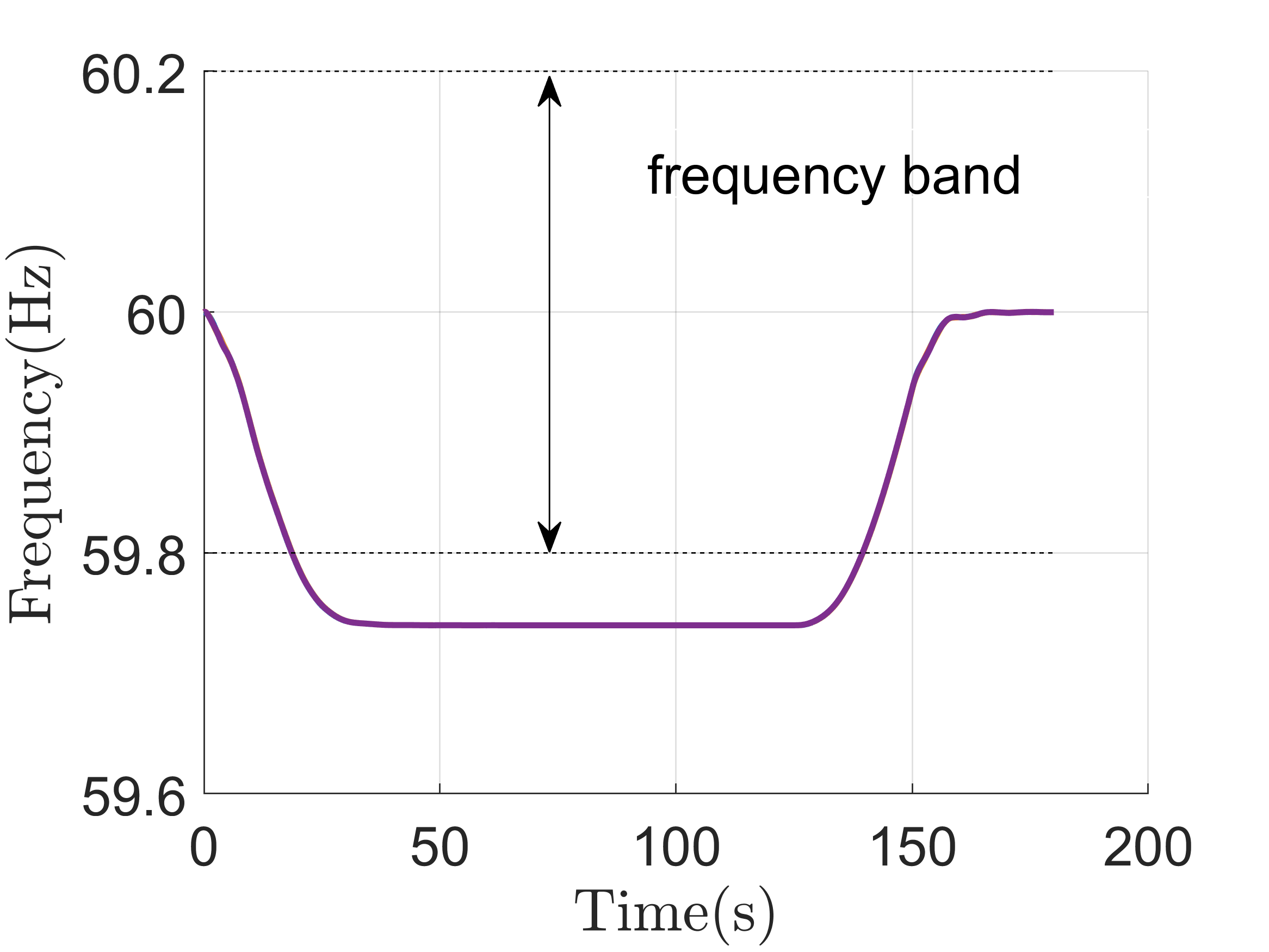
(a)

(b)

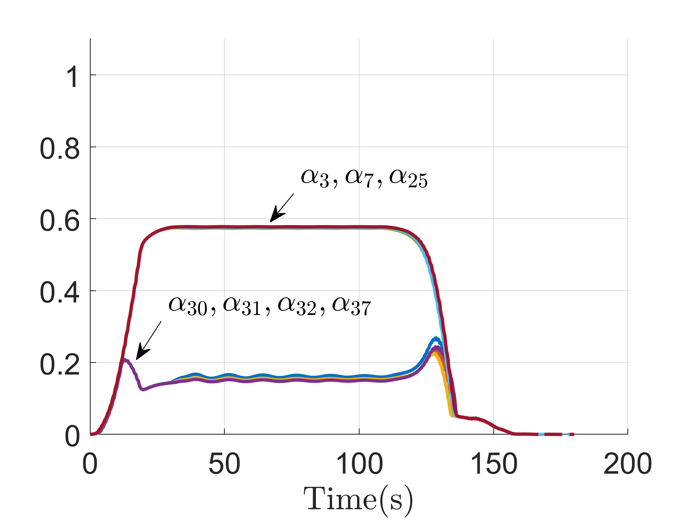
(c)

Figure 3: Frequency and control input trajectories with and without transient frequency control. Plot 3(a) shows the open-loop frequency responses at nodes 30, 31, 32, and 37, all exceeding the lower safe bound. The closed-loop system with the distributed control has all responses stay inside the safe region in plot 3(b). Plot 3(c) shows the corresponding control trajectories.

Next we compare the performance of the proposed controller with other approaches. Figures 44(a) and 4(b) show the frequency trajectories and control signals using the controller with regional coordination based on network decomposition proposed in [1]. As mentioned in Remark V.4, although this controller achieves frequency safety, it only allows control cooperation within a limited region, instead of the entire network. This can be seen from Figure 44(b), where, with the same control cost coefficients (cf. Table I), the two groups of control trajectories are not as uniform as those in Figure 33(c) and have a larger magnitude. Figures 44(c) and 4(d) are the frequency and control trajectories with only the top-layer controller, as proposed in [13], cf. Remark IV.9. Since it is a non-optimization-based control strategy, each control signal does not cooperate with others. In this specific scenario, the top-layer controller leads to fluctuations even during the time interval [25,125]$s$, when the disturbance is constant. This is because the top-layer controller is myopic, without further consideration for the effects of the rest of the network. The economic advantage of the proposed bilayered control can be also seen by computing the overall control cost over [0,180]$s$ of the proposed controller, the controller in [1], and the controller in [13], which are around 163, 231 and 656, resp.

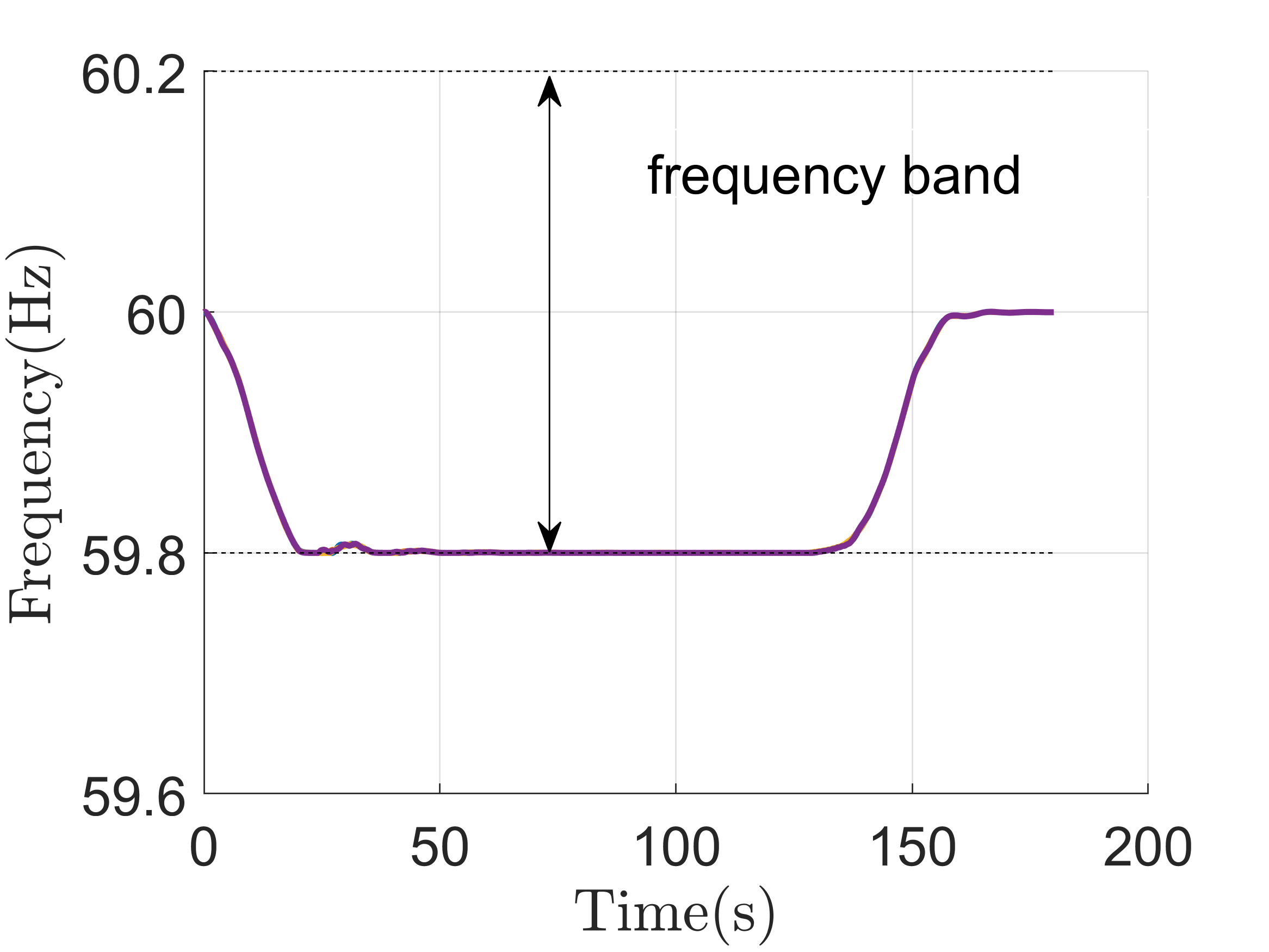
(a)

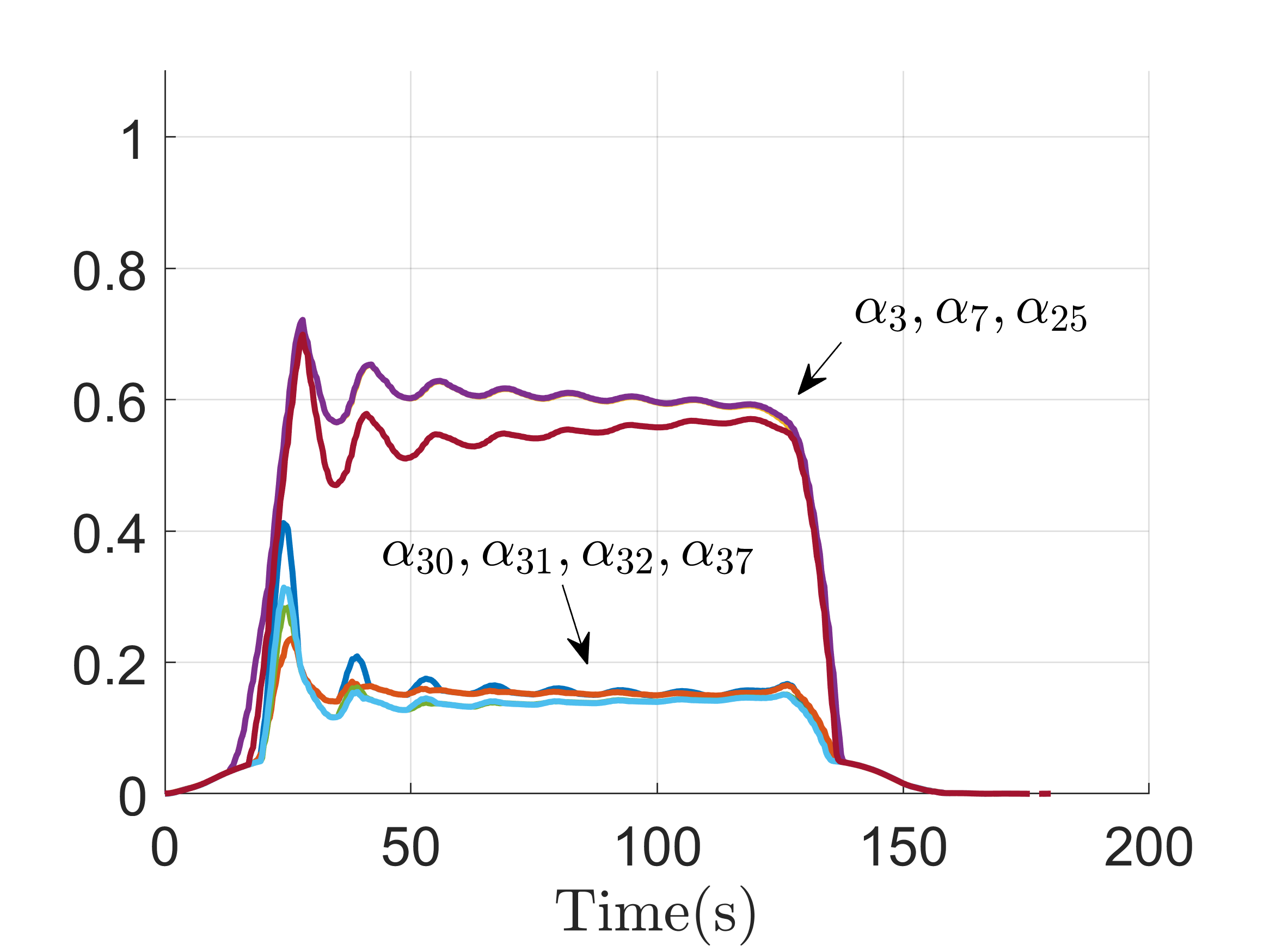
(b)

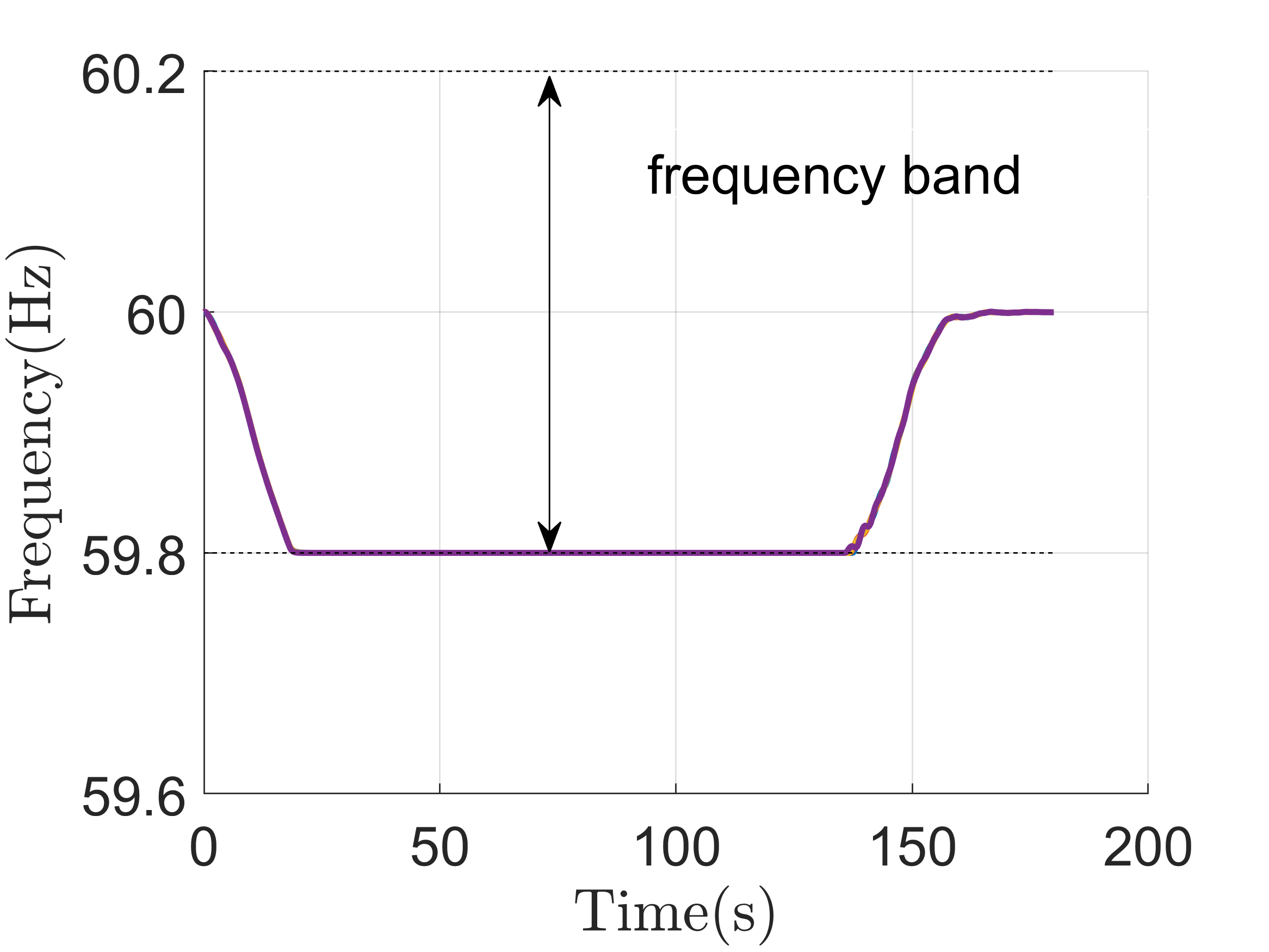
(c)

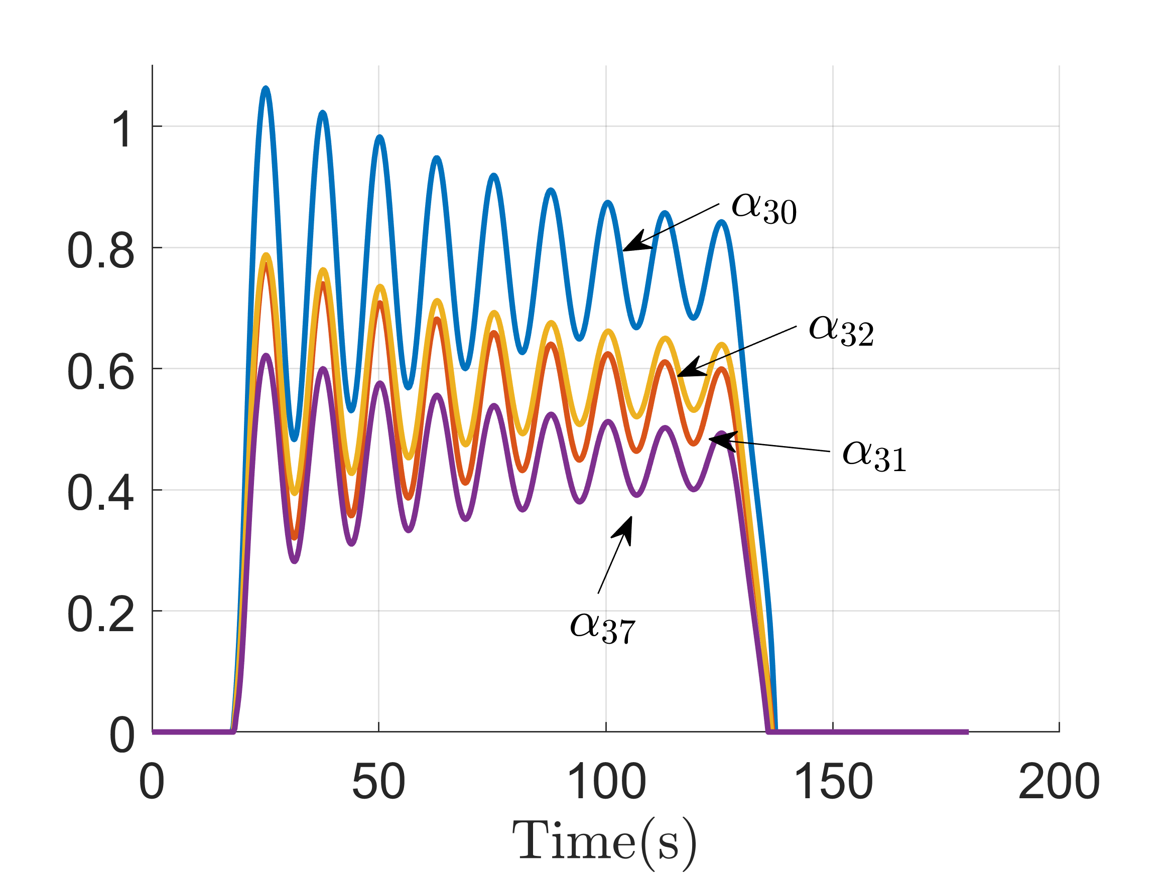
(d)

Figure 4: Comparison of frequency and control trajectories with other approaches. Plot 4(a) and 4(b) employ the controller with regional coordination based on network decomposition proposed in [1]. Plot 4(c) and 4(d) correspond to the top-layer controller, a non-optimization-based control strategy proposed in [13].

Next, we examine the role of the bottom and top layers in determining the value of the input signal of our distributed controller. For node $30$, Figure 55(a) shows that $\alpha_{BL,30}$ is responsible for the larger share in the overall control signal $\alpha_{30}$, whereas $\alpha_{TL,30}$ provides a slightly tuning during most of the time. If we reduce the penalty $d_{30}$ from 100 to 10, in Figure 55(b), the dominance of $\alpha_{BL,30}$ decreases, in accordance with our discussion in Remark IV.1. On the contrary, if we raise $d_{30}$ to 1000, the contribution of the top layer becomes much smaller, as shown in Figure 55(c).

We further look into the bottom-layer control signals at node 30. Using the same set-up as in Figure 55(a), we plot in Figure 66(a) the MPC component output signal $u_{MPC,30}$ and the stability filter output signal $\hat{u}_{MPC,30}$. They are almost identical except for a paltry difference around 140s. Next, in Figure 66(b), we purposefully add 0.1 to $u_{MPC,30}$, i.e., the input of the stability filter is now re-defined as $u_{MPC,30}+0.1$. Notice that $\hat{u}_{MPC,30}$, unaffected by the input shift, still converges to 0, which coincides with our analysis after Theorem IV.6. Figure 66(c) shows how the saddle-point dynamics (30) converges to the value of $u_{MPC,30}(50)$ starting from an initial guess. Here we have used $\epsilon_{Z}=5\cdot 10^{-4}$ and $\epsilon_{\eta}=\epsilon_{\mu}=2.5\cdot 10^{-4}$ to ensure convergence is attained within 1$s$, cf. Table I.

To illustrate the closed-loop system performance under uncertainty, in Figure 7 we simulate three different scenarios. In Figure 7(a), instead of having an accurate forecasted power injection, at every $t\geqslant 0$, we let $p^{fcst}_{t}(\tau)=p(t)$ for all $\tau\in[t,t+\tilde{t}]$, i.e., the forecasted power injection is simply the current power injection. Note that in this case the frequencies of all four controlled nodes stay within the safe region, cf. Remark IV.7; in Figure 7(b), for each generator node (i.e., node 30 to 39), we adopt a first-order model [32] with a time constant of $5s$ as the generator dynamics, and note that the frequencies still stay within the safe region most of the time; in Figure 7(c), we consider both inaccurate forecasted power injection and the generator dynamics, and the frequencies still behave well after a short fluctuation.

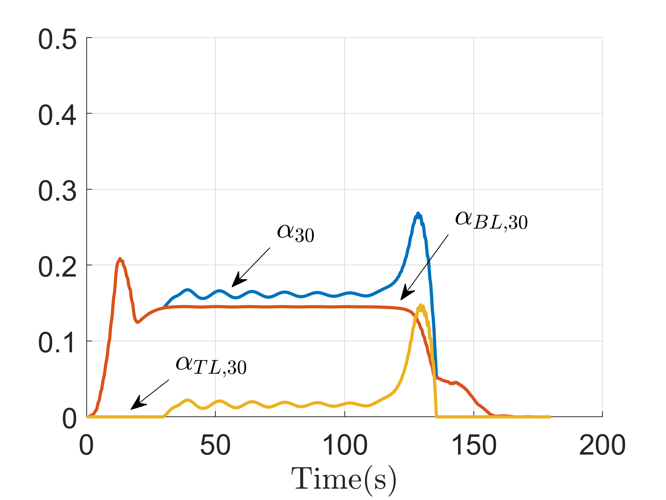
(a)

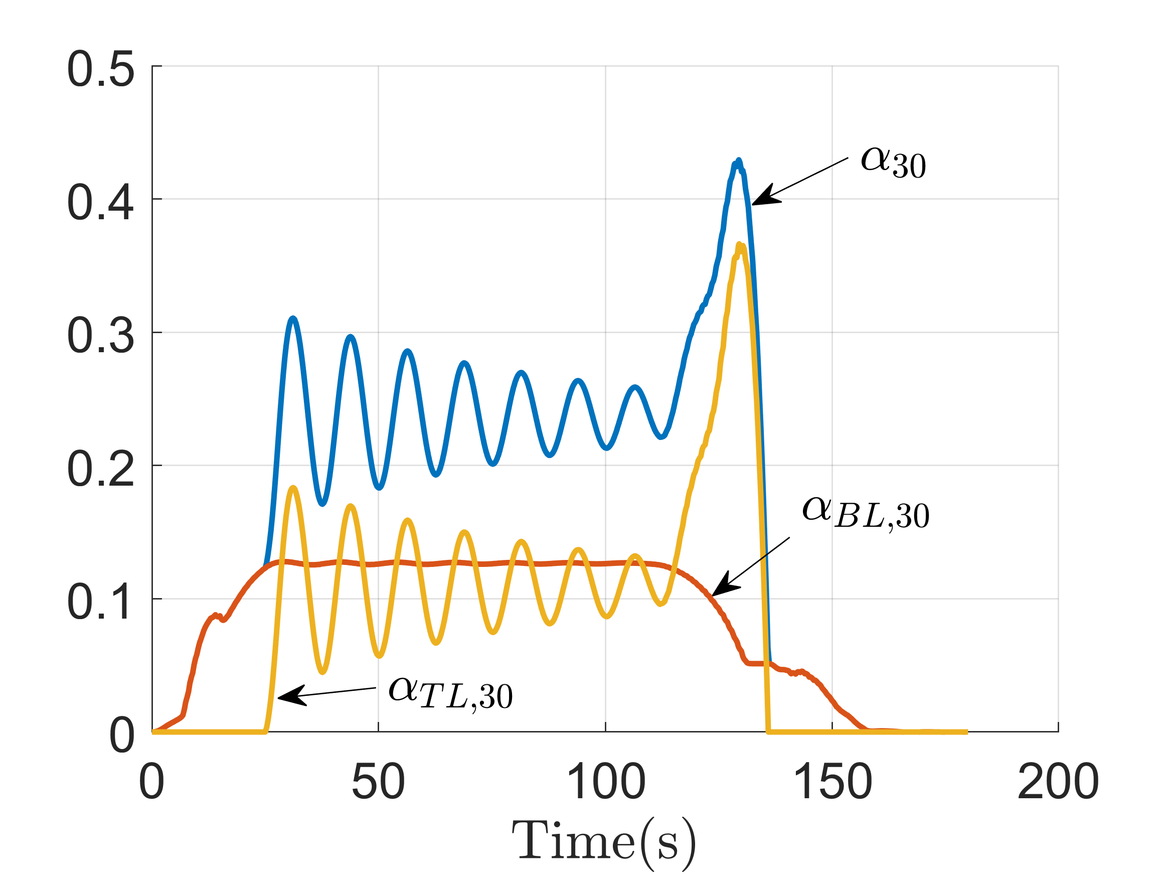
(b)

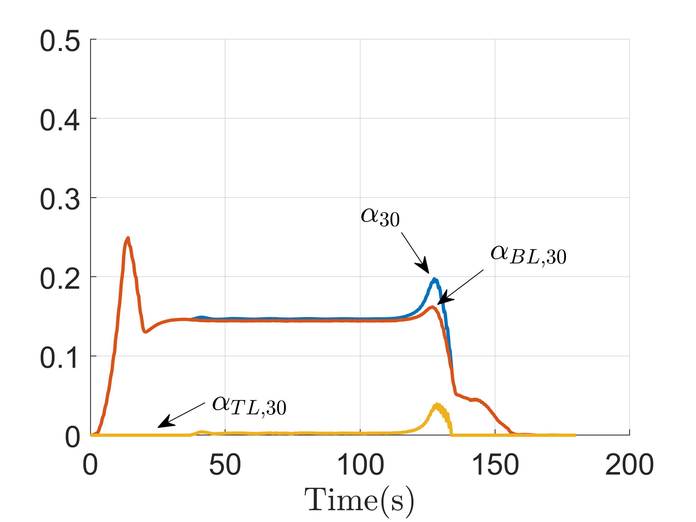
(c)

Figure 5: Decomposition of the control signal at node 30. Plot 5(a), 5(b), and 5(c) show the signals generated by the two control layers at node $30$ using $d_{30}=10^{2}$, $d_{30}=10$, and $d_{30}=10^{3}$, respectively, as values for the frequency safety violation penalty coefficient in the MPC component. With a larger penalty, the bottom layer plays a more significant role in the overall control signal.

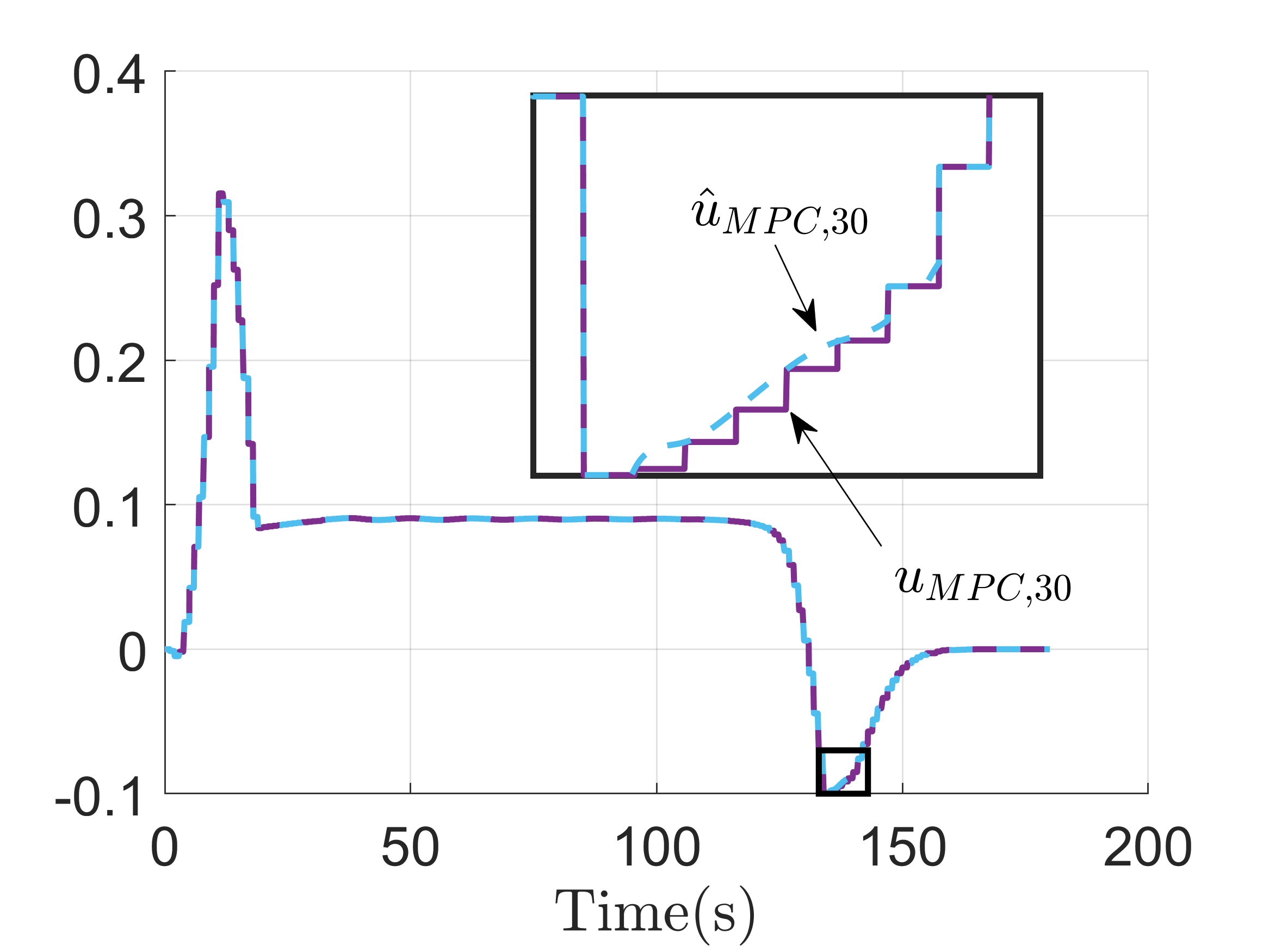
(a)

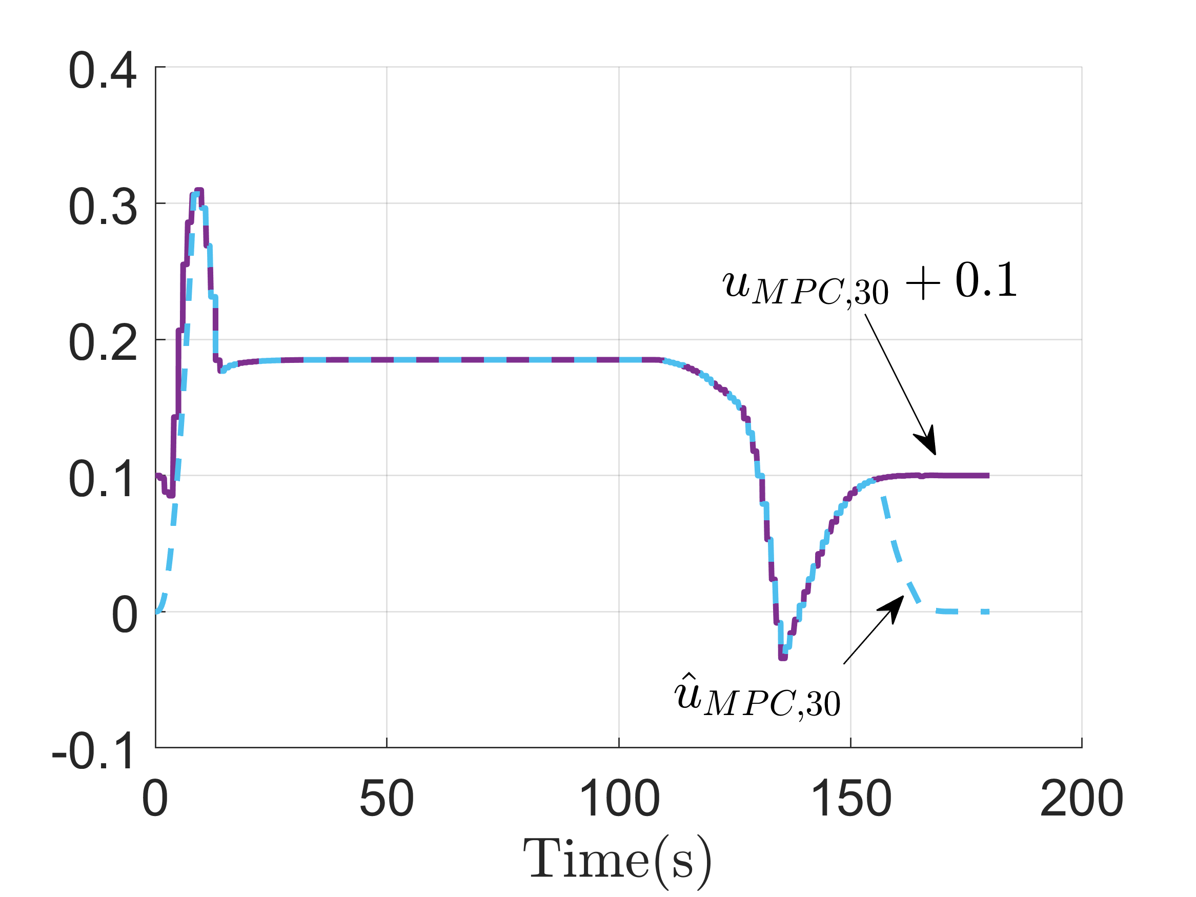
(b)

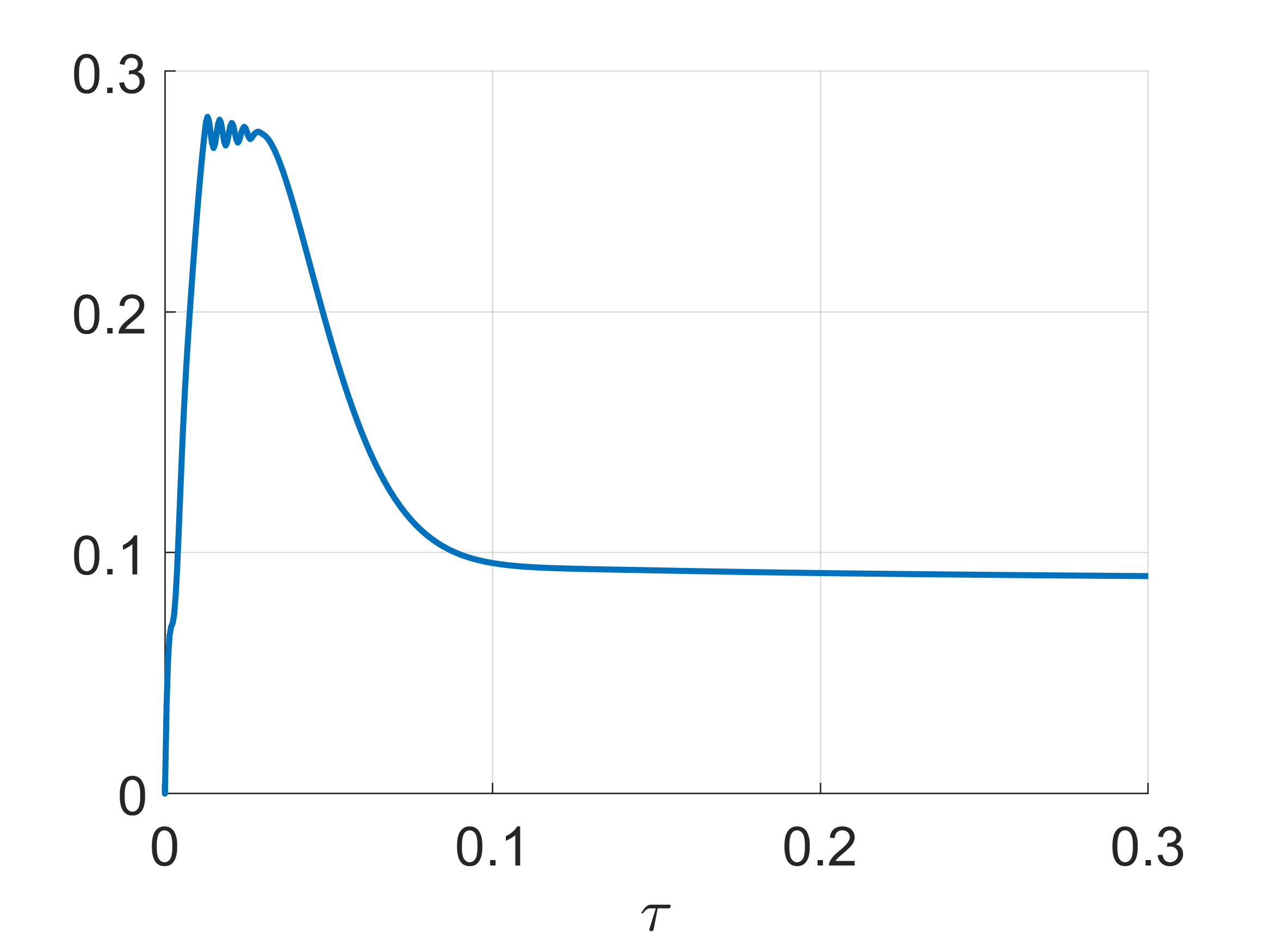
(c)

Figure 6: Decomposition of the bottom-layer control signal at node 30. Plot 6(a) shows the MPC component output signal $u_{MPC,30}$ and the stability filter output signal $\hat{u}_{MPC,30}$. Both are almost identical except for a minor discrepancy appearing around 140s. To make their difference more prominent, in plot 6(b), we add a constant 0.1 shift to $u_{MPC,30}$, which does not affect the convergence of $\hat{u}_{MPC,30}$ to 0 (highlighting again the fact that the MPC component cannot jeopardize system closed- loop asymptotic stability, cf. Remark IV.4). Plot 6(c) shows the convergence of the saddle-point dynamics (30) computing $u_{MPC,30}(50)$ in $0.1$s.

Lastly, we show that the distributed controller is able to steer the frequency to the safe region from unsafe initial conditions. To do this, we consider the set-up of Figure 3 but intentionally disable the controller for the first 30 seconds. For clarity, we only show the frequency and control trajectories at node 30 in Figure 8(a). Note that the frequency quickly moves above the safe lower bound after the controller becomes active at $t=30$s. Figure 8(b) shows the control signal, where after some brief transient, $\alpha_{BL,30}$ still dominates the overall control signal.

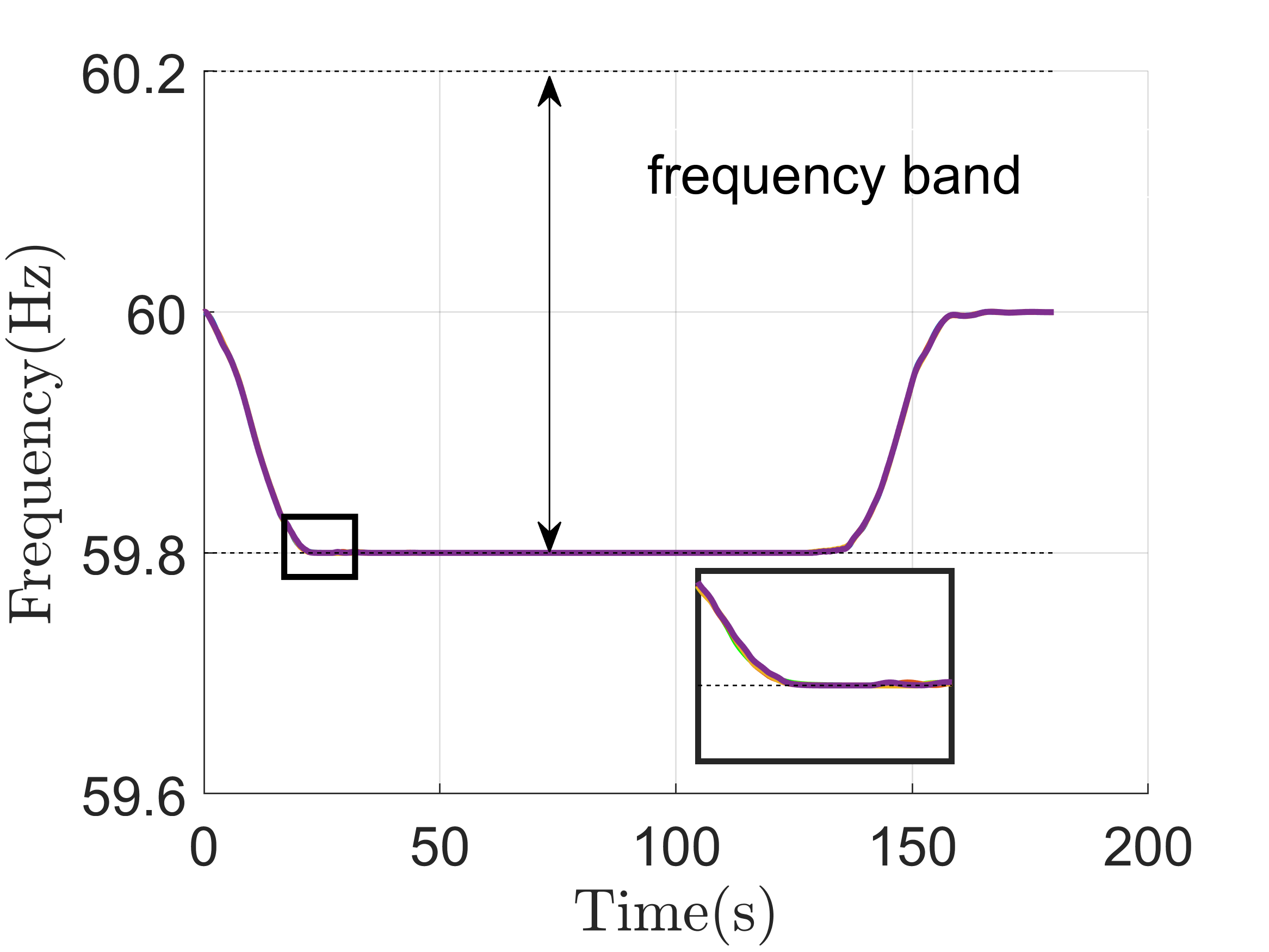
(a)

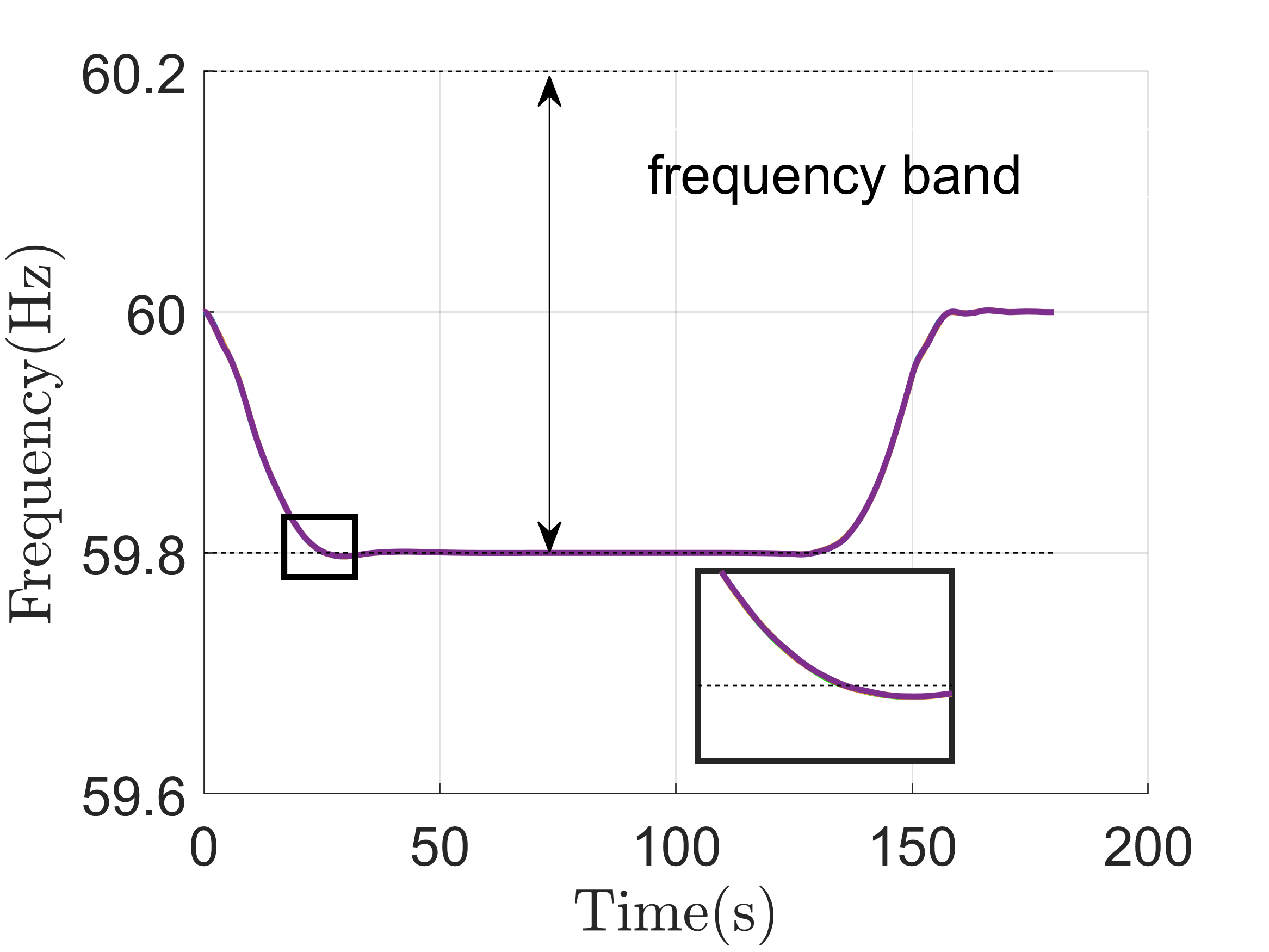
(b)

(c)

Figure 7: Frequency responses under inaccurate information and unmodeled dynamics. Plot 7(a), 7(b), and 7(c) show the frequency responses at nodes 30, 31, 32, and 37 under inaccurate forecasted power injection, first-order generator dynamics, and both, respectively.

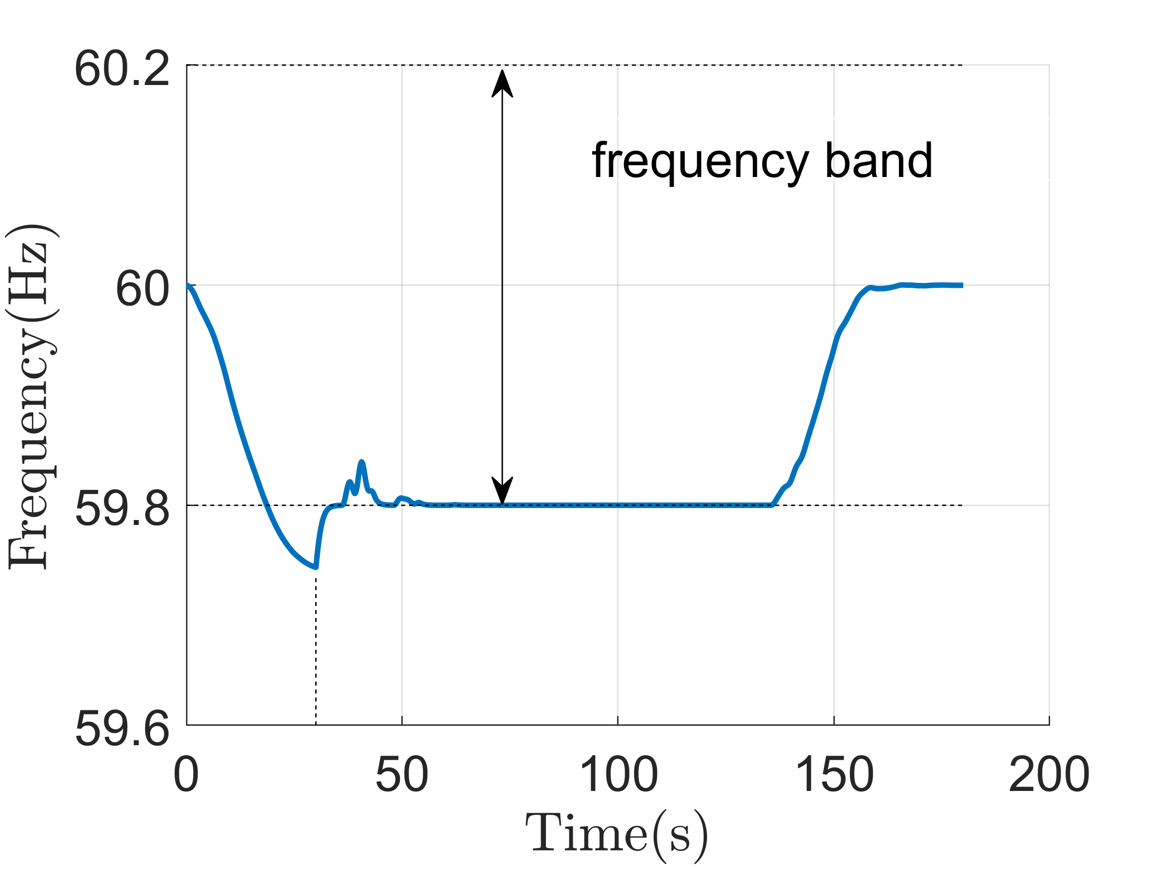
(a)

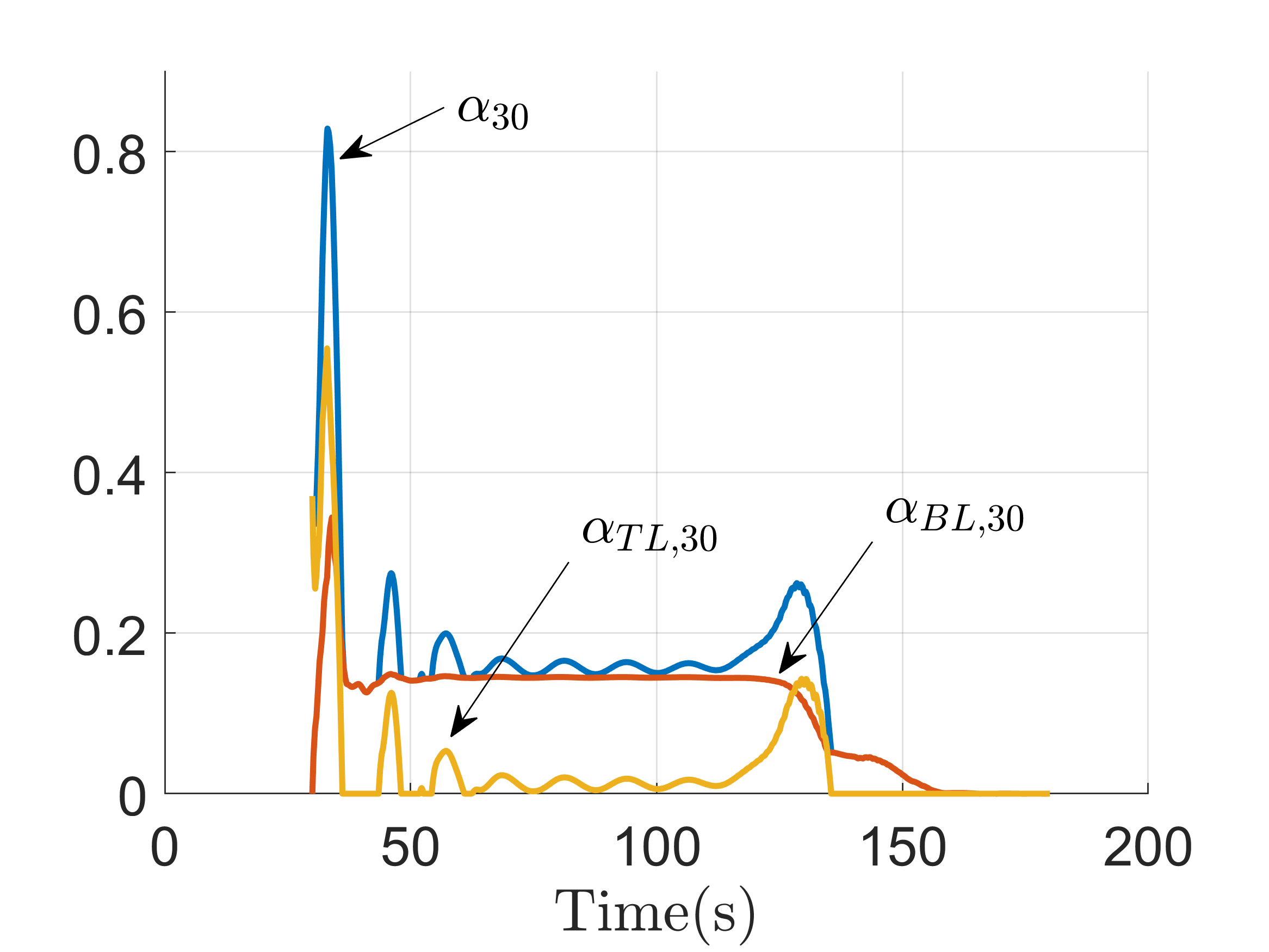
(b)

Figure 8: Frequency and control trajectories at node 30 when the controller is turned on after $30$s. In plot 8(a), the frequency gradually returns to the safe region once the controller kicks in. Plot 8(b) shows the control signals.

VII Conclusions

We have considered power networks governed by swing nonlinear dynamics and introduced a bilayered control strategy to regulate transient frequency in the presence of disturbances while maintaining network stability. Adopting a receding horizon approach, the bottom-layer controller periodically updates its output, enabling global cooperation among buses to reduce the overall control effort while respecting stability and soft frequency constraints. The top-layer controller, as a continuous state feedback controller, tunes the output of the bottom-layer control signal as required to rigorously enforces frequency safety and attractivity. We have shown that the entire control structure can be implemented in a distributed fashion, where the control signal can be computed by having nodes interact with up to 2-hop neighbors in the power network. Future work will explore the optimization of the sampling sequences employed in the bottom layer to improve performance, the quantitative evaluation of the contributions of the top- and bottom-layer control signals, and the analysis of the robustness of the proposed controller against delays and saturation.

Yifu Zhang received the B.S. degree in automatic control from the Harbin Institute of Technology, Heilongjiang, China, in 2014, and the Ph.D. degree in mechanical engineering from the University of California, San Diego, CA, USA, in 2019. In winter 2019, he interned at Mitsubishi Electric Research Laboratories, MA, USA. Currently he is a senior software quality engineer at The MathWorks, Inc., MA, USA. His research interests include distributed control and computation, model predictive control, adaptive control, data type optimization, function approximation, and neural network compression.

Jorge Cortés (M’02, SM’06, F’14) received the Licenciatura degree in mathematics from Universidad de Zaragoza, Zaragoza, Spain, in 1997, and the Ph.D. degree in engineering mathematics from Universidad Carlos III de Madrid, Madrid, Spain, in 2001. He held postdoctoral positions with the University of Twente, Twente, The Netherlands, and the University of Illinois at Urbana-Champaign, Urbana, IL, USA. He was an Assistant Professor with the Department of Applied Mathematics and Statistics, University of California, Santa Cruz, CA, USA, from 2004 to 2007. He is now a Professor in the Department of Mechanical and Aerospace Engineering, University of California, San Diego, CA, USA. He is the author of Geometric, Control and Numerical Aspects of Nonholonomic Systems (Springer-Verlag, 2002) and co-author (together with F. Bullo and S. Martínez) of Distributed Control of Robotic Networks (Princeton University Press, 2009). At the IEEE Control Systems Society, he has been a Distinguished Lecturer (2010-2014) and is currently its Director of Operations and an elected member (2018-2020) of its Board of Governors. His research interests include distributed control and optimization, network science, resource-aware control, nonsmooth analysis, reasoning and decision making under uncertainty, network neuroscience, and multi-agent coordination in robotic, power, and transportation networks.

References

- [1] Y. Zhang and J. Cortés, “Double-layered distributed transient frequency control with regional coordination,” in American Control Conference, Philadelphia, PA, Jul. 2019, pp. 658–663.
- [2] P. Kundur, J. Paserba, V. Ajjarapu, G. Andersson, A. Bose, C. Canizares, N. Hatziargyriou, D. Hill, A. Stankovic, C. Taylor, T. V. Cutsem, and V. Vittal, “Definition and classification of power system stability,” IEEE Transactions on Power Systems, vol. 19, no. 2, pp. 1387–1401, 2004.
- [3] NERC, “Balancing and frequency control,” North American Electric Reliability Council, Tech. Rep., 2011.
- [4] F. Milano, F. Dörfler, G. Hug, D. J. Hill, and G. Verbič, “Foundations and challenges of low-inertia systems,” in Power Systems Computation Conference, Dublin, Ireland, June 2018, electronic proceedings.
- [5] F. Dörfler, M. Chertkov, and F. Bullo, “Synchronization in complex oscillator networks and smart grids,” Proceedings of the National Academy of Sciences, vol. 110, no. 6, pp. 2005–2010, 2013.
- [6] H. D. Chiang, Direct Methods for Stability Analysis of Electric Power Systems: Theoretical Foundation, BCU Methodologies, and Applications. John Wiley and Sons, 2011.
- [7] T. L. Vu, H. D. Nguyen, A. Megretski, J. Slotine, and K. Turitsyn, “Inverse stability problem and applications to renewables integration,” IEEE Control Systems Letters, vol. 2, no. 1, pp. 133–138, 2018.
- [8] J. Fang, H. Li, Y. Tang, and F. Blaabjerg, “Distributed power system virtual inertia implemented by grid-connected power converters,” IEEE Transactions on Power Electronics, vol. 33, no. 10, pp. 8488–8499, 2018.
- [9] S. S. Guggilam, C. Zhao, E. Dall’Anese, Y. C. Chen, and S. V. Dhople, “Optimizing DER participation in inertial and primary-frequency response,” IEEE Transactions on Power Systems, vol. 33, no. 5, pp. 5194–5205, 2018.
- [10] F. Teng, M. Aunedi, D. Pudjianto, and G. Strbac, “Benefits of demand-side response in providing frequency response service in the future GB power system,” Frontiers in Energy Research, vol. 3, no. 36, 2015.
- [11] A. D. Ames, S. Coogan, M. Egerstedt, G. Notomista, K. Sreenath, and P. Tabuada, “Control barrier functions: theory and applications,” in European Control Conference, Naples, Italy, Jun. 2019, pp. 3420–3431.
- [12] H. K. Khalil, Nonlinear Systems, 3rd ed. Prentice Hall, 2002.
- [13] Y. Zhang and J. Cortés, “Distributed transient frequency control for power networks with stability and performance guarantees,” Automatica, vol. 105, pp. 274–285, 2019.
- [14] ——, “Model predictive control for transient frequency regulation of power networks,” Automatica, 2020, submitted.
- [15] H. Jiang, J. Lin, Y. Song, and D. J. Hill, “MPC-based frequency control with demand-side participation: A case study in an isolated wind-aluminum power system,” IEEE Transactions on Power Systems, vol. 30, no. 6, pp. 3327–3337, 2015.
- [16] A. N. Venkat, I. A. Hiskens, J. B. Rawlings, and S. J. Wright, “Distributed MPC strategies with application to power system automatic generation control,” IEEE Transactions on Control Systems Technology, vol. 16, no. 6, pp. 1192–1206, 2008.
- [17] A. Fuchs, M. Imhof, T. Demiray, and M. Morari, “Stabilization of large power systems using VSC-HVDC and model predictive control,” IEEE Transactions on Power Delivery, vol. 29, no. 1, pp. 480 – 488, 2014.
- [18] F. Bullo, J. Cortés, and S. Martinez, Distributed Control of Robotic Networks, ser. Applied Mathematics Series. Princeton University Press, 2009.
- [19] A. R. Bergen and D. J. Hill, “A structure preserving model for power system stability analysis,” IEEE Transactions on Power Apparatus and Systems, vol. 100, no. 1, pp. 25–35, 1981.
- [20] A. Pai, Energy Function Analysis for Power System Stability. New York: Springer, 1989.
- [21] F. Borrelli, Constrained Optimal Control of Linear and Hybrid Systems. New York: Springer, 2003.
- [22] A. Alessio and B. Alberto, “A survey on explicit model predictive control,” in Nonlinear Model Predictive Control. Springer, 2009, pp. 345–369.
- [23] S. Boyd and L. Vandenberghe, Convex Optimization. Cambridge University Press, 2004.
- [24] A. Cherukuri, E. Mallada, S. H. Low, and J. Cortés, “The role of convexity in saddle-point dynamics: Lyapunov function and robustness,” IEEE Transactions on Automatic Control, vol. 63, no. 8, pp. 2449–2464, 2018.
- [25] E. Mallada, C. Zhao, and S. H. Low, “Optimal load-side control for frequency regulation in smart grids,” IEEE Transactions on Automatic Control, vol. 62, no. 12, pp. 6294–6309, 2017.
- [26] M. H. Nazari, Z. Costello, M. J. Feizollahi, S. Grijalva, and M. Egerstedt, “Distributed frequency control of prosumer-based electric energy systems,” IEEE Transactions on Power Systems, vol. 29, pp. 2934–2942, 2014.
- [27] P. Trodden and A. Richards, “Cooperative distributed MPC of linear systems with coupled constraints,” Automatica, vol. 49, no. 2, pp. 479–487, 2013.
- [28] P. Giselsson, M. D. Doanb, T. Keviczky, B. D. Schutter, and A. Rantzer, “Accelerated gradient methods and dual decomposition in distributed model predictive control,” Automatica, vol. 49, no. 3, pp. 829–833, 2013.
- [29] X. Wang, S. Mou, and B. D. O. Anderson, “Scalable, distributed algorithms for solving linear equations via double-layered networks,” IEEE Transactions on Automatic Control, 2020, to appear.
- [30] M. Zhu and S. Martínez, “On distributed convex optimization under inequality and equality constraints,” IEEE Transactions on Automatic Control, vol. 57, no. 1, pp. 151–164, 2012.
- [31] K. W. Cheung, J. Chow, and G. Rogers, Power System Toolbox, v 3.0. Rensselaer Polytechnic Institute and Cherry Tree Scientific Software, 2009.
- [32] Z. Wang, F. Liu, S. H. Low, C. Zhao, and S. Mei, “Distributed frequency control with operational constraints, part I: Per-node power balance,” IEEE Transactions on Smart Grid, vol. 9, no. 4, pp. 1798–1811, 2018.