CO Detected in CI Tau b: Hot Start Implied by Planet Mass and M_K

Abstract

We acquired high resolution IR spectra of CI Tau, the host star of one of the few young planet candidates amenable to direct spectroscopic detection. We confirm the planet’s existence with a direct detection of CO in the planet’s atmosphere. We also calculate a mass of 11.6 M_J based on the amplitude of its radial velocity variations. We estimate its flux contrast with its host star to get an absolute magnitude estimate for the planet of 8.17 in the K band. This magnitude implies the planet formed via a “hot start” formation mechanism. This makes CI Tau b the youngest confirmed exoplanet as well as the first exoplanet around a T Tauri star with a directly determined, model-independent, dynamical mass.

1 Introduction

Observations of young exoplanets are key to understanding planet formation. Models for giant planets indicate planets can form with very different temperatures at early ages. It is often assumed that gravitational instability produces hot planets while core accretion forms comparatively cooler and less luminous planets (Marley et al., 2007b), although it may be possible for both formation models to produce planets at a range of temperatures (Helled et al., 2014). To better distinguish between these possibilities, young planets with model-independent masses are needed. Several planets have been found via direct imaging around pre-main sequence stars, including some around T Tauri stars (e.g., Chauvin et al., 2004; Ireland et al., 2011; Rameau et al., 2013), and their measured magnitudes have been used to evaluate planet formation theories (Marleau & Cumming, 2014; Rajan et al., 2017). However, for these systems, the planet mass estimates are necessarily model-dependent as it is generally not possible to detect the stellar reflex motion given the extreme mass ratios and the large star-companion separations. With the exception of $\beta$ Pic b (Snellen & Brown, 2018; Dupuy et al., 2019), confirmation of these objects as planetary mass companions is not yet possible.

Young stars are significantly more active than main sequence stars, which hides the subtle planetary signals, making detection via either the radial velocity (RV) or the transit method difficult. However, in the past several years, planet candidates have been reported around pre-main sequences stars using the RV method including CI Tau b (Johns-Krull et al., 2016), V830 Tau b (Donati et al., 2016), and Tap 26 b (Yu et al., 2017). These targets would be ideal for evaluating planetary evolution models if the planet’s brightness or temperature could be determined. To do so, the planet needs to be detectable directly. By virtue of being close enough to their host stars to induce substantial gravitational reflex motion, these planets are too close to be detected via direct imaging.

Direct spectroscopic detection has been used to measure both planet masses and contrast ratios between absorption lines in hot Jupiter atmospheres and their main sequence host stars’ continuum (e.g. Snellen et al., 2010; Brogi et al., 2012; Birkby et al., 2013; Rodler et al., 2013). Near infrared spectra are used to detect molecules common in planetary atmospheres like H₂O and CO. By using spectra from different phases in the planet’s orbit, the median stellar signal can be simply subtracted out, while the planet’s signal, which is moving at hundreds of kilometers per second, remains, allowing for a direct detection of the planet’s spectrum.

CI Tau is a $\sim$2-3 Myr old, K7, classical T Tauri star. Johns-Krull et al. (2016) detected a M_Psini=8.08$\pm$1.53 M_J planet candidate around it with a 8.989 day period based on analysis of its RV variations. Based on an inclination of $\sim 44^{\circ}$ estimated from imaging its disk (Guilloteau et al., 2014), its total mass is $\sim$11 M_J. If the planet formed via some “hot start” mechanism, its expected contrast ratio with its host star should be a few$\times$10^-3 based on models from Spiegel & Burrows (2012) and thus would be directly detectable spectroscopically. If, however, the planet formed via a “cold start” method, its contrast ratio would likely be $\sim 10^{-5}$ at best, a ratio no current techniques are sensitive to.

2 Observations and Data Analysis

2.1 Observations

Our 40 observations of CI Tau were taken between 2014-2018 with the Immersion Grating Infrared Spectrograph (IGRINS) at both the McDonald Observatory 2.7-m Harlan J. Smith Telescope and the Lowell Observatory 4.3-m Discovery Channel Telescope. CI Tau was observed by nodding between the A and B positions on the slit. Total exposure times ranged from 240 to 2400 seconds, resulting in final S/N values of 125-300. Each target observation was paired with a standard A0V star observation at a similar airmass used for telluric corrections. IGRINS makes use of a silicon immersion grating and a fixed optical path to simultaneously cover the H and K bands (1.45-2.5$\mu$m) with a spectral resolving power R$\sim$45,000. Additional discussion on the design and capabilities of IGRINS can be found in Park et al. (2014); Mace et al. (2018).

2.2 Data Reduction

We reduced the data with the IGRINS pipeline package (version 2.2.0 alpha 1; Lee et al., 2017). The pipeline implements flat-fielding, bad pixel correction, sky subtraction, and source extraction based on the methods of Horne (1986). The pipeline wavelength solution is based on telluric emission and absorption lines.

To continuum normalize, we fit a 6th order polynomial to each order of the spectrum of an A0V star taken the same night. We scale this fit to account for differences in the maximum flux, and then divide each CI Tau spectrum by the scaled fit to remove the blaze function. Because it is critical to have all observations on the same wavelength scale, we then cross-correlate the 2.06 - 2.08 $\mu m$ order with a telluric template. At these wavelengths, the spectrum is dominated by telluric features. We corrected for any discrepancies by shifting the wavelength solution for the all CI Tau spectral orders by the offset between the telluric lines in the target and in the A0V spectrum. All spectra are then interpolated onto a common wavelength scale with a spacing of 2.04 km/s per pixel to match the native resolution of IGRINS.

2.3 Removing Telluric and Stellar Features

We used spectra of A0V stars to correct for the telluric features. As the telluric spectra were generally not taken at the exact same airmass as the target, we raised the flux of the continuum normalized telluric spectrum to a power to account for changes in line strength. This power was determined by fitting each A0V spectra using the Levenberg-Marquardt algorithm to perform a least-squares minimization (Newville et al., 2014) until the telluric lines in the A0V star matched the depth of the telluric lines in the target spectra. We do not currently adjust for compositional differences in the telluric spectra, so we use A0V spectra taken close in time to the target spectra. Our method for removing telluric features worked relatively well in regions where there is not too much telluric absorption. However, there are regions of the spectrum that correct poorly with this method because of very strong telluric absorption. We chose to mask those regions out of the analysis. After telluric correction, we then corrected each CI Tau spectrum for barycentric velocity differences.

CI Tau has a protoplanetary disk, therefore we also need to correct for differences in the CI Tau spectra due to continuum veiling, the ratio of the excess disk flux to the flux from the stellar continuum. We took the observation with the least amount of veiling and de-veil all other observations to match that one. We estimated the overall veiling of this least veiled CI Tau spectrum by fitting it to a template spectrum accounting for differences in rotational broadening, following Johns-Krull & Valenti (2001). For the template, we use IGRINS spectra of V830 Tau, a diskless star of the same age and spectral type. While Donati et al. (2016) report that V830 Tau has a planet, the strength of any lines contributed by the planet is expected to make a negligible change in the derived veiling.

After correcting each observation for telluric absorption and veiling, the stellar spectrum ideally should not change except for the signal of the planet moving in velocity space. To ensure we have removed as much of the star’s signal as possible, we needed to correct for any slight differences in velocity. We cross-correlated each stellar spectrum with the highest signal to noise spectrum, so that we could Doppler shift them to the same stellar frame. We then subtracted the median spectrum, ideally leaving only the planet’s signal, and shifted the spectra back to their original frame. T Tauri stars’ variability arises from other processes in addition to veiling. As a result, it is difficult to account for all variability in the target spectra even after subtracting the median (see section 3).

2.4 Planet Detection via Cross-Correlation

We employ two methods to magnify the weak signal from the planet. One is by phase shifting the spectra so the planet’s signal from observations at different phases of the planet’s orbit, initially at different of RVs, is aligned; we then co-added all the spectra. The other is cross-correlating the spectrum with a template which combines the signal from all the spectral features into one signal. We chose to base our analysis by first co-adding and then cross-correlating; however, reversing the order also results in a detection as described below.

In order to shift the spectra to account for the planet’s orbital motion, its orbit must already be known. We fixed the orbital parameters at the values listed in Table 1 from Johns-Krull et al. (2016). However, the stellar inclination is not derived from the RV curve. The velocity amplitude of the star could be caused by a more massive planet on a more face-on orbit or a less massive planet on a more edge-on orbit. This also impacts the RV shift of the planet with a larger planetary velocity amplitude, K_P, occurring if the orbit is more edge on. As we cannot assume a K_P from the stellar RV curve, we vary K_P in increments of 1 km/s over the region of physically allowable parameter space to look for the strongest signal. For each value of K_P, we calculate the cross-correlation function at a range of offsets between -400 and 400 km/s in increments corresponding to the velocity spacing of the pixels. The template for the cross-correlation is created from VALD (Ryabchikova et al., 2015), which used the CO line list from Kurucz (2010), for an object of T_eff=2500 K with logg=4.0 dex. Because of the reliance on the CO lines for the reported detection, we used only 4 orders of the spectra that covered wavelengths between 2.29 and 2.42 $\mu m$.

3 Results

The cross-correlation matrix (Figure 1) peaks at at a systemic RV, V_sys=18.0$\pm_{4.4}^{3.7}$ km/s and K_P=77.4$\pm_{9.4}^{7.0}$ km/s. The value of V_sys is consistent within uncertainties to that measured by Torres et al. (2006). To estimate the significance of this detection, we adapted the method from Birkby et al. (2013). We took the CCF matrix, subtracted the mean CCF value and divided by the standard deviation of the values away from the signal as in Hoeijmakers et al. (2018). Using this, the peak has a significance of 5.7$\sigma$. If we first cross-correlate each individual CI Tau spectrum with the template and then sum the cross correlation functions, the peak occurs at V_sys = 17.1 km/s and K_P = 77.9 km/s (both equal to within the uncertainties to the values above) with a significance of 4.8$\sigma$. We also detect the signal in each of the four orders and each observing season separately. The 1$\sigma$ uncertainty in K_P and V_sys is taken as the points in the CCF matrix where the CCF value has dropped by 1, i.e from 5.7 to 4.7, as in Brogi et al. (2018). To verify this uncertainty, we have created a bootstrap sample (Efron, 1979) of N=10000 data sets of 40 spectra, randomly sampling with replacement from our original 40 spectra. We then calculate V_sys and K_P for each of the N data sets, creating a new distribution with N values for each parameter. This resulted in measurements of V_sys=18.3$\pm_{1.8}^{2.7}$ km/s and K_P=76.9$\pm_{5.6}^{4.9}$ km/s, with the 1$\sigma$ error bars corresponding to the 68.3% confidence interval from these distributions. We chose to be conservative and use the larger uncertainties above for further analysis. Uncertainties in K_P and K_∗ dominate the uncertainties in the additional quantities derived below.

Table 1: Parameters of the CI Tau System

Parameter		Value
M∗ (M⊙)		0.90$\pm$0.02
K∗ (km/s)		0.950$\pm$0.207
distance (pc)		158.0$\pm$1.2
orbital period (days)		8.9891$\pm$0.0202
eccentricity		0.25$\pm$0.16
angle of periastron (∘)		31$\pm$56
KP (km/s)		77.4$\pm_{9.4}^{7.0}$
MP (MJ)		11.6$\pm_{2.7}^{2.9}$

Note. — Distance from Simon et al. (in prep), based on Gaia (Brown et al., 2018) and Bailer-Jones et al. (2018). Stellar mass, initially measured by Guilloteau et al. (2014) adjusted for distance and the planet’s mass.

Based on the determined value of K_P and the velocity amplitude of the star, K_∗, we calculated a mass ratio $\frac{M_{*}}{M_{P}}$ of 81.5$\pm_{20.3}^{19.2}$. We assume a stellar mass of 0.9 M_⊙. This leads to a planet mass of 11.6$\pm_{2.7}^{2.9}$ M_J. Our detection is fully consistent with planet parameters reported in Johns-Krull et al. (2016). Based on the mass of the planet and its separation with its host star, models indicate that it could not form at its current location (Dawson & Johnson, 2018, and sources therein). Thus, the planet likely formed elsewhere in the disk and then moved inward.

We have calculated an inclination of 50.5$\pm_{8.5}^{6.3}$ degrees, using sin(i)=$\frac{K_{P}}{V_{P}}$, where V_P is the orbital velocity amplitude calculated from Kepler’s Laws using the assumed stellar mass, eccentricity, and period. This is within uncertainties of disk inclinations previously measured, which are in the range of 44 to 51^∘ (Guilloteau et al., 2014; Tripathi et al., 2017; Clarke et al., 2018). Given these inclinations, we do not expect the planet to transit.

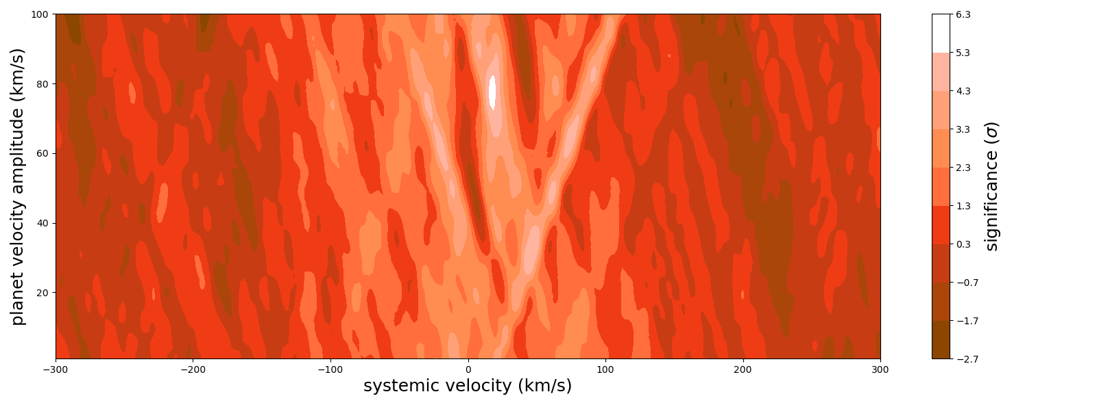
Figure 1: The cross-correlation function significance plotted as a function of planet velocity amplitude and systemic radial velocity. The significance is the number of standard deviations above the mean for those parameters, peaking at 5.7$\sigma$.

The cross-correlation plot (Figure 1) shows residuals that we believe come from the star itself. Unlike host stars that are typical targets for direct detection, CI Tau is a relatively cool star and thus has some of the same CO features we are attempting to detect in the planet. Given the star is young and variable, our method likely does not completely remove the star’s signal from the spectra. For example, the spot coverage on the star is expected to vary which should produce small differences in the CO spectra coming from the star. As a result, there are likely artifacts from the star that show up in Figure 1, specifically the v-shaped feature that starts from the lower axis of the plot at the systemic velocity of the star, which is likely due to CI Tau itself.

Of particular interest from this detection is the contrast ratio between the star and the planet. By inserting simulated planets at random systemic and orbital velocities, we can estimate the contrast ratio needed to produce the signal we see. Our best estimate for the flux ratio between the star+disk and planet is 356$\pm_{69}^{94}$. With our estimated veiling of 1.08$\pm$0.16 for the least veiled observation of CI Tau, (which is consistent with other veiling measurements for CI Tau - Sokal et al., submitted) this results in a star to planet flux ratio of 172$\pm_{37}^{54}$. Based on the contrast ratio between the planet and the star+disk, CI Tau’s apparent magnitude of 7.793 in the K band from 2MASS (Skrutskie et al., 2006), and the system’s distance, we calculate an absolute magnitude of 8.17$\pm_{0.21}^{0.33}$ in the K band for CI Tau b.

4 Discussion and Conclusions

We have analyzed K band spectra of CI Tau and found strong support of the existence of CI Tau b, a hot Jupiter with a mass of 11.6$\pm_{2.7}^{2.9}$ M_J. We have directly detected CO in CI Tau b’s atmosphere. We have also estimated its magnitude in the K band. These results make CI Tau b the youngest confirmed exoplanet and the only exoplanet around a T Tauri star with a model-independent mass.

Based on models of young, giant exoplanets (Spiegel & Burrows, 2012), a planet would need to form via a “hot start” mechanism to be this bright at a 10 M_J planetary mass. This confirms hot start models as a viable scenario for planet formation for the case of CI Tau b. In addition, according to Spiegel & Burrows (2012), a 10 M_J planet at 2 Myr would have a radius of $\sim$2 R_J and a T${}_{eff}\sim$2300 K; Baraffe et al. (2015) give similar numbers for a 0.01 M_⊙ (10.5 M_J) object at that age. This bright magnitude is consistent with other planetary mass companions around young stars, which also appear consistent with a hot start formation (Figure 2). However, other than $\beta$ Pic b and now CI Tau b, thus far none of those objects have model independent masses needed to confirm them as planets.

Even a cold-start planet can have a high surface temperature if its surface is externally heated. Assuming the planet is tidally locked, we can estimate its equilibrium temperature as $T_{eq}=\left(\frac{(1-A_{b})L_{S}}{8\pi\sigma d^{2}}\right)^{1/4}$, with L_∗ the host star’s total luminosity, $d$ the separation, $\sigma$ the Stefan-Boltzman constant, and $A_{b}$ the planet’s albedo (Marley et al., 2007a). We combined the intrinsic stellar luminosity of 0.6 L_⊙ (McClure et al., 2013a) with the accretion luminosity of 0.3 L_∗ (Valenti et al., 1993), for a total source luminosity of 0.78 L_⊙. Based on this, we calculated temperatures ranging from 820 to 1080 K, depending on the planet’s albedo. There also may be heating from the inner disk wall. McClure et al. (2013a) gives an inner wall luminosity of 0.08 L_∗. We estimated the flux from the disk that reaches the planet when at apastron by integrating the flux from the inner disk wall over its area, using the height and radius of the disk wall from McClure et al. (2013b). Adding this flux to the flux from the star and accretion luminosity results in temperatures between 1000 and 1300 K. Thus, it is unlikely that CI Tau b’s proximity to its host star or the disk is responsible for its bright K band magnitude.

Figure 2: Absolute K magnitude versus age for a selection of planetary mass companions. In red are the hot start tracks from Spiegel & Burrows (2012), while the cold start tracks are in blue. The known planetary mass companions around the youngest stars appear consistent with a hot start formation. Magnitudes for 2MASS J12073346-3932539, HD 95086 b, 1RXS J160929.1 − 210524 b, $\beta$ Pic b, HIP 65426 b, and Eri 51 b are from Chauvin et al. (2004); De Rosa et al. (2016); Lafrenière et al. (2008); Bonnefoy et al. (2011); Ireland et al. (2011); Chauvin et al. (2017); Rajan et al. (2017); and Dupuy et al. (2018) respectively. Magnitudes for FW Tau b and ROXs 42B b are from Kraus et al. (2014).

While historically, hot starts have been associated with gravitational instability, some recent research indicates core accretion may be able to produce hot start planets (e.g. Berardo & Cumming, 2017). As a result, more observations are needed. Detecting other hot Jupiters in a similar manner over a range of ages would help put additional limits on formation models. We expect more planets to be found and confirmed around very young stars with high precision RV analysis. Such planets will be excellent targets for analysis similar to that presented here. Composition could also be indicative of formation method (Öberg et al., 2011). Additionally, our understanding of the closest regions to a young star is still very limited. Further work is needed to better understand the environment the planet is in, including on the impact of the inner disk wall on young hot Jupiters.

We will extend this research in the future. While the planet is well detected despite fixing most orbital parameters, this may result in underestimated uncertainties for K_P and other derived quantities. We plan to employ MCMC to explore the sensitivity of our results to the assumed orbital parameters and how the quantities we measure, and their uncertainties, are affected. This should result in more accurate measurements of the planet mass and magnitude. Second, using the data we currently have between 1.4 and 2.5 $\mu$m, we will search for additional molecules. We are currently only using four out of over 40 orders of spectroscopic data, and while not all of the orders are useful, if H₂O is present, it could be detected within these data as well. This could inform the C/O ratio and put additional limitations on how the planet formed (Öberg et al., 2011). In addition, by using model atmosphere templates at different temperatures, in future work we will estimate the planet’s temperature directly.

References

- Bailer-Jones et al. (2018) Bailer-Jones, C. a. L., Rybizki, J., Fouesneau, M., Mantelet, G., & Andrae, R. 2018, The Astronomical Journal, 156, 58
- Baraffe et al. (2015) Baraffe, I., Homeier, D., Allard, F., & Chabrier, G. 2015, Astronomy and Astrophysics, 577, A42
- Berardo & Cumming (2017) Berardo, D., & Cumming, A. 2017, The Astrophysical Journal Letters, 846, L17
- Birkby et al. (2013) Birkby, J. L., de Kok, R. J., Brogi, M., et al. 2013, Monthly Notices of the Royal Astronomical Society, 436, L35
- Bonnefoy et al. (2011) Bonnefoy, M., Lagrange, A.-M., Boccaletti, A., et al. 2011, Astronomy and Astrophysics, 528, L15
- Brogi et al. (2018) Brogi, M., Giacobbe, P., Guilluy, G., et al. 2018, Astronomy and Astrophysics, 615, A16
- Brogi et al. (2012) Brogi, M., Snellen, I. A. G., de Kok, R. J., et al. 2012, Nature, 486, 502
- Brown et al. (2018) Brown, A. G. A., Vallenari, A., Prusti, T., & de Bruijne, J. H. J. 2018, A&A, doi:10.1051/0004-6361/201833051
- Chauvin et al. (2004) Chauvin, G., Lagrange, A.-M., Dumas, C., et al. 2004, Astronomy and Astrophysics, 425, L29
- Chauvin et al. (2017) Chauvin, G., Desidera, S., Lagrange, A.-M., et al. 2017, Astronomy and Astrophysics, 605, L9
- Clarke et al. (2018) Clarke, C. J., Tazzari, M., Juhasz, A., et al. 2018, The Astrophysical Journal, 866, L6
- Dawson & Johnson (2018) Dawson, R. I., & Johnson, J. A. 2018, Annual Review of Astronomy and Astrophysics, 56, 175
- De Rosa et al. (2016) De Rosa, R. J., Rameau, J., Patience, J., et al. 2016, The Astrophysical Journal, 824, 121
- Donati et al. (2016) Donati, J. F., Moutou, C., Malo, L., et al. 2016, Nature, 534, 662
- Dupuy et al. (2019) Dupuy, T. J., Brandt, T. D., Kratter, K. M., & Bowler, B. P. 2019, The Astrophysical Journal Letters, 871, L4
- Dupuy et al. (2018) Dupuy, T. J., Liu, M. C., Allers, K. N., et al. 2018, The Astronomical Journal, 156, 57
- Efron (1979) Efron, B. 1979, Ann. Statist., 7, 1
- Guilloteau et al. (2014) Guilloteau, S., Simon, M., Piétu, V., et al. 2014, Astronomy and Astrophysics, 567, A117
- Helled et al. (2014) Helled, R., Bodenheimer, P., Podolak, M., et al. 2014, Protostars and Planets VI, 643
- Hoeijmakers et al. (2018) Hoeijmakers, H. J., Ehrenreich, D., Heng, K., et al. 2018, Nature, 560, 453
- Horne (1986) Horne, K. 1986, Publications of the Astronomical Society of the Pacific, 98, 609
- Ireland et al. (2011) Ireland, M. J., Kraus, A., Martinache, F., Law, N., & Hillenbrand, L. A. 2011, The Astrophysical Journal, 726, 113
- Johns-Krull & Valenti (2001) Johns-Krull, C. M., & Valenti, J. A. 2001, The Astrophysical Journal, 561, 1060
- Johns-Krull et al. (2016) Johns-Krull, C. M., McLane, J. N., Prato, L., et al. 2016, The Astrophysical Journal, 826, 206
- Kraus et al. (2014) Kraus, A. L., Ireland, M. J., Cieza, L. A., et al. 2014, The Astrophysical Journal, 781, 20
- Kurucz (2010) Kurucz, R. L. 2010, Robert L. Kurucz on-Line Database of Molecular Line Lists, CO A-X, X-X Transitions, , , (KCO)
- Lafrenière et al. (2008) Lafrenière, D., Jayawardhana, R., & van Kerkwijk, M. H. 2008, The Astrophysical Journal Letters, 689, L153
- Lee et al. (2017) Lee, J.-J., Gullikson, K., & Kaplan, K. 2017, doi:10.5281/zenodo.845059
- Mace et al. (2018) Mace, G., Sokal, K., Lee, J.-J., et al. 2018, in Ground-Based and Airborne Instrumentation for Astronomy VII, Vol. 0702, 107020Q
- Marleau & Cumming (2014) Marleau, G.-D., & Cumming, A. 2014, Monthly Notices of the Royal Astronomical Society, 437, 1378
- Marley et al. (2007a) Marley, M. S., Fortney, J., Seager, S., & Barman, T. 2007a, Protostars and Planets V, 733
- Marley et al. (2007b) Marley, M. S., Fortney, J. J., Hubickyj, O., Bodenheimer, P., & Lissauer, J. J. 2007b, The Astrophysical Journal, 655, 541
- McClure et al. (2013a) McClure, M. K., Calvet, N., Espaillat, C., et al. 2013a, The Astrophysical Journal, 769, 73
- McClure et al. (2013b) McClure, M. K., D’Alessio, P., Calvet, N., et al. 2013b, The Astrophysical Journal, 775, 114
- Newville et al. (2014) Newville, M., Stensitzki, T., Allen, D. B., & Ingargiola, A. 2014, LMFIT: Non-Linear Least-Square Minimization and Curve-Fitting for Python, Zenodo, , , doi:10.5281/zenodo.11813
- Öberg et al. (2011) Öberg, K. I., Murray-Clay, R., & Bergin, E. A. 2011, The Astrophysical Journal Letters, 743, L16
- Park et al. (2014) Park, C., Jaffe, D. T., Yuk, I.-S., et al. 2014, in Ground-Based and Airborne Instrumentation for Astronomy V, Vol. 9147, 91471D
- Rajan et al. (2017) Rajan, A., Rameau, J., De Rosa, R. J., et al. 2017, The Astronomical Journal, 154, 10
- Rameau et al. (2013) Rameau, J., Chauvin, G., Lagrange, A.-M., et al. 2013, ApJL, 772, L15
- Rodler et al. (2013) Rodler, F., Kürster, M., & Barnes, J. R. 2013, Monthly Notices of the Royal Astronomical Society, 432, 1980
- Ryabchikova et al. (2015) Ryabchikova, T., Piskunov, N., Kurucz, R. L., et al. 2015, Physica Scripta, 90, 054005
- Skrutskie et al. (2006) Skrutskie, M. F., Cutri, R. M., Stiening, R., et al. 2006, The Astronomical Journal, 131, 1163
- Snellen & Brown (2018) Snellen, I. a. G., & Brown, A. G. A. 2018, Nature Astronomy, 114
- Snellen et al. (2010) Snellen, I. A. G., de Kok, R. J., de Mooij, E. J. W., & Albrecht, S. 2010, Nature, 465, 1049
- Spiegel & Burrows (2012) Spiegel, D. S., & Burrows, A. 2012, The Astrophysical Journal, 745, 174
- Torres et al. (2006) Torres, C. A. O., Quast, G. R., da Silva, L., et al. 2006, Astronomy and Astrophysics, 460, 695
- Tripathi et al. (2017) Tripathi, A., Andrews, S. M., Birnstiel, T., & Wilner, D. J. 2017, The Astrophysical Journal, 845, 44
- Valenti et al. (1993) Valenti, J. A., Basri, G., & Johns, C. M. 1993, The Astronomical Journal, 106, 2024
- Wenger et al. (2000) Wenger, M., Ochsenbein, F., Egret, D., et al. 2000, Astronomy and Astrophysics Supplement Series, 143, 9
- Yu et al. (2017) Yu, L., Donati, J.-F., Hébrard, E. M., et al. 2017, Monthly Notices of the Royal Astronomical Society, stx009