Synthesis of control Lyapunov functions and stabilizing feedback strategies using exit-time optimal control

Abstract

This paper studies the problem of constructing control Lyapunov functions (CLFs) and feedback stabilization strategies for deterministic nonlinear control systems described by ordinary differential equations. Many numerical methods for solving the Hamilton–Jacobi–Bellman partial differential equations specifying CLFs typically require dense state space discretizations and consequently suffer from the curse of dimensionality. A relevant direction of attenuating the curse of dimensionality concerns reducing the computation of the values of CLFs and associated feedbacks at any selected states to finite-dimensional nonlinear programming problems. In this work, exit-time optimal control is used for that purpose. First, we state an exit-time optimal control problem with respect to a sublevel set of an appropriate local CLF and establish that, under a number of reasonable conditions, the concatenation of the corresponding value function and the local CLF is a global CLF in the whole domain of asymptotic null-controllability. This leads to a curse-of-dimensionality-free approach to feedback stabilization. We also investigate the formulated optimal control problem. A modification of these constructions for the case when one does not find a suitable local CLF is provided as well. Supporting numerical simulation results that illustrate our development are subsequently presented and discussed. Furthermore, it is pointed out that the curse of complexity may cause significant issues in practical implementation even if the curse of dimensionality is mitigated.

Keywords: control Lyapunov functions, feedback stabilization, exit-time optimal control, Hamilton–Jacobi–Bellman equations, curse of dimensionality, curse of complexity, Pontryagin’s principle, method of characteristics, direct approximation techniques, model predictive control.

1 Introduction

In control theory and engineering, feedback stabilization methods for nonlinear dynamical systems are of both theoretical and practical importance, and control Lyapunov functions (CLFs) constitute a fundamental tool there [1, 2, 3, 4, 5, 6, 7, 8, 9]. As was established in [4] for a relatively wide subclass of deterministic control systems described by ordinary differential equations (ODEs) without state constraints, the value functions of appropriate infinite-horizon optimal control problems are CLFs and also the unique viscosity solutions of boundary value problems for the corresponding Hamilton–Jacobi–Bellman (HJB) partial differential equations (PDEs) of first order. This is in fact an extension of the classical Zubov method for finding Lyapunov functions [10] to problems of weak asymptotic null-controllability. Moreover, the framework of [4] can be extended to some state-constrained problems (see [11, Example 5.2]).

Exact solutions of boundary value, initial value, and mixed problems for HJB equations are known only in very special cases. Many broadly used numerical approaches to solving these problems, including semi-Lagrangian schemes [12, 13, 14, 15, 16], finite-difference schemes [17, 18, 19, 20, 21, 22, 23, 16], finite element methods [24], and level set methods [25, 26, 27, 28, 29, 30], typically rely on dense state space discretizations. With the increase of the state space dimension, the computational cost of such grid based techniques grows exponentially. Their practical implementation is in general extremely difficult (even on supercomputers) if the state space dimension is greater than $3$, which leads to what R. Bellman called the curse of dimensionality [31, 32]. Possible ways to attenuate the curse of dimensionality for various classes of HJB equations and also more general Hamilton–Jacobi (HJ) equations, such as Hamilton–Jacobi–Isaacs (HJI) equations for zero-sum two-player differential games, have therefore become an important research area. A number of related approaches have been developed for particular classes of problems (see, e. g., the corresponding overview in [33, Introduction and Section 4]). It has to be emphasized that, even when the curse of dimensionality is mitigated, the so-called curse of complexity may still cause significant issues in numerical implementation [34, 33, 35].

A relevant direction of attenuating the curse of dimensionality for certain classes of first-order HJ equations is reducing the evaluation of their solutions at any selected states to finite-dimensional optimization (nonlinear programming) problems [33, 36, 37, 38, 35]. In contrast with the aforementioned grid based techniques, this leads to the following advantages:

• the solutions can be evaluated independently at different states, which allows for mitigating the curse of dimensionality;

• since different states are separately treated, one can choose arbitrary bounded regions and grids for computations and arrange parallelization;

• when obtaining the value functions, i. e., the solutions of HJB or HJI equations, at selected states by solving the related finite-dimensional optimization problems, one can usually retrieve the corresponding control actions as well, without requiring possibly unstable approximations of the partial derivatives of the value functions.

However, the curse of complexity still takes place if the considered nonlinear programming problems are essentially multi-extremal or if one wants to construct global solution approximations in high-dimensional regions.

The finite-dimensional optimization problems describing the values at arbitrary isolated states of the solutions of first-order HJB equations in optimal control problems may build on the (generalized) method of characteristics for such PDEs [33, 37, 35] (related also to Pontryagin’s principle [39, 40, 41]), or on so-called direct approximation techniques [42, 43, 44, 45, 46, 47, 48, 49, 50, 51]. The latter involve direct transcriptions (approximations) of infinite-dimensional optimal open-loop control problems to finite-dimensional nonlinear programming problems via discretizations in time applied to state and control variables, as well as to dynamical state equations. In this context, the frameworks based on Pontryagin’s principle and the method of characteristics are called indirect. In comparison, the direct numerical approaches are in principle less precise and less justified from a theoretical perspective, but often more robust with respect to initialization and more straightforward to use.

For designing a curse-of-dimensionality-free approach to feedback stabilization in one of the ways discussed above, it is crucial first to bridge the gap between the infinite-horizon Zubov type setting of [4] and numerical optimization frameworks handling only finite terminal (exit) times. To that end, one can impose an appropriate terminal condition leading to an exit-time optimal control problem. Such a formulation is in particular involved in the work [52] developing model predictive control (MPC) schemes for stabilization, while some other MPC studies, such as [53, 54, 55], use terminal conditions with fixed horizon length. In general, the works [52, 53, 54, 55] adopt local asymptotic controllability conditions and establish the existence of sufficiently small sampling times and sufficiently large prediction horizons such that systems driven by the corresponding MPC algorithms become asymptotically stable for given initial states.

In comparison, this paper establishes global characterizations of CLFs via exit-time optimal control, serving as a theoretical basis for curse-of-dimensionality-free approaches to feedback stabilization. It in fact extends the results of our conference papers [56, 57] and provides detailed proofs, discussions, and some practical developments.

This paper is organized as follows. In Section 2, we state an exit-time optimal control problem with respect to a sublevel set of an appropriate local CLF similarly to [52]. It is then shown that, under a number of reasonable conditions, the concatenation of the corresponding value function and the local CLF is a global CLF in the whole domain of asymptotic null-controllability. We also investigate the formulated problem and derive a characteristics based representation of the value function. Section 3 presents a modification of these constructions for the case when a suitable local CLF is not found. Namely, the terminal set in the exit-time optimal control problem is taken as a sufficiently small closed ball centered at the origin, the terminal cost is chosen as zero, and we in particular establish sufficient conditions for the uniform convergence of the associated value function to the original CLF from the infinite-horizon setting on compact subsets of the domain of asymptotic null-controllability as the radius of the target ball tends to zero. The results of Sections 2 and 3 form a theoretical foundation for curse-of-dimensionality-free approaches to feedback stabilization. Some related computational aspects are discussed in Section 4, while further development of widely applicable numerical schemes and their software implementation is left for future works. Supporting numerical simulation results are presented and discussed in Section 5, and Section 6 contains concluding remarks. Possible issues related to the curse of complexity are pointed out as well. The paper is also supported by Online_App an appendix including some proofs and auxiliary considerations.

The following notation is adopted throughout the paper:

• given integer numbers $j_{1}$ and $j_{2}\geqslant j_{1}$, we write $i=\overline{j_{1},j_{2}}$ instead of $\>i\,=\,j_{1},j_{1}+1,\ldots,j_{2}$;

• the Minkowski sum of two sets $\Xi_{1},\Xi_{2}$ in some linear space is defined as

  $$\Xi_{1}+\Xi_{2}\>\>\stackrel{{\scriptstyle\mathrm{def}}}{{=}}\>\>\{\xi_{1}+\xi_{2}\>\colon\>\xi_{1}\in\Xi_{1},\>\>\xi_{2}\in\Xi_{2}\},$$

  and, if $\,\Xi_{1}=\{\xi\}\,$ is singleton, we write $\xi+\Xi_{2}$ instead of $\,\{\xi\}+\Xi_{2}$;

• given $j\in\mathbb{N}$ and $\Xi\subseteq\mathbb{R}^{j}$, the interior, closure, and boundary of $\Xi$ are denoted by $\,\mathrm{int}\,\Xi$, $\,\bar{\Xi},\,$ and $\,\partial\Xi,\,$ respectively;

• given $j\in\mathbb{N}$, the origin in $\mathbb{R}^{j}$ is written as $0_{j}$, $\|\cdot\|$ is the Euclidean norm in $\mathbb{R}^{j}$ (we avoid any confusions when considering the norms of vectors of different dimensions together), the open Euclidean ball with center $\xi\in\mathbb{R}^{j}$ and radius $r>0$ is denoted by $\mathrm{B}_{r}(\xi)$, and its closure is $\bar{\mathrm{B}}_{r}(\xi)$;

• given $\>j_{1},j_{2}\in\mathbb{N},\>$ the zero matrix of size $j_{1}\times j_{2}$ is written as $0_{j_{1}\times j_{2}}$, and the $j_{1}\times j_{1}$ identity matrix is $I_{j_{1}\times j_{1}}$;

• given $j\in\mathbb{N}$, a vector $\xi\in\mathbb{R}^{j}$ and a nonempty set $\Xi\subseteq\mathbb{R}^{j}$, the Euclidean distance from $\xi$ to $\Xi$ is denoted by $\mathrm{dist}\,(\xi,\Xi)$;

• given $\>j_{1},j_{2}\in\mathbb{N}$, $\,\Xi_{1}\subseteq\mathbb{R}^{j_{1}},\,$ and $\,\Xi_{2}\subseteq\mathbb{R}^{j_{2}},\>$ the class of all essentially bounded functions $\,\varphi\colon\Xi_{1}\to\Xi_{2}\,$ is denoted by $\,L^{\infty}(\Xi_{1},\Xi_{2}),\,$ while $\,L^{\infty}_{\mathrm{loc}}(\Xi_{1},\Xi_{2})\,$ is the wider class of all locally essentially bounded functions $\,\varphi\colon\Xi_{1}\to\Xi_{2}$;

• given a function $\,\varphi\colon\Xi_{1}\to\mathbb{R},\,$ the set of all its minimizers on $\Xi\subseteq\Xi_{1}$ is denoted by $\>\mathrm{Arg}\min_{\xi\,\in\,\Xi}\,\varphi(\xi),\>$ while the criterion for the corresponding minimization problem is written as $\>\varphi(\xi)\,\longrightarrow\,\inf_{\xi\,\in\,\Xi}\>$ (or $\>\varphi(\xi)\,\longrightarrow\,\min_{\xi\,\in\,\Xi}\>$ if the minimum exists);

• $\mathcal{K}$ is the class of all strictly increasing continuous functions $\>\varphi\,\colon\,[0,+\infty)\to[0,+\infty)\>$ satisfying $\varphi(0)=0$;

• $\mathcal{K}_{\infty}$ is the class of all functions $\varphi(\cdot)\in\mathcal{K}$ satisfying $\>\lim_{\rho\,\to\,+\infty}\,\varphi(\rho)\,=\,+\infty$;

• $\mathcal{L}$ is the class of all nonincreasing continuous functions $\>\varphi\,\colon\,[0,+\infty)\to[0,+\infty)\>$ for which $\>\lim_{\rho\,\to\,+\infty}\,\varphi(\rho)\,=\,0$;

• $\mathcal{K}\mathcal{L}$ is the class of all continuous functions $\>\varphi\,\colon\,[0,+\infty)^{2}\to[0,+\infty)\>$ such that $\,\varphi(\cdot,\rho)\in\mathcal{K}\,$ and $\,\varphi(\rho,\cdot)\in\mathcal{L}\,$ for every $\rho\geqslant 0$;

• if a vector variable $\xi$ consists of some arguments of a map $\>\varphi\,=\,\varphi(\ldots,\xi,\ldots),\>$ then $\mathrm{D}_{\xi}\varphi$ denotes the standard (Fréchet) partial derivative of $\varphi$ with respect to $\xi$, and $\mathrm{D}\varphi$ is the standard derivative with respect to the vector of all arguments (the exact definitions of the derivatives depend on the domain and range of $\varphi$);

• given a real Hilbert space $X$, a nonempty set $\Xi\subseteq X$ and a point $\xi\in\Xi$, the proximal normal cone to $\Xi$ at $\xi$ is written as $\mathrm{N}_{\mathrm{P}}(\xi;\Xi)$, and, if $\Xi$ is closed, $\mathrm{N}(\xi;\Xi)$ denotes the normal cone to $\Xi$ at $\xi$, which is polar to the related tangent cone (see, e. g., [59, §1.1, §2.5]);

• given $\,j\in\mathbb{N}$, $\,\Xi\subseteq\mathbb{R}^{j}$, $\,\xi\,\in\,\mathrm{int}\,\Xi$, $\,\zeta\in\mathbb{R}^{j}\,$ and $\,\varphi\colon\Xi\to\mathbb{R},\,$ the lower Dini derivative (or the directional subderivate) of $\varphi$ at the point $\xi$ in the direction $\zeta$ is written as $\,\partial^{-}\varphi(\xi;\zeta),\,$ the directional subdifferential (that is, the set of all directional subgradients) of $\varphi$ at $\xi$ is denoted by $\mathrm{D}^{-}\varphi(\xi)$, and $\mathrm{D}^{-}_{\mathrm{P}}\varphi(\xi)$ is the proximal subdifferential (that is, the set of all proximal subgradients) of $\varphi$ at $\xi$ (see, e. g., [59, §0.1, §3.4]).

We also use the following definitions:

• given $j\in\mathbb{N}$ and a set $\Xi\subseteq\mathbb{R}^{j}$ containing the origin $0_{j}$, a function $\>\varphi\colon\>\Xi\>\to\>\mathbb{R}\,\cup\,\{+\infty\}\>$ is called positive definite if $\varphi(0_{j})=0$ and $\varphi(\xi)>0$ for all $\,\xi\,\in\,\Xi\setminus\{0_{j}\}$;

• given $j\in\mathbb{N}$ and a set $\Xi\subseteq\mathbb{R}^{j}$, a function $\>\varphi\colon\>\Xi\>\to\>\mathbb{R}\,\cup\,\{-\infty,+\infty\}\>$ is called proper if the preimage $\,\varphi^{-1}(M)\subseteq\Xi\,$ of any compact set $M\subset\mathbb{R}$ is also compact.

2 Global extension of a local CLF via exit-time optimal control

2.1 Problem statement and preliminary considerations

Let the state and control variables be denoted by $x\in\mathbb{R}^{n\times 1}$ and $u\in\mathbb{R}^{m\times 1}$, respectively. Consider the time-invariant system

(1) $$\left\{\begin{aligned} &\dot{x}(t)\>=\>f(x(t),u(t)),\quad t\geqslant 0,\\ &x(0)\,=\,x_{0}\,\in\,G,\\ &u(\cdot)\>\in\>\mathcal{U}\>\stackrel{{\scriptstyle\mathrm{def}}}{{=}}\>L^{\infty}_{\mathrm{loc}}([0,+\infty),\,U).\end{aligned}\right.$$

Assumption 2.1.

The following conditions concerning (1) hold:

• $U\subset\mathbb{R}^{m}$ is compact, $G\subseteq\mathbb{R}^{n}$ and $G_{1}\subseteq\mathbb{R}^{n}$ are open domains, $\bar{G}\subset G_{1}$, and $0_{n}\in G$;

• $\>G_{1}\times U\,\ni\,(x,u)\>\longmapsto\>f(x,u)\,\in\,\mathbb{R}^{n}\>$ is a continuous function;

• any state trajectory of (1) defined on an interval $[0,T)$ with $\>T\,\in\,(0,+\infty)\cup\{+\infty\}\>$ and corresponding to $x_{0}\in G$ and $u(\cdot)\in\mathcal{U}$ stays inside $G$ and does not reach the boundary $\partial G$, that is, $G$ is a strongly invariant domain in the state space (see, e. g., [59, Chapter 4, §3] and note that $G=\mathbb{R}^{n}$ is a trivial case);

• for any $R>0$, there exists $C_{1,R}>0$ satisfying

  $$\|f(x,u)\,-\,f(x^{\prime},u)\|\>\,\leqslant\>\,C_{1,R}\,\|x-x^{\prime}\|\quad\forall\>x,x^{\prime}\,\in\,\bar{\mathrm{B}}_{R}(0_{n})\,\cap\,\bar{G}\quad\forall u\in U;$$

• there exist a continuously differentiable proper function $\,Y\colon G_{1}\to[0,+\infty)\,$ and a constant $C_{2}>0$ such that

  $$\sup_{u\,\in\,U}\,\left<\mathrm{D}Y(x),\,f(x,u)\right>\>\,\leqslant\>\,C_{2}\,Y(x)\quad\forall x\in G_{1}.$$

Remark 2.2.

For any $x_{0}\in G$ and $u(\cdot)\in\mathcal{U}$, let

$$\left[0,\,T_{\mathrm{ext}}(x_{0},u(\cdot))\right)\>\ni\>t\>\>\longmapsto\>\>x(t;\,x_{0},u(\cdot))\>\in\>G$$

be a solution of the Cauchy problem (1) defined on the maximum extendability interval with the right endpoint $\>T_{\mathrm{ext}}(x_{0},u(\cdot))\>\in\>(0,+\infty)\,\cup\,\{+\infty\}$. The local existence and uniqueness of the solutions follow from Items 1–4 of Assumption 2.1, while Item 5 is included in order to guarantee their extendability to the whole time interval $[0,+\infty)$. For verifying these properties, it suffices to recall basic results on Carathéodory ordinary differential equations [60, §1] and to note that Item 5 is related to the forward completeness property [61] and implies the boundedness of the reachable set

$$\{x(t;\,x_{0},u(\cdot))\>\colon\>\>x_{0}\in X_{0},\>\>\>u(\cdot)\in\mathcal{U},\>\>\>t\>\,\in\>\,[0,\>\min\,\{T_{\mathrm{ext}}(x_{0},u(\cdot)),\,T\})\}$$

for any finite time $T\in(0,+\infty)$ and any compact set $X_{0}\subset G$ of initial states. For example, if Items 1–3 of Assumption 2.1 hold and there exists a constant $C_{1}>0$ satisfying

(2) $$\|f(x,u)\,-\,f(x^{\prime},u)\|\>\,\leqslant\>\,C_{1}\,\|x-x^{\prime}\|\quad\forall\>x,x^{\prime}\,\in\,G\quad\forall u\in U,$$

then Item 5 is fulfilled with $\>Y(x)\,=\,1+\|x\|^{2}\>$ (while Item 4 is a trivial corollary to (2)). ∎

Items 1 and 2 of Assumption 2.1 ensure the compactness of the sets $\>\{f(x,u)\,\colon\,u\in U\}\>$ for all $x\in\bar{G}$. We also need their convexity.

Assumption 2.3.

The set $\>\{f(x,u)\,\colon\,u\in U\}\>$ is convex for every $x\in\bar{G}$.

Now recall two underlying definitions (see, e. g., [4, 58]).

Definition 2.4.

The global region of asymptotic null-controllability for the system (1) is given by

$$\mathcal{D}_{0}\>\>\stackrel{{\scriptstyle\mathrm{def}}}{{=}}\>\>\left\{x_{0}\in G\>\colon\>\mbox{\rm there exists $u(\cdot)\in\mathcal{U}$ such that}\>\>\,\lim\limits_{t\,\to\,+\infty}\,\|x(t;\,x_{0},u(\cdot))\|\>=\>0\right\}.$$

Definition 2.5.

A continuous, proper and positive definite function $\>V\colon\,\mathcal{D}_{0}\to[0,+\infty)\>$ is called a (global) control Lyapunov function (CLF) for the system (1) in the region of asymptotic null-controllability $\mathcal{D}_{0}$ if there exists a continuous and positive definite function $\>W\colon\,\mathcal{D}_{0}\to[0,+\infty)\>$ such that the following infinitesimal decrease condition (involving lower Dini derivatives) holds:

(3) $$\inf_{u\,\in\,U}\>\partial^{-}V(x;\,f(x,u))\>\,\leqslant\>\,-W(x)\quad\forall x\in\mathcal{D}_{0}.$$

Remark 2.6.

Let Items 1,2 of Assumption 2.1 and Assumption 2.3 hold. Suppose that $E\subseteq G$ is an open domain, $0_{n}\in E$, and $\>\Pi_{i}\colon E\to\mathbb{R}$, $\,i=1,2,\>$ are continuous and positive definite functions. At a state $x\in E$, consider the infinitesimal decrease conditions

(4) $$\inf_{u\,\in\,U}\>\partial^{-}\Pi_{1}(x;\,f(x,u))\>\,\leqslant\>\,-\Pi_{2}(x),$$

(5) $$\max_{u\,\in\,U}\>\{-\left<\zeta,\,f(x,u)\right>\}\>\,\geqslant\>\,\Pi_{2}(x)\quad\forall\,\zeta\,\in\,\mathrm{D}_{\mathrm{P}}^{-}\Pi_{1}(x),$$

(6) $$\max_{u\,\in\,U}\>\{-\left<\zeta,\,f(x,u)\right>\}\>\,\geqslant\>\,\Pi_{2}(x)\quad\forall\,\zeta\,\in\,\mathrm{D}^{-}\Pi_{1}(x)$$

in the Dini, proximal and viscosity forms, respectively. If (4) holds at a state $x\in E$, then (5) and (6) also hold at this state (see [59, pp. 136, 138]). Furthermore, the following three statements are equivalent (see [58, p. 27], [59, Chapter 3, Theorem 4.2] and [62, Theorem 9.2]): (i) (4) holds for all $x\in E$; (ii) (5) holds for all $x\in E$; (iii) (6) holds for all $x\in E$. Thus, the Dini, proximal and viscosity decrease conditions lead to equivalent definitions of a CLF. ∎

The next assumption plays a significant role and states the existence of a function that locally satisfies the CLF conditions and some other technical properties.

Assumption 2.7.

The following conditions hold:

• $\Omega\subseteq G$ is an open domain, and $0_{n}\in\Omega$;

• $V_{\mathrm{loc}}\colon\,\bar{\Omega}\to[0,+\infty)\>$ is a continuous, proper and positive definite function, whose restriction to $\Omega$ satisfies the infinitesimal decrease condition

  (7) $$\inf_{u\,\in\,U}\>\partial^{-}V_{\mathrm{loc}}(x;\,f(x,u))\>\,\leqslant\>\,-W_{\mathrm{loc}}(x)\quad\forall x\in\Omega$$

  with some continuous and positive definite function $\>W_{\mathrm{loc}}\colon\,\Omega\to[0,+\infty)$;

• $V_{\mathrm{loc}}(\cdot)$ is locally Lipschitz continuous in $\Omega$ (and hence Lipschitz continuous on any compact subset of $\Omega$ [63, Theorem 1.14]);

• there exist positive constants $c$ and $C_{3}$ such that the set $\>\left\{x\in\bar{\Omega}\,\colon\,V_{\mathrm{loc}}(x)<c\right\}\>$ is an open domain in $\mathbb{R}^{n}$, whose closure coincides with the set

  (8) $$\Omega_{c}\>\,\stackrel{{\scriptstyle\mathrm{def}}}{{=}}\>\,\left\{x\in\bar{\Omega}\,\colon\,V_{\mathrm{loc}}(x)\leqslant c\right\}$$

  and fulfills the inclusion

  (9) $$\Omega_{c}\,+\,\mathrm{B}_{C_{3}}(0_{n})\>\subseteq\>\Omega,$$

  while the boundary $\partial\Omega_{c}$ coincides with

  (10) $$l_{c}\>\,\stackrel{{\scriptstyle\mathrm{def}}}{{=}}\>\,\left\{x\in\bar{\Omega}\,\colon\,V_{\mathrm{loc}}(x)=c\right\}$$

  and is a connected piecewise regular hypersurface in $\mathbb{R}^{n}$;

• $\lim_{\varepsilon\,\to\,+0}\>\sup\,\left\{\|x\|\>\colon\>x\in\bar{\Omega},\>\>V_{\mathrm{loc}}(x)\leqslant\varepsilon\right\}\>\,=\>\,0$.

Remark 2.8.

Due to Remark 2.6, the condition (7) in Item 2 of Assumption 2.7 can also be written in the proximal and viscosity forms. ∎

Remark 2.9.

Let Assumptions 2.1 and 2.7 hold. Since $V_{\mathrm{loc}}(\cdot)$ is a proper function, $\Omega_{c}$ is a compact set. If Assumption 2.3 also holds, then, with the help of [58, Theorem 2.1 and Remark 2.1], one can establish the inclusion $\Omega_{c}\subseteq\mathcal{D}_{0}$, which yields local asymptotic null-controllability for the system (1). ∎

Remark 2.10.

Let Assumption 2.1 and Items 1,2 of Assumption 2.7 hold. It is easy to verify that a sufficient condition for Item 5 of Assumption 2.7 is the existence of a function $\alpha(\cdot)\in\mathcal{K}$ satisfying $\,\alpha(\|x\|)\leqslant V_{\mathrm{loc}}(x)\,$ for all $x\in\bar{\Omega}$. ∎

The following proposition indicates that, under the adopted assumptions, the right-hand side of the system (1) satisfies the Petrov condition on $l_{c}=\partial\Omega_{c}$ in the sense of [64, Definition 8.2.2]. This condition strengthens the property that, at any state $x\in l_{c}$, there exists a velocity of (1) pointing strictly inside $\Omega_{c}$.

Proposition 2.11.

Let Assumptions 2.1, 2.3 and 2.7 hold. There exists a constant $C_{4}>0$ satisfying

(11) $$\min_{u\,\in\,U}\>\left<\nu,\,f(x,u)\right>\>\leqslant\>-C_{4}\quad\forall\>\nu\>\in\>\{\nu^{\prime}\,\in\,\mathrm{N}_{\mathrm{P}}(x;\Omega_{c})\>\colon\>\|\nu^{\prime}\|=1\}\quad\forall x\in l_{c},$$

that is, the Petrov condition holds for the right-hand side of (1) on $l_{c}$.

The proof of Proposition 2.11 requires two auxiliary results from nonsmooth analysis. The proof of the first of them (Lemma 2.12) is rather straightforward and given in Subsection A.1.1 of Online_App the appendix, while the proof of the second result (Lemma 2.13) is essentially more difficult and can be found in [65].

Lemma 2.12.

If $E\subseteq\mathbb{R}^{n}$ is an open set and a function $\>\varphi\,\colon\,E\to\mathbb{R}\>$ is Lipschitz continuous with constant $C>0$, then

$$\|\zeta\|\,\leqslant\,C\sqrt{n}\quad\forall\,\zeta\,\in\,\mathrm{D}^{-}_{\mathrm{P}}\varphi(x)\quad\forall x\in E.$$

Lemma 2.13.

[65, Theorem 11.6.3] Assume that $X$ is a real Hilbert space, $\>\varphi\colon\>X\>\to\>\mathbb{R}\,\cup\,\{-\infty,+\infty\}\>$ is a proper and lower semicontinuous function, $\>M\>\stackrel{{\scriptstyle\mathrm{def}}}{{=}}\>\{\xi\in X\,\colon\,\varphi(\xi)\leqslant 0\}$, $\>x\in M$, and $\,\nu\in\mathrm{N}_{\mathrm{P}}(x;M)$. Then at least one of the following two properties holds:

• for any $\varepsilon>0$, there exist $x^{\prime}\in X$ and $\,\zeta^{\prime}\in\mathrm{D}^{-}_{\mathrm{P}}\varphi(x^{\prime})\,$ such that

  $$\|x^{\prime}-x\|\><\>\varepsilon,\quad\|\varphi(x^{\prime})\,-\,\varphi(x)\|\><\>\varepsilon,\quad\|\zeta^{\prime}\|\,<\,\varepsilon;$$

• for any $\varepsilon>0$, there exist $x^{\prime}\in X$, $\,\zeta^{\prime}\in\mathrm{D}^{-}_{\mathrm{P}}\varphi(x^{\prime})\,$ and $\lambda>0$ such that

  $$\|x^{\prime}-x\|\><\>\varepsilon,\quad\|\varphi(x^{\prime})\,-\,\varphi(x)\|\><\>\varepsilon,\quad\|\nu\,-\,\lambda\zeta^{\prime}\|\><\>\varepsilon.$$

Proof of Proposition 2.11.

Since $l_{c}$ is compact and $V_{\mathrm{loc}}(\cdot)$, $W_{\mathrm{loc}}(\cdot)$ are continuous and positive definite, there exist constants $\>\eta_{1}>0$, $\,\eta_{2}\in(0,C_{3})$, $\,\eta_{3}>0\>$ such that $\>\mathrm{B}_{\eta_{1}}(0_{n})\,\subseteq\,\mathrm{int}\,\Omega_{c}\>$ and

(12) $$W_{\mathrm{loc}}(x)\,\geqslant\,\eta_{3}\quad\forall\>x\>\in\>l_{c}\,+\,\mathrm{B}_{\eta_{2}}(0_{n}).$$

In line with Remark 2.8, the infinitesimal decrease condition on $V_{\mathrm{loc}}(\cdot)$ can be written in the proximal form:

(13) $$\min_{u\,\in\,U}\>\left<\zeta,\,f(x,u)\right>\>\,\leqslant\>\,-W_{\mathrm{loc}}(x)\quad\forall\zeta\,\in\,\mathrm{D}_{\mathrm{P}}^{-}V_{\mathrm{loc}}(x)\quad\forall x\in\Omega.$$

From the relations (12), (13), (9) and $\eta_{2}\in(0,C_{3})$, one obtains

(14) $$\min_{u\,\in\,U}\>\left<\zeta,\,f(x,u)\right>\>\,\leqslant\>\,-\eta_{3}\quad\forall\zeta\,\in\,\mathrm{D}_{\mathrm{P}}^{-}V_{\mathrm{loc}}(x)\quad\forall\>x\>\in\>l_{c}\,+\,\mathrm{B}_{\eta_{2}}(0_{n}).$$

The property (14), continuity of $f(\cdot,\cdot)$, and compactness of $U$ and $\,l_{c}\,+\,\bar{\mathrm{B}}_{\eta_{2}}(0_{n})\,$ yield the existence of a constant $\eta_{4}>0$ satisfying

(15) $$\|\zeta\|\,\geqslant\,\eta_{4}\quad\forall\zeta\,\in\,\mathrm{D}_{\mathrm{P}}^{-}V_{\mathrm{loc}}(x)\quad\forall\>x\>\in\>l_{c}\,+\,\mathrm{B}_{\eta_{2}}(0_{n}).$$

Moreover, the Lipschitz continuity of $V_{\mathrm{loc}}(\cdot)$ on compact subsets of $\Omega$ and Lemma 2.12 guarantee the existence of a constant $\eta_{5}>0$ such that

(16) $$\|\zeta\|\,\leqslant\,\eta_{5}\quad\forall\zeta\,\in\,\mathrm{D}_{\mathrm{P}}^{-}V_{\mathrm{loc}}(x)\quad\forall\>x\>\in\>l_{c}\,+\,\mathrm{B}_{\eta_{2}}(0_{n}).$$

Now let us apply Lemma 2.13 to the zero sublevel set $\Omega_{c}$ of the proper and lower semicontinuous function that equals $\,V_{\mathrm{loc}}(x)-c\,$ for $x\in\bar{\Omega}$ and $+\infty$ for $\,x\,\in\,\mathbb{R}^{n}\setminus\bar{\Omega}$.

Take $x\in l_{c}$ and $\,\nu\in\mathrm{N}_{\mathrm{P}}(x;\Omega_{c})\,$ with $\|\nu\|=1$.

By virtue of (15), Item 1 of Lemma 2.13 does not hold in the considered situation. Then Item 2 of Lemma 2.13 holds and implies that, for any $\varepsilon>0$, there exist $\,x^{\prime}\in\mathrm{B}_{\varepsilon}(x)$, $\,\zeta^{\prime}\in\mathrm{D}_{\mathrm{P}}^{-}V_{\mathrm{loc}}(x^{\prime})\,$ and $\lambda>0$ satisfying

(17) $$\left\|\nu\,-\,\lambda\zeta^{\prime}\right\|\><\>\varepsilon.$$

By assuming $\varepsilon\in(0,1)$ without loss of generality, and by using (17) with $\|\nu\|=1$, it is easy to derive $\>\left|\lambda\,\|\zeta^{\prime}\|\,-\,1\right|\><\>\varepsilon$, $\>\|\zeta^{\prime}\|>0,\>$ and therefore

(18) $$\left\|\lambda\zeta^{\prime}\,-\,\frac{\zeta^{\prime}}{\|\zeta^{\prime}\|}\right\|\>\,=\>\,\left|\lambda\,-\,\frac{1}{\|\zeta^{\prime}\|}\right|\>\left\|\zeta^{\prime}\right\|\>\,=\>\,\left|\lambda\,\|\zeta^{\prime}\|\,-\,1\right|\>\,<\>\,\varepsilon.$$

The inequalities (17) and (18) lead to

(19) $$\left\|\nu\,-\,\frac{\zeta^{\prime}}{\|\zeta^{\prime}\|}\right\|\><\>2\varepsilon.$$

Thus, for any $\varepsilon>0$, there exist $\,x^{\prime}\in\mathrm{B}_{\varepsilon}(x)\,$ and $\,\zeta^{\prime}\in\mathrm{D}_{\mathrm{P}}^{-}V_{\mathrm{loc}}(x^{\prime})\,$ such that (19) holds. Together with the relations (14), (16) and continuity of the function $\>\mathbb{R}^{n}\times G\,\ni\,(\xi_{1},\xi_{2})\,\,\longmapsto\,\,\min_{u\,\in\,U}\,\left<\xi_{1},\,f(\xi_{2},u)\right>,\>$ this ensures that, for any $\varepsilon>0$, there exist $x^{\prime}\in\mathrm{B}_{\eta_{2}}(x)$ and $\,\zeta^{\prime}\in\mathrm{D}_{\mathrm{P}}^{-}V_{\mathrm{loc}}(x^{\prime})\,$ for which

$$\min_{u\,\in\,U}\>\left<\nu,\,f(x,u)\right>\>\>\leqslant\>\>\min_{u\,\in\,U}\>\left<\frac{\zeta^{\prime}}{\|\zeta^{\prime}\|},\,f(x^{\prime},u)\right>\>\,+\>\,\varepsilon\>\>\leqslant\>\>-\frac{\eta_{3}}{\|\zeta^{\prime}\|}\>+\>\varepsilon\>\>\leqslant\>\>-\frac{\eta_{3}}{\eta_{5}}\>+\>\varepsilon.$$

Since $\varepsilon>0$ can be taken arbitrarily small, the Petrov condition (11) holds with $\,C_{4}=\eta_{3}/\eta_{5}$. ∎

Other important properties are the opennes, connectedness and weak invariance of the region of asymptotic null-controllability (recall Definition 2.4).

Proposition 2.14.

Under Assumptions 2.1, 2.3 and 2.7, $\mathcal{D}_{0}$ is an open domain (that is, an open connected set) containing $\Omega_{c}$, and it is weakly invariant in the sense that, for any $x_{0}\in\mathcal{D}_{0}$, there exists $\,u(\cdot;x_{0})\in\mathcal{U}\,$ satisfying $\>x(t;\,x_{0},\,u(\cdot;x_{0}))\,\in\,\mathcal{D}_{0}\>$ for all $t\geqslant 0$.

Proof.

The inclusion $\Omega_{c}\subseteq\mathcal{D}_{0}$ was justified in Remark 2.9. The connectedness and weak invariance of $\mathcal{D}_{0}$ can be established similarly to [4, Proposition 2.3, (ii)]. By using Proposition 2.11, [64, Remark 8.1.6], and the reasonings in [64, the proofs of Theorems 8.2.1 and 8.2.3], one can show that $\mathcal{D}_{0}$ is open. In [64, Chapter 8], the global Lipschitz condition is imposed on $f(\cdot,u)$ uniformly with respect to $u\in U$, but it can in fact be relaxed to Items 4 and 5 of Assumption 2.1 when verifying the openness of $\mathcal{D}_{0}$. ∎

Next, let us adopt the convention $\,\inf\,\emptyset=+\infty\,$ and introduce the minimum times of reaching $\Omega_{c}$:

(20) $$T_{\Omega_{c}}(x_{0},u(\cdot))\>\>\stackrel{{\scriptstyle\mathrm{def}}}{{=}}\>\>\inf\>\{T\in[0,+\infty)\>\colon\>x(T;\,x_{0},u(\cdot))\>\in\>\Omega_{c}\}\quad\forall x_{0}\in G\quad\forall u(\cdot)\in\mathcal{U}.$$

Figure 1: The exit-time optimal control problem (21), whose target set is a level set of a local CLF.

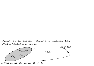
A key point of this section is to represent a sought-after CLF outside the sublevel set $\Omega_{c}$ as the value function in an exit-time optimal control problem, stated with respect to the target set $l_{c}$ and the constant terminal cost $\,V_{\mathrm{loc}}(x)=c\,$ for $x\in l_{c}$ (see Fig. 1):

(21) $$V(x_{0})\>\>\stackrel{{\scriptstyle\mathrm{def}}}{{=}}\>\>\inf_{\begin{subarray}{c}u(\cdot)\,\in\,\mathcal{U}\>\colon\\ T_{\Omega_{c}}(x_{0},\,u(\cdot))\><\>+\infty\end{subarray}}\>\left\{\int\limits_{0}^{T_{\Omega_{c}}(x_{0},\,u(\cdot))}g(x(t;\,x_{0},u(\cdot)),\>u(t))\>\mathrm{d}t\>\,+\>\,c\right\}\quad\forall\,x_{0}\,\in\,G\setminus\Omega_{c}.$$

Assumption 2.15.

The following conditions concerning the running cost $g(\cdot,\cdot)$ hold:

• $\bar{G}\times U\,\ni\,(x,u)\,\,\longmapsto\,\,g(x,u)\>\in\>[0,+\infty)\>$ is a nonnegative continuous function;

• for any $R>0$, there exists $C_{5,R}>0$ such that

  (22) $$|g(x,u)\,-\,g(x^{\prime},u)|\>\,\leqslant\>\,C_{5,R}\,\|x-x^{\prime}\|\quad\forall\>x,x^{\prime}\,\in\,\bar{\mathrm{B}}_{R}(0_{n})\,\cap\,\bar{G}\quad\forall u\in U;$$

• $g(x,u)>0$ for all $\,x\,\in\,G\setminus\{0_{n}\}\,$ and $u\in U$;

• $C_{6}\>\,\stackrel{{\scriptstyle\mathrm{def}}}{{=}}\>\,\inf\>\{g(x,u)\>\colon\>x\,\in\,G\,\setminus\,\mathrm{int}\,\Omega_{c},\>\>u\in U\}\>\,>\>\,0$.

Proposition 2.16.

Under Assumptions 2.1, 2.3, 2.7 and 2.15, the following relations hold for the value function (21):

(23) $$V(x_{0})\,=\,+\infty\quad\forall\,x_{0}\,\in\,G\setminus\mathcal{D}_{0},$$

(24) $$V(x_{0})\,>\,c\quad\forall\,x_{0}\,\in\,\mathcal{D}_{0}\setminus\Omega_{c}.$$

Proof.

The property (23) is clear due to the definition (21) and Proposition 2.14. For establishing (24), let us take $\,x_{0}\,\in\,\mathcal{D}_{0}\setminus\Omega_{c}\,$ and show that

(25) $$\mathcal{T}_{\Omega_{c}}(x_{0})\>\,\stackrel{{\scriptstyle\mathrm{def}}}{{=}}\>\,\inf_{u(\cdot)\,\in\,\mathcal{U}}\>T_{\Omega_{c}}(x_{0},u(\cdot))\>\,>\>\,0.$$

Assume $\,\mathcal{T}_{\Omega_{c}}(x_{0})=0$. Then there exist a number $T>0$ and a sequence $\,\left\{u^{(k)}(\cdot)\right\}_{k=1}^{\infty}\subset\mathcal{U}\,$ such that $\>T^{(k)}\>\stackrel{{\scriptstyle\mathrm{def}}}{{=}}\>T_{\Omega_{c}}\left(x_{0},\,u^{(k)}(\cdot)\right)\>\leqslant\>T\>$ for all $k\in\mathbb{N}$ and $\>\lim_{k\,\to\,\infty}\,T^{(k)}\,=\,0$. According to Remark 2.2, the reachable set

$$X_{T}(x_{0})\>\>\stackrel{{\scriptstyle\mathrm{def}}}{{=}}\>\>\{x(t;\,x_{0},u(\cdot))\>\colon\>t\in[0,T],\>\>u(\cdot)\in\mathcal{U}\}\>\>\subseteq\>\>G$$

is bounded. Since $f(\cdot,\cdot)$ is continuous and $U$ is compact, one has

$$M_{T}(x_{0})\>\,\stackrel{{\scriptstyle\mathrm{def}}}{{=}}\>\,\max_{x\,\in\,\overline{X_{T}(x_{0})},\>\>u\,\in\,U}\>\|f(x,u)\|\>\,<\>\,+\infty.$$

Hence,

$$\begin{array}[]{c}x\left(T^{(k)};\>x_{0},\,u^{(k)}(\cdot)\right)\>\,\in\>\,\Omega_{c}\quad\forall k\in\mathbb{N},\\ 0\>\>\leqslant\>\>\lim\limits_{k\,\to\,\infty}\>\left\|x\left(T^{(k)};\>x_{0},\,u^{(k)}(\cdot)\right)\,\,-\,\,x_{0}\right\|\>\>\leqslant\>\>M_{T}(x_{0})\>\lim\limits_{k\,\to\,\infty}\,T^{(k)}\>\,=\>\,0,\end{array}$$

which contradicts with $x_{0}\notin\Omega_{c}$. This implies (25). From (21), (25) and Item 4 of Assumption 2.15, one obtains $\>V(x_{0})-c\>\geqslant\>C_{6}\,\mathcal{T}_{\Omega_{c}}(x_{0})\>>\>0$. ∎

It is reasonable to extend the function (21) to $\Omega_{c}$ by

(26) $$V(x_{0})\,\stackrel{{\scriptstyle\mathrm{def}}}{{=}}\,V_{\mathrm{loc}}(x_{0})\quad\forall x_{0}\in\Omega_{c}$$

(see Fig. 1).

Proposition 2.17.

Let Assumptions 2.1, 2.3, 2.7 and 2.15 hold, and consider the function $V(\cdot)$ defined by (21) and (26). The following properties hold:

$$\begin{array}[]{c}V(x_{0})\,<\,+\infty\quad\forall x_{0}\in\mathcal{D}_{0},\\ V(x_{0})\,=\,+\infty\quad\forall\,x_{0}\,\in\,G\setminus\mathcal{D}_{0},\\ V(x_{0})\,=\,V_{\mathrm{loc}}(x_{0})\,<\,c\quad\forall\,x_{0}\,\in\,\mathrm{int}\,\Omega_{c},\\ V(x_{0})\,=\,V_{\mathrm{loc}}(x_{0})\,=\,c\quad\forall\,x_{0}\,\in\,l_{c}=\partial\Omega_{c},\\ V(x_{0})\,>\,c\quad\forall\,x_{0}\,\in\,G\setminus\Omega_{c},\\ V_{\mathrm{loc}}(x_{0})\,>\,c\quad\forall\,x_{0}\,\in\,\Omega\setminus\Omega_{c}.\end{array}$$

Proof.

These relations can be directly obtained by using Definition 2.4, Assumption 2.7, Remark 2.9, and Proposition 2.16. ∎

One more technical assumption will be required below.

Assumption 2.18.

There exist positive constants $C_{7},C_{8}$ such that

$$g(x,u)\>\geqslant\>C_{8}\,\|f(x,u)\|\quad\forall\,x\,\in\,G\setminus\mathrm{B}_{C_{7}}(0_{n})\quad\forall u\in U.$$

2.2 Main result

The main result of this section (Theorem 2.20) indicates that, under the adopted assumptions, the concatenation of the local CLF in $\Omega_{c}$ with the value function for the exit-time optimal control problem (21) is a global CLF in the whole domain of asymptotic null-controllability. Before verifying the main result, let us establish some auxiliary properties.

Proposition 2.19.

Under Assumptions 2.1, 2.3, 2.7, 2.15 and 2.18, the following properties hold for the function $V(\cdot)$ defined by (21) and (26):

• $V(\cdot)$ is locally Lipschitz continuous in $\mathcal{D}_{0}$;

• the restriction of $V(\cdot)$ to $\mathcal{D}_{0}\setminus\Omega_{c}$ solves the HJB equation

  $$\max_{u\,\in\,U}\>\{-\left<\mathrm{D}V(x),\,f(x,u)\right>\>-\>g(x,u)\}\>\>=\>\>0,\quad x\,\in\,\mathcal{D}_{0}\setminus\Omega_{c},$$

  in the viscosity sense;

• for any sequence $\>\left\{x^{(k)}\right\}_{k=1}^{\infty}\,\subset\,\mathcal{D}_{0}\>$ satisfying either $\>\lim_{k\,\to\,\infty}\,x^{(k)}\,=\,x^{\prime}\,\in\,\partial\mathcal{D}_{0}\>$ or $\>\lim_{k\,\to\,\infty}\,\left\|x^{(k)}\right\|\,=\,+\infty,\>$ one has $\>\lim_{k\,\to\,\infty}\,V\left(x^{(k)}\right)\,=\,+\infty$.

Proof.

For verifying Items 1, 2, as well as Item 3 for $\>\lim_{k\,\to\,\infty}\,x^{(k)}\,=\,x^{\prime}\,\in\,\partial\mathcal{D}_{0},\>$ it suffices to use [64, Remark 8.1.6] and the reasonings in [64, the proofs of Theorem 8.2.5, Theorem 8.1.8 and Proposition 8.2.6]. As in the proof of Proposition 2.14, Items 4 and 5 of Assumption 2.1 replace the requirement that $f(\cdot,u)$ should satisfy the global Lipschitz condition uniformly with respect to $u\in U$.

It remains to prove Item 3 in case $\>\lim_{k\,\to\,\infty}\,\left\|x^{(k)}\right\|\,=\,+\infty$. Consider such a sequence $\>\left\{x^{(k)}\right\}_{k=1}^{\infty}\,\subset\,\mathcal{D}_{0}$. In line with Assumption 2.18 and the compactness of $\Omega_{c}$, there exists a constant $C^{\prime}_{7}\geqslant C_{7}$ satisfying

$$\begin{array}[]{c}\Omega_{c}\,\subseteq\,\mathrm{B}_{C^{\prime}_{7}}(0_{n}),\\ g(x,u)\>\geqslant\>C_{8}\,\|f(x,u)\|\quad\forall\,x\,\in\,G\setminus\mathrm{B}_{C^{\prime}_{7}}(0_{n})\quad\forall u\in U.\end{array}$$

Denote

$$T_{k}(u(\cdot))\>\>\stackrel{{\scriptstyle\mathrm{def}}}{{=}}\>\>\inf\>\left\{T\in[0,+\infty)\>\colon\>\,x\left(T;\>x^{(k)},\,u(\cdot)\right)\>\in\>\bar{\mathrm{B}}_{C^{\prime}_{7}}(0_{n})\right\}\quad\forall u(\cdot)\in\mathcal{U}\quad\forall k\in\mathbb{N}.$$

Then one has

$$V\left(x^{(k)}\right)\>\>> \inf_{\begin{subarray}{c}u(\cdot)\,\in\,\mathcal{U}\>\colon\\ T_{k}(u(\cdot))\><\>+\infty\end{subarray}}\>\left\{\int\limits_{0}^{T_{k}(u(\cdot))}g\left(x\left(t;\>x^{(k)},\,u(\cdot)\right),\>u(t)\right)\>\mathrm{d}t\right\}$$

$$\geqslant C_{8}\>\inf_{\begin{subarray}{c}u(\cdot)\,\in\,\mathcal{U}\>\colon\\ T_{k}(u(\cdot))\><\>+\infty\end{subarray}}\>\left\{\int\limits_{0}^{T_{k}(u(\cdot))}\left\|f\left(x\left(t;\>x^{(k)},\,u(\cdot)\right),\>u(t)\right)\right\|\>\mathrm{d}t\right\}$$

$$\geqslant C_{8}\>\inf_{\begin{subarray}{c}u(\cdot)\,\in\,\mathcal{U}\>\colon\\ T_{k}(u(\cdot))\><\>+\infty\end{subarray}}\>\left\|x\left(T_{k}(u(\cdot));\>x^{(k)},\,u(\cdot)\right)\>-\>x^{(k)}\right\|$$

$$\geqslant C_{8}\>\left(\left\|x^{(k)}\right\|\,-\,C^{\prime}_{7}\right)$$

for all $k\in\mathbb{N}$. Together with $\>\lim_{k\,\to\,\infty}\,\left\|x^{(k)}\right\|\,=\,+\infty,\>$ this leads to $\>\lim_{k\,\to\,\infty}\,V\left(x^{(k)}\right)\,=\,+\infty$. ∎

Theorem 2.20.

Let Assumptions 2.1, 2.3, 2.7, 2.15 and 2.18 hold. The function $V(\cdot)$ defined by (21) and (26) is a CLF for the system (1) in $\mathcal{D}_{0}$, i. e., the restriction of this function to $\mathcal{D}_{0}$ is a continuous, proper, positive definite and such that the infinitesimal decrease condition

(27) $$\inf_{u\,\in\,U}\>\partial^{-}V(x;\,f(x,u))\>\,\leqslant\>\,-W(x)\quad\forall x\in\mathcal{D}_{0}$$

holds with some continuous and positive definite function $\>W\,\colon\,\mathcal{D}_{0}\to[0,+\infty)$. Furthermore, $V(\cdot)$ is locally Lipschitz continuous in $\mathcal{D}_{0}$ and therefore differentiable almost everywhere in $\mathcal{D}_{0}$ (with respect to the Lebesgue measure in $\mathbb{R}^{n}$).

Proof.

In line with Item 1 of Proposition 2.19, $V(\cdot)$ is locally Lipschitz continuous in $\mathcal{D}_{0}$, and it is differentiable almost everywhere in $\mathcal{D}_{0}$ due to Rademacher’s theorem. The positive definiteness of $V(\cdot)$ directly follows from Proposition 2.16 and the positive definiteness of $V_{\mathrm{loc}}(\cdot)$.

Let us show that $V(\cdot)$ is proper. According to the relation (23) and Item 3 of Proposition 2.19, it suffices to verify the properness of the restriction of $V(\cdot)$ to $\mathcal{D}_{0}$. The continuity of the latter implies that the preimages of closed sets are closed. Again due to Item 3 of Proposition 2.19, the considered restriction is also such that the preimages of bounded sets are bounded. One consequently obtains the compactness of the preimages of compact sets, which means properness.

It remains to establish the infinitesimal decrease condition (27) with an appropriate function $W(\cdot)$.

Since the function $\>W_{\mathrm{loc}}\,\colon\,\Omega\to[0,+\infty)\>$ (introduced in Item 2 of Assumption 2.7) is continuous and the set $\Omega_{c}\subset\Omega$ is compact, Tietze’s extension theorem (see, e. g., [66, Theorem 5.2.1]) ensures the existence of a continuous function $\>W_{1}\colon\,\mathbb{R}^{n}\to\mathbb{R}\>$ satisfying $\,W_{1}(x)=W_{\mathrm{loc}}(x)\,$ for all $x\in\Omega_{c}$. Bearing in mind also the positive definiteness of $W_{\mathrm{loc}}(\cdot)$ and the compactness of the boundary $l_{c}=\partial\Omega_{c}$ that does not contain $0_{n}$, one concludes $\>\min_{x\,\in\,l_{c}}\,W_{\mathrm{loc}}(x)\>>\>0$. Hence, the function

$$W_{2}(x)\>\>\stackrel{{\scriptstyle\mathrm{def}}}{{=}}\>\>\begin{cases}W_{\mathrm{loc}}(x),&x\in\Omega_{c},\\ \max\,\left\{W_{1}(x),\,\,\min\limits_{\xi\,\in\,l_{c}}\,W_{\mathrm{loc}}(\xi)\right\},&x\,\in\,\mathbb{R}^{n}\setminus\Omega_{c},\end{cases}$$

is continuous and positive definite. Now take

(28) $$W(x)\>\,\stackrel{{\scriptstyle\mathrm{def}}}{{=}}\>\,\min\,\left\{W_{2}(x),\,\,\min_{u\,\in\,U}\,g(x,u)\right\}\quad\forall x\in\mathcal{D}_{0}.$$

The compactness of $U$ and Items 1, 3 of Assumption 2.15 yield that the function $\>G\,\ni\,x\>\longmapsto\>\min_{u\,\in\,U}\,g(x,u)\>$ is continuous everywhere in $G$ and positive for all $\,x\,\in\,G\setminus\{0_{n}\}$. Thus, (28) is a continuous and positive definite function.

In order to establish the condition (27) with the selected $W(\cdot)$, it suffices to verify this Dini form for $x\in\Omega_{c}$ and the related viscosity form for $\,x\,\in\,\mathcal{D}_{0}\setminus\Omega_{c}\,$ (recall Remark 2.6).

For $\,x\,\in\,\mathrm{int}\,\Omega_{c},\,$ the inequality in (27) holds due to Assumption 2.7. For $\,x\,\in\,\mathcal{D}_{0}\setminus\Omega_{c},\,$ Item 2 of Proposition 2.19 implies the viscosity form of the infinitesimal decrease condition:

$$\max_{u\,\in\,U}\>\{-\left<\zeta,\,f(x,u)\right>\}\>\,-\>\,W(x)$$

$$\qquad\geqslant\>\>\max_{u\,\in\,U}\>\{-\left<\zeta,\,f(x,u)\right>\}\>\,-\>\,\min_{u\,\in\,U}\,g(x,u)$$

$$\qquad\geqslant\>\>\max_{u\,\in\,U}\>\{-\left<\zeta,\,f(x,u)\right>\>-\>g(x,u)\}\>\>\geqslant\>\>0$$

$$\forall\,\zeta\,\in\,\mathrm{D}^{-}V(x).$$

It therefore remains to prove the inequality in (27) for $\,x\,\in\,l_{c}=\partial\Omega_{c}$.

Let $x\in l_{c}$. Due to the local Lipschitz continuity of $V(\cdot)$ and $V_{\mathrm{loc}}(\cdot)$ in $\mathcal{D}_{0}$ and $\Omega$, respectively, the following representations for the lower Dini derivatives hold (see, e. g., [64, Remark 3.1.4]):

(29) $$\partial^{-}V(x;\zeta)\>\,=\>\,\liminf_{\lambda\,\to\,+0}\>\frac{V(x+\lambda\zeta)\,-\,V(x)}{\lambda}\,,$$

$$\partial^{-}V_{\mathrm{loc}}(x;\zeta)\>\,=\>\,\liminf_{\lambda\,\to\,+0}\>\frac{V_{\mathrm{loc}}(x+\lambda\zeta)\,-\,V_{\mathrm{loc}}(x)}{\lambda}$$

$$\forall\zeta\in\mathbb{R}^{n}.$$

Introduce the control subset

$$U_{x}\>\>\stackrel{{\scriptstyle\mathrm{def}}}{{=}}\>\>\left\{u\in U\>\,\colon\>\,\mbox{there exists a sequence $\,\{\lambda_{k}\}_{k=1}^{\infty}\subset(0,+\infty)\,$ such that}\right.$$

$$\left.\mbox{$\lim\limits_{k\,\to\,\infty}\,\lambda_{k}\,=\,0\,$ and $\>x\,+\,\lambda_{k}\,f(x,u)\>\in\>\Omega_{c}\>$ for all $k\in\mathbb{N}$}\right\},$$

which is nonempty by virtue of Proposition 2.11. With the help of Proposition 2.17 and the property (29), one obtains

$$\begin{array}[]{c}\inf\limits_{u\,\in\,U_{x}}\>\partial^{-}V(x;\,f(x,u))\>\,\leqslant\>\,0,\quad\inf\limits_{u\>\in\>U\,\setminus\,U_{x}}\>\partial^{-}V(x;\,f(x,u))\>\,\geqslant\>\,0,\\ \inf\limits_{u\,\in\,U_{x}}\>\partial^{-}V_{\mathrm{loc}}(x;\,f(x,u))\>\,\leqslant\>\,0,\quad\inf\limits_{u\>\in\>U\,\setminus\,U_{x}}\>\partial^{-}V_{\mathrm{loc}}(x;\,f(x,u))\>\,\geqslant\>\,0,\end{array}$$

and

$$\inf_{u\,\in\,U}\>\partial^{-}V(x;\,f(x,u))\>\,=\>\,\inf_{u\,\in\,U_{x}}\>\partial^{-}V(x;\,f(x,u))$$

$$\qquad=\>\,\inf_{u\,\in\,U_{x}}\>\partial^{-}V_{\mathrm{loc}}(x;\,f(x,u))\>\,=\>\,\inf_{u\,\in\,U}\>\partial^{-}V_{\mathrm{loc}}(x;\,f(x,u)).$$

Together with (3), this leads to

$$\inf_{u\,\in\,U}\>\partial^{-}V(x;\,f(x,u))\>\,\leqslant\>\,-W_{\mathrm{loc}}(x)\>\,\leqslant\>\,-W(x)$$

and thereby completes the proof. ∎

2.3 Investigation of the exit-time optimal control problem

As was shown in the previous subsection, if one can find a suitable local CLF $V_{\mathrm{loc}}(\cdot)$ and the conditions of Theorem 2.20 are fulfilled, the value function in the exit-time optimal control problem (21) extends the local CLF outside the sublevel set $\Omega_{c}$, so that the resulting function $V(\cdot)$ becomes a global CLF in the whole domain of asymptotic null-controllability $\mathcal{D}_{0}$.

In order to verify the existence of optimal control strategies and to use necessary optimality conditions (Pontryagin’s principle) for the exit-time problem (21) with $\,x_{0}\,\in\,\mathcal{D}_{0}\setminus\Omega_{c},\,$ let us reformulate it as

(30) $$V(x_{0})\>\>\stackrel{{\scriptstyle\mathrm{def}}}{{=}}\>\>\inf_{\begin{subarray}{c}u(\cdot)\,\in\,\mathcal{U},\>\>T\,\in\,[0,+\infty)\>\colon\\ x(T;\>x_{0},\,u(\cdot))\,\,\in\,\,\Omega_{c}\end{subarray}}\>\left\{\int\limits_{0}^{T}g(x(t;\,x_{0},u(\cdot)),\>u(t))\>\mathrm{d}t\>\,+\>\,c\right\}\quad\forall\,x_{0}\,\in\,G\setminus\Omega_{c}.$$

It is easy to see that (21) and (30) are equivalent under Assumptions 2.1, 2.3, 2.7 and 2.15. Some additional conditions also need to be imposed.

Assumption 2.21.

The set

$$\left\{(f(x,u),\,y)\>\in\>\mathbb{R}^{n}\times\mathbb{R}\>\colon\>u\in U,\>\>y\,\geqslant\,g(x,u)\right\}$$

is convex for every $x\in\bar{G}$.

Remark 2.22.

Assumption 2.21 strengthens Assumption 2.3. One can easily verify that a sufficient condition for the fulfillment of Assumption 2.21 is the convexity of the set

$$\left\{(f(x,u),\,g(x,u))\>\in\>\mathbb{R}^{n}\times\mathbb{R}\>\colon\>u\in U\right\}$$

for all $x\in\bar{G}$. ∎

Assumption 2.23.

The functions $\>G\,\ni\,x\>\,\longmapsto\>\,f(x,u)\,\in\,\mathbb{R}^{n}\>$ and $\>G\,\ni\,x\>\,\longmapsto\>\,g(x,u)\,\in\,[0,+\infty)\>$ are continuously differentiable for every $u\in U$.

Theorem 2.24.

Let Assumptions 2.1, 2.7, 2.15 and 2.21 hold. For any fixed initial state $\,x_{0}\,\in\,\mathcal{D}_{0}\setminus\Omega_{c},\,$ there exists an optimal control strategy for the exit-time problem (21) or, equivalently, for (30).

Proof.

Consider the optimal control problem (21) or (30) with a fixed initial state $\,x_{0}\,\in\,\mathcal{D}_{0}\setminus\Omega_{c}$. In line with Proposition 2.17, one has $\,V(x_{0})<+\infty$. Fix an arbitrary $\varepsilon>0$. By $\mathcal{U}_{\varepsilon}(x_{0})$, denote the set of all $u(\cdot)\in\mathcal{U}$ for which the cost is not greater than $\,V(x_{0})+\varepsilon$. The control subclass $\mathcal{U}_{\varepsilon}(x_{0})$ obviously contains a minimizing sequence. Recall also the notation (20). By the definition of $\mathcal{U}_{\varepsilon}(x_{0})$, one has $\>T_{\Omega_{c}}(x_{0},u(\cdot))\,<\,+\infty\>$ for all $\,u(\cdot)\,\in\,\mathcal{U}_{\varepsilon}(x_{0})$. If one proves that the integral funnel

(31) $$\{(t,\>x(t;\,x_{0},u(\cdot)))\>\,\colon\>\,t\>\in\>[0,\,T_{\Omega_{c}}(x_{0},u(\cdot))],\>\>\,u(\cdot)\,\in\,\mathcal{U}_{\varepsilon}(x_{0})\}$$

is contained in some compact set $K\subset\mathbb{R}^{n+1}$, then including the constraint that admissible integral trajectories should lie in $K$ will not change the infimum in the considered optimal control problem, while this will allow for using the general existence theorem of [40, §9.3]. Thus, it remains to establish the boundedness of (31). According to Remark 2.2, it suffices to verify that the set of exit times $\>\{T_{\Omega_{c}}(x_{0},u(\cdot))\>\colon\>u(\cdot)\,\in\,\mathcal{U}_{\varepsilon}(x_{0})\}\>$ is bounded. Due to the definition of $\mathcal{U}_{\varepsilon}(x_{0})$ and Item 4 of Assumption 2.15, any $\,u(\cdot)\,\in\,\mathcal{U}_{\varepsilon}(x_{0})\,$ satisfies

$$C_{6}\>T_{\Omega_{c}}(x_{0},\,u(\cdot))\>\,+\>\,c\>\>\leqslant\>\>\int\limits_{0}^{T_{\Omega_{c}}(x_{0},\,u(\cdot))}g(x(t;\,x_{0},u(\cdot)),\>u(t))\>\mathrm{d}t\>\,+\>\,c\>\>\leqslant\>\>V(x_{0})\,+\,\varepsilon$$

with a constant $C_{6}>0$, which leads to the estimate

$$T_{\Omega_{c}}(x_{0},\,u(\cdot))\>\leqslant\>\frac{V(x_{0})\,+\,\varepsilon\,-\,c}{C_{6}}$$

and therefore completes the proof. ∎

Theorem 2.25.

(Pontryagin’s principle; see, e. g., [40, §5.1, §4.2 (emphasize Remark 10), §4.4.B], [41, §2.4]) Let Assumptions 2.1, 2.7, 2.15, 2.21 and 2.23 hold. Consider an optimal control strategy $u^{*}(\cdot)\in\mathcal{U}$ in the exit-time problem (21) or, equivalently, in (30) for a fixed initial state $\,x_{0}\,\in\,\mathcal{D}_{0}\setminus\Omega_{c}$. Denote $\>T^{*}\,\stackrel{{\scriptstyle\mathrm{def}}}{{=}}\,T_{\Omega_{c}}(x_{0},\,u^{*}(\cdot))\,<\,+\infty,\>$ and let

$$[0,T^{*}]\>\ni\>t\>\>\longmapsto\>\>x^{*}(t)\>\stackrel{{\scriptstyle\mathrm{def}}}{{=}}\>x(t;\,x_{0},u^{*}(\cdot))\>\in\>G$$

be the corresponding optimal state trajectory. Moreover, introduce the Hamiltonian:

(32) $$H(x,u,p,\tilde{p})\>\,\stackrel{{\scriptstyle\mathrm{def}}}{{=}}\>\,\left<p,f(x,u)\right>\>+\>\tilde{p}\,g(x,u),$$

$$\mathcal{H}(x,p,\tilde{p})\>\,\stackrel{{\scriptstyle\mathrm{def}}}{{=}}\>\,\min_{u^{\prime}\,\in\,U}\,H(x,u^{\prime},p,\tilde{p})$$

$$\forall\>(x,u,p,\tilde{p})\>\in\>G\times U\times\mathbb{R}^{n}\times\mathbb{R}.$$

Then there exist a function $\>p^{*}\colon\,[0,T^{*}]\to\mathbb{R}^{n}\>$ and a constant $\tilde{p}^{*}\geqslant 0$ such that the following properties hold:

• $(p^{*}(t),\tilde{p}^{*})\,\neq\,0_{n+1}\>$ for every $t\in[0,T^{*}]$;

• $(x^{*}(\cdot),p^{*}(\cdot))\,$ is an absolutely continuous solution of the characteristic boundary value problem

  (33) $$\left\{\begin{aligned} &\dot{x^{*}}(t)\>\>=\>\>\mathrm{D}_{p}H(x^{*}(t),\,u^{*}(t),\,p^{*}(t),\,\tilde{p}^{*})\>\>=\>\>f(x^{*}(t),\,u^{*}(t)),\\ &\dot{p^{*}}(t)\>\>=\>\>-\mathrm{D}_{x}H(x^{*}(t),\,u^{*}(t),\,p^{*}(t),\,\tilde{p}^{*})\\ &\qquad\>\>=\>\>-(\mathrm{D}_{x}f(x^{*}(t),\,u^{*}(t)))^{\top}\>p^{*}(t)\>\,-\>\,\tilde{p}^{*}\>\mathrm{D}_{x}g(x^{*}(t),\,u^{*}(t)),\\ &t\,\in\,[0,T^{*}],\\ &x^{*}(0)\,=\,x_{0},\\ &x^{*}(T^{*})\,\in\,l_{c},\quad p^{*}(T^{*})\,\in\,\mathrm{N}(x^{*}(T^{*});\,\Omega_{c})\end{aligned}\right.$$

  (the notation for normal cones was described in the introduction);

• the Hamiltonian minimum condition

  (34) $$H(x^{*}(t),\,u^{*}(t),\,p^{*}(t),\,\tilde{p}^{*})\>\,=\>\,\mathcal{H}(x^{*}(t),\,p^{*}(t),\,\tilde{p}^{*})$$

  is satisfied for almost all $\,t\in[0,T^{*}]\,$ (with respect to the Lebesgue measure in $\mathbb{R}$);

• the Hamiltonian vanishes along the optimal characteristic trajectory, i. e.,

  (35) $$\mathcal{H}(x^{*}(t),\,p^{*}(t),\,\tilde{p}^{*})\>\equiv\>0\quad\forall t\in[0,T^{*}].$$

Remark 2.26.

Since the Hamiltonian (32) is positive homogeneous of degree $1$ with respect to $(p,\tilde{p})$, it suffices to consider only the two cases $\tilde{p}^{*}=0$ and $\tilde{p}^{*}=1$ in Theorem 2.25. The case $\tilde{p}^{*}=0$ is called abnormal. ∎

For handling the infinite value $+\infty$, consider the Kruzhkov transformed function

(36) $$v(x_{0})\>\,\stackrel{{\scriptstyle\mathrm{def}}}{{=}}\>\,1\,-\,e^{-V(x_{0})}\>\,\in\>\,[0,1]\quad\forall x_{0}\in G$$

with the convention $\,e^{-(+\infty)}\stackrel{{\scriptstyle\mathrm{def}}}{{=}}0$. Note that the function $\>\mathbb{R}\ni\xi\>\longmapsto\>1-e^{-\xi}\>$ vanishes at $\xi=0$, tends to $1$ as $\xi\to+\infty$, strictly increases, and is infinitely differentiable.

Theorem 2.27.

Let Assumptions 2.1, 2.3, 2.7 and 2.15 hold, and consider the functions $V(\cdot)$, $v(\cdot)$ defined by (21), (26), (36). The domain of asymptotic null-controllability can be represented as

$$\mathcal{D}_{0}\>\>=\>\>\{x_{0}\in G\>\colon\>V(x_{0})\,<\,+\infty\}\>\>=\>\>\{x_{0}\in G\>\colon\>v(x_{0})\,<\,1\}.$$

Proof.

It suffices to recall Proposition 2.17. ∎

Introduce also the set-valued extremal control map:

(37) $$U^{*}(x,p,\tilde{p})\>\,\stackrel{{\scriptstyle\mathrm{def}}}{{=}}\>\,\mathrm{Arg}\min_{u\,\in\,U}\,H(x,u,p,\tilde{p})\quad\forall\>(x,p,\tilde{p})\>\in\>G\times\mathbb{R}^{n}\times\mathbb{R}.$$

As was discussed in [33, 56, 57], characteristic boundary value problems, such as (33), may admit multiple solutions, some of which may not be optimal, and it is therefore relevant to parametrize the characteristic fields with respect to the extended initial adjoint vector ($(p_{0},\tilde{p}^{*})$ in case of (33)) and to solve the related Cauchy problems. Solutions of the latter are unique if, for example, the absence of the abnormal case $\tilde{p}^{*}=0$ is verified and the running cost is regularized by adding an appropriate control-dependent term, so that the extremal control map takes only singleton values along the characteristic trajectories.

Taking that into account, the next theorem reduces the computation of the transformed value function (36) at any selected state $\,x_{0}\,\in\,\mathcal{D}_{0}\setminus\Omega_{c}\,$ to a finite-dimensional optimization problem with respect to the unknown initial data $(p_{0},\tilde{p}^{*})$ for the characteristic system. For certain classes of optimal control problems with fixed finite horizons and free terminal states, some related techniques were previously proposed and tested in [36, 37, 33]. Theoretical results regarding the construction of global CLFs via exit-time optimal control and Pontryagin’s characteristics were initially formulated in the conference papers [56, 57], while the current work provides their extension with detailed proofs, discussions, and practical developments.

Theorem 2.28.

Let Assumptions 2.1, 2.7, 2.15, 2.21 and 2.23 hold. For any initial state $\,x_{0}\,\in\,\mathcal{D}_{0}\setminus\Omega_{c},\,$ the Kruzhkov transformed value $v(x_{0})$ defined by (20), (21), (36) is the minimum of

(38) $$1\>\>-\>\>\exp\left\{-\int\limits_{0}^{T_{\Omega_{c}}(x_{0},\,u^{*}(\cdot))}g(x^{*}(t),\,u^{*}(t))\>\mathrm{d}t\>\,-\>\,c\right\}$$

over the solutions of the characteristic Cauchy problems

(39) $$\left\{\begin{aligned} &\dot{x^{*}}(t)\>\>=\>\>\mathrm{D}_{p}H(x^{*}(t),\,u^{*}(t),\,p^{*}(t),\,\tilde{p}^{*})\>\>=\>\>f(x^{*}(t),\,u^{*}(t)),\\ &\dot{p^{*}}(t)\>\>=\>\>-\mathrm{D}_{x}H(x^{*}(t),\,u^{*}(t),\,p^{*}(t),\,\tilde{p}^{*})\\ &\qquad\>\>=\>\>-(\mathrm{D}_{x}f(x^{*}(t),\,u^{*}(t)))^{\top}\>p^{*}(t)\>\,-\>\,\tilde{p}^{*}\>\mathrm{D}_{x}g(x^{*}(t),\,u^{*}(t)),\\ &u^{*}(t)\>\in\>U^{*}(x^{*}(t),\,p^{*}(t),\,\tilde{p}^{*}),\\ &t\>\,\in\>\,I(x_{0},\,u^{*}(\cdot))\>\,\stackrel{{\scriptstyle\mathrm{def}}}{{=}}\>\,\begin{cases}[0,\,T_{\Omega_{c}}(x_{0},\,u^{*}(\cdot))],&T_{\Omega_{c}}(x_{0},\,u^{*}(\cdot))\><\>+\infty,\\ [0,+\infty),&T_{\Omega_{c}}(x_{0},\,u^{*}(\cdot))\>=\>+\infty,\end{cases}\\ &x^{*}(0)\,=\,x_{0},\quad p^{*}(0)\,=\,p_{0},\end{aligned}\right.$$

for all extended initial adjoint vectors

(40) $$(p_{0},\tilde{p}^{*})\>\,\in\>\,\{(p,\tilde{p})\>\colon\>p\in\mathbb{R}^{n},\>\>\tilde{p}\in\{0,1\}\}.$$

Moreover, the same value is obtained when minimizing over the bounded set

(41) $$(p_{0},\tilde{p}^{*})\>\,\in\>\,\{(p,\tilde{p})\>\in\>\mathbb{R}^{n}\times\mathbb{R}\>\colon\>\|(p,\tilde{p})\|\>=\>1,\>\>\,\tilde{p}\geqslant 0\},$$

or even over its subset

(42) $$(p_{0},\tilde{p}^{*})\>\,\in\>\,\{(p,\tilde{p})\>\in\>\mathbb{R}^{n}\times\mathbb{R}\>\colon\>\|(p,\tilde{p})\|\>=\>1,\>\>\,\tilde{p}\geqslant 0,\>\>\,\mathcal{H}(x_{0},p,\tilde{p})\>=\>0\}.$$

Proof.

The first statement directly follows from Theorems 2.24, 2.25, Remark 2.26 and the fact that, compared to the boundary value problems (33), (34), the Cauchy problems (39), (40) generate a wider characteristic field (due to the absence of the transversality condition on the terminal adjoint vector).

Since the Hamiltonian is positive homogeneous of degree $1$ with respect to $\left(p,\tilde{p}\right)$, the extremal control map (37) satisfies

$$U^{*}\left(x,p,\tilde{p}\right)\>\,=\>\,U^{*}\left(x,\,\lambda\,p,\,\lambda\,\tilde{p}\right)\quad\forall\lambda>0\quad\forall\>\left(x,p,\tilde{p}\right)\>\in\>G\times\mathbb{R}^{n}\times\mathbb{R},$$

and the state components of the characteristic trajectories do not change after multiplying $\left(p_{0},\tilde{p}^{*}\right)$ by any positive number. Together with the Hamiltonian vanishing condition (35) in Theorem 2.25, this yields the second statement. ∎

Besides, let us separately formulate the well-known Hamiltonian conservation property as applied to (39). For convenience, its proof is given in Subsection A.1.2 of Online_App the appendix.

Proposition 2.29.

Under the conditions of Theorem 2.28, the Hamiltonian is conserved along any solution of the characteristic Cauchy problem (39) with $\>(x_{0},p_{0},\tilde{p}^{*})\>\in\>G\,\times\,\mathbb{R}^{n}\,\times\,[0,+\infty)$.

Theorems 2.20, 2.24, 2.25, 2.27 and 2.28 form the theoretical basis of a curse-of-dimensionality-free approach to approximating global CLFs and feedback stabilization. A number of related practical aspects are discussed in Section 4 below and also in Section A.2 of Online_App the appendix, while the next section modifies the theoretical constructions of the current section for the case when an appropriate local CLF is not available.

3 Approximation of a global CLF in case when an appropriate local CLF is not available

If linearization based techniques for building quadratic local CLFs (see Subsection A.2.1 of Online_App the appendix) cannot be applied to a particular system, it may be very difficult to obtain a suitable local CLF. Even if the conditions of Theorems 2.20, 2.24, 2.27 and 2.28 hold with an explicitly found nonsmooth local CLF and some software implementation of a direct approximation method (e. g., one of the toolkits mentioned in Subsection A.2.3 of Online_App the appendix) can be launched for the corresponding exit-time optimal open-loop control problems, the nonsmoothness may still cause significant numerical issues. This section describes the theoretical constructions that were previously introduced in the conference paper [56] and could help to approximate global CLFs for some classes of nonlinear control systems without using any local CLFs. Here we also discuss the proofs omitted in [56] and provide a qualitative comparison with the constructions of Section 2.

Let us consider the control system (1) and indicate the required assumptions.

Since it is not asserted that a suitable local CLF can be obtained, some new conditions on the running cost $g(\cdot,\cdot)$ have to be imposed (they do not appear in Section 2). Furthermore, it is convenient to assume the boundedness of the set of pointwise control constraints $U$ from the very beginning (in [56], this was supposed just after Proposition 2.8 stating that the region of asymptotic null-controllability $\mathcal{D}_{0}$ is an open domain, but before Assumption 2.12 introducing the running cost).

First, Assumption 2.1 is adopted. It is also supposed that a local asymptotic null-controllability property holds in a weak or strong form as follows (see [4, Section 2]).

Assumption 3.1.

$0_{m}\in U$, $f(0_{n},0_{m})=0_{n}$, and one of the following two conditions holds (the second condition strengthens the first one and is called the small control property):

• there exist positive constants $r,\bar{u}$ and a function $\,\beta(\cdot,\cdot)\in\mathcal{K}\mathcal{L}\,$ such that $\bar{\mathrm{B}}_{r}(0_{n})\subset G$ and, for any $x_{0}\in\mathrm{B}_{r}(0_{n})$, there is a control strategy $u_{x_{0}}(\cdot)\in\mathcal{U}$ satisfying

  (43) $$\begin{array}[]{c}\left\|u_{x_{0}}(\cdot)\right\|_{L^{\infty}([0,+\infty),\,U)}\>\,\leqslant\>\,\bar{u},\\ \left\|x\left(t;\,x_{0},u_{x_{0}}(\cdot)\right)\right\|\>\,\leqslant\>\,\beta(\|x_{0}\|,t)\quad\forall t\geqslant 0;\end{array}$$

• there exists a constant $r>0$ and a function $\,\beta(\cdot,\cdot)\in\mathcal{K}\mathcal{L}\,$ such that $\bar{\mathrm{B}}_{r}(0_{n})\subset G$ and, for any $x_{0}\in\mathrm{B}_{r}(0_{n})$, there is a control strategy $u_{x_{0}}(\cdot)\in\mathcal{U}$ satisfying

  $$\left\|x\left(t;\,x_{0},u_{x_{0}}(\cdot)\right)\right\|\>+\>\left\|u_{x_{0}}(t)\right\|\>\>\leqslant\>\>\beta(\|x_{0}\|,t)\quad\forall t\geqslant 0$$

  (this implies (43) with $\bar{u}=\beta(r,0)$).

Remark 3.2.

If $\,0_{m}\in\mathrm{int}\,U$, $\,f(0_{n},0_{m})=0_{n},\,$ the function $f(\cdot,\cdot)$ is continuously differentiable, and the linearization

(44) $$\begin{array}[]{c}\dot{x}(t)\>=\>A\,x(t)\,+\,B\,u(t),\quad t\geqslant 0,\quad u(\cdot)\,\in\,\mathcal{U},\\ A\>\stackrel{{\scriptstyle\mathrm{def}}}{{=}}\>\mathrm{D}_{x}f(0_{n},0_{m})\>\in\>\mathbb{R}^{n\times n},\quad B\>\stackrel{{\scriptstyle\mathrm{def}}}{{=}}\>\mathrm{D}_{u}f(0_{n},0_{m})\>\in\>\mathbb{R}^{n\times m},\end{array}$$

of the system (1) is asymptotically null-controllable, then (1) admits a locally stabilizing linear feedback according to [67, §5.8, Theorem 19], and Item 2 of Assumption 3.1 therefore holds. ∎

Remark 3.3.

Due to [68, Proposition 7], $\,\beta(\cdot,\cdot)\in\mathcal{K}\mathcal{L}\,$ implies the existence of two functions $\>\alpha_{1}(\cdot),\alpha_{2}(\cdot)\,\in\,\mathcal{K}_{\infty}\>$ satisfying

(45) $$\beta(\rho,t)\>\leqslant\>\alpha_{2}\left(\alpha_{1}(\rho)\,e^{-t}\right)\quad\forall\rho\geqslant 0\quad\forall t\geqslant 0.$$

For example, if $C_{9},C_{10}$ are positive constants, $\nu(\cdot)\in\mathcal{K}_{\infty}$, and

$$\beta(\rho,t)\>=\>C_{9}\,\nu(\rho)\,e^{-C_{10}\,t}\quad\forall\rho\geqslant 0\quad\forall t\geqslant 0,$$

then one can choose

$$\alpha_{1}(\rho)\>=\>(\nu(\rho))^{1/C_{10}},\quad\alpha_{2}(\rho)\>=\>C_{9}\,\rho^{C_{10}}\quad\forall\rho\geqslant 0\quad\forall t\geqslant 0$$

in order to fulfill the estimate (45) in the equality form. ∎

Proposition 3.4.

[4, Proposition 2.3] Let Assumptions 2.1 and 3.1 hold. The region of asymptotic null-controllability $\mathcal{D}_{0}$ is an open domain containing the closed ball $\bar{\mathrm{B}}_{r}(0_{n})$. Furthermore, $\mathcal{D}_{0}$ is weakly invariant in the sense that, for any $x_{0}\in\mathcal{D}_{0}$, there exists $u_{x_{0}}(\cdot)\in\mathcal{U}$ satisfying $\>x(t;\,x_{0},u_{x_{0}}(\cdot))\,\in\,\mathcal{D}_{0}\>$ for all $t\geqslant 0$.

Next, let us formulate the conditions on the running cost $g(\cdot,\cdot)$ in an infinite-horizon optimal control problem leading to a global CLF in line with the results of [4, Sections 3 and 4].

Assumption 3.5.

Let $\alpha_{2}^{-1}(\cdot)$ be the inverse of the function $\alpha_{2}(\cdot)$ introduced in Remark 3.3, and take the constants $r,\bar{u}$ from Assumption 3.1. The following properties hold:

• $\bar{G}\times U\,\ni\,(x,u)\>\longmapsto\>g(x,u)\,\in\,[0,+\infty)\>$ is a nonnegative continuous function, and, for any $R>0$, there exists $C_{5,R}>0$ satisfying the condition (22) (these are Items 1, 2 of Assumption 2.15);

• for any $R>0$, one has

  $$\inf\>\{g(x,u)\>\colon\>(x,u)\,\in\,\bar{G}\times U,\>\>\|x\|\,\geqslant\,R\}\>\>>\>\>0;$$

• if Item 2 of Assumption 3.1 (the small control property) is not asserted, then there exist positive constants $C_{11},C_{12}$ such that

  (46) $$g(x,u)\>\>\leqslant\>\>C_{11}\>\left(\alpha_{2}^{-1}(\|x\|)\right)^{C_{12}}\quad\forall x\in\bar{\mathrm{B}}_{r}(0_{n})\quad\forall\>u\,\in\,\bar{\mathrm{B}}_{\bar{u}}(0_{m})\,\cap\,U;$$

• if Item 2 of Assumption 3.1 holds, then the condition (46) is weakened to

  $$g(x,u)\>\>\leqslant\>\>C_{11}\>\left(\alpha_{2}^{-1}(\|x\|+\|u\|)\right)^{C_{12}}\quad\forall x\in\bar{\mathrm{B}}_{r}(0_{n})\quad\forall\>u\,\in\,\bar{\mathrm{B}}_{\bar{u}}(0_{m})\,\cap\,U,$$

  where $C_{11},C_{12}$ are positive constants;

• there exists a constant $C_{13}>0$ satisfying

  $$g(x,u)\>\geqslant\>C_{13}\,\|f(x,u)\|\quad\forall\>(x,u)\>\in\>\{(x^{\prime},u^{\prime})\,\in\,\bar{G}\times U\>\colon\>\|x^{\prime}\|\,\geqslant\,2r\>\>\mathrm{or}\>\>\|u^{\prime}\|\,\geqslant\,2\bar{u}\}$$

  (we take $\bar{u}=\beta(r,0)$ if Item 2 of Assumption 3.1 holds).

Note the difference between Items 2–5 of Assumption 3.5 on one hand, and Items 3, 4 of Assumption 2.15 together with Assumption 2.18 on the other.

Introduce the infinite-horizon optimal control problem

(47) $$V_{0}(x_{0})\>\>\stackrel{{\scriptstyle\mathrm{def}}}{{=}}\>\>\inf_{u(\cdot)\,\in\,\mathcal{U}}\>\left\{\int\limits_{0}^{+\infty}g(x(t;\,x_{0},u(\cdot)),\>u(t))\>\mathrm{d}t\right\}\>\>\in\>\>[0,+\infty)\,\cup\,\{+\infty\}\quad\forall x_{0}\in G.$$

Similarly to (36), consider the Kruzhkov transformed value function

(48) $$v_{0}(x_{0})\>\,\stackrel{{\scriptstyle\mathrm{def}}}{{=}}\>\,1\,-\,e^{-V_{0}(x_{0})}\>\,\in\>\,[0,1]\quad\forall x_{0}\in G$$

with the convention $\,e^{-(+\infty)}\stackrel{{\scriptstyle\mathrm{def}}}{{=}}0$.

Similarly to [4, Propositions 3.3, 3.5, 3.6 and Remark 4.2], one can obtain the following result that represents the domain of asymptotic null-controllability $\mathcal{D}_{0}$ via the value functions $V_{0}(\cdot),v_{0}(\cdot)$ and indicates the CLF property for $V_{0}(\cdot)$ in $\mathcal{D}_{0}$.

Theorem 3.6.

Let Assumptions 2.1, 3.1 and Items 1–4 of Assumption 3.5 hold. Then the domain of asymptotic null-controllability is represented as

(49) $$\mathcal{D}_{0}\>\>=\>\>\{x_{0}\in G\>\colon\>V_{0}(x_{0})\,<\,+\infty\}\>\>=\>\>\{x_{0}\in G\>\colon\>v_{0}(x_{0})\,<\,1\}.$$

If, moreover, Item 5 of Assumption 3.5 holds, then the restriction of $V_{0}(\cdot)$ to $\mathcal{D}_{0}$ is a CLF for the system (1), and the following statements in particular hold:

• $V_{0}(\cdot)$ is continuous on $\mathcal{D}_{0}$, $v_{0}(\cdot)$ is continuous on $G$;

• $\{x_{0}\in G\>\colon\>V_{0}(x_{0})\,=\,0\}\>\,=\>\,\{x_{0}\in G\>\colon\>v_{0}(x_{0})\,=\,0\}\>\,=\>\,\{0_{n}\}$;

• for any sequence $\,\left\{x^{(k)}\right\}_{k=1}^{\infty}\subset G\,$ satisfying either

  $$\lim_{k\,\to\,\infty}\,\mathrm{dist}\,\left(x^{(k)},\partial\mathcal{D}_{0}\right)\>=\>0\quad\mathrm{or}\quad\lim_{k\,\to\,\infty}\,\left\|x^{(k)}\right\|\>=\>+\infty,$$

  one also has

  $$\lim_{k\,\to\,\infty}\,V_{0}\left(x^{(k)}\right)\>=\>+\infty\quad\mathrm{and}\quad\lim_{k\,\to\,\infty}\,v_{0}\left(x^{(k)}\right)\>=\>1.$$

The dynamic programming principle for the transformed value function $v_{0}(\cdot)$ can be formulated as follows (see, e. g., [4, Section 3] and [69, Sections 3, 4]).

Proposition 3.7.

Under Assumptions 2.1, 3.1 and Items 1–4 of Assumption 3.5, one has

(50) $$v_{0}(x_{0})\>\>=\>\>\inf\limits_{u(\cdot)\,\in\,\mathcal{U}}\>\inf\limits_{T\,\in\,[0,+\infty)}\>\{1\>\,-\>\,\mu(x_{0},u(\cdot),T)\>\,+\>\,\mu(x_{0},u(\cdot),T)\>v_{0}(x(T;\,x_{0},u(\cdot)))\}$$

$$\qquad\quad=\>\>\inf\limits_{u(\cdot)\,\in\,\mathcal{U}}\>\sup\limits_{T\,\in\,[0,+\infty)}\>\{1\>\,-\>\,\mu(x_{0},u(\cdot),T)\>\,+\>\,\mu(x_{0},u(\cdot),T)\>v_{0}(x(T;\,x_{0},u(\cdot)))\}$$

$$\forall x_{0}\in G,$$

where

(51) $$\mu(x_{0},u(\cdot),T)\>\>\stackrel{{\scriptstyle\mathrm{def}}}{{=}}\>\>\exp\left\{-\int\limits_{0}^{T}g(x(t;\,x_{0},u(\cdot)),\>u(t))\>\mathrm{d}t\right\}\quad\forall x_{0}\in G\quad\forall u(\cdot)\in\mathcal{U}\quad\forall T\in[0,+\infty).$$

The next theorem can be established similarly to [4, Theorem 4.4] and in fact extends the classical Zubov method for constructing Lyapunov functions [10] to the problem of weak asymptotic null-controllability. Due to the compactness of $U$, there is no need to adopt [4, Hypothesis (H6)], which states that, for any $x\in G$ and $\,\left\{u^{(k)}\right\}_{k=1}^{\infty}\subseteq U\,$ satisfying $\>\lim_{k\,\to\,\infty}\,\left\|u^{(k)}\right\|\>=\>+\infty,\>$ one also has

$$\lim_{k\,\to\,\infty}\>\frac{\left|g\left(x,u^{(k)}\right)\right|}{1\>+\>\left\|f\left(x,u^{(k)}\right)\right\|}\>\,=\>\,+\infty.$$

Theorem 3.8.

Under Assumptions 2.1, 3.1 and 3.5, the transformed value function $v_{0}(\cdot)$ is the unique bounded viscosity solution of the following boundary value problem for the HJB equation:

(52) $$\left\{\begin{aligned} &\max_{u\,\in\,U}\>\{-\left<\mathrm{D}v_{0}(x),\,f(x,u)\right>\>-\>(1-v_{0}(x))\,g(x,u)\}\>\>=\>\>0,\quad x\in G,\\ &v_{0}(0_{n})\,=\,0.\end{aligned}\right.$$

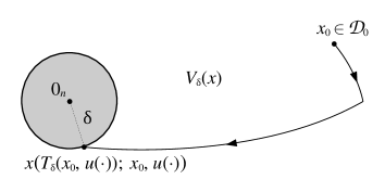
For numerical purposes, it is reasonable to approximate the infinite-horizon optimal control problem (47) by an exit-time problem. If a local CLF and its level sets are not practically obtained, the approach of Section 2 cannot be used. The exit-time problem is then stated with respect to the closed ball $\bar{\mathrm{B}}_{\delta}(0_{n})$ with center $x=0_{n}$ and sufficiently small radius $\delta\in(0,r]$ (see Fig. 2 and recall that the constant $r$ was introduced in Assumption 3.1):

(53) $$V_{\delta}(x_{0})\>\>\stackrel{{\scriptstyle\mathrm{def}}}{{=}}\>\>\inf\>\left\{\int\limits_{0}^{T}g(x(t;\,x_{0},u(\cdot)),\>u(t))\>\mathrm{d}t\>\,\colon\right.$$

$$\qquad\qquad\qquad\quad\left.u(\cdot)\in\mathcal{U},\>\,\,x(T;\,x_{0},u(\cdot))\>\in\>\bar{\mathrm{B}}_{\delta}(0_{n})\>\,\,\mbox{at some $\,T\in[0,+\infty)$}\right\}$$

$$\forall x_{0}\in G\quad\forall\delta\in(0,r].$$

The convention $\,\inf\,\emptyset=+\infty\,$ is adopted as before. With the help of the notation

(54) $$T_{\delta}(x_{0},u(\cdot))\>\>\stackrel{{\scriptstyle\mathrm{def}}}{{=}}\>\>\inf\,\left\{T\in[0,+\infty)\>\colon\>x(T;\,x_{0},u(\cdot))\>\in\>\bar{\mathrm{B}}_{\delta}(0_{n})\right\}\quad\forall x_{0}\in G\quad\forall u(\cdot)\in\mathcal{U}$$

for the exit times, the value function (53) can also be determined by

(55) $$V_{\delta}(x_{0})\>\>=\>\>\inf_{\begin{subarray}{c}u(\cdot)\,\in\,\mathcal{U}\>\colon\\ T_{\delta}(x_{0},\,u(\cdot))\><\>+\infty\end{subarray}}\>\left\{\int\limits_{0}^{T_{\delta}(x_{0},\,u(\cdot))}g(x(t;\,x_{0},u(\cdot)),\>u(t))\>\mathrm{d}t\right\}\quad\forall x_{0}\in G\quad\forall\delta\in(0,r]$$

(note that the running cost is nonnegative according to Item 1 of Assumption 3.5). Consider also the Kruzhkov transformed function

(56) $$v_{\delta}(x_{0})\>\,\stackrel{{\scriptstyle\mathrm{def}}}{{=}}\>\,1\,-\,e^{-V_{\delta}(x_{0})}\>\,\in\>\,[0,1]\quad\forall x_{0}\in G\quad\forall\delta\in(0,r].$$

Figure 2: The exit-time optimal control problem (53) (or, equivalently, (55)), whose target set is the closed ball with center $x=0_{n}$ and sufficiently small radius $\delta\in(0,r]$.

A key result on approximating the infinite-horizon problem (47) by the exit-time problem (53) (or, equivalently, by (55)) can now be derived.

Theorem 3.9.

Under Assumptions 2.1, 3.1 and 3.5, the following properties hold:

• the domain of asymptotic null-controllability can be represented as

  $$\mathcal{D}_{0}\>\>=\>\>\{x_{0}\in G\>\colon\>V_{\delta}(x_{0})\,<\,+\infty\}\>\>=\>\>\{x_{0}\in G\>\colon\>v_{\delta}(x_{0})\,<\,1\}\quad\forall\delta\in[0,r]$$

  (according to Definition 2.4, it is obvious that $\mathcal{D}_{0}$ does not depend on $\delta$);

• $v_{\delta}(x_{0})\to v_{0}(x_{0})\,$ uniformly on $G$ as $\delta\to+0$;

• $V_{\delta}(x_{0})\to V_{0}(x_{0})\,$ uniformly on every compact subset of $\mathcal{D}_{0}$ as $\delta\to+0$;

• for every $\delta\in(0,r]$, $V_{\delta}(\cdot)$ is locally Lipschitz continuous in $\mathcal{D}_{0}$ (and therefore differentiable almost everywhere in $\mathcal{D}_{0}$ with respect to the Lebesgue measure in $\mathbb{R}^{n}$) if the Petrov condition

  $$\min_{u\,\in\,U}\>\left<x,\,f(x,u)\right>\><\>0\quad\forall\>x\>\in\>\partial\mathrm{B}_{\delta}(0_{n})\>=\>\{x^{\prime}\in\mathbb{R}^{n}\>\colon\>\|x^{\prime}\|=\delta\}$$

  holds.

Proof.

For any $\delta\in(0,r]$, the condition $\,x_{0}\,\in\,G\setminus\mathcal{D}_{0}\,$ yields the absence of state trajectories $\>x(\cdot;\,x_{0},u(\cdot))\>$ corresponding to $u(\cdot)\in\mathcal{U}$ and reaching the target ball $\,\bar{B}_{\delta}(0_{n})\subseteq\bar{B}_{r}(0_{n})\,$ in finite time, while such trajectories exist if $x_{0}\in\mathcal{D}_{0}$ (recall Definition 2.4, Assumption 3.1, and the inclusion $\,\bar{\mathrm{B}}_{r}(0_{n})\subset\mathcal{D}_{0}\,$ from Proposition 3.4). This and the property (49) lead to Item 1.

Note that Item 3 would follow from Item 2, because

$$V_{\delta}(x_{0})\>=\>-\ln\,(1\,-\,v_{\delta}(x_{0}))\quad\forall x_{0}\in\mathcal{D}_{0}\quad\forall\delta\in[0,r]$$

by virtue of the relations (48), (49) and (56). Besides, Item 4 can be established similarly to Item 1 of Proposition 2.19 and the last sentence in Theorem 2.20.

It hence remains to verify Item 2. If $\,x_{0}\,\in\,G\setminus\mathcal{D}_{0},\,$ the statement follows directly from Item 1 and the representation (49). Now consider arbitrary $x_{0}\in\mathcal{D}_{0}$ and $\delta\in(0,r]$. Then the set of control strategies $u(\cdot)\in\mathcal{U}$ satisfying $\,T_{\delta}(x_{0},u(\cdot))<+\infty\,$ is nonempty. Due to Proposition 3.7, one has

(57) $$v_{0}(x_{0})\>\>=\>\>\inf\limits_{\begin{subarray}{c}u(\cdot)\,\in\,\mathcal{U}\>\colon\\ T_{\delta}(x_{0},\,u(\cdot))\><\>+\infty\end{subarray}}\>\left\{1\>\,-\>\,\mu\left(x_{0},\,u(\cdot),\,T_{\delta}(x_{0},u(\cdot))\right)\right.$$

$$\qquad\qquad\quad\left.+\>\,\mu\left(x_{0},\,u(\cdot),\,T_{\delta}(x_{0},u(\cdot))\right)\>\cdot\>v_{0}\left(x\left(T_{\delta}(x_{0},u(\cdot));\>x_{0},u(\cdot)\right)\right)\right\}.$$

By using the nonnegativity of the running cost, as well as the formulas (51), (55) and (56), one arrives at

(58) $$\begin{array}[]{c}0\><\>\mu(x_{0},u(\cdot),T)\>\leqslant\>1\quad\forall u(\cdot)\in\mathcal{U}\quad\forall T\geqslant 0,\\ v_{\delta}(x_{0})\>\>=\>\>\inf\limits_{\begin{subarray}{c}u(\cdot)\,\in\,\mathcal{U}\>\colon\\ T_{\delta}(x_{0},\,u(\cdot))\><\>+\infty\end{subarray}}\>\left\{1\>\,-\>\,\mu\left(x_{0},\,u(\cdot),\,T_{\delta}(x_{0},u(\cdot))\right)\right\}.\end{array}$$

Next, the obtained relations (57), (58) lead to

$$0 \leqslant\>\>v_{0}(x_{0})\>-\>v_{\delta}(x_{0})$$

$$\leqslant\>\>\sup\limits_{\begin{subarray}{c}u(\cdot)\,\in\,\mathcal{U}\>\colon\\ T_{\delta}(x_{0},\,u(\cdot))\><\>+\infty\end{subarray}}\>\left\{\mu\left(x_{0},\,u(\cdot),\,T_{\delta}(x_{0},u(\cdot))\right)\>\cdot\>v_{0}\left(x\left(T_{\delta}(x_{0},u(\cdot));\>x_{0},u(\cdot)\right)\right)\right\}$$

$$\leqslant\>\>\sup\limits_{\begin{subarray}{c}u(\cdot)\,\in\,\mathcal{U}\>\colon\\ T_{\delta}(x_{0},\,u(\cdot))\><\>+\infty\end{subarray}}\>v_{0}\left(x\left(T_{\delta}(x_{0},u(\cdot));\>x_{0},u(\cdot)\right)\right)$$

$$\leqslant\>\>\max\limits_{y\,\in\,\bar{\mathrm{B}}_{\delta}(0_{n})}\,v_{0}(y).$$

In order to complete the proof, it now suffices to use the property

$$\lim\limits_{\delta\,\to\,+0}\>\max\limits_{y\,\in\,\bar{\mathrm{B}}_{\delta}(0_{n})}\,v_{0}(y)\>\,=\>\,0,$$

which follows from the equality $v_{0}(0_{n})=0$ and the continuity of $v_{0}(\cdot)$ on $G$ mentioned in Theorem 3.6. ∎

Remark 3.10.

In contrast with the global CLF characterization in Theorem 2.20 involving a local CLF, the approximating value function $V_{\delta}(\cdot)$ for a fixed sufficiently small $\delta\in(0,r]$ leads to the so-called practical stabilization in $\mathcal{D}_{0}$ (see, e. g., [5, Subsection 2.11]), but not to the asymptotic one. Indeed, the exit-time optimal control problem (53) is stated without using a local CLF and therefore does not allow to obtain stabilizing control actions in the target ball $\bar{\mathrm{B}}_{\delta}(0_{n})$. ∎

In order to ensure the existence of optimal control strategies and to use Pontryagin’s principle for the exit-time problem (53) with $\,x_{0}\,\in\,\mathcal{D}_{0}\setminus\bar{\mathrm{B}}_{\delta}(0_{n})\,$ and $\delta\in(0,r]$, we also need Assumptions 2.21 and 2.23. Note that the case when $\,x_{0}\in\bar{\mathrm{B}}_{\delta}(0_{n})\,$ with $\delta\in(0,r]$ is trivial and yields $\>T_{\delta}(x_{0},u(\cdot))\,=\,0\>$ for all $u(\cdot)\in\mathcal{U}$.

The existence result can be verified similarly to Theorem 2.24.

Theorem 3.11.

Let Assumptions 2.1, 3.1, 3.5 and 2.21 hold. For any fixed initial state $\,x_{0}\,\in\,\mathcal{D}_{0}\setminus\bar{\mathrm{B}}_{\delta}(0_{n})\,$ and parameter $\delta\in(0,r]$, there exists an optimal control strategy for the exit-time problem (53) or, equivalently, for (55).

Remark 3.12.

Under Assumptions 2.1, 3.1, 3.5, 2.21 and 2.23, Pontryagin’s principle for the exit-time problem (53) with a fixed initial state $\,x_{0}\,\in\,\mathcal{D}_{0}\setminus\bar{\mathrm{B}}_{\delta}(0_{n})\,$ and a fixed parameter $\delta\in(0,r]$ can be formulated similarly to Theorem 2.25, but with the difference that now the terminal set appears as the ball $\bar{\mathrm{B}}_{\delta}(0_{n})$ and can be reduced to the sphere $\partial\mathrm{B}_{\delta}(0_{n})$, while the terminal cost vanishes. One should consequently have

$$\begin{array}[]{c}T^{*}\,=\,T_{\delta}(x_{0},u^{*}(\cdot)),\quad\|x^{*}(T^{*})\|\,=\,\delta,\\ p^{*}(T^{*})\>\,\in\>\,\mathrm{N}(x^{*}(T^{*});\,\bar{\mathrm{B}}_{\delta}(0_{n}))\>\,=\>\,\{\varkappa\,x^{*}(T^{*})\>\colon\>\varkappa\geqslant 0\}\end{array}$$

in the modified characteristic boundary value problem. ∎

The following characteristics based representation is established similarly to Theorem 2.28. For the Hamiltonian and set-valued extremal control map, the notations (32) and (37) are still used.

Theorem 3.13.

Let Assumptions 2.1, 3.1, 3.5, 2.21 and 2.23 hold. For any initial state $\,x_{0}\,\in\,\mathcal{D}_{0}\setminus\bar{\mathrm{B}}_{\delta}(0_{n})\,$ and parameter $\delta\in(0,r]$, the Kruzhkov transformed value $v_{\delta}(x_{0})$ defined by (53)–(56) is the minimum of

$$1\>\>-\>\>\exp\left\{-\int\limits_{0}^{T_{\delta}(x_{0},\,u^{*}(\cdot))}g(x^{*}(t),\,u^{*}(t))\>\mathrm{d}t\right\}$$

over the solutions of the characteristic Cauchy problems

$$\left\{\begin{aligned} &\dot{x^{*}}(t)\>\>=\>\>\mathrm{D}_{p}H(x^{*}(t),\,u^{*}(t),\,p^{*}(t),\,\tilde{p}^{*})\>\>=\>\>f(x^{*}(t),\,u^{*}(t)),\\ &\dot{p^{*}}(t)\>\>=\>\>-\mathrm{D}_{x}H(x^{*}(t),\,u^{*}(t),\,p^{*}(t),\,\tilde{p}^{*})\\ &\qquad\>\>=\>\>-(\mathrm{D}_{x}f(x^{*}(t),\,u^{*}(t)))^{\top}\>p^{*}(t)\>\,-\>\,\tilde{p}^{*}\>\mathrm{D}_{x}g(x^{*}(t),\,u^{*}(t)),\\ &u^{*}(t)\>\in\>U^{*}(x^{*}(t),\,p^{*}(t),\,\tilde{p}^{*}),\\ &t\>\,\in\>\,\begin{cases}[0,\,T_{\delta}(x_{0},\,u^{*}(\cdot))],&T_{\delta}(x_{0},\,u^{*}(\cdot))\><\>+\infty,\\ [0,+\infty),&T_{\delta}(x_{0},\,u^{*}(\cdot))\>=\>+\infty,\end{cases}\\ &x^{*}(0)\,=\,x_{0},\quad p^{*}(0)\,=\,p_{0},\end{aligned}\right.$$

for all extended initial adjoint vectors

$$(p_{0},\tilde{p}^{*})\>\,\in\>\,\{(p,\tilde{p})\>\colon\>p\in\mathbb{R}^{n},\>\>\tilde{p}\in\{0,1\}\}.$$

Moreover, the same value is obtained when minimizing over the bounded set

$$(p_{0},\tilde{p}^{*})\>\,\in\>\,\{(p,\tilde{p})\>\in\>\mathbb{R}^{n}\times\mathbb{R}\>\colon\>\|(p,\tilde{p})\|\>=\>1,\>\>\,\tilde{p}\geqslant 0\},$$

or even over its subset

$$(p_{0},\tilde{p}^{*})\>\,\in\>\,\{(p,\tilde{p})\>\in\>\mathbb{R}^{n}\times\mathbb{R}\>\colon\>\|(p,\tilde{p})\|\>=\>1,\>\>\,\tilde{p}\geqslant 0,\>\>\,\mathcal{H}(x_{0},p,\tilde{p})\>=\>0\}.$$

Theorems 3.6, 3.9, 3.11, 3.13 together with Remarks 3.10, 3.12 constitute the theoretical foundation of a curse-of-dimensionality-free approach to approximating CLFs and feedback stabilization in case when one does find an appropriate local CLF.

4 A curse-of-dimensionality-free approach to CLF approximation and feedback stabilization

In the introduction, several well-known grid based numerical methods for solving Hamilton–Jacobi equations and constructing optimal feedback strategies were noted. They typically require dense state space discretizations and may face the practical dilemma of selecting a suitable bounded region for computations (in order to reduce boundary cutoff errors in a relevant subdomain).

Alternatively, one can use the results of Sections 2 and 3 in order to approximate CLFs and associated feedbacks independently at different initial states. As was discussed in the introduction, this enables for attenuating the curse of dimensionality and selecting arbitrary bounded regions and grids in the state space. Parallel computations can also be arranged.

Furthermore, the stabilizing control action at any isolated state can be directly retrieved either as the initial value of an approximate optimal open-loop control strategy computed via a direct method, or by the corresponding representation in Pontryagin’s principle (recall (37)) with the initial state and an approximate optimal initial costate. The latter can be obtained via an indirect characteristics based method or as an appropriate costate estimate building on direct collocation [50, 51]. Possibly unstable approximations of the gradient of the CLF are therefore not needed.

As was also noted in the introduction, even if the curse of dimensionality is mitigated, the curse of complexity is still a formidable issue when constructing global or semi-global solution approximations in high-dimensional regions. Sparse grid frameworks (see, e. g., [35, 70] and [71, §3.7]) may help to attenuate that if the dimension is not too high (typically not greater than $6$) and if the sought-after functions are smooth enough. However, the range of applicability of sparse grids to solving feedback control problems has to be further investigated.

More details and recommendations on implementing the curse-of-dimensionality-free approach are given in Section A.2 of Online_App the appendix. They focus on the setting of Section 2 with a local CLF involved. Similar practical considerations excluding local CLF construction can be applied to the setting of Section 3. However, further development of efficient numerical algorithms with software implementations is left for future research.

Subsection A.2.1 of Online_App the appendix describes a linearization based numerical technique for building quadratic local CLFs under some additional conditions, with the considerations of [53, Section 3] serving as an important motivation. Those considerations can also be employed for constructing quadratic local CLFs under the same assumptions. Although the technique presented in Online_App the appendix is less elegant and may be more computationally expensive, it is more straightforward to use and does not restrict the right-hand sides in the decrease conditions for the resulting local CLFs necessarily to quadratic functions (in contrast to the approach of [53, Section 3]).

In Online_App the appendix, Subsection A.2.2 develops a numerical framework using the characteristics based representation in Theorem 2.28, Subsection A.2.3 briefly discusses the use of direct approximation methods, and, finally, Subsection A.2.4 points out how our curse-of-dimensionality-free approach can be incorporated in model predictive control schemes and how sparse grids may be involved.

5 Numerical simulations

In this section, we consider two examples for testing certain implementaions of the discussed curse-of-dimensionality-free approach to CLF approximation and feedback stabilization. The first example involves a nonlinear control system with two-dimensional state space and can be treated analytically to some extent, so that the exact and numerical solutions can be compared with each other. In the second example, a model predictive control scheme (see Subsection A.2.4 in Online_App the appendix) incorporating that approach is applied to an essentially more complicated nonlinear control system with six-dimensional state space.

The numerical simulations were conducted on a relatively weak machine with 1.4 GHz Intel 2957U CPU, and no parallel programming tools were used. The runtimes can be significantly shorter for more powerful machines, especially when parallelization is done.

Example 5.1.

Consider the control system (1) with $\>n=2$, $\,m=1$, $\,x=(x_{1},x_{2})^{\top}\in\mathbb{R}^{2}$, $\,x(0)=x^{0}\in\mathbb{R}^{2}$, $\,G=\mathbb{R}^{2}$, $\,U\subseteq\mathbb{R},\>$ and

(59) $$f(x,u)\>\,=\>\,\begin{pmatrix}x_{1}\,+\,2x_{2}\,+\,u\\ -x_{2}\,-\,2x_{1}^{3}\end{pmatrix}\quad\forall x\in\mathbb{R}^{2}\quad\forall u\in U$$

(see [72, Example 1.1]).

First, let $U=\mathbb{R}$. The proper, positive definite, and infinitely differentiable function

(60) $$\tilde{V}(x)\>\,\stackrel{{\scriptstyle\mathrm{def}}}{{=}}\>\,\frac{1}{4}\,x_{1}^{4}\>+\>\frac{1}{2}\,x_{2}^{2}\quad\forall x\in\mathbb{R}^{2}$$

is a global CLF for this system in the whole state space. Indeed,

$$\left<\mathrm{D}\tilde{V}(x),\,f(x,u)\right>\>\>=\>\>x_{1}^{3}\,(x_{1}\,+\,2x_{2}\,+\,u)\>+\>x_{2}\,\left(-x_{2}\,-\,2x_{1}^{3}\right)\>\>=\>\>x_{1}^{3}\,(x_{1}\,+\,u)\>-\>x_{2}^{2}$$

$$\forall x\in\mathbb{R}^{2}\quad\forall u\in\mathbb{R},$$

so that, for any constant $b>0$ and for any bounded continuous function $\,\chi\colon\mathbb{R}\to\mathbb{R}\,$ satisfying

(61) $$\chi(x_{1})\,\geqslant\,b\quad\forall x_{1}\in\mathbb{R},$$

the feedback control strategy

(62) $$\tilde{u}(x)\>\,\stackrel{{\scriptstyle\mathrm{def}}}{{=}}\>\,-(1\,+\,\chi(x_{1}))\>x_{1}\quad\forall x\in\mathbb{R}^{2}$$

is globally stabilizing due to

$$\left<\mathrm{D}\tilde{V}(x),\,f(x,\tilde{u}(x))\right>\>\>=\>\>-\chi(x_{1})\,x_{1}^{4}\>-\>x_{2}^{2}\>\>\leqslant\>\>-bx_{1}^{4}\>-\>x_{2}^{2}\quad\forall x\in\mathbb{R}^{2}.$$

Introduce also the running cost

(63) $$g(x,u)\>\,=\>\,2x_{1}^{4}\>+\>x_{2}^{2}\>+\>\frac{1}{256}\,u^{4}\quad\forall x\in\mathbb{R}^{2}\quad\forall u\in\mathbb{R}.$$

With the help of the classical verification result [6, Chapter VII, Theorem 2.2], one can show that (60) is the value function in the infinite-horizon optimal control problem

(64) $$\tilde{V}\left(x^{0}\right)\>\>=\>\>\min_{u(\cdot)\>\,\in\>\,L_{\mathrm{loc}}^{\infty}([0,+\infty),\>\mathbb{R})}\>\left\{\int\limits_{0}^{+\infty}g\left(x\left(t;\,x^{0},u(\cdot)\right),\>u(t)\right)\>\mathrm{d}t\right\}\quad\forall x^{0}\in\mathbb{R}^{2}$$

for the considered system and running cost, and that

(65) $$\tilde{u}^{*}(x)\,=\,-4x_{1}$$

is the corresponding optimal feedback control strategy.

Next, take the set of pointwise control constraints as the bounded line segment

(66) $$U\,=\,[-a,a]$$

with a constant $a>0$. Furthermore, fix a constant $b>0$ and a bounded continuous function $\,\chi\colon\mathbb{R}\to\mathbb{R}\,$ satisfying (61), and choose a constant $c>0$ such that the feedback strategy (62) fulfills

(67) $$\tilde{u}(x)\,\in\,U\,=\,[-a,a]\quad\forall x\in\Omega_{c}$$

in the sublevel set

(68) $$\Omega_{c}\>\,\stackrel{{\scriptstyle\mathrm{def}}}{{=}}\>\,\{x\in\Omega_{c}\>\colon\>\tilde{V}(x)\,\leqslant\,c\}$$

of $\tilde{V}(\cdot)$. Hence, the restrictions of $\tilde{V}(\cdot)$ and $\tilde{u}(\cdot)$ to $\Omega_{c}$ are a local CLF and a locally stabilizing feedback, respectively. Besides, there exists a constant $c^{*}>0$ such that the restriction of $\tilde{u}^{*}(\cdot)$ to $\Omega_{c^{*}}$ is also a locally stabilizing feedback. For convenience, denote

(69) $$V_{\mathrm{loc}}(x)\,\stackrel{{\scriptstyle\mathrm{def}}}{{=}}\,\tilde{V}(x),\quad u_{\mathrm{loc}}(x)\,\stackrel{{\scriptstyle\mathrm{def}}}{{=}}\,\tilde{u}(x),\quad u^{*}_{\mathrm{loc}}(x)\,\stackrel{{\scriptstyle\mathrm{def}}}{{=}}\,\tilde{u}^{*}(x)\quad\forall x\in\mathbb{R}^{2}.$$

Now it is not difficult to check that Theorems 2.20, 2.24, 2.25, 2.27 and 2.28 can be used with the specified local CLF $V_{\mathrm{loc}}(\cdot)$, sublevel set $\Omega_{c}$, and running cost (63). In particular, a global CLF $V(\cdot)$ in $\mathcal{D}_{0}$ is determined by (21), (26), and its Kruzhkov transform is given by (36). Introduce also the Kruzhkov transform of $V_{\mathrm{loc}}(\cdot)$:

(70) $$v_{\mathrm{loc}}\left(x^{0}\right)\>\,\stackrel{{\scriptstyle\mathrm{def}}}{{=}}\>\,1\,-\,e^{-V_{\mathrm{loc}}\left(x^{0}\right)}\quad\forall x^{0}\in\mathbb{R}^{2}.$$

In order to approximate the global CLF and stabilizing feedback, as well as to construct a reasonable inner estimate for the domain of asymptotic null-controllability, the characteristics based framework of Subsection A.2.2 in Online_App the appendix was used. It is not difficult to verify the fulfillment of Assumptions A.2.3–A.2.5 from that subsection.

We take

(71) $$\begin{array}[]{c}a\,=\,1.2,\quad b\,=\,1.4,\quad c\,=\,0.015,\quad c_{1}\,=\,0.01,\quad T_{\max}\,=\,10,\\ \varepsilon\,=\,10^{-15},\quad\varepsilon_{1}\,=\,0.005,\quad\delta_{1}\,=\,0.005,\quad\delta_{2}\,=\,0.005\end{array}$$

(the notations $T_{\max},\varepsilon,\varepsilon_{1}$ and $c_{1},\delta_{1},\delta_{2}$ were introduced respectively in Subsections A.2.2.1 and A.2.2.2 of Online_App the appendix),

(72) $$\chi(x_{1})\>\,=\>\,\begin{cases}3,&-4x_{1}\,\in\,[-a,a],\\ \max\left\{\dfrac{a}{|x_{1}|}\,-\,1,\>\,b\right\},&-4x_{1}\,\notin\,[-a,a],\end{cases}$$

so that $\chi(\cdot)$ is bounded and continuous, (61) holds,

(73) $$\frac{a}{|x_{1}|}\>>\>1\,+\,b\quad\mbox{at all points~{}$\,x\in\Omega_{c}\,$ for which $x_{1}\neq 0$,}$$

and (62), (69), (72), (73) imply the following relations:

(74) $$u_{\mathrm{loc}}(x)\>\,=\>\,\tilde{u}(x)\>\,=\>\,\begin{cases}u^{*}_{\mathrm{loc}}(x)\,=\,\tilde{u}^{*}(x)\,=\,-4x_{1},&-4x_{1}\,\in\,[-a,a],\\ -x_{1}\>\max\left\{\dfrac{a}{|x_{1}|}\,,\>\,1+b\right\},&-4x_{1}\,\notin\,[-a,a],\end{cases}$$

$$u_{\mathrm{loc}}(x)\>=\>-a\,\,\mathrm{sign}\>x_{1}\quad\mbox{at all points~{}$\,x\in\Omega_{c}\,$ for which $\,-4x_{1}\,\notin\,[-a,a]$.}$$

For a stabilizing feedback $\,u^{*}\colon\mathcal{D}_{0}\to U\,$ related to the CLF $V(\cdot)$, we put

(75) $$u^{*}(x)\,=\,u_{\mathrm{loc}}(x)\quad\forall x\in\Omega_{c}.$$

The characteristic Cauchy problems (39) and (A.22) (see Theorem 2.28 as well as Subsection A.2.2.2 in Online_App the appendix) were numerically solved via the Dormand–Prince fifth-order Runge–Kutta algorithm from [71, Chapter 17]. When launching the related routine, the initial guess for the stepsize was specified as $2\cdot 10^{-4}$, and the absolute and relative tolerances were selected as $10^{-6}$. The output data was obtained for the uniform time grid on $[0,T_{\max}]$ with the stepsize $2\cdot 10^{-4}$. In particular, the shooting costs were approximated from the state trajectory discretizations on this time grid.

The initial states were chosen from the grid on the rectangle $\,[-2,2]\times[-2.5,2.5]\,$ with the spatial steps $0.0625$ and $0.1$ along $x_{1}$-axis and $x_{2}$-axis, respectively. For solving the main and auxiliary finite-dimensional optimization problems formulated in Theorem 2.28 and Subsection A.2.2.2 of Online_App the appendix, we used the Powell algorithm from [71, §10.7] (which does not require evaluation of derivatives), and the corresponding tolerances were set as $10^{-6}$ and $10^{-8}$, respectively. For each state $x^{0}$ on the selected rectangular grid, the Powell iterative process for the auxiliary shooting problem was run from $\>N_{\mbox{\scriptsize opt. init. guess}}\,=\,4\>$ initial guesses that were randomly generated according to the uniform distribution with respect to the angles in the unit sphere parametrization (see (A.32) in Online_App the appendix). The unique point (A.26) and the roots of the function (A.29) (see these formulas in Online_App the appendix) were computed via the bisection algorithm from [71, §9.1], and the tolerance was taken as $10^{-13}$. An upper bound for the sought-after root $\lambda$ in (A.26) was chosen as $0.5$ (since $\,\Omega_{c_{1}}\subset\mathrm{B}_{0.5}(0_{2})$). Possible multiple roots of the function (A.29) on $(0,1)$ were bracketed by using the zbrak routine from [71, §9.1]. The bracketing pairs were searched for after dividing the interval $[0,1]$ into $100$ equally spaced segments.

The tolerance for the practical verification of equalities and non-strict inequalities via strict inequalities was set as $10^{-15}$.

In the case when we could not find a characteristic reaching the target set $\Omega_{c}$ and generating a cost less than $1-\varepsilon$ for some initial state $x^{0}$ (this might be not only a node on the specified rectangular grid, but also a shooting estimate $\hat{x}^{0}$ as described in the end of Subsection A.2.2.2 in Online_App the appendix), the computation was rerun with the increased parameter values $\>T_{\max}\,=\,T_{\max,\>\mathrm{recomp.}}\,=\,20\>$ and $\>N_{\mbox{\scriptsize opt. init. guess}}\,=\,N_{\mbox{\scriptsize opt. init. guess, recomp.}}\,=\,5$. In such situations, the resulting data was taken from the second attempt ($v\left(x^{0}\right)$ might again be estimated as $1-\varepsilon$, which would indeed be reasonable if $x^{0}\notin\mathcal{D}_{0}$).

The related numerical simulation results are illustrated in Figs. 3–5.

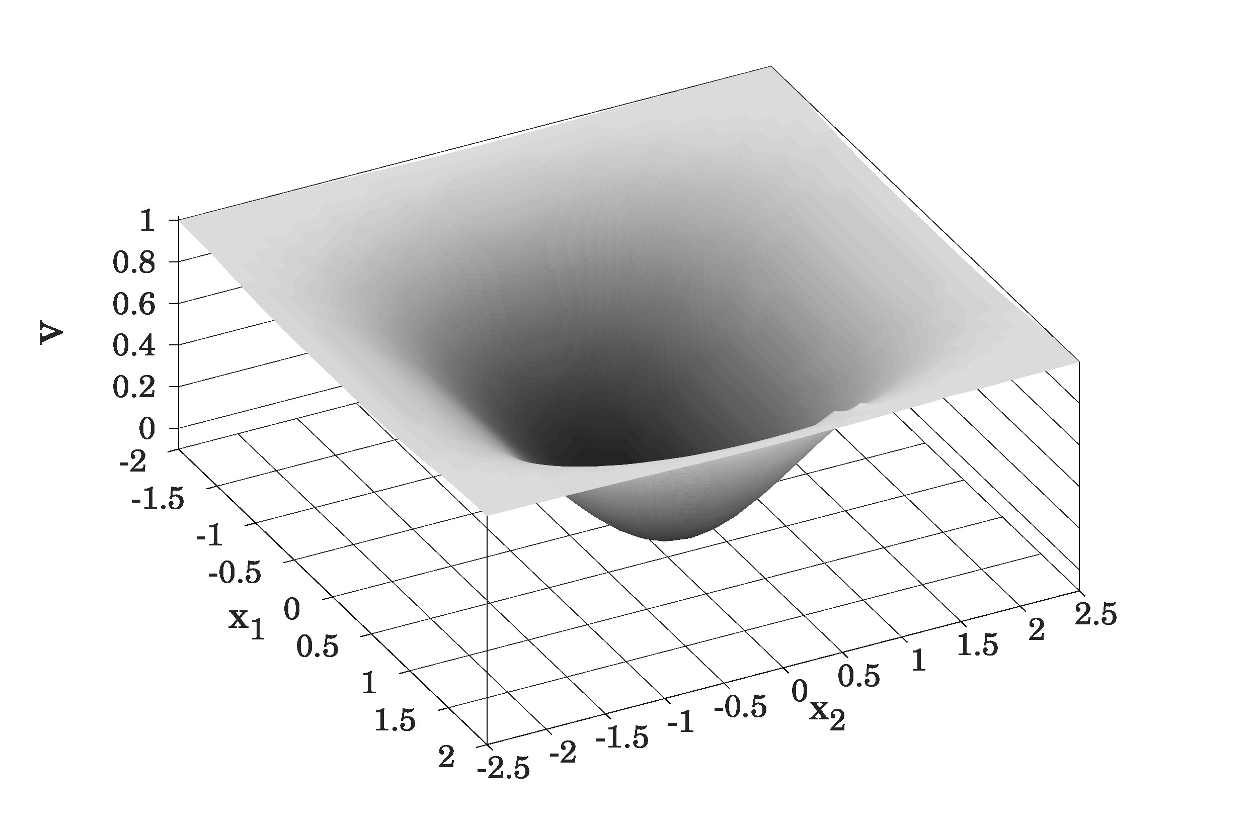
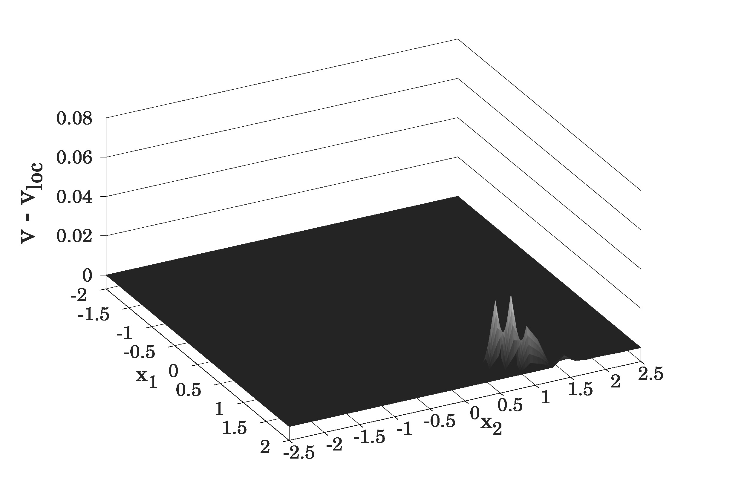
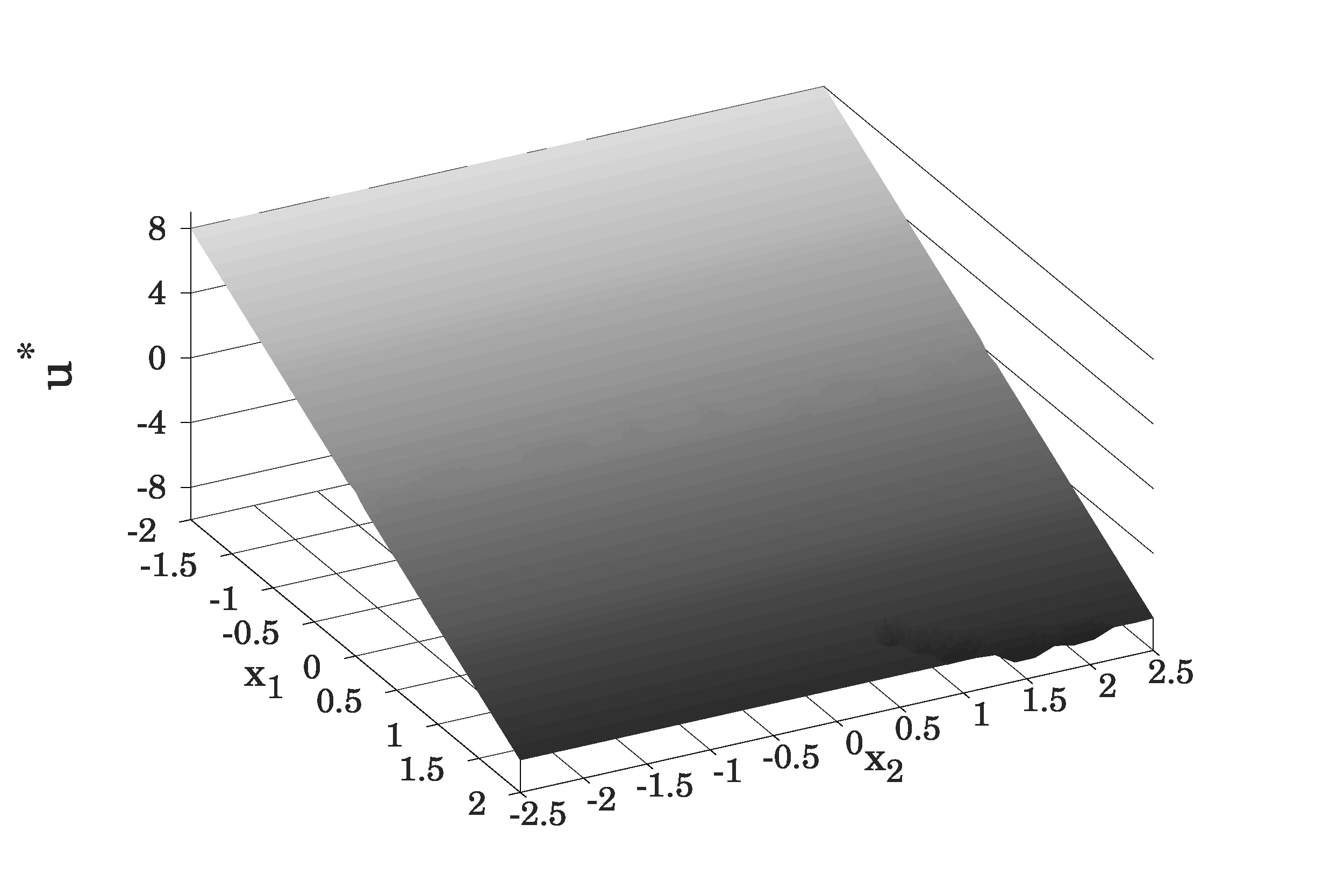
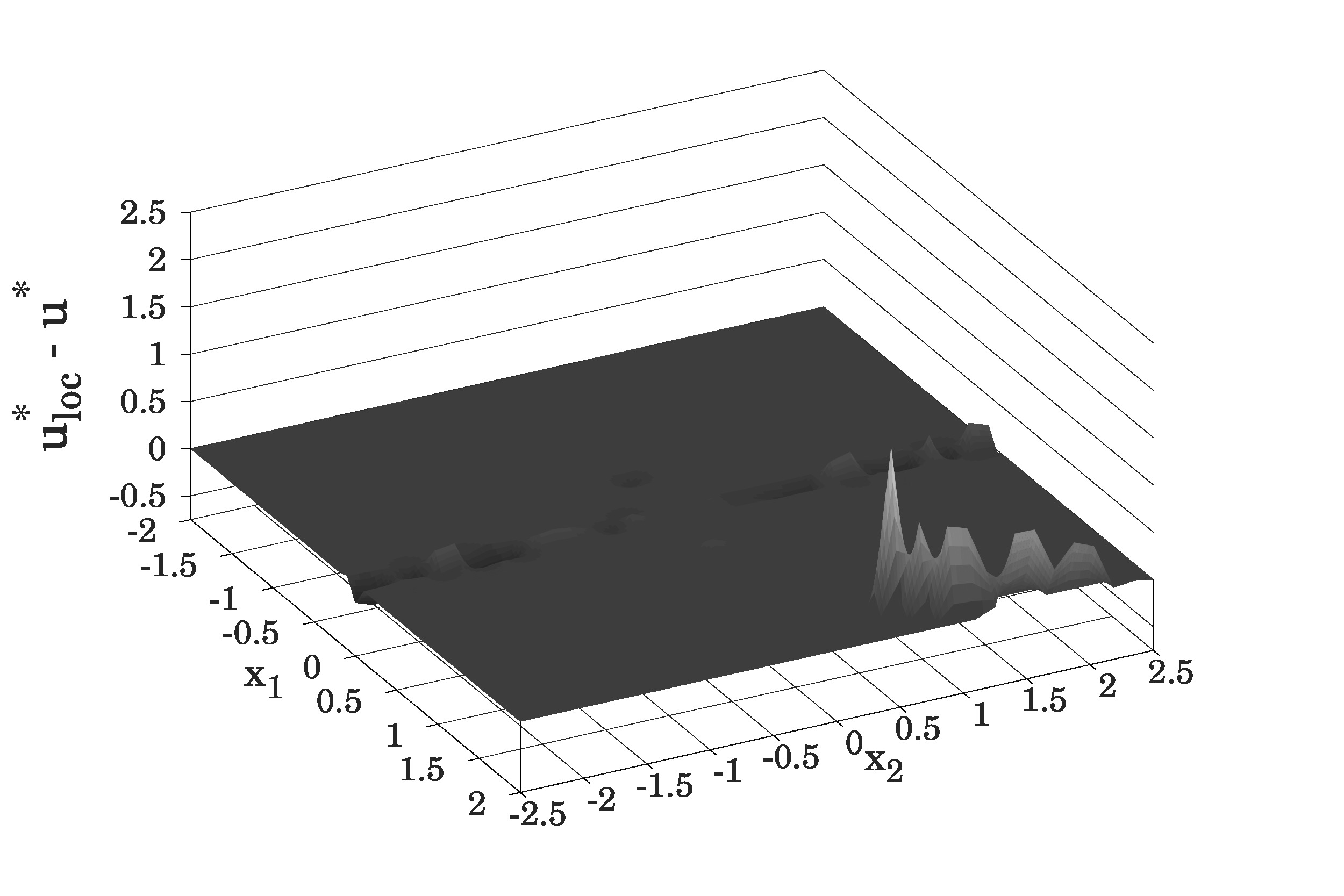
Fig. 3 indicates the Kruzhkov transformed functions $v(\cdot),v_{\mathrm{loc}}(\cdot)$ and their difference. Fig. 4 shows the corresponding feedback strategies $u^{*}(\cdot),u^{*}_{\mathrm{loc}}(\cdot)$ and their difference. In Fig. 3, some approximated level sets of $v(\cdot)$ are depicted as well. In particular, the level $\,v(x)=1-e^{-c}\,$ (or, equivalently, $V(x)=c$) describes the boundary $l_{c}=\partial\Omega_{c}$, while the level $\,v(x)=1-\varepsilon_{1}=0.995\,$ is selected to represent an inner estimate of the domain of asymptotic null-controllability $\mathcal{D}_{0}$. The illustrations agree with the reasonable expectation that $v(\cdot)$ and $v_{\mathrm{loc}}(\cdot)$ should coincide in some region strictly containing $\Omega_{c}$, and that $\,u^{*}(x)=u^{*}_{\mathrm{loc}}(x)\,$ for all $x$ lying in this region and satisfying $\,u^{*}_{\mathrm{loc}}(x)\in U=[-a,a]\,$ (due to (74) and (75), one also has $\,u^{*}(x)=u_{\mathrm{loc}}(x)\,$ for all such $x$ and everywhere in $\Omega_{c}$).

Figure 3: The Kruzhkov transformed functions $v(\cdot),v_{\mathrm{loc}}(\cdot)$ and their difference for $U=[-1.2,1.2]$ in Example 5.1. Some approximated level sets of $v(\cdot)$ are shown as well. In order to see the graph of the difference between $v(\cdot)$ and $v_{\mathrm{loc}}(\cdot)$ clearer, the scale of the vertical axis in the third subfigure is modified as compared to that in the first two subfigures.

Figure 4: The feedback control strategies $u^{*}(\cdot),u^{*}_{\mathrm{loc}}(\cdot)$ (corresponding to $v(\cdot),v_{\mathrm{loc}}(\cdot)$, respectively) and their difference for $U=[-1.2,1.2]$ in Example 5.1. In order to see the graphs clearer, we do not fix the same scale for the vertical axes in the subfigures.

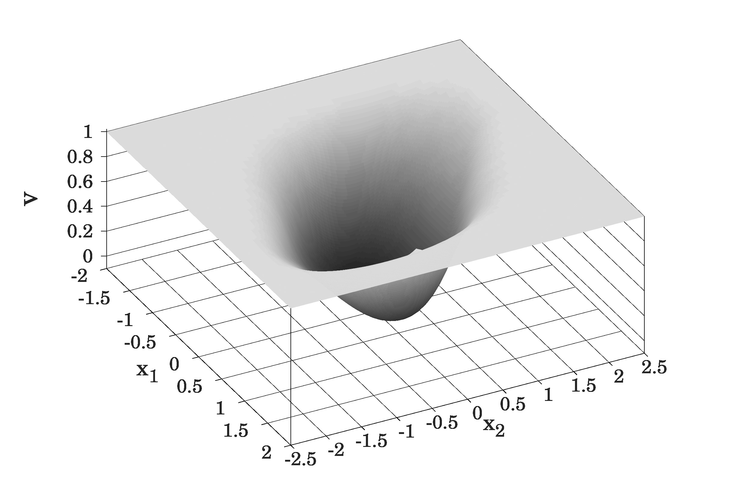
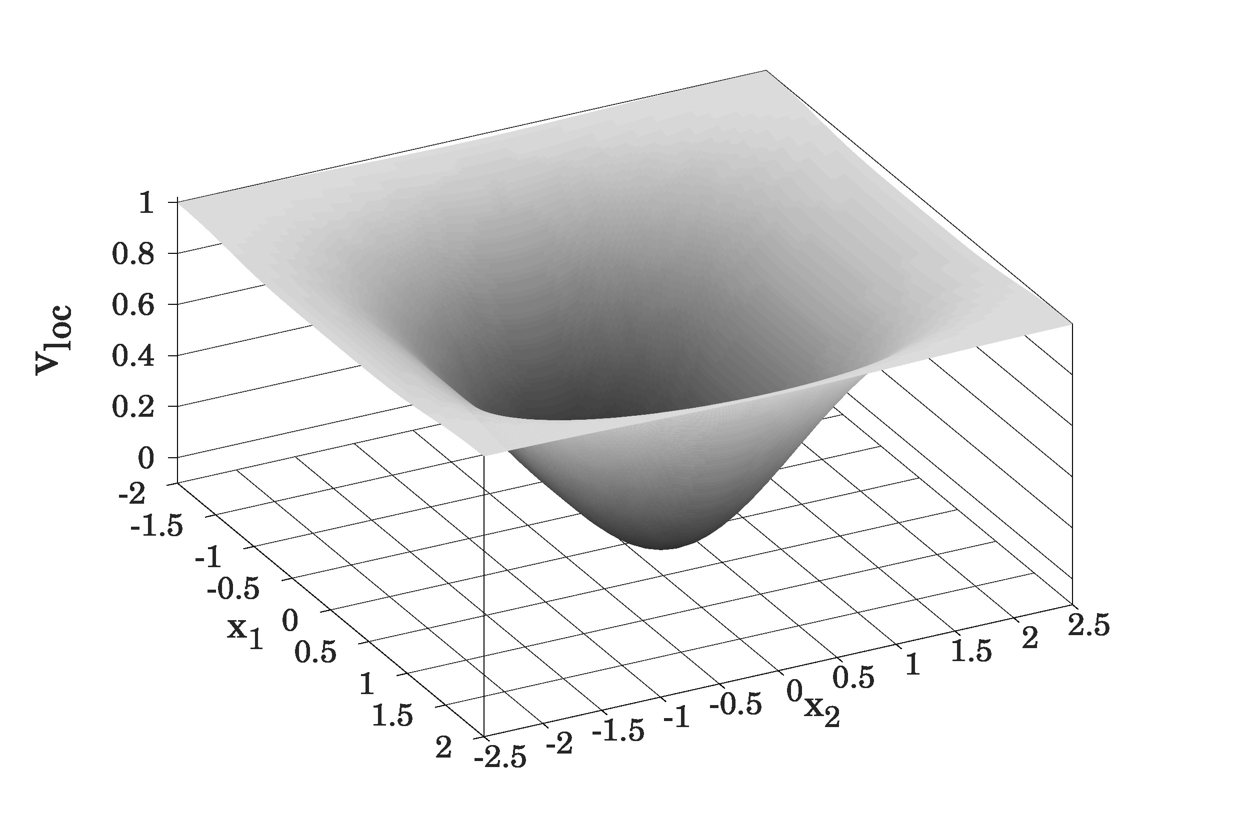
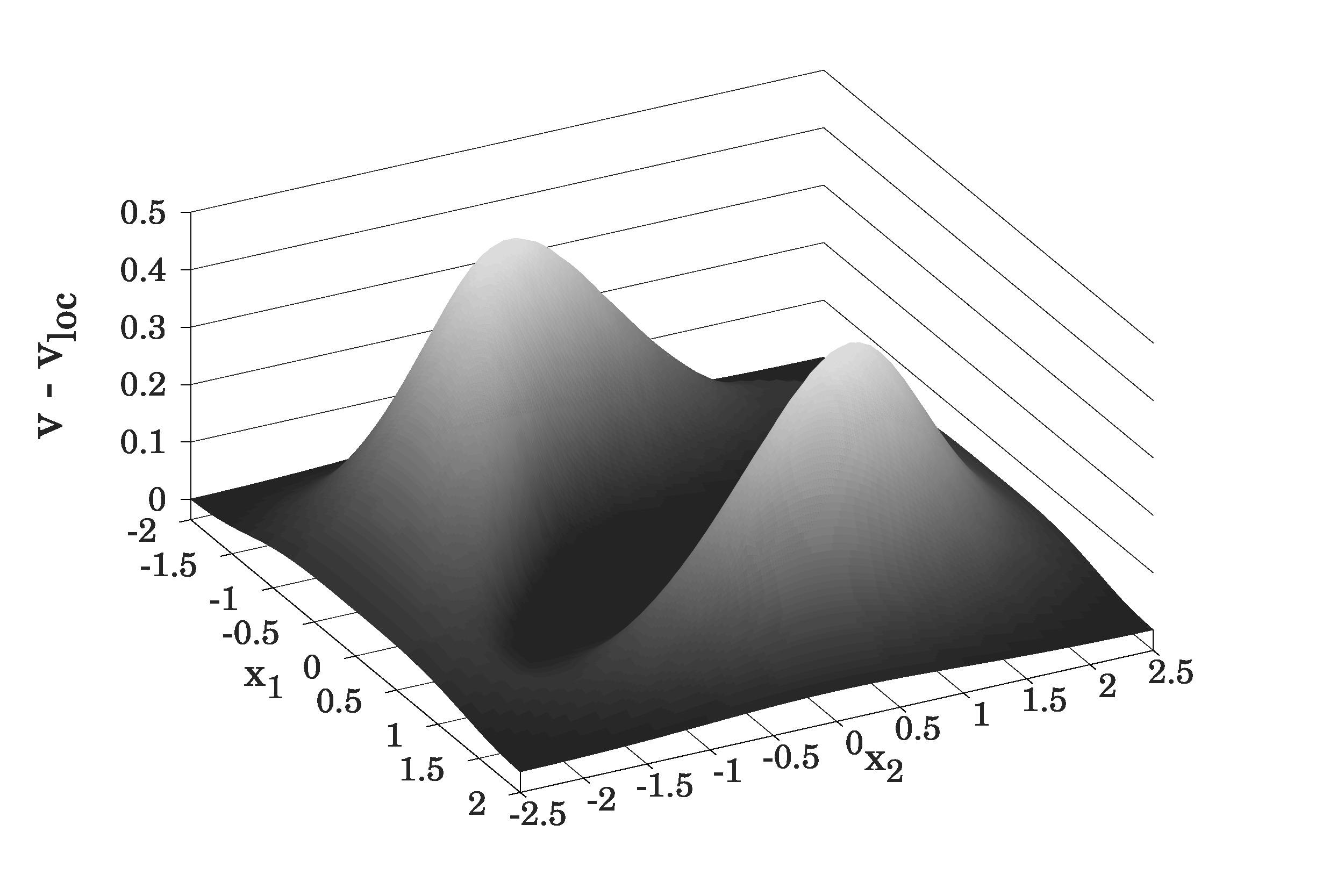
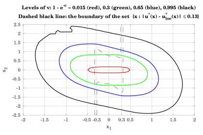
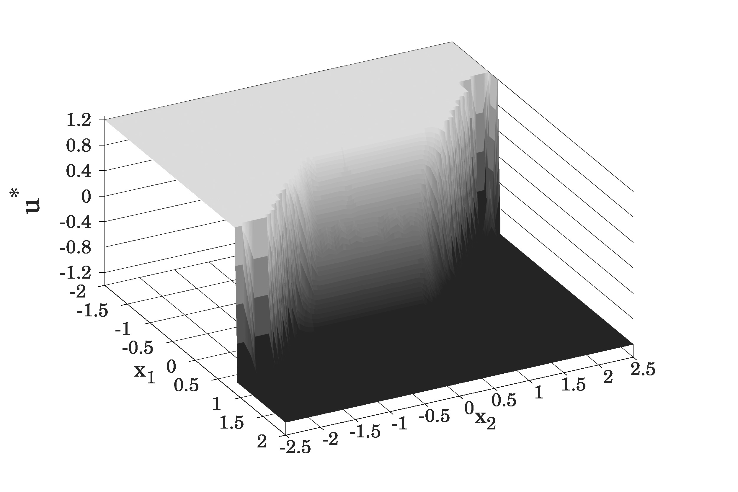
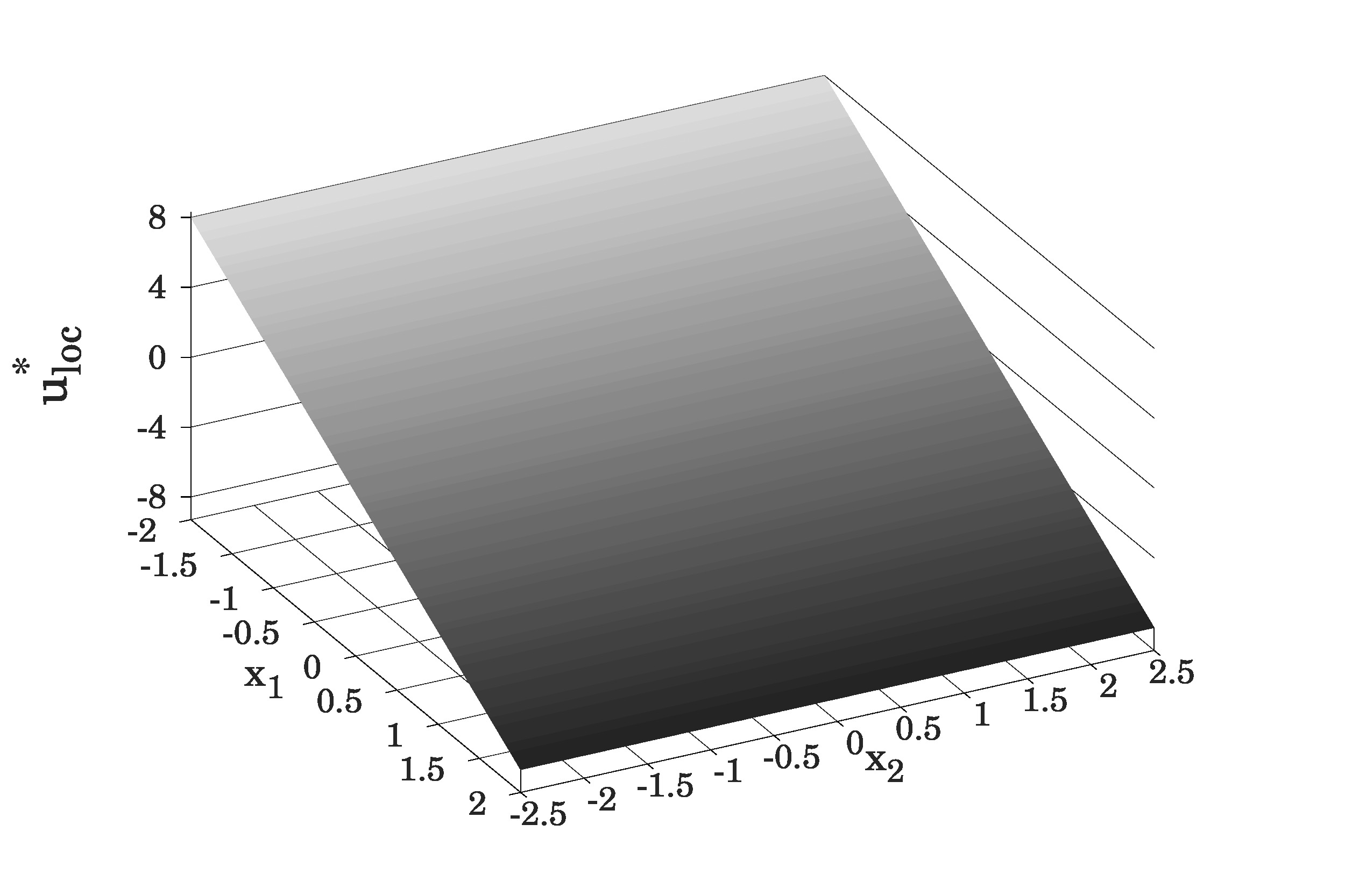
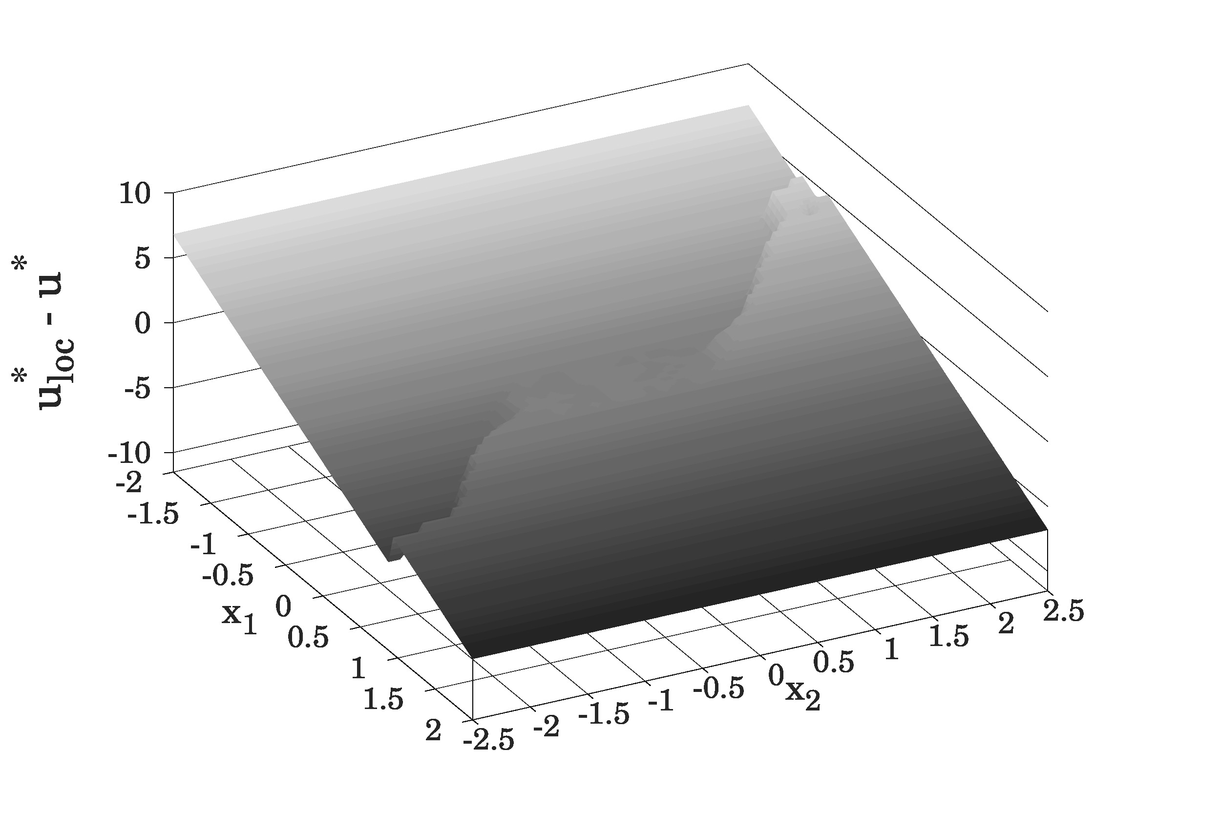
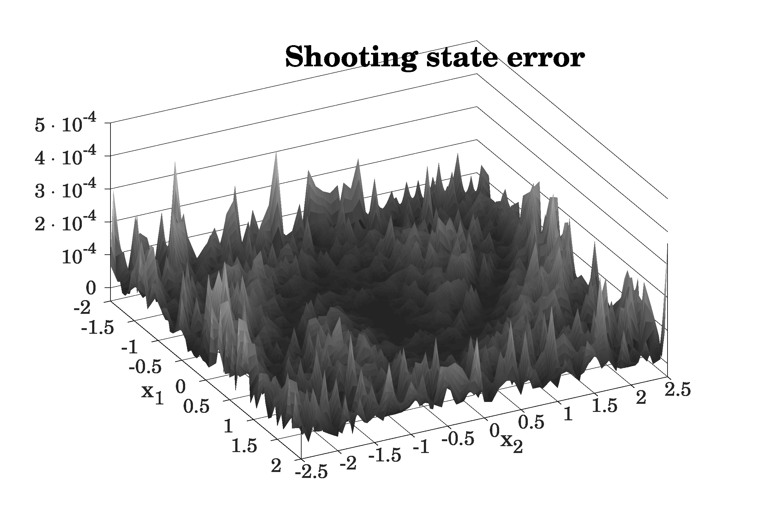
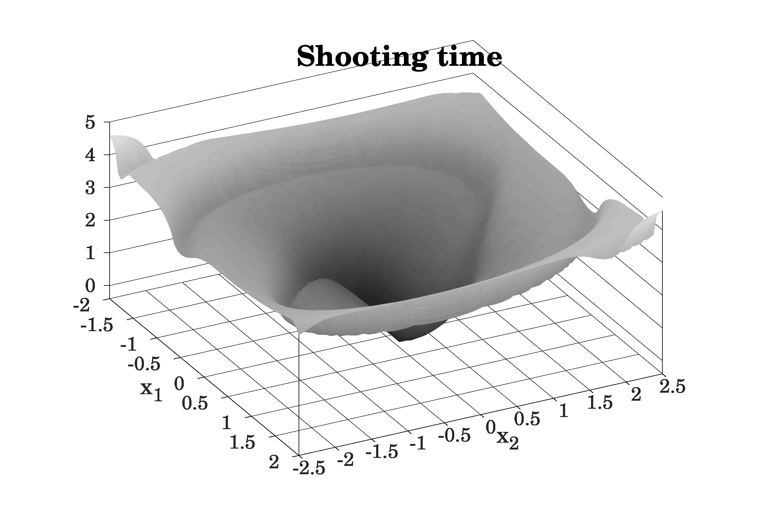
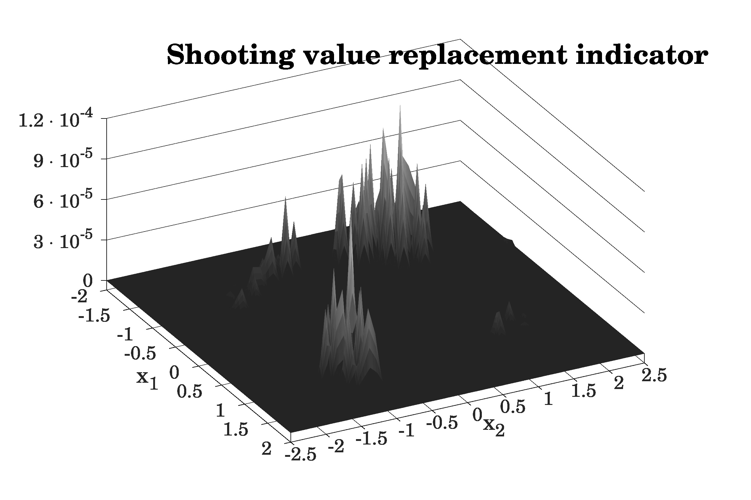
Fig. 5 shows the graphs of the following functions:

• the shooting state error defined as the square root of the numerical estimate of the minimum quadratic shooting cost (see Subsection A.2.2.2 in Online_App the appendix and note that, even when the exact minimum value of the lowest deviation (A.31) is zero, its approximation does not vanish for $x^{0}\notin\Omega_{c}$);

• the shooting time defined as an approximate minimizer in (A.31) for an optimal shooting reverse-time characteristic;

• the shooting value replacement indicator defined as zero if one arrives at a value less than $1-\varepsilon$ after one or two attempts to compute $v\left(x^{0}\right)$, and as the absolute difference $\,\left|v_{1}\left(x^{0}\right)-v\left(\hat{x}^{0}\right)\right|\,$ in the other case when one uses the first-order estimation technique proposed in the end of Subsection A.2.2.2.

The shooting state error and the shooting value replacement indicator on the considered grid are small enough to conjecture that the whole rectangle is contained in the domain of asymptotic null-controllability $\mathcal{D}_{0}$. However, rigorous verification of that for the selected bounded control constraint set $U=[-1.2,1.2]$ remains an open problem. Another open question is whether $\mathcal{D}_{0}$ is bounded for a bounded $U$ or not. Nevertheless, inner estimates of $\mathcal{D}_{0}$ obtained via our numerical approach may often suit practical needs.

Figure 5: The shooting state error, shooting time, and shooting value replacement indicator for $U=[-1.2,1.2]$ in Example 5.1. Different scales are used for the vertical axes in the subfigures.

In order to practically check the obvious fact that, for a sufficiently large $a$ and $U=[-a,a]$, the functions $v(\cdot)$ and $u^{*}(\cdot)$ should coincide in the considered bounded rectangle with $v_{\mathrm{loc}}(\cdot)$ and $u^{*}_{\mathrm{loc}}(\cdot)$, respectively, we performed numerical simulations for the increased parameter value $a=20$. We also reduced $T_{\max}$ from $10$ to $5$. Moreover, the spatial steps along $x_{1}$-axis and $x_{2}$-axis for the grid on the rectangle $\,[-2,2]\times[-2.5,2.5]\,$ were increased to $0.1$ and $0.15625$, respectively. All other parameters kept their values (in particular, $\>T_{\max,\>\mathrm{recomp.}}\,=\,20\>$ remained the same). The results are illustrated in Fig. 6.

Figure 6: The Kruzhkov transformed function $v(\cdot)$, the difference between $v(\cdot)$ and $v_{\mathrm{loc}}(\cdot)$, the feedback control strategy $u^{*}(\cdot)$, and the difference between $u^{*}_{\mathrm{loc}}(\cdot)$ and $u^{*}(\cdot)$ for $U=[-20,20]$ in Example 5.1. In order to see the graphs clearer, we do not fix the same scale for the vertical axes in the subfigures.

The average runtime per one initial state was around 18 seconds when obtaining the data for Figs. 3–5 and around 11 seconds when obtaining the data for Fig. 6. Such relatively long runtimes can be explained as follows. First, we used a rather weak machine, as was already noted in the beginning of this section. Second, our rectangle in the state space was large enough for constructing a reasonable inner estimate of $\mathcal{D}_{0}$, and the runtimes for the grid nodes not very far from $\Omega_{c}$ were much shorter than the average runtime (for $x^{0}\in\Omega_{c}$, we put $\>V\left(x^{0}\right)=V_{\mathrm{loc}}\left(x^{0}\right)$, $\,u^{*}\left(x^{0}\right)=u_{\mathrm{loc}}\left(x^{0}\right)\>$ and did not even need to optimize). ∎

Example 5.2.

The dynamics of a planar vertical takeoff and landing (PVTOL) aircraft can be described by the control system [7, 73, 74, 75]

(76) $$\left\{\begin{aligned} &\dot{x}_{1}(t)\>\>=\>\>x_{2}(t),\\ &\dot{x}_{2}(t)\>\>=\>\>-(1+u_{1}(t))\,\sin\,x_{5}(t)\,\,+\,\,\alpha\,u_{2}(t)\,\cos\,x_{5}(t),\\ &\dot{x}_{3}(t)\>\>=\>\>x_{4}(t),\\ &\dot{x}_{4}(t)\>\>=\>\>(1+u_{1}(t))\,\cos\,x_{5}(t)\,\,+\,\,\alpha\,u_{2}(t)\,\sin\,x_{5}(t)\,\,-\,\,1,\\ &\dot{x}_{5}(t)\>\>=\>\>x_{6}(t),\\ &\dot{x}_{6}(t)\>\>=\>\>u_{2}(t),\\ &t\geqslant 0,\\ &x\>=\>(x_{1},x_{2},x_{3},x_{4},x_{5},x_{6})^{\top},\quad u\>=\>(u_{1},u_{2})^{\top},\quad n=6,\quad m=2,\\ &x(0)\,=\,x^{0}\,\in\,G\,=\,\mathbb{R}^{6},\\ &u(\cdot)\>\in\>\mathcal{U}\>\stackrel{{\scriptstyle\mathrm{def}}}{{=}}\>L^{\infty}_{\mathrm{loc}}([0,+\infty),\,U),\quad U\subseteq\mathbb{R}^{2},\end{aligned}\right.$$

where the following notation is used (see Fig. 7):

• $t$ is a time variable;

• $x_{1}$ and $x_{3}$ are normalized quantities that correspond to the horizontal and vertical coordinates of the center of mass of the aircraft in a fixed inertial frame;

• $x_{5}$ is the roll angle that the aircraft makes with the positive horizontal axis;

• $x_{2}$, $x_{4}$, and $x_{6}$ are the rates of change of $x_{1}$, $x_{3}$, and $x_{5}$, respectively;

• $u_{1}$ and $u_{2}$ are normalized control inputs such that $1+u_{1}$ corresponds to the thrust (directed out the bottom of the aircraft), $u_{2}$ is related to the angular acceleration (rolling moment), and the origin $x=0_{6}$ is a steady state for $u=0_{2}$;

• the term $-1$ in the fourth dynamical equation represents the normalized gravitational acceleration;

• $\alpha>0$ is a constant coefficient that characterizes the coupling between the rolling moment and the lateral acceleration of the aircraft.

Figure 7: The PVTOL aircraft system in Example 5.2.

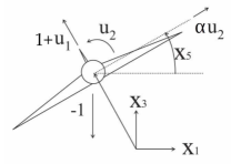
Let $a_{1},a_{2}$ be positive constants and consider the compact convex control constraint set

(77) $$U\>=\>[-a_{1},a_{1}]\,\times\,[-a_{2},a_{2}].$$

Introduce also the quadratic running cost

(78) $$g(x,u)\>\,=\>\,\frac{\lambda_{1}}{2}\,\|x\|^{2}\>+\>\frac{\lambda_{2}}{2}\,\|u\|^{2}\quad\forall x\in\mathbb{R}^{6}\quad\forall u\in\mathbb{R}^{2}$$

with positive constants $\lambda_{1},\lambda_{2}$. It is not difficult to verify that a quadratic local CLF $V_{\mathrm{loc}}(\cdot)$ can be constructed via linearization as described in Remark A.2.2 of Subsection A.2.1 in Online_App the appendix and that Theorems 2.20, 2.24, 2.25, 2.27 and 2.28 can be used with the running cost (78) and with the mentioned local CLF.

We take

(79) $$\alpha\,=\,0.1,\quad a_{1}\,=\,a_{2}\,=\,5,\quad\lambda_{1}\,=\,0.2,\quad\lambda_{2}\,=\,0.04.$$

The algebraic Riccati equation (see (A.14) in Online_App the appendix) was numerically solved via the care routine in the GNU Octave environment (the care routine in the MATLAB environment can be used as well). The range of appropriate levels $c$ was approximated with the help of the related recommendations in Subsection A.2.1 of Online_App the appendix (in order to handle possible multi-extremality, $20$ initial guesses were randomly generated for each of the corresponding finite-dimensional optimization problems). We finally selected

(80) $$c\,=\,0.017.$$

However, when trying to compute the CLF for the considered six-dimensional (three-degree-of-freedom) system at some states even not far from $\Omega_{c}$ via a characteristics based implementation similar to that used in Example 5.1, we faced huge difficulties in achieving a suitable shooting accuracy in the auxiliary problem for the reverse-time characteristics (even with the implicit Rosenbrock scheme [71, §17.5.1] used instead of the explicit Runge–Kutta scheme for numerical integration of ODEs). We hence used the ACADO Toolkit [48, 49] implementing a direct approximation method for optimal open-loop control problems. The other software packages mentioned in Subsection A.2.3 of Online_App the appendix involve more advanced and efficient direct collocation techniques and could also be applied. The ACADO Toolkit was chosen due to its relative simplicity, and also because its capabilities were enough for the purposes of this example. Regarding the characteristics based framework of Subsection A.2.2 in Online_App the appendix, it may help to numerically treat the current example if its implementation is modified in order to involve also multiple shooting or indirect collocation as applied to the characteristic system (see the general discussion of these techniques, e. g., in [76, 77]), but we leave that for future investigation.

We launched the ACADO Toolkit with the multiple shooting option, the maximum time horizon $20$, the tolerance $10^{-6}$ for the default Runge–Kutta integrator, the Karush–Kuhn–Tucker tolerance $10^{-4}$ (involved in the practical convergence criterion for the sequential quadratic programming algorithm), and with $40$ control intervals (these were time subintervals of equal length, and the constrained numerical optimization was performed over piecewise constant control strategies which might switch only at the endpoints of the subintervals).

For testing the performance and robustness of the MPC algorithm formulated in the beginning of Subsection A.2.4 in Online_App the appendix, we also consider a stochastic perturbation of the system (76). The noise is included in the second, fourth, and sixth dynamical equations (describing the accelerations for the three degrees of freedom). Let us write the resulting system:

(81) $$\left\{\begin{aligned} &\dot{x}_{1}(t)\>\>=\>\>x_{2}(t),\\ &\mathrm{d}x_{2}(t)\>\>=\>\>(-(1+u_{1}(t))\,\sin\,x_{5}(t)\,\,+\,\,\alpha\,u_{2}(t)\,\cos\,x_{5}(t))\>\mathrm{d}t\>\,+\>\,\sigma_{2}\,\mathrm{d}w_{2}(t),\\ &\dot{x}_{3}(t)\>\>=\>\>x_{4}(t),\\ &\mathrm{d}x_{4}(t)\>\>=\>\>((1+u_{1}(t))\,\cos\,x_{5}(t)\,\,+\,\,\alpha\,u_{2}(t)\,\sin\,x_{5}(t)\,\,-\,\,1)\>\mathrm{d}t\>\,+\>\,\sigma_{4}\,\mathrm{d}w_{4}(t),\\ &\dot{x}_{5}(t)\>\>=\>\>x_{6}(t),\\ &\mathrm{d}x_{6}(t)\>\>=\>\>u_{2}(t)\,\mathrm{d}t\>\,+\>\,\sigma_{6}\,\mathrm{d}w_{6}(t),\\ &t\geqslant 0,\\ &x(0)\,=\,x^{0}\,\in\,\mathbb{R}^{6}.\end{aligned}\right.$$

Here $x^{0}$ is a deterministic initial state, $\sigma_{2}$, $\sigma_{4}$, and $\sigma_{6}$ are nonnegative constants (noise intensity parameters), $\,(w_{2}(\cdot),w_{4}(\cdot),w_{6}(\cdot))\,$ is a three-dimensional standard Brownian motion (Wiener process) on the time interval $[0,+\infty)$, and the stochastic ordinary differential equations are understood in the Itô sense. An open-loop control strategy can also represent a stochastic process if it is obtained from a closed-loop map. Let us assess the control performance (quality) on a finite time interval $[0,T]$ through the mean value

(82) $$\mathbb{E}\left[\int\limits_{0}^{T}\|x(t)\|\>\mathrm{d}t\right]\>\,=\>\,\int\limits_{0}^{T}\mathbb{E}\,\|x(t)\|\>\mathrm{d}t.$$

The lower this value, the higher the control quality. The control goal is therefore interpreted as mitigating the random vibrations whose strength on $[0,T]$ is given by (82).

We select

(83) $$x^{0}\>=\>\left(2,\,3,\,4,\,1,\,\frac{\pi}{3}\,,\,1\right)^{\top}$$

(as in [73, Section 5]),

(84) $$T\,=\,15,\quad\sigma_{2}\,=\,\sigma_{4}\,=\,\sigma_{6}\,=\,\sigma,$$

and consider the two cases

(85) $$\sigma\,=\,0\>\>\mbox{(the deterministic case)}\>\>\>\mbox{and}\>\>\>\sigma\,=\,0.08.$$

According to the MPC algorithm, we implemented the piecewise constant control policy that was recomputed every $\,\Delta t_{\mathrm{recomp.}}\,=\,0.1\,$ time units as the stabilizing control action at the current state. When the state lied outside $\Omega_{c}$, the control action was approximated by applying the ACADO Toolkit to the original deterministic system. Otherwise, the value of the locally stabilizing linear feedback (as mentioned in Subsection A.2.1 of Online_App the appendix) at the current state in $\Omega_{c}$ was used. The Itô stochastic differential equations were solved via the Euler–Maruyama scheme that coincides with the Milstein scheme if the noise intensity matrix is constant and diagonal [78, 79]. The latter condition obviously holds for the system (81). The corresponding time step was set as $\,\Delta t_{\mathrm{SDE}}=10^{-5}$. Under certain smoothness and Lipschitz continuity conditions on the drift vector function and noise intensity matrix function, the Milstein scheme has the first strong convergence order (while the order of the Euler–Maruyama scheme in general equals $0.5$ if the noise intensity matrix is not constant). The first order of accuracy should be preserved in our MPC implementation, because the control policy is piecewise constant and the ratio $\>\Delta t_{\mathrm{recomp.}}\,/\,\Delta t_{\mathrm{SDE}}\>=\>10^{4}\>$ is integer.

The black solid curves in Fig. 8 indicate estimates of the mean values $\,\mathbb{E}\,\|x(t)\|\,$ and standard deviations $\,\sqrt{\mathrm{Var}\,\|x(t)\|}\,$ on the time interval $[0,T]$ for our MPC implementation. The deterministic and stochastic cases (85) are illustrated. For the stochastic case, $N=200$ Monte Carlo iterations were performed, and $x^{[i]}(\cdot)$ denotes the state trajectory at the $i$-th iteration, $i=\overline{1,N}$.

Figure 8: Estimates of the mean values $\,\mathbb{E}\,\|x(t)\|\,$ and standard deviations $\,\sqrt{\mathrm{Var}\,\|x(t)\|}\,$ for the original and constrained versions of the stabilizing feedback control law of Fantoni et al. [73, 74] and for the MPC implementation in Example 5.2. For the noise intensity parameter $\,\sigma_{2}=\sigma_{4}=\sigma_{6}=\sigma,\,$ the two cases (85) are considered. In order to see the graphs clearer, we do not fix the same scale for the vertical axes in the subfigures.

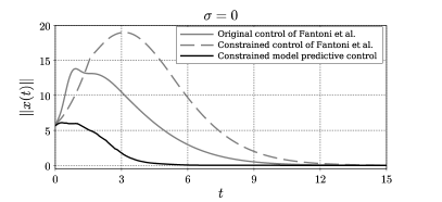
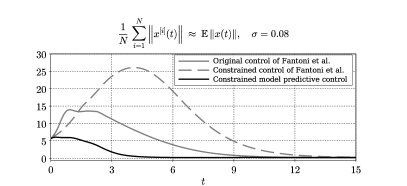
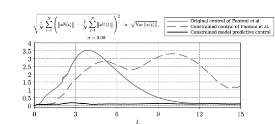
For comparison, we also integrated the systems (76) and (81) with the substituted continuous feedback control strategy that was developed and tested on real experiments by Fantoni et al. [73, 74]. The corresponding analytical representation was obtained after a change of the state and control variables that transformed the system (76) to a certain form without the coupling coefficient $\alpha$. This strategy was established to be locally stabilizing for the deterministic PVTOL system and to have a rather wide region of asymptotic null-controllability (see [73, Theorem 3.1] or [74, Theorem 1]). It has to be noted that the expressions for the first and second time derivatives of the auxiliary variable $r_{1}$ in [74, (16) and (17) on page 414] are incorrectly written ($2\,/\cos\,\theta\,$ in the formula for $\dot{r}_{1}$ should be replaced with $\,2\,\tan\,\theta,\,$ and the formula for $\ddot{r}_{1}$ should be accordingly modified). However, there is evidence that the correct relations were used in the further theoretical and practical investigation of [74]. In Fig. 8, the solid gray curves correspond to the original strategy of Fantoni et al., while the dashed gray curves indicate its constrained (saturating) version defined as the orthogonal projection to the compact convex control constraint set (77). The latter control law was not considered by Fantoni et al., and we tested it to see how the saturation would reduce the control performance. The Euler–Maruyama scheme was used with the same stepsize $\,\Delta t_{\mathrm{SDE}}=10^{-5},\,$ and the number of Monte Carlo iterations was again $N=200$. The explicit control representations could be handled very fast, so no MPC had to be arranged.

Fig. 8 shows that the constrained MPC has an essentially better performance than the original unconstrained strategy of Fantoni et al. and the saturating version of the latter. The higher robustness of the MPC with respect to stochastic uncertainties can be seen as well. In general, random vibrations can be effectively attenuated only for moderate noise intensities.

The average runtime of computing the CLF and the related control action at a single state outside $\Omega_{c}$ via the ACADO Toolkit was around 5 seconds on our relatively weak PC. This is much faster and more efficient compared to using our characteristics based implementation, although the latter is more justified from the theoretical point of view. Besides, more advanced and accurate optimal control solvers building on direct collocation methods (see Subsection A.2.3 in Online_App the appendix) often work noticeably faster than ACADO. However, the computational cost of such MPC implementations may still be rather high for real-time engineering applications. In general, there is a crucial trade-off between increasing the overall control quality and speeding up the online control evaluation.

In Subsection A.2.4 of Online_App the appendix, we discuss how sparse grids can be incorporated in the MPC algorithm with the aim to make it faster though less accurate. For investigating the applicability of the modified MPC algorithm, we estimated the accuracy of a typical high-dimensional sparse grid interpolation technique in the current example. We used the source code of the C++ library SPARSE_INTERP_ND [80] involving Clenshaw–Curtis nodes, hierarchical Smolyak’s constructions, and weighted sums of polynomial interpolants. First, we built the Clenshaw–Curtis sparse grid of level $7$ consisting of $44689$ distinct nodes on the six-dimensional cube $[-1,1]^{6}$. At each of the nodes and also at $1000$ points randomly generated from the uniform distribution on $[-1,1]^{6}$, the CLF $V(\cdot)$ as well as the related control action and costate were approximated by means of the GPOPS–II software [42, 43] (the latter involves direct collocation and is in general more effective than ACADO). In order to reduce the interpolation errors caused by the nonsmoothness of the CLF and the discontinuity of the costate on the surface $l_{c}=\partial\Omega_{c}$, we decreased the parameter $c$ to $4\cdot 10^{-4}$ and hence reduced the area of $l_{c}$ (however, it becomes more difficult to solve exit-time optimal control problems after reducing terminal sets). For the numerical optimization via GPOPS–II, the IPOPT nonlinear programming solver and the default collocation method were selected, and the corresponding tolerance was set as $10^{-7}$. Regarding the mesh refinement algorithm, we used the Patterson–Rao and Liu–Rao–Legendre methods with default parameters (if the numerical optimization process for a particular initial state did not converge with the Patterson–Rao mesh refinement option, it was rerun with the Liu–Rao–Legendre option). With the help of the obtained data, we then evaluated the errors of the sparse grid interpolation at the $1000$ randomly generated states (the values computed directly via GPOPS–II were compared with the interpolation estimates). The average relative errors turned out to be very large, more than $50\%$ for the CLF as well as for the related feedback control and costate. The infinitesimal decrease condition for the CLF $V(\cdot)$ was violated at more than half of the selected states after substituting the costate interpolation estimates instead of the gradient of $V(\cdot)$. One might think of considering a higher-level sparse grid, but the number of nodes and the complexity of interpolation would then dramatically increase, while the accuracy still might not become acceptable. Note also that the cube $[-1,1]^{6}$ may not be large enough for practical purposes, while the interpolation for the sparse grid of the same type and level on a larger parallelepiped is even less accurate.

The sparse grid interpolation was therefore highly inaccurate in this example, even though similar tests for other optimal control problems in [35] were successful. Thus, the range of applicability of sparse grid frameworks to solving feedback control problems and to reducing the complexity of online computations for MPC is a relevant subject of future research. Other techniques of scattered data interpolation, such as the Kriging method originally arising from geostatistics (see, e. g., [71, §3.7]), may be tested as well. ∎

6 Conclusion

In this work, we used exit-time optimal control settings in order to obtain global CLF characterizations, which could lead to curse-of-dimensionality-free approaches to feedback stabilization for certain classes of deterministic nonlinear control systems described by ODEs. Both theoretical and practical aspects were investigated. The computation of the values of the CLFs and stabilizing feedbacks at any selected states could be reduced to finite-dimensional nonlinear programming problems via characteristics based or direct approximation techniques as applied to specific exit-time optimal control problems. Recall that the direct numerical frameworks are less justified from a theoretical perspective but may be more robust in computations, compared to using the method of characteristics. We also indicated that our framework could be incorporated in MPC schemes for online stabilization.

Unlike Example 5.1 with two-dimensional state space, Example 5.2 with six-dimensional state space could not be successfully treated via our characteristics based numerical implementation. We hence employed a direct approximation technique for Example 5.2. The range of practical applicability of characteristics based frameworks to exit-time optimal control problems arising in stabilization problems with relatively high state space dimensions is worth studying further. In particular, an efficient implementation may combine the framework of Subsection A.2.2 in Online_App the appendix with multiple shooting or indirect collocation [76, 77].

Another remaining dilemma is how to reasonably reduce the complexity of online computations in the related MPC schemes, while preserving a suitable level of accuracy and the stabilization property. In Example 5.2, a typical sparse grid framework could not achieve that, although similar tests for other optimal control problems in [35] showed acceptable results. Thus, the range of applicability of sparse grids to solving feedback control problems may also be an interesting subject of future research. Other techniques of scattered data interpolation (such as the Kriging method [71, §3.7]) may be additionally tested. Moreover, since the characteristics based techniques and advanced direct collocation methods enable costate estimation for optimal control problems (recall the relation between the costates and the gradient of a value function, as well as the local Lipschitz continuity properties in Theorems 2.20, 3.9), it is relevant to design methods for constructing piecewise affine global CLFs in relatively high dimensions. The framework of [81] may help in that effort.

Online_App

Appendix A.1 Proofs of some auxiliary results

A.1.1 Proof of Lemma 2.12

Lemma 2.12.

If $E\subseteq\mathbb{R}^{n}$ is an open set and a function $\>\varphi\,\colon\,E\to\mathbb{R}\>$ is Lipschitz continuous with constant $C>0$, then

(A.1) $$\|\zeta\|\,\leqslant\,C\sqrt{n}\quad\forall\,\zeta\,\in\,\mathrm{D}^{-}_{\mathrm{P}}\varphi(x)\quad\forall x\in E.$$

Proof.

Let $x\in E$ and $\,\zeta\in\mathrm{D}^{-}_{\mathrm{P}}\varphi(x)$. According to the Lipschitz continuity of $\varphi(\cdot)$ and the definition of a proximal subgradient (see [59, p. 5]), there exist positive numbers $\varepsilon_{0},\sigma$ (depending on $x$) such that $\,\mathrm{B}_{\varepsilon_{0}}(x)\subseteq E\,$ and

(A.2) $$C\,\|x^{\prime}-x\|\>\>\geqslant\>\>\varphi(x^{\prime})\>-\>\varphi(x)\>\>\geqslant\>\>\left<\zeta,\,x^{\prime}-x\right>\>-\>\sigma\,\|x^{\prime}-x\|^{2}$$

for all $\,x^{\prime}\in\mathrm{B}_{\varepsilon_{0}}(x)$. For every $\>i\,\in\,\{1,2,\ldots,n\},\>$ let $e_{i}\in\mathbb{R}^{n}$ be such that its $i$-th coordinate equals $1$ and all the other coordinates vanish. Take arbitrary $\>i\,\in\,\{1,2,\ldots,n\}\>$ and $\varepsilon\in(0,\varepsilon_{0})$. Then (A.2) reduces to $\>C\>\geqslant\>\left<\zeta,e_{i}\right>\,-\,\sigma\varepsilon\>$ for $\>x^{\prime}\,=\,x+\varepsilon e_{i}\>$ and to $\>C\>\geqslant\>-\left<\zeta,e_{i}\right>\,-\,\sigma\varepsilon\>$ for $\>x^{\prime}\,=\,x-\varepsilon e_{i}$. As $\varepsilon\to+0$, one obtains $\,\left|\left<\zeta,e_{i}\right>\right|\leqslant C$. This leads directly to (A.1). ∎

A.1.2 Proof of Proposition 2.29

First, recall the notation

(A.3) $$H(x,u,p,\tilde{p})\>\,\stackrel{{\scriptstyle\mathrm{def}}}{{=}}\>\,\left<p,f(x,u)\right>\>+\>\tilde{p}\,g(x,u),$$

$$\mathcal{H}(x,p,\tilde{p})\>\,\stackrel{{\scriptstyle\mathrm{def}}}{{=}}\>\,\min_{u^{\prime}\,\in\,U}\,H(x,u^{\prime},p,\tilde{p}),$$

$$U^{*}(x,p,\tilde{p})\>\,\stackrel{{\scriptstyle\mathrm{def}}}{{=}}\>\,\mathrm{Arg}\min_{u^{\prime}\,\in\,U}\,H(x,u^{\prime},p,\tilde{p})$$

$$\forall\>(x,u,p,\tilde{p})\>\in\>G\times U\times\mathbb{R}^{n}\times\mathbb{R}$$

(see (32), (37)), as well as the characteristic Cauchy problems

(A.4) $$\left\{\begin{aligned} &\dot{x^{*}}(t)\>\>=\>\>\mathrm{D}_{p}H(x^{*}(t),\,u^{*}(t),\,p^{*}(t),\,\tilde{p}^{*})\>\>=\>\>f(x^{*}(t),\,u^{*}(t)),\\ &\dot{p^{*}}(t)\>\>=\>\>-\mathrm{D}_{x}H(x^{*}(t),\,u^{*}(t),\,p^{*}(t),\,\tilde{p}^{*})\\ &\qquad\>\>=\>\>-(\mathrm{D}_{x}f(x^{*}(t),\,u^{*}(t)))^{\top}\>p^{*}(t)\>\,-\>\,\tilde{p}^{*}\>\mathrm{D}_{x}g(x^{*}(t),\,u^{*}(t)),\\ &u^{*}(t)\>\in\>U^{*}(x^{*}(t),\,p^{*}(t),\,\tilde{p}^{*}),\\ &t\>\,\in\>\,I(x_{0},\,u^{*}(\cdot))\>\,\stackrel{{\scriptstyle\mathrm{def}}}{{=}}\>\,\begin{cases}[0,\,T_{\Omega_{c}}(x_{0},\,u^{*}(\cdot))],&T_{\Omega_{c}}(x_{0},\,u^{*}(\cdot))\><\>+\infty,\\ [0,+\infty),&T_{\Omega_{c}}(x_{0},\,u^{*}(\cdot))\>=\>+\infty,\end{cases}\\ &x^{*}(0)\,=\,x_{0},\quad p^{*}(0)\,=\,p_{0}\end{aligned}\right.$$

(see (39)), where $\>(x_{0},p_{0},\tilde{p}^{*})\>\in\>G\,\times\,\mathbb{R}^{n}\,\times\,[0,+\infty)$.

Proposition 2.29.

Under the conditions of Theorem 2.28, the Hamiltonian is conserved along any solution of the characteristic Cauchy problem (A.4) with $\>(x_{0},p_{0},\tilde{p}^{*})\>\in\>G\,\times\,\mathbb{R}^{n}\,\times\,[0,+\infty)$.

Proof.

By using the representation of directional derivatives of minimum functions (see, e. g., [82, Theorem I.3.4], which considers maximum functions, but can be similarly reformulated for minimum functions), one can verify that

(A.5) $$\frac{\mathrm{d}}{\mathrm{d}t}\>\mathcal{H}(x^{*}(t),\,p^{*}(t),\,\tilde{p}^{*})\>\,=\>\,0\quad\mbox{for almost all}\>\>\,t\,\in\,I(x_{0},\,u^{*}(\cdot)).$$

Since $x^{*}(\cdot)$ and $p^{*}(\cdot)$ are absolutely continuous on every compact subset of $\,I(x_{0},\,u^{*}(\cdot))\,$ and $\mathcal{H}(\cdot,\cdot,\cdot)$ is Lipshitz continuous on every compact subset of $\,G\times\mathbb{R}^{n}\times\mathbb{R}\,$ (due to, e. g., [82, Remark I.3.2]), the function $\>I(x_{0},\,u^{*}(\cdot))\,\ni\,t\>\longmapsto\>\mathcal{H}(x^{*}(t),\,p^{*}(t),\,\tilde{p}^{*})\>$ is also absolutely continuous on any compact subset of $\,I(x_{0},\,u^{*}(\cdot))$. Hence, (A.5) implies that the latter function is constant on $\,I(x_{0},\,u^{*}(\cdot))$. ∎

Appendix A.2 Further details on implementing the curse-of-dimensionality-free approach to CLF approximation and feedback stabilization

This section accompanies Section 4 and discusses how to practically evaluate the global CLF $V(\cdot)$ (or, equivalently, the Kruzhkov transformed CLF $v(\cdot)$) together with the corresponding feedback strategy at any selected state in $G$, based on the theoretical results of Section 2 (similar considerations excluding local CLF construction can be applied to the setting of Section 3). It is also pointed out that our framework can be incorporated in model predictive control schemes for online stabilization. For convenience, the description is divided into a number of subsections.

A.2.1 Construction of a local CLF

The results of Section 2 were established under the a priori assumption that a local CLF with desired properties could be obtained. Analytical construction of local CLFs may in general be a difficult task, if one first considers the ideal case of unconstrained control inputs and tries to exactly find the corresponding global CLF (by using, e. g., the results of [1, §9.4] or [2, Chapter 5]), which can then work locally in case of pointwise control constraints. Besides, for a number of well-known continuous-time mechanical models, the local or global asymptotic stabilization properties of certain feedbacks are derived by means of nonstrict Lyapunov functions, such that the right-hand sides in the related infinitesimal decrease conditions vanish not only at the origin [7, 8, 9, 83, 84, 85]. However, Definition 2.5 of CLFs and the sufficient conditions of local asymptotic null-controllability used in Remark 2.9 include the strictness.

In this subsection, we propose a linearization based numerical technique for building quadratic local CLFs under some additional conditions, with the considerations of [53, Section 3] serving as an important motivation. Those considerations can also be employed for constructing quadratic local CLFs under the same assumptions. Although the technique presented in the current subsection is less elegant and may be more computationally expensive, it is more straightforward to use and does not restrict the right-hand sides in the decrease conditions for the resulting local CLFs necessarily to quadratic functions (in contrast to the approach of [53, Section 3]).

Assumption A.2.1.

In addition to Assumption 2.1, suppose that $\,0_{m}\in\mathrm{int}\,U$, $\,f(0_{n},0_{m})=0_{n},\,$ the function $f(\cdot,\cdot)$ is continuously differentiable, and the linearization

(A.6) $$\left\{\begin{aligned} &\dot{x}(t)\>=\>A\,x(t)\,+\,B\,u(t),\quad t\geqslant 0,\\ &x(0)\,=\,x_{0}\,\in\,G,\\ &u(\cdot)\>\in\>\mathcal{U}\>\stackrel{{\scriptstyle\mathrm{def}}}{{=}}\>L^{\infty}_{\mathrm{loc}}([0,+\infty),\,U),\\ &A\>\stackrel{{\scriptstyle\mathrm{def}}}{{=}}\>\mathrm{D}_{x}f(0_{n},0_{m})\>\in\>\mathbb{R}^{n\times n},\quad B\>\stackrel{{\scriptstyle\mathrm{def}}}{{=}}\>\mathrm{D}_{u}f(0_{n},0_{m})\>\in\>\mathbb{R}^{n\times m},\end{aligned}\right.$$

of the system (1) is asymptotically null-controllable.

Due to [67, §5.8, Theorem 19], Assumption A.2.1 ensures the existence of a positive definite matrix $P\in\mathbb{R}^{n\times n}$ and a matrix $S\in\mathbb{R}^{m\times n}$ such that the functions

(A.7) $$\breve{V}(x_{0})\>=\>\left<Px_{0},\,x_{0}\right>,\>\>\>\breve{u}(x_{0})\>=\>Sx_{0}\quad\forall x_{0}\in\mathbb{R}^{n}$$

are respectively a local quadratic CLF and a locally stabilizing linear feedback for (1) in some neighborhood of the origin $0_{n}$. One can search for such a neighborhood in the form of a sublevel set of $\breve{V}(\cdot)$.

In line with [67, §5.8, Proof of Theorem 19], the control matrix $S$ is selected so that $\>A+BS\,\in\,\mathbb{R}^{n\times n}\>$ becomes Hurwitz, and $P$ is a unique positive definite solution of the matrix equation

(A.8) $$(A+BS)^{\top}\,P\>+\>P\,(A+BS)\>\,=\>\,-\alpha I_{n\times n}$$

with a constant $\alpha>0$ (one has $\alpha=1$ in that proof, though any $\alpha>0$ would in fact work).

The gradient of $\breve{V}(\cdot)$ is given by

$$\mathrm{D}\breve{V}(x_{0})\>=\>2\,Px_{0}\quad\forall x_{0}\in\mathbb{R}^{n},$$

and the sublevel sets

(A.9) $$\breve{\Omega}_{r}\>\,\stackrel{{\scriptstyle\mathrm{def}}}{{=}}\>\,\{x\in\mathbb{R}^{n}\>\colon\>\breve{V}(x)\,\leqslant\,r\}\quad\forall r>0$$

are closed ellipsoidal domains in $\mathbb{R}^{n}$. If a level $c^{\prime}>0$ satisfies

(A.10) $$\begin{array}[]{c}\breve{\Omega}_{c^{\prime}}\,\subset\,G,\\ \left<\mathrm{D}\breve{V}(x),\>f(x,\breve{u}(x))\right>\>\,<\>\,0\quad\forall\,x\,\in\,\breve{\Omega}_{c^{\prime}}\setminus\{0_{n}\},\\ \breve{u}(x)\in U\quad\forall x\in\breve{\Omega}_{c^{\prime}},\end{array}$$

then one can take

(A.11) $$\Omega\>=\>\mathrm{int}\,\breve{\Omega}_{c^{\prime}},\quad c\in(0,c^{\prime}),\quad\Omega_{c}=\breve{\Omega}_{c}$$

and select a local CLF and a locally stabilizing feedback as

(A.12) $$V_{\mathrm{loc}}(x)\,\stackrel{{\scriptstyle\mathrm{def}}}{{=}}\,\breve{V}(x),\>\>\>u_{\mathrm{loc}}(x)\,\stackrel{{\scriptstyle\mathrm{def}}}{{=}}\,\breve{u}(x)\quad\forall x\in\Omega.$$

The greater such a level $c$, the wider the target set $\Omega_{c}$, and, hence, the easier to numerically solve the exit-time optimal control problem (21). This leads to the problem of finding the supremum $c_{\sup}$ of all suitable levels, which can be practically treated by testing the nodes of a grid on the interval $[0,\tilde{c}]$ with a sufficiently large right endpoint $\tilde{c}>0$. For each node, an appropriate finite-dimensional optimization problem should be numerically solved. Finally, it is reasonable to select $c$ somewhat lower than $c_{\sup}$, so that $\>\left<\mathrm{D}V_{\mathrm{loc}}(x),\>f(x,u_{\mathrm{loc}}(x))\right>\>$ is not very close to zero at states $x$ near the boundary $\,l_{c}=\partial\Omega_{c}$.

Remark A.2.2.

If the asymptotic null-controllability condition in Assumption A.2.1 is replaced with the stronger exact null-controllability condition

(A.13) $$\mathrm{rank}\>\left[B,\,AB,\,A^{2}B,\,\ldots,\,A^{n-1}B\right]\>\,=\>\,n,$$

then the matrix $P\in\mathbb{R}^{n\times n}$ in (A.7) can be chosen as a unique positive definite solution of the algebraic Riccati equation

(A.14) $$A^{\top}P\>+\>PA\>-\>PBR^{-1}B^{\top}P\>+\>Q\>\,=\>\,0_{n\times n}$$

with arbitrary positive definite matrices $\,Q\in\mathbb{R}^{n\times n}$, $R\in\mathbb{R}^{m\times m},\,$ and the control matrix in (A.7) can be taken as $\,S=-R^{-1}B^{\top}P\,$ (see, e. g., [6, Chapter VII, §3.3]). In this case, (A.7) gives the value function and optimal feedback strategy for the infinite-horizon linear-quadratic optimal control problem

(A.15) $$\left\{\begin{aligned} &\dot{x}(t)\>\,=\>\,A\,x(t)\>+\>B\,u(t),\quad t\geqslant 0,\\ &x(0)\,=\,x_{0}\,\in\,\mathbb{R}^{n},\\ &u(\cdot)\>\in\>L_{\mathrm{loc}}^{\infty}([0,+\infty),\,\mathbb{R}^{m}),\\ &\int\limits_{0}^{+\infty}(\left<Q\,x(t),\,x(t)\right>\>+\>\left<R\,u(t),\,u(t)\right>)\>\mathrm{d}t\>\,\longrightarrow\>\,\min,\end{aligned}\right.$$

with unconstrained control inputs. ∎

A.2.2 Using the characteristics based representation of the value function

This subsection describes the use of the characteristics based representation of $v(\cdot)$ in $\mathcal{D}_{0}\setminus\Omega_{c}$ given by Theorem 2.28, whose formulation is repeated here for convenience.

Theorem 2.28.

Let Assumptions 2.1, 2.7, 2.15, 2.21 and 2.23 hold. For any initial state $\,x_{0}\,\in\,\mathcal{D}_{0}\setminus\Omega_{c},\,$ the Kruzhkov transformed value $v(x_{0})$ defined by (20), (21), (36) is the minimum of

(A.16) $$1\>\>-\>\>\exp\left\{-\int\limits_{0}^{T_{\Omega_{c}}(x_{0},\,u^{*}(\cdot))}g(x^{*}(t),\,u^{*}(t))\>\mathrm{d}t\>\,-\>\,c\right\}$$

over the solutions of the characteristic Cauchy problems (A.4) for all extended initial adjoint vectors

(A.17) $$(p_{0},\tilde{p}^{*})\>\,\in\>\,\{(p,\tilde{p})\>\colon\>p\in\mathbb{R}^{n},\>\>\tilde{p}\in\{0,1\}\}.$$

Moreover, the same value is obtained when minimizing over the bounded set

(A.18) $$(p_{0},\tilde{p}^{*})\>\,\in\>\,\{(p,\tilde{p})\>\in\>\mathbb{R}^{n}\times\mathbb{R}\>\colon\>\|(p,\tilde{p})\|\>=\>1,\>\>\,\tilde{p}\geqslant 0\},$$

or even over its subset

(A.19) $$(p_{0},\tilde{p}^{*})\>\,\in\>\,\{(p,\tilde{p})\>\in\>\mathbb{R}^{n}\times\mathbb{R}\>\colon\>\|(p,\tilde{p})\|\>=\>1,\>\>\,\tilde{p}\geqslant 0,\>\>\,\mathcal{H}(x_{0},p,\tilde{p})\>=\>0\}.$$

In order to ensure the uniqueness of the solutions of the characteristic Cauchy problems (A.4) in the normal case $\tilde{p}^{*}>0$, the following conditions are imposed.

Assumption A.2.3.

The extremal control map $U^{*}(x,p,\tilde{p})$ (see (A.3)) is singleton for $\tilde{p}>0$, and the corresponding function defined on $\>G\,\times\,\mathbb{R}^{n}\,\times\,(0,+\infty)\>$ and taking values in $U$ is locally Lipschitz continuous.

This often holds if, for instance, the running cost is regularized by adding a suitable control-dependent term. In the abnormal case $\tilde{p}^{*}=0$, there typically exist states and adjoint vectors for which the extremal control map is nonsingleton, regardless of the running cost. However, one can expect that abnormal characteristics would rarely be optimal, since they do not take the running cost into account. If the extremal control map on a characteristic trajectory becomes nonsingleton at some time during computations, one can select any extremal control action at this time. Note also that, for some particular classes of optimal control problems, an additional analysis via Pontryagin’s principle may allow characteristics based methods to be modified so that singular regimes are explicitly handled and the nonuniqueness in the choice of extremal control actions is avoided (see [33, Examples 3.14 and 3.15] related to the case of a fixed finite horizon).

A.2.2.1 Practical specification of exit times and the domain of asymptotic null-controllability

Next, recall the representation of the domain of asymptotic null-controllability $\mathcal{D}_{0}$ in Theorem 2.27:

(A.20) $$\mathcal{D}_{0}\>\>=\>\>\{x_{0}\in G\>\colon\>V(x_{0})\,<\,+\infty\}\>\>=\>\>\{x_{0}\in G\>\colon\>v(x_{0})\,<\,1\}.$$

Before evaluating the CLF at a particular state $x_{0}\in G$, one usually does not know if $x_{0}\in\mathcal{D}_{0}$ or not. Even if the initial state lies in $\mathcal{D}_{0}$, there may still exist extended initial adjoint vectors $(p_{0},\tilde{p}^{*})$ that generate characteristic trajectories with infinite exit time and with the cost (A.16) equal to $1$.

Let us provide a practical rule to determine costs and exit (terminal) times during numerical integration of the characteristic Cauchy problems (A.4). A priori, it is reasonable to fix a sufficiently large finite upper bound $T_{\max}>0$ for exit times, even though this is in general a heuristic choice. Take also a sufficiently small parameter $\varepsilon\in(0,1)$. It is proposed to stop integrating the characteristic system when at least one of the following conditions starts to hold:

• the a priori selected upper bound for terminal times is reached, i. e., $t=T_{\max}$;

• the target set is entered, i. e., $x^{*}(t)\in\Omega_{c}$;

• the accumulated cost becomes very close to the maximum value $1$, i. e.,

  $$1\>\>-\>\>\exp\left\{-\int\limits_{0}^{t}g(x^{*}(s),\,u^{*}(s))\>ds\>\,-\>\,c\right\}\>\>\geqslant\>\>1-\varepsilon.$$

These three cases accordingly define practical exit times. In Case 2, the cost is specified as (A.16), while, in Cases 1 and 3, it is set as $1-\varepsilon$.

Let $\>\hat{v}\colon\>G\setminus\Omega_{c}\,\to\,[0,\,1-\varepsilon]\>$ be the approximation of $v(\cdot)$ in $G\setminus\Omega_{c}$ obtained by incorporating the aforementioned arguments in a numerical method building on Theorem 2.28. Select one more parameter $\varepsilon_{1}\in(0,1)$, which is sufficiently small but not less than $\varepsilon$. Then the domain $\mathcal{D}_{0}$ can be approximated by its inner estimate

(A.21) $$\hat{\mathcal{D}}_{0}\>\>\stackrel{{\scriptstyle\mathrm{def}}}{{=}}\>\>\Omega_{c}\>\,\cup\>\,\{x_{0}\,\in\,G\setminus\Omega_{c}\>\colon\>\hat{v}(x_{0})\,<\,1-\varepsilon_{1}\}.$$

A.2.2.2 An auxiliary problem for finding an appropriate initial guess for the main optimization problem

Let us refer to the finite-dimensional optimization problem formulated in Theorem 2.28 as the main problem. The cost function in this problem may be essentially multi-extremal for some initial states $x_{0}\in G$. There may in particular exist a relatively large subset of (A.18) consisting of the extended initial adjoint vectors $(p_{0},\tilde{p}^{*})$ for which the state trajectories of (A.4) do not reach the target set $\Omega_{c}$ and the approximate cost defined above equals $1-\varepsilon$. It is hence reasonable first to introduce an auxiliary problem, whose solution can then serve as an initial guess for an iterative algorithm applied to the main problem.

Consider the characteristic system rewritten in reverse time $\tau$, that is,

(A.22) $$\left\{\begin{aligned} &\frac{\mathrm{d}\hat{x}^{*}(\tau)}{\mathrm{d}\tau}\>\>=\>\>-\mathrm{D}_{p}H(\hat{x}^{*}(\tau),\,\hat{u}^{*}(\tau),\,\hat{p}^{*}(\tau),\,\tilde{p}^{*})\>\>=\>\>-f(\hat{x}^{*}(\tau),\,\hat{u}^{*}(\tau)),\\ &\frac{\mathrm{d}\hat{p}^{*}(\tau)}{\mathrm{d}\tau}\>\>=\>\>\mathrm{D}_{x}H(\hat{x}^{*}(\tau),\,\hat{u}^{*}(\tau),\,\hat{p}^{*}(\tau),\,\tilde{p}^{*})\\ &\qquad\quad\>\,=\>\>(\mathrm{D}_{x}f(\hat{x}^{*}(\tau),\,\hat{u}^{*}(\tau)))^{\top}\>\hat{p}^{*}(\tau)\>\,+\>\,\tilde{p}^{*}\>\mathrm{D}_{x}g(\hat{x}^{*}(\tau),\,\hat{u}^{*}(\tau)),\\ &\hat{u}^{*}(\tau)\>\in\>U^{*}(\hat{x}^{*}(\tau),\,\hat{p}^{*}(\tau),\,\tilde{p}^{*}),\\ &\tau\>\in\>I(\hat{x}^{*}(0),\,\hat{p}^{*}(0),\,\tilde{p}^{*}),\end{aligned}\right.$$

where $\>I(\hat{x}^{*}(0),\,\hat{p}^{*}(0),\,\tilde{p}^{*})\>$ is the maximum extendability time interval with zero left endpoint during which the related solutions emanating from $\>(\hat{x}^{*}(0),\,\hat{p}^{*}(0))\>$ satisfy $\>\hat{x}^{*}(\tau)\,\in\,G,\>$ and take also

(A.23) $$\hat{x}^{*}(0)\,\in\,\Omega_{c_{1}},\quad\hat{p}^{*}(0)\>\in\>\mathrm{N}(\hat{x}^{*}(0);\,\Omega_{c_{1}})$$

for some parameter $c_{1}\in(0,c]$. The conditions (A.23) come from Pontryagin’s principle for the exit-time optimal control problem with the target set

(A.24) $$\Omega_{c_{1}}\>\,\stackrel{{\scriptstyle\mathrm{def}}}{{=}}\>\,\left\{x\in\bar{\Omega}\,\colon\,V_{\mathrm{loc}}(x)\leqslant c_{1}\right\}\>\,\subseteq\>\,\Omega_{c}$$

instead of $\Omega_{c}$. The aim is to get to a selected state $x_{0}\in G$ as close as possible, which leads to a shooting problem. The level $c_{1}$ is allowed to be less than $c$ in order to make the shooting more robust, i. e., to increase the possibility that the resulting initial guess for the main optimization problem with $x_{0}\in\mathcal{D}_{0}$ generates a forward-time characteristic state trajectory reaching the original target set $\Omega_{c}$ within the fixed time interval $[0,T_{\max}]$. Note also that a similar reduction of a terminal sublevel set is used in [52] for increasing the robustness of a receding horizon stabilization algorithm.

Additional properties need to be imposed.

Assumption A.2.4.

$c_{1}\in(0,c]$ is a constant. Item 4 of Assumption 2.7 holds when $c$ is replaced with $c_{1}$ and $C_{3}$ remains the same. Item 4 of Assumption 2.15 holds when $c$ is replaced with $c_{1}$ and $C_{6}$ is replaced with $C^{\prime}_{6}\in(0,C_{6}]$.

Denote also

(A.25) $$l_{c_{1}}\>\,\stackrel{{\scriptstyle\mathrm{def}}}{{=}}\>\,\left\{x\in\bar{\Omega}\,\colon\,V_{\mathrm{loc}}(x)=c_{1}\right\}\>\,=\>\,\partial\Omega_{c_{1}}.$$

Assumption A.2.5.

The local CLF $V_{\mathrm{loc}}(\cdot)$ is continuously differentiable in $\Omega$, and, for any direction $\xi\in\mathbb{R}^{n}$ with $\|\xi\|=1$, there exists a unique state

(A.26) $$x^{*}_{\mathrm{term}}(\xi)\>\>\in\>\>l_{c_{1}}\>\,\cap\>\,\{\lambda\xi\>\colon\>\lambda>0\}.$$

Remark A.2.6.

Let Assumptions 2.1, 2.7 and A.2.4 hold. It is not difficult to verify that Assumption A.2.5 also holds if, for example, the following conditions are fulfilled:

• $\Omega$ is convex;

• $V_{\mathrm{loc}}(\cdot)$ is continuously differentiable and convex in $\Omega$ (the convexity of $V_{\mathrm{loc}}(\cdot)$ implies the convexity of its sublevel sets, such as $\Omega_{c}$ and $\Omega_{c_{1}}$);

• $V_{\mathrm{loc}}(\cdot)$ satisfies

  $$\left<x,\,\mathrm{D}V_{\mathrm{loc}}(x)\right>\>>\>0\quad\forall x\in l_{c_{1}}$$

  (this holds in particular for quadratic local CLFs).

∎

In line with Assumptions A.2.4, A.2.5 and the Hamiltonian vanishing condition in Pontryagin’s principle, the initial data (A.23) for the reverse-time characteristic system (A.22) is taken as

(A.27) $$\begin{array}[]{c}\hat{x}^{*}(0)\>=\>x^{*}_{\mathrm{term}}(\xi)\>\in\>l_{c_{1}},\quad\xi\in\mathbb{R}^{n},\quad\|\xi\|=1,\\ \hat{p}^{*}(0)\,\,=\,\,\varkappa\>\mathrm{D}V_{\mathrm{loc}}(\hat{x}^{*}(0)),\quad\varkappa\geqslant 0,\\ \mathcal{H}(\hat{x}^{*}(0),\>\hat{p}^{*}(0),\>\tilde{p}^{*})\,\,=\,\,0,\quad\tilde{p}^{*}\geqslant 0.\end{array}$$

By adopting the normalization condition $\>\|(\hat{p}^{*}(0),\,\tilde{p}^{*})\|\>=\>1,\>$ one obtains

(A.28) $$\tilde{p}^{*}\in[0,1],\quad\varkappa\>=\>\frac{\sqrt{1-(\tilde{p}^{*})^{2}}}{\|\mathrm{D}V_{\mathrm{loc}}(\hat{x}^{*}(0))\|}\,,$$

and $\>\mathrm{D}V_{\mathrm{loc}}(\hat{x}^{*}(0))\,\neq\,0_{n}\>$ due to the infinitesimal decrease condition on the local CLF and $\>\inf\>\{g(x,u)\>\colon\>x\in l_{c_{1}},\>\,u\in U\}\,\,>\,\,0\>$ (recall Assumptions 2.7, 2.15 and A.2.4). The latter properties also yield that, for any $\xi\in\mathbb{R}^{n}$ with $\|\xi\|=1$, the function

(A.29) $$[0,1]\>\ni\>\tilde{p}\>\>\longmapsto\>\>\mathcal{H}\left(x^{*}_{\mathrm{term}}(\xi),\>\>\frac{\sqrt{1-\tilde{p}^{2}}}{\|\mathrm{D}V_{\mathrm{loc}}(x^{*}_{\mathrm{term}}(\xi))\|}\,\,\mathrm{D}V_{\mathrm{loc}}(x^{*}_{\mathrm{term}}(\xi)),\>\>\tilde{p}\right)$$

is negative at $\tilde{p}=0$ and positive at $\tilde{p}=1$, i. e., at least one root $\tilde{p}^{*}$ exists and satisfies

(A.30) $$0<\tilde{p}^{*}<1$$

(which in particular excludes the abnormal case $\tilde{p}^{*}=0$). Possible multiple roots on $(0,1)$ can be numerically bracketed, for example, by using the zbrak routine from [71, §9.1]. Each of them is further handled, and a root with the best shooting performance is finally selected.

The shooting goal is to minimize the lowest deviation

(A.31) $$\min_{\tau\>\>\in\>\>[0,\,T_{\max}]\>\,\cap\>\,I(\hat{x}^{*}(0),\,\,\hat{p}^{*}(0),\,\,\tilde{p}^{*})}\>\left\|\hat{x}^{*}(\tau)\,-\,x_{0}\right\|^{2}$$

from a state $x_{0}\in G$ over the solutions of the reverse-time characteristic Cauchy problems (A.22), (A.27), (A.28). One therefore arrives at optimizing over the vectors $\xi$ on the unit sphere in $\mathbb{R}^{n}$, which can be parametrized as follows:

(A.32) $$\left\{\begin{aligned} &\xi_{1}\>=\>\prod_{i=1}^{n-1}\sin\,\theta_{i},\\ &\xi_{j}\>=\>\cos\,\theta_{j-1}\,\prod_{i=j}^{n-1}\sin\,\theta_{i},\quad j\,=\,\overline{2,\,n-1},\\ &\xi_{n}\>=\>\cos\,\theta_{n-1},\\ &0\leqslant\theta_{1}<2\pi,\quad 0\leqslant\theta_{j}\leqslant\pi,\quad j\,=\,\overline{2,\,n-1}.\end{aligned}\right.$$

The periodicity in the angles $\,\theta_{i}$, $i=\overline{1,n},\,$ allows for performing unconstrained optimization over them. Possible multi-extremality in the auxiliary problem can be treated by applying an iterative optimization method to a fixed number of random initial guesses generated according to the uniform angles distribution.

If $\>(\hat{x}^{*}(\cdot),\,\hat{p}^{*}(\cdot),\,\tilde{p}^{*})\>$ is an optimal shooting characteristic and $\tau^{\prime}$ is a minimizer in (A.31), then the extended adjoint vector

(A.33) $$\left(\frac{\hat{p}^{*}(\tau^{\prime})}{\tilde{p}^{*}}\,,\>1\right)$$

(normalized so as to make the last coordinate equal to $1$) can specify the initial guess for an iterative optimization method applied to the main problem for forward-time characteristics. The normalization in (A.33) allows for optimizing with respect to $p_{0}\in\mathbb{R}^{n}$ in the main problem, as well as for representing the gradient $\mathrm{D}V(\cdot)$ of the original value function along optimal characteristics in case $x_{0}\in\mathcal{D}_{0}$ ($V(x_{0})<+\infty$) directly via the adjoint variable (costate).

If $p_{0}$ is an optimal initial costate in the main problem (with $\tilde{p}^{*}=1$) for an initial state $x_{0}$, the optimal control action at this state is chosen from $\,U^{*}(x_{0},p_{0},1)$.

Even if $x_{0}\in\mathcal{D}_{0}$ and the optimal cost (A.31) in the auxiliary shooting problem is rather small, the related initial guess (A.33) for the main problem and also some neighboring adjoint vectors might still lead to a forward-time characteristic state trajectory that emanates from $x_{0}$ but does not reach the target set $\Omega_{c}$ within the time interval $[0,T_{\max}]$. In this situation, the shooting is not accurate enough, but the following technique for evaluating $v(x_{0})$ may be helpful. Select two sufficiently small positive parameters $\delta_{1},\delta_{2}$. If the square root of the optimal shooting cost (A.31) is less than $\delta_{1}$ and $\,\hat{x}_{0}=\hat{x}^{*}(\tau^{\prime})\,$ is the closest state to $x_{0}$ on the optimal shooting characteristic, then one can solve the main optimization problem (with $\tilde{p}^{*}=1$) for the initial state $\hat{x}_{0}$ and use the corresponding value $v(\hat{x}_{0})$ and optimal initial costate $\hat{p}_{0}$ in order to approximate $v(x_{0})$. More precisely, if $\>\|\hat{x}_{0}-x_{0}\|\,<\,\delta_{1}$ and $\>v(\hat{x}_{0})\,=\,1-e^{-V(\hat{x}_{0})}\,<\,1-\varepsilon,\>$ consider the first-order estimate

(A.34) $$\begin{array}[]{c}V_{1}(x_{0})\>\>\stackrel{{\scriptstyle\mathrm{def}}}{{=}}\>\>V(\hat{x}_{0})\>+\>\left<\hat{p}_{0},\,x_{0}-\hat{x}_{0}\right>,\quad V(\hat{x}_{0})\>=\>-\ln\,(1\,-\,v(\hat{x}_{0})),\\ v_{1}(x_{0})\>\stackrel{{\scriptstyle\mathrm{def}}}{{=}}\>1\,-\,e^{-V_{1}(x_{0})},\end{array}$$

and, if also $\>0\,\leqslant\,v_{1}(x_{0})\,<\,1-\varepsilon\>$ and $\>|v_{1}(x_{0})\,-\,v(\hat{x}_{0})|\><\>\delta_{2},\>$ take $\>v(x_{0})\,\approx\,v_{1}(x_{0})$. If at least one of the tested conditions does not hold, put $\>v(x_{0})\,\approx\,1-\varepsilon$. Moreover, the sought-after control action at the state $x_{0}$ is selected from $\,U^{*}(x_{0},\hat{p}_{0},1)$.

According to Theorem 2.20, $v(\cdot)$ is differentiable almost everywhere in $\mathcal{D}_{0}$. If it is differentiable at $\hat{x}_{0}$ and some convex open neighborhood of $\hat{x}_{0}$ containing $x_{0}$ lies in $\mathcal{D}_{0}$, then (A.34) indeed gives a first-order approximation of $v(x_{0})$, because the costate $\hat{p}_{0}$ (for which $\tilde{p}^{*}=1$) represents $\mathrm{D}V(\hat{x}_{0})$.

A.2.3 Using direct approximation methods for optimal open-loop control problems

If the field of the solutions of the characteristic Cauchy problems introduced in Theorem 2.28 has a complicated structure (which takes place for a wide class of high-dimensional nonlinear control systems), one may face significant difficulties when trying to numerically solve the characteristics based and possibly multi-extremal optimization problem. In particular, it may be very difficult to achieve a suitable shooting accuracy in the auxiliary problem for the reverse-time characteristics. In this situation, it is reasonable to compute the value function and optimal control action at any selected state by using so-called direct approximation methods, which are implemented in special software, such as GPOPS–II [42, 43], ICLOCS2 [44], PSOPT [45, 46], BOCOP [47], and ACADO [48, 49]. These methods involve direct transcriptions of infinite-dimensional optimal open-loop control problems to finite-dimensional nonlinear programming problems via discretizations in time applied to state and control variables, as well as to dynamical state equations. Compared to indirect frameworks building on Pontryagin’s principle and the method of characteristics (such as the considerations of Subsection A.2.2), the direct approximation techniques are in principle less precise and less justified from the theoretical point of view, but often more robust with respect to initialization and more straightforward to use.

Besides, such aforementioned optimal control solvers as GPOPS–II, ICLOCS2, PSOPT, and BOCOP employ direct collocation methods and can even provide costate estimates via the Karush–Kuhn–Tucker multipliers of the nonlinear programming problems (see also [50, 51]). The range of applicability of these estimates is a relevant subject of future research.

A.2.4 Incorporating the approach in model predictive control schemes and using sparse grids

Section 4 discusses the advantages of our curse-of-dimensionality-free approach to CLF approximation and feedback stabilization. They allow for incorporating the approach in online stabilization algorithms based on model predictive control (MPC) methodologies (a comprehensive introduction to the latter as well as various applications can be found in [52, 53, 54, 55, 86, 87]). These methodologies can be implemented even if the original deterministic system is perturbed by a stochastic noise with a small intensity (as in [33, Example 5.3] or [35, Subsections 5.2 and 5.3]).

For example, such an online stabilization algorithm can be formulated as follows. Fix a finite time interval $[0,T]$ and its partition

$$0\,=\,t_{0}\,<\,t_{1}\,<\,\ldots\,<\,t_{N-1}\,<\,t_{N}\,=\,T.$$

A particular case is the uniform time grid with equal steps $\>t_{i+1}-t_{i}\,=\,T/N$, $\,i\,=\,\overline{0,N-1}$. One can use the piecewise constant time-dependent control strategy that is recomputed at each instant $\>t=t_{i}$, $\>i\,\in\,\{0,1,\ldots,N-1\},\>$ as the stabilizing control action evaluated at the corresponding current state $x(t_{i})$ via our approach.

In a real-time implementation, the time for computing a new control action is not negligible, especially if the current state lies outside the sublevel set $\Omega_{c}$ of the local CLF $V_{\mathrm{loc}}(\cdot)$ (so that the related exit-time optimal open-loop control problem has to be numerically solved). Delays in the control switches should then take place. Since the control actions are evaluated by using the states $\>x(t_{i})$, $\,i\,=\,\overline{0,N-1},\>$ the time steps $\>t_{i+1}-t_{i}$, $\,i\,=\,\overline{0,N-1},\>$ have to be selected greater than a priori estimates for those delays.

The online control computation can be made faster though less accurate, if one carries out the following scheme that employs a sparse grid framework (such as those described in [35, 70]):

• take a bounded region $\Pi$ (e. g., a parallelepiped) in the state space, so that $\Omega_{c}\subset\Pi$, and generate an a priori sparse grid $\Sigma$ on $\Pi$;

• perform the offline evaluation of the optimal costates or the optimal control actions at the nodes of $\Sigma$, and store the resulting offline data in advance (we use the convention that the optimal costate and the optimal control action at a state $x\in\Omega_{c}$ are defined as the gradient $\mathrm{D}V_{\mathrm{loc}}(x)$ of the local CLF and the value $u_{\mathrm{loc}}(x)$ of the related locally stabilizing feedback, respectively);

• the level $c$ for the target set $\Omega_{c}$ should be chosen sufficiently small in order to reduce the sparse grid interpolation errors caused by the discontinuity of the optimal costate and the optimal feedback control strategy on the boundary $l_{c}=\partial\Omega_{c}$;

• for a state $\>x(t_{i})$, $\>i\,\in\,\{0,1,\ldots,N-1\},\>$ on an online controlled trajectory, obtain the next control action (i) as $u_{\mathrm{loc}}(x(t_{i}))$ if $x(t_{i})\in\Omega_{c}$, (ii) via the interpolation from the offline data on the sparse grid $\Sigma$ if $\,x(t_{i})\,\in\,\Pi\setminus\Omega_{c},\,$ and (iii) by solving the exit-time optimal open-loop control problem for the initial state $x(t_{i})$ if $x(t_{i})\notin\Pi$;

• since the control evaluation outside $\Pi$ requires in principle more time than that inside $\Pi$, it may be reasonable to use an adaptive time grid $\>t_{i}$, $\,i\,=\,\overline{0,N^{\prime}},\>$ such that

  $$\begin{array}[]{c}t_{0}\,=\,0,\\ t_{i+1}\>\,=\>\,\min(t_{i}+\Delta,\>T)\quad\mbox{if}\>\,\,x(t_{i})\notin\Pi,\\ t_{i+1}\>\,=\>\,\min(t_{i}+\Delta^{\prime},\>T)\quad\mbox{if}\>\,\,x(t_{i})\in\Pi,\\ i\,=\,\overline{0,N^{\prime}-1},\quad t_{N^{\prime}-1}\,<\,T,\quad t_{N^{\prime}}\,=\,T,\\ \mbox{$\Delta$ and $\Delta^{\prime}$ are constant steps satisfying $\>0\,<\,\Delta^{\prime}\,<\,\Delta$},\\ \mbox{the index~{}$N^{\prime}$ as well as the intermediate time grid nodes are therefore adaptive}.\end{array}$$

Note that the sparse grid extrapolation outside $\Pi$ is essentially less accurate than the interpolation inside $\Pi$. It is hence recommended to obtain the online control actions outside $\Pi$ in a more computationally expensive way, e. g., as described in Subsections A.2.2, A.2.3.

The study [35] involving sparse grid and MPC techniques has served as a primary motivation for the proposed scheme. Applications in [35] included certain optimal control problems with fixed finite horizons and without control constraints, and the offline sparse grid data was prepared by solving characteristic boundary value problems numerically. However, as discussed in Subsection 2.3, the latter may sometimes have multiple solutions, not all of which are optimal, and the framework of Subsection A.2.2 therefore deals with characteristic Cauchy problems, while the direct approximation methods mentioned in Subsection A.2.3 do not rely on characteristics.

As was also emphasized in [35], the actual sparse grid interpolation errors may be acceptable for some models if the state space dimension is not too high and if the sought-after functions are smooth enough, although the theoretical error estimates are rather conservative. Moreover, the interpolation of costates is preferable to that of feedback control laws if the latter are expected to have a sharper behavior. Nevertheless, the range of applicability of sparse grids to solving feedback control problems has to be further investigated.

References

- [1] Isidori, A. Nonlinear Control Systems. Springer-Verlag: London, 1995.
- [2] Sepulchre, R., Jankovic, M., and Kokotovic, P. V. Constructive Nonlinear Control. Springer-Verlag: London, 1997.
- [3] Nikitin, S. Global Controllability and Stabilization of Nonlinear Systems. Series on Advances in Mathematics for Applied Sciences, vol. 20. World Scientific Publishing: Singapore, 1994.
- [4] Camilli, F., Grüne, L., and Wirth, F. Control Lyapunov functions and Zubov’s method. SIAM Journal on Control and Optimization 2008; 47(1): 301–326.
- [5] Giesl, P. and Hafstein, S. Review on computational methods for Lyapunov functions. Discrete And Continuous Dynamical Systems Series B 2015; 20(8): 2291–2331.
- [6] Afanas’ev, V. N., Kolmanovskii, V. B., and Nosov, V. R. Mathematical Theory of Control Systems Design. Kluwer: Dordrecht, 1996.
- [7] Fantoni, I. and Lozano, R. Non-linear Control for Underactuated Mechanical Systems. Springer-Verlag: London, 2002.
- [8] Malisoff, M. and Mazenc, F. Constructions of Strict Lyapunov Functions. Springer-Verlag: London, 2009.
- [9] Choukchou-Braham, A., Cherki, B., Djemaï, M., and Busawon, K. Analysis and Control of Underactuated Mechanical Systems. Springer International Publishing: Switzerland, 2014.
- [10] Zubov, V. I. Methods of A. M. Lyapunov and Their Application. P. Noordhoff: Groningen, 1964.
- [11] Grüne, L. and Zidani, H. Zubov’s equation for state-constrained perturbed nonlinear systems. Mathematical Control and Related Fields 2015; 5(1): 55–71.
- [12] Bardi, M. and Capuzzo-Dolcetta, I. Optimal Control and Viscosity Solutions of Hamilton–Jacobi–Bellman Equations. Birkhauser: Boston, 2008.
- [13] Falcone, M. and Ferretti, R. Convergence analysis for a class of high-order semi-Lagrangian advection schemes. SIAM Journal on Numerical Analysis 1998; 35(3): 909–940.
- [14] Falcone, M. Numerical methods for differential games based on partial differential equations. International Game Theory Review 2006; 8: 231–272.
- [15] Cristiani, E. and Falcone, M. Fast semi-Lagrangian schemes for the Eikonal equation and applications. SIAM Journal on Numerical Analysis 2007; 45: 1979–2011.
- [16] Bokanowski, O., Desilles, A., Zidani, H., and Zhao, J. User’s guide for the ROC-HJ solver: Reachability, Optimal Control, and Hamilton–Jacobi equations. May 10, 2017. Version 2.3. URL: http://uma.ensta-paristech.fr/soft/ROC-HJ/
- [17] Fleming, W. H. and Soner, H. M. Controlled Markov Processes and Viscosity Solutions. Springer-Verlag: New York, 2006.
- [18] Crandall, M. G. and Lions, P.-L. Two approximations of solutions of Hamilton–Jacobi equations. Mathematics of Computation 1984; 43: 1–19.
- [19] Osher, S. and Shu, C.-W. High order essentially non-oscillatory schemes for Hamilton–Jacobi equations. SIAM Journal on Numerical Analysis 1991; 28(4): 907–922.
- [20] Jiang, G. and Peng, D. P. Weighted ENO schemes for Hamilton–Jacobi equations. SIAM Journal on Scientific Computing 2000; 21(6): 2126–2143.
- [21] Zhang, Y.-T. and Shu, C.-W. High-order WENO schemes for Hamilton–Jacobi equations on triangular meshes. SIAM Journal on Scientific Computing 2003; 24(3): 1005–1030.
- [22] Bokanowski, O., Forcadel, N., and Zidani, H. Reachability and minimal times for state constrained nonlinear problems without any controllability assumption. SIAM Journal on Control and Optimization 2010; 48: 4292–4316.
- [23] Bokanowski, O., Cristiani, E. and Zidani, H. An efficient data structure and accurate scheme to solve front propagation problems. Journal of Scientific Computing 2010; 42(2): 251–273.
- [24] Jensen, M. and Smears, I. On the convergence of finite element methods for Hamilton–Jacobi–Bellman equations. SIAM Journal on Numerical Analysis 2013; 51(1): 137–162.
- [25] Osher, S. and Sethian, J. Fronts propagating with curvature-dependent speed: Algorithms based on Hamilton–Jacobi formulations. Journal of Computational Physics 1988; 79: 12–49.
- [26] Osher, S. A level set formulation for the solution of the Dirichlet problem for Hamilton–Jacobi equations. SIAM Journal on Mathematical Analysis 1993; 24(5): 1145–1152.
- [27] Sethian, J. Level Set Methods and Fast Marching Methods. Cambridge University Press: New York, 1999.
- [28] Osher, S. and Fedkiw, R. Level Set Methods and Dynamic Implicit Surfaces. Springer-Verlag: New York, 2003.
- [29] Mitchell, I., Bayen, A., and Tomlin, C. A time-dependent Hamilton–Jacobi formulation of reachable sets for continuous dynamic games. IEEE Transactions on Automatic Control 2005; 50(7): 947–957.
- [30] Mitchell, I. A Toolbox of Level Set Methods. Department of Computer Science, University of British Columbia. 2012. URL: http://www.cs.ubc.ca/mitchell/ToolboxLS
- [31] Bellman, R. Dynamic Programming. Princeton University Press: Princeton, 1957.
- [32] Bellman, R. Adaptive Control Processes: A Guided Tour. Princeton University Press: Princeton, 1961.
- [33] Yegorov, I. and Dower, P. Perspectives on characteristics based curse-of-dimensionality-free numerical approaches for solving Hamilton–Jacobi equations. To appear in Applied Mathematics and Optimization. DOI: 10.1007/s00245-018-9509-6
- [34] McEneaney, W. M. A curse-of-dimensionality-free numerical method for solution of certain HJB PDEs. SIAM Journal on Control and Optimization 2007; 46(4): 1239–1276.
- [35] Kang, W. and Wilcox, L. C. Mitigating the curse of dimensionality: sparse grid characteristics method for optimal feedback control and HJB equations. Computational Optimization and Applications 2017; 68(2): 289–315.
- [36] Darbon, J. and Osher, S. Algorithms for overcoming the curse of dimensionality for certain Hamilton–Jacobi equations arising in control theory and elsewhere. Research in the Mathematical Sciences 2016; 3: 19.
- [37] Chow, Y. T., Darbon, J., Osher, S., and Yin, W. Algorithm for overcoming the curse of dimensionality for state-dependent Hamilton–Jacobi equations. 2018. URL: \urlhttps://arxiv.org/abs/1704.02524
- [38] Chow, Y. T., Darbon, J., Osher, S., and Yin, W. Algorithm for overcoming the curse of dimensionality for time-dependent non-convex Hamilton–Jacobi equations arising from optimal control and differential games problems. Journal of Scientific Computing 2017; 73(2–3): 617–643.
- [39] Pontryagin, L. S., Boltyansky, V. G., Gamkrelidze, R. V., and Mishchenko, E. F. The Mathematical Theory of Optimal Processes. Macmillan: New York, 1964.
- [40] Cesari, L. Optimization — Theory and Applications, Problems with Ordinary Differential Equations. Applications of Mathematics, vol. 17. Springer-Verlag: New York, 1983.
- [41] Geering, H. P. Optimal Control with Engineering Applications. Springer-Verlag: Berlin, Heidelberg, 2007.
- [42] Patterson, M. A. and Rao, A. V. GPOPS–II: A MATLAB software for solving multiple-phase optimal control problems using -adaptive gaussian quadrature collocation methods and sparse nonlinear programming. ACM Transactions on Mathematical Software 2014; 41(1): 1:1–1:37.
- [43] Patterson, M. A. and Rao, A. V. GPOPS–II user’s guide. 2016. URL: \urlhttp://www.gpops2.com
- [44] Nie, Y., Faqir, O., and Kerrigan, E. ICLOCS2 optimal control software. Imperial College London, 2018. URL: \urlhttp://www.ee.ic.ac.uk/ICLOCS/
- [45] Becerra, V. M. Solving complex optimal control problems at no cost with PSOPT. Proceedings of The IEEE Multi-conference on Systems and Control 2010; 1391–1396.
- [46] Becerra, V. M. PSOPT optimal control solver user manual. 2011. URL: \urlhttp://www.psopt.org
- [47] Bonnans, F., Martinon, P., Giorgi, D., Grélard, V., Maindrault, S., Tissot, O., and Liu, J. BOCOP 2.1.0 — User Guide. October 30, 2017. URL: \urlhttp://www.bocop.org
- [48] Houska, B., Ferreau, H. J., and Diehl, M. ACADO Toolkit — An open source framework for automatic control and dynamic optimization. Optimal Control Applications & Methods 2011; 32(3): 298–312.
- [49] Houska, B., Ferreau, H. J., Vukov, M., and Quirynen, R. ACADO Toolkit user’s manual. 2014. URL: \urlhttp://acado.github.io
- [50] Benson, D. A., Huntington, G. T., Thorvaldsen, T. P., and Rao, A. V. Direct trajectory optimization and costate estimation via an orthogonal collocation method. Journal of Guidance, Control, and Dynamics 2006; 29(6): 1435–1440.
- [51] Garg, D., Patterson, M. A., Francolin, C., Darby, C. L., Huntington, G. T., Hager, W. W., and Rao, A. V. Direct trajectory optimization and costate estimation of finite-horizon and infinite-horizon optimal control problems using a Radau pseudospectral method. Computational Optimization and Applications 2011; 49(2): 335–358.
- [52] Michalska, H. and Mayne, D. Q. Robust receding horizon control of constrained nonlinear systems. IEEE Transactions on Automatic Control 1993; 38(11): 1623–1633.
- [53] Chen, H. and Allgöwer, F. A quasi-infinite horizon nonlinear model predictive control scheme with guaranteed stability. Automatica 1998; 34(10): 1205–1217.
- [54] Fontes, F. A. C. C. A general framework to design stabilizing nonlinear model predictive controllers. Systems & Control Letters 2001; 42(2): 127-143.
- [55] Jadbabaie, A. and Hauser, J. On the stability of receding horizon control with a general terminal cost. IEEE Transactions on Automatic Control 2005; 50(5): 674–678.
- [56] Yegorov, I., Dower, P., and Grüne, L. A characteristics based curse-of-dimensionality-free approach for approximating control Lyapunov functions and feedback stabilization. Proceedings of The 23rd International Symposium on Mathematical Theory of Networks and Systems (MTNS 2018). URL: \urlhttp://mtns2018.ust.hk/media/files/0137.pdf
- [57] Yegorov, I., Dower, P., and Grüne, L. Global extension of local control Lyapunov functions via exit-time optimal control. Proceedings of The 57th IEEE Conference on Decision and Control (CDC 2018). DOI: 10.1109/CDC.2018.8619413
- [58] Clarke, F. H., Ledyaev, Yu. S., Rifford, L., and Stern, R. J. Feedback stabilization and Lyapunov functions. SIAM Journal on Control and Optimization 2000; 39(1): 25–48.
- [59] Clarke F. H., Ledyaev Yu. S., Stern R. J., and Wolenski P. R. Nonsmooth Analysis and Control Theory. Springer-Verlag: New York, 1998.
- [60] Filippov, A. F. Differential Equations with Discontinuous Right-hand Sides. Kluwer Academic: Dordrecht, 1988.
- [61] Angeli, D. and Sontag, E. D. Forward completeness, unboundedness observability, and their Lyapunov characterizations. Systems & Control Letters 1999; 38: 209–217.
- [62] Clarke, F. H., Ledyaev, Yu. S., Stern, R. J., and Wolenski P. R. Qualitative properties of trajectories of control systems: A survey. Journal of Dynamical and Control Systems 1995; 1(1): 1–48.
- [63] Markley, N. G. Principles of Differential Equations. John Wiley & Sons: Hoboken, New Jersey, 2004.
- [64] Cannarsa, P. and Sinestrari, C. Semiconcave Functions, Hamilton–Jacobi Equations, and Optimal Control. Birkhäuser: Boston, 2004.
- [65] Schirotzek, W. Nonsmooth Analysis. Springer-Verlag: Berlin, Heidelberg, 2007.
- [66] Krantz, S. G. and Parks, H. R. The Geometry of Domains in Space. Birkhäuser: Boston, 1999.
- [67] Sontag, E. D. Mathematical Control Theory: Deterministic Finite Dimensional Systems. Springer: New York, 1998.
- [68] Sontag, E. D. Comments on integral variants of ISS. Systems & Control Letters 1998; 34(1): 93–100.
- [69] Soravia, P. Optimality principles and representation formulas for viscosity solutions of Hamilton–Jacobi equations. I. Equations of unbounded and degenerate control problems without uniqueness. Advances in Differential Equations 1999; 4(2): 275–296.
- [70] Garcke J. Sparse grids in a nutshell. In: Garcke J. and Griebel M. (Eds.), Sparse Grids and Applications, volume 88 of the series Lecture Notes in Computational Science and Engineering, pp. 57–80. Springer-Verlag: Berlin, Heidelberg, 2012.
- [71] Press, W. H., Teukolsky, S. A., Vetterling, W. T., and Flannery, B. P. Numerical Recipes: The Art of Scientific Computing. Cambridge University Press: New York, 2007.
- [72] Shahmansoorian, A. Inverse optimal control and construction of control Lyapunov functions. Journal of Mathematical Sciences 2009; 161(2): 297–307.
- [73] Fantoni, I., Lozano, R., and Castillo, P. A simple stabilization algorithm for the PVTOL aircraft. IFAC Proceedings Volumes 2002; 35(1): 7–11.
- [74] Fantoni, I., Palomino, A., Castillo, P., Lozano, R., and Pégard, C. Control strategy using vision for the stabilization of an experimental PVTOL aircraft setup. In: Menini, L., Zaccarian, L., Abdallah, C. T. (Eds.), Current Trends in Nonlinear Systems and Control, In Honor of Petar Kokotović and Turi Nicosia, Systems and Control: Foundations & Applications, Birkhäuser, Boston, 2006, pp. 407–419.
- [75] Hably, A., Kendoul, F., Marchand, N., and Castillo, P. Further results on global stabilization of the PVTOL aircraft. In: Commault, C. and Marchand, N. (Eds.), Positive Systems, Proceedings of the Second Multidisciplinary International Symposium on Positive Systems: Theory and Applications (POSTA 06), Lecture Notes in Control and Information Sciences (LNCIS 341), Springer-Verlag, Berlin, Heidelberg, 2006, pp. 303–310.
- [76] Rao, A. V. A survey of numerical methods for optimal control. Advances in the Astronautical Sciences 2010; 135(1): 497–528.
- [77] Trélat, E. Optimal control and applications to aerospace: some results and challenges. Journal of Optimization Theory and Applications 2012; 154(3): 713–758.
- [78] Kloeden, P. E. and Platen, E. Numerical Solution of Stochastic Differential Equations. Springer-Verlag: Berlin, 1995.
- [79] Carletti, M. Numerical solution of stochastic differential problems in the biosciences. Journal of Computational and Applied Mathematics 2006; 185(2): 422–440.
- [80] Burkardt, J. SPARSE_INTERP_ND — Multidimensional Sparse Interpolant. C++ library. URL: \urlhttps://people.sc.fsu.edu/ jburkardt/cpp_src/sparse_interp_nd/
- [81] Hafstein, S. F., Kellett, C. M., and Li, H. Computing continuous and piecewise affine Lyapunov functions for nonlinear systems. Journal of Computational Dynamics 2015; 2(2): 227–246.
- [82] Demyanov, V. F. and Rubinov, A. M. Constructive Nonsmooth Analysis. Approximation & Optimization, vol. 7. Lang: Frankfurt am Main, 1995.
- [83] Aguilar-Ibañez, C., Gutiérrez Frias, O., and Suárez Castañón, M. S. Lyapunov-based controller for the inverted pendulum cart system. Nonlinear Dynamics 2005; 40(4): 367–374.
- [84] Aguilar-Ibañez, C., Martínez-García, J. C., Soria-López, A., and de Jesús Rubio, J. On the stabilization of the inverted-cart pendulum using the saturation function approach. Mathematical Problems in Engineering 2011; article ID 856015. DOI: 10.1155/2011/856015
- [85] Aguilar-Ibañez, C., Suárez Castañón, M. S., and de Jesús Rubio, J. Stabilization of the ball on the beam system by means of the inverse Lyapunov approach. Mathematical Problems in Engineering 2012; article ID 810597.
- [86] Wang, L. Model Predictive Control System Design and Implementation Using MATLAB. Springer-Verlag: London, 2009.
- [87] Grüne, L. and Pannek, J. Nonlinear Model Predictive Control: Theory and Algorithms. Springer-Verlag: London, 2017. DOI: 10.1155/2012/810597