A Sharp Estimate on the Transient Time of Distributed Stochastic Gradient Descent

Abstract

This paper is concerned with minimizing the average of $n$ cost functions over a network in which agents may communicate and exchange information with each other. We consider the setting where only noisy gradient information is available. To solve the problem, we study the distributed stochastic gradient descent (DSGD) method and perform a non-asymptotic convergence analysis. For strongly convex and smooth objective functions, DSGD asymptotically achieves the optimal network independent convergence rate compared to centralized stochastic gradient descent (SGD). Our main contribution is to characterize the transient time needed for DSGD to approach the asymptotic convergence rate. Moreover, we construct a “hard” optimization problem that proves the sharpness of the obtained result. Numerical experiments demonstrate the tightness of the theoretical results.

I Introduction

We consider the distributed optimization problem where a group of agents $\mathcal{N}=\{1,2,\ldots,n\}$ collaboratively seek an $x\in\mathbb{R}^{p}$ that minimizes the average of $n$ cost functions:

$$\min_{x\in\mathbb{R}^{p}}f(x)\left(=\frac{1}{n}\sum_{i=1}^{n}f_{i}(x)\right).$$ (1)

Each local cost function $f_{i}:\mathbb{R}^{p}\rightarrow\mathbb{R}$ is strongly convex, with Lipschitz continuous gradient, and is known by agent $i$ only. The agents communicate and exchange information over a network. Problems in the form of (1) find applications in multi-agent target seeking [1], distributed machine learning [2, 3, 4, 5, 6, 7, 8], and wireless networks [9, 10, 5], among other scenarios.

In order to solve (1), we assume that at each iteration $k\geq 0$, the algorithm we study is able to obtain noisy gradient estimates $g_{i}(x_{i}(k),\xi_{i}(k))$, where $x_{i}(k)$ is the input for agent $i$, that satisfy the following condition.

Assumption 1.

For all $k\geq 0$, each random vector $\xi_{i}(k)\in\mathbb{R}^{m}$ is independent across $i\in\mathcal{N}$. Denote by $\mathcal{F}(k)$ the $\sigma$-algebra generated by $\{x_{i}(0),x_{i}(1),\ldots,x_{i}(k)\mid i\in\mathcal{N}\}$. Then,

$$\begin{split}&\mathbb{E}_{\xi_{i}(k)}[g_{i}(x_{i}(k),\xi_{i}(k))\mid{\color[rgb]{0,0,0}{\mathcal{F}}(k)}]=\nabla f_{i}(x_{i}(k)),\\ &\mathbb{E}_{\xi_{i}(k)}[\|g_{i}(x_{i}(k),\xi_{i}(k))-\nabla f_{i}(x_{i}(k))\|^{2}\mid{\color[rgb]{0,0,0}{\mathcal{F}}(k)}]\\ &\qquad\leq{\color[rgb]{0,0,0}{\sigma}^{2}+M\|\nabla f_{i}(x_{i}(k))\|^{2},\quad\hbox{\ for some $\sigma,M>0$}.}\end{split}$$ (2)

Stochastic gradients appear in many machine learning problems. For example, suppose $f_{i}(x):=\mathbb{E}_{\color[rgb]{0,0,0}{\xi}_{i}\sim\mathcal{D}_{i}}[F_{i}(x,\xi_{i})]$ represents the expected loss function for agent $i$, where $\xi_{i}$ are independent data samples gathered over time, and $\mathcal{D}_{i}$ represents the data distribution. Then for any $x$ and $\xi_{i}$ sampled from $\mathcal{D}_{i}$, $g_{i}(x,\xi_{i}):=\nabla F_{i}(x,\xi_{i})$ is an unbiased estimator of $\nabla f_{i}(x)$. For another example, suppose $f_{i}(x):=(1/|\mathcal{S}_{i}|)\sum_{\zeta_{j}\in\mathcal{S}_{i}}F(x,\zeta_{j})$ denotes an empirical risk function, where $\mathcal{S}_{i}$ is the local dataset for agent $i$. In this setting, the gradient estimation of $f_{i}(x)$ can incur noise from various sources such as minibatch random sampling of the local dataset and discretization for reducing communication cost [11].

Problem (1) has been studied extensively in the literature under various distributed algorithms [12, 13, 14, 15, 16, 17, 18, 19, 20, 21, 22, 23], among which the distributed gradient descent (DGD) method proposed in [13] has drawn the greatest attention. Recently, distributed implementation of stochastic gradient algorithms has received considerable interest. Several works have shown that distributed methods may compare with their centralized counterparts under certain conditions. For example, the work in [24, 25, 26] first showed that, with sufficiently small constant stepsize, a distributed stochastic gradient method achieves comparable performance to a centralized method in terms of the steady-state mean-square-error.

Despite the aforementioned efforts, it is unclear how long, or how many iterations it takes for a distributed stochastic gradient method to reach the convergence rate of centralized SGD. The number of required iterations, called “transient time” of the algorithm, is a key measurement of the performance of the distributed implementation. In this work, we perform a non-asymptotic analysis for the distributed stochastic gradient descent (DSGD) method adapted from DGD and the diffusion strategy [1]. In addition to showing that the algorithm asymptotically achieves the optimal convergence rate enjoyed by a centralized scheme, we precisely identify its non-asymptotic convergence rate as a function of characteristics of the objective functions and the network (e.g., spectral gap $(1-\rho_{w})$ of the mixing matrix). Furthermore, we characterize the transient time needed for DSGD to achieve the optimal rate of convergence, which behaves as $\mathcal{O}\left(\frac{n}{(1-\rho_{w})^{2}}\right)$ assuming certain conditions on the objective functions, stepsize policy and initial solutions. Finally, we construct a “hard” optimization problem for which we show the transient time needed for DSGD to approach the asymptotic convergence rate is lower bounded by $\Omega\left(\frac{n}{(1-\rho_{w})^{2}}\right)$, implying the obtained transient time is sharp. These results are new to the best of our knowledge.

I-A Related Works

We briefly discuss the related literature on (distributed) stochastic optimization. First of all, our work is related to stochastic approximation (SA) methods dating back to the seminal works [27] and [28]. For a strongly convex objective function $f$ with Lipschitz continuous gradients, it has been shown that the optimal convergence rate for solving problem (1) is $\mathcal{O}(\frac{1}{k})$ under a diminishing stepsize policy [29].

Distributed stochastic gradient methods have received much attention in the recent years. For nonsmooth convex objective functions, the work in [30] considered distributed constrained optimization and established asymptotic convergence to the optimal set using two diminishing stepsizes to account for communication noise and subgradient errors, respectively. The paper [31] proposed a distributed dual averaging method which exhibits a convergence rate of $\mathcal{O}(\frac{n\log k}{(1-\lambda_{2}(\mathbf{W}))\sqrt{k}})$ under a carefully chosen SA stepsize sequence, where $\lambda_{2}(\mathbf{W})$ is the second largest singular value of the mixing matrix $\mathbf{W}$. A projected stochastic gradient algorithm was considered in [32] for solving nonconvex optimization problems by combining a local stochastic gradient update and a gossip step. This work proved that consensus is asymptotically achieved and the solutions converge to the set of KKT points with SA stepsizes. In [33], the authors proposed an adaptive diffusion algorithm based on penalty methods and showed that the expected optimization error is bounded by $\mathcal{O}(\alpha)$ under a constant stepsize $\alpha$. The work in [34] considered distributed constrained convex optimization under multiple noise terms in both computation and communication stages. By means of an augmented Lagrangian framework, almost sure convergence with a diminishing stepsize policy was established. [35] investigated a subgradient-push method for distributed optimization over time-varying directed graphs. For strongly convex objective functions, the method exhibits an $\mathcal{O}(\frac{\ln k}{k})$ convergence rate. The work in [36] used a time-dependent weighted mixing of stochastic subgradient updates to achieve an $\mathcal{O}(\frac{n\sqrt{n}}{(1-\lambda_{2}(\mathbf{W}))k})$ convergence rate for minimizing the sum of nonsmooth strongly convex functions. [37] presented a new class of distributed first-order methods for nonsmooth and stochastic optimization which was shown to exhibit an $\mathcal{O}(\frac{1}{k})$ (respectively, $\mathcal{O}(\frac{1}{\sqrt{k}})$) convergence rate for minimizing the sum of strongly convex functions (respectively, convex functions). The work in [38] considered a decentralized algorithm with delayed gradient information which achieves an $\mathcal{O}(\frac{1}{\sqrt{k}})$ rate of convergence for general convex functions. In [39], an $\mathcal{O}(\frac{1}{k})$ convergence rate was established for strongly convex costs and random networks. Recently, the work in [40] proposed a variance-reduced decentralized stochastic optimization method with gradient tracking.

Several recent works have shown that distributed methods may compare with centralized algorithms under various conditions. In addition to [24, 25, 26] discussed before, [41, 42] proved that distributed stochastic approximation performs asymptotically as well as centralized schemes by means of a central limit theorem. [43] first showed that a distributed stochastic gradient algorithm asymptotically achieves comparable convergence rate to a centralized method, but assuming that all the local functions $f_{i}$ have the same minimum. [44, 45] demonstrated the advantage of distributively implementing a stochastic gradient method assuming that sampling times are random and non-negligible. For nonconvex objective functions, [46] proved that decentralized algorithms can achieve a linear speedup similar to a centralized algorithm when $k$ is large enough. This result was generalized to the setting of directed communication networks in [47] for training deep neural networks. The work in [48] considered a distributed stochastic gradient tracking method which performs as well as centralized stochastic gradient descent under a small enough constant stepsize. A recent paper [49] discussed an algorithm that asymptotically performs as well as the best bounds on centralized stochastic gradient descent subject to possible message losses, delays, and asynchrony. In a parallel recent work [50], a similar result was demonstrated with a further compression technique which allowed nodes to save on communication. For more discussion on the topic of achieving asymptotic network independence in distributed stochastic optimization, the readers are referred to a recent survey [51] .

I-B Main Contribution

We next summarize the main contribution of the paper. First, we begin by performing a non-asymptotic convergence analysis of the distributed stochastic gradient descent (DSGD) method. For strongly convex and smooth objective functions, DSGD asymptotically achieves the optimal network independent convergence rate compared to centralized stochastic gradient descent (SGD). We explicitly identify the non-asymptotic convergence rate as a function of characteristics of the objective functions and the network. The relevant results are established in Corollary 1 and Theorem 1.

Our main contribution is to characterize the transient time needed for DSGD to approach the asymptotic convergence rate. On the one hand, we show an upper bound of $K_{T}=\mathcal{O}\left(\frac{n}{(1-\rho_{w})^{2}}\right)$, where $1-\rho_{w}$ denotes the spectral gap of the mixing matrix of communicating agents. On the other hand, we construct a “hard” optimization problem for which we show that the transient time needed for DSGD to approach the asymptotic convergence rate is lower bounded by $\Omega\left(\frac{n}{(1-\rho_{w})^{2}}\right)$, implying that this upper bound is sharp.

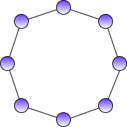
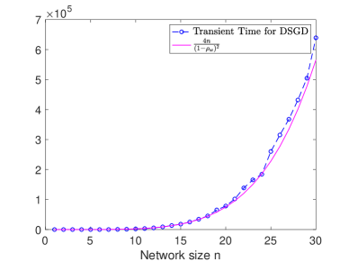
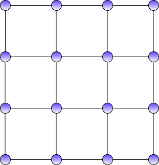
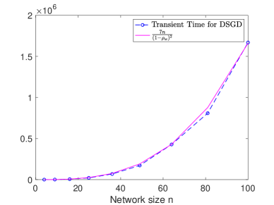
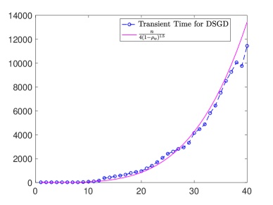
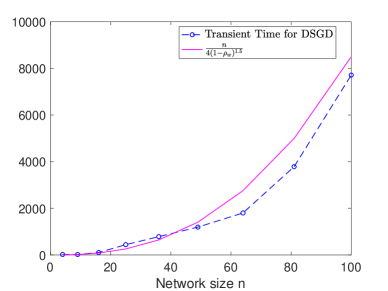
Additionally, we provide numerical experiments that demonstrate the tightness of the theoretical findings. In particular, for the ring network topology and the square grid network topology, simulations are consistent with the transient time $K_{T}=\mathcal{O}\left(\frac{n}{(1-\rho_{w})^{2}}\right)$ for solving the on-line ridge regression problem.

I-C Notation

Vectors are column vectors unless otherwise specified. Each agent $i$ holds a local copy of the decision vector denoted by $x_{i}\in\mathbb{R}^{p}$, and its value at iteration/time $k$ is written as $x_{i}(k)$. Let

$$\mathbf{x}:=[x_{1},x_{2},\ldots,x_{n}]^{\intercal}\in\mathbb{R}^{n\times p},\quad\overline{x}:=\color[rgb]{0,0,0}{\frac{1}{n}\sum_{i=1}^{n}x_{i}},$$

where $\intercal$ denotes transpose. Define an aggregate objective function

$$F(\mathbf{x}):=\sum_{i=1}^{n}f_{i}(x_{i}),$$

and let

$$\nabla F(\mathbf{x}):=\left[\nabla f_{1}(x_{1}),\nabla f_{2}(x_{2}),\ldots,\nabla f_{n}(x_{n})\right]^{\intercal}\in\mathbb{R}^{n\times p},$$

$$\bar{\nabla}F(\mathbf{x}):=\color[rgb]{0,0,0}{\frac{1}{n}\sum_{i=1}^{n}\nabla f_{i}(x_{i})}.$$

In addition, we denote

$$\boldsymbol{\xi}:=[\xi_{1},\xi_{2},\ldots,\xi_{n}]^{\intercal}\in\mathbb{R}^{n\times p},$$

$$\mathbf{g}(\mathbf{x},\boldsymbol{\xi}):=[g_{1}(x_{1},\xi_{1}),g_{2}(x_{2},\xi_{2}),\ldots,g_{n}(x_{n},\xi_{n})]^{\intercal}\in\mathbb{R}^{n\times p}.$$

In what follows we write $g_{i}(k):=g_{i}(x_{i}(k),\xi_{i}(k))$ and $\mathbf{g}(k):=\mathbf{g}(\mathbf{x}(k),\boldsymbol{\xi}(k))$ for short.

The inner product of two vectors $a,b$ is written as $\langle a,b\rangle$. For two matrices $\mathbf{A},\mathbf{B}\in\mathbb{R}^{n\times p}$, let $\langle\mathbf{A},\mathbf{B}\rangle:=\sum_{i=1}^{n}\langle A_{i},B_{i}\rangle$, where $A_{i}$ (respectively, $B_{i}$) is the $i$-th row of $\mathbf{A}$ (respectively, $\mathbf{B}$). We use $\|\cdot\|$ to denote the $2$-norm of vectors and the Frobenius norm of matrices.

A graph $\mathcal{G}=(\mathcal{N},\mathcal{E})$ has a set of vertices (nodes) $\mathcal{N}=\{1,2,\ldots,n\}$ and a set of edges connecting vertices $\mathcal{E}\subseteq\mathcal{N}\times\mathcal{N}$. Suppose agents interact in an undirected graph, i.e., $(i,j)\in\mathcal{E}$ if and only if $(j,i)\in\mathcal{E}$.

Denote the mixing matrix of agents by $\mathbf{W}=[w_{ij}]\in\mathbb{R}^{n\times n}$. Two agents $i$ and $j$ are connected if and only if $w_{ij},w_{ji}>0$ ($w_{ij}=w_{ji}=0$ otherwise). Formally, we make the following assumption on the communication among agents.

Assumption 2.

The graph $\mathcal{G}$ is undirected and connected (there exists a path between any two nodes). The mixing matrix $\mathbf{W}$ is nonnegative and doubly stochastic, i.e., $\mathbf{W}\mathbf{1}=\mathbf{1}$ and $\mathbf{1}^{\intercal}\mathbf{W}=\mathbf{1}^{\intercal}$.

From Assumption 2, we have the following contraction property of $\mathbf{W}$ (see [20]).

Lemma 1.

Let Assumption 2 hold, and let $\rho_{w}$ denote the spectral norm of the matrix $\mathbf{W}-\frac{1}{n}\mathbf{1}\mathbf{1}^{\intercal}$. Then, $\rho_{w}<1$ and

$$\|\mathbf{W}\boldsymbol{\omega}-\mathbf{1}\overline{\omega}\|\leq\rho_{w}\|\boldsymbol{\omega}-\mathbf{1}\overline{\omega}\|$$

for all $\boldsymbol{\omega}\in\mathbb{R}^{n\times p}$, where $\overline{\omega}:=\frac{1}{n}\mathbf{1}^{\intercal}\boldsymbol{\omega}$.

The rest of this paper is organized as follows. We present the DSGD algorithm and some preliminary results in Section II. In Section III we prove the sublinear convergence rate of the algorithm. Our main convergence results and a comparison with the centralized stochastic gradient method are in Section IV. Two numerical example are presented in Section V, and we conclude the paper in Section VI.

II Distributed Stochastic Gradient Descent

We consider the following DSGD method adapted from DGD and the diffusion strategy [1]: at each step $k\geq 0$, every agent $i$ independently performs the update:

$$x_{i}(k+1)=\sum_{j=1}^{n}w_{ij}\left(x_{j}(k)-\alpha_{k}g_{j}(k)\right),$$ (3)

where $\{\alpha_{k}\}$ is a sequence of non-increasing stepsizes. The particular choice of the stepsize sequence will be introduced in Section III. The initial vectors $x_{i}(0)$ are arbitrary for all $i\in{\cal N}$. We can rewrite (3) in the following compact form:

$$\mathbf{x}(k+1)=\mathbf{W}\left(\mathbf{x}(k)-\alpha_{k}\mathbf{g}(k)\right).$$ (4)

Throughout the paper, we make the following standing assumption regarding the objective functions $f_{i}$. These assumptions are satisfied for many machine learning problems, such as linear regression, smooth support vector machine (SVM), logistic regression, and softmax regression.

Assumption 3.

Each $f_{i}:\mathbb{R}^{p}\rightarrow\mathbb{R}$ is $\mu$-strongly convex with $L$-Lipschitz continuous gradients, i.e., for any $x,x^{\prime}\in\mathbb{R}^{p}$,

$$\begin{split}&\langle\nabla f_{i}(x)-\nabla f_{i}(x^{\prime}),x-x^{\prime}\rangle\geq\mu\|x-x^{\prime}\|^{2},\\ &\|\nabla f_{i}(x)-\nabla f_{i}(x^{\prime})\|\leq L\|x-x^{\prime}\|.\end{split}$$ (5)

Under Assumption 3, Problem (1) has a unique optimal solution $x_{*}\in\mathbb{R}^{p}$, and the following result holds (see [20] Lemma 10).

Lemma 2.

For any $x\in\mathbb{R}^{p}$ and $\alpha\in(0,2/L)$, we have

$$\|x-\alpha\nabla f(x)-x_{*}\|\leq\lambda\|x-x_{*}\|,$$

where $\lambda=\max(|1-\alpha\mu|,|1-\alpha L|)$.

Denote $\overline{g}(k):=\frac{1}{n}\sum_{i=1}^{n}g_{i}(k)$. The following two results are useful for our analysis.

Lemma 3.

Under Assumptions 1 and 3, for all $k\geq 0$,

$$\mathbb{E}\left[\left\|\overline{g}(k)-\bar{\nabla}F(\mathbf{x}(k))\right\|^{2}\mid\mathcal{F}(k)\right]\\ \leq\frac{2ML^{2}}{n^{2}}\|\mathbf{x}(k)-\mathbf{1}x_{*}^{\intercal}\|^{2}+\frac{\bar{M}}{n},$$

where

$$\bar{M}:=\frac{2M\sum_{i=1}^{n}\|\nabla f_{i}(x_{*})\|^{2}}{n}+\sigma^{2}.$$

Proof.

By definitions of $\overline{g}(k)$, $\bar{\nabla}F(\mathbf{x}(k))$ and Assumption 1, we have

$$\mathbb{E}\left[\left\|\overline{g}(k)-\bar{\nabla}F(\mathbf{x}(k))\right\|^{2}\right]$$

$$\quad=\color[rgb]{0,0,0}{\mathbb{E}\left[\left\|\frac{1}{n}\sum_{i=1}^{n}g_{i}(k)-\frac{1}{n}\sum_{i=1}^{n}\nabla f_{i}(x_{i}(k))\right\|^{2}\right]}$$

$$\quad=\frac{1}{n^{2}}\sum_{i=1}^{n}\mathbb{E}\left[\|g_{i}(k)-\nabla f_{i}(x_{i}(k))\|^{2}\right]$$

$$\quad\leq\frac{\sigma^{2}}{n}{\color[rgb]{0,0,0}{+}\frac{M\sum_{i=1}^{n}\|\nabla f_{i}(x_{i}(k))\|^{2}}{n^{2}}}.$$

Notice that $\|\nabla f_{i}(x_{i}(k))\|^{2}=\|\nabla f_{i}(x_{i}(k))-\nabla f_{i}(x_{*})+\nabla f_{i}(x_{*})\|^{2}\leq 2\|\nabla f_{i}(x_{i}(k))-\nabla f_{i}(x_{*})\|^{2}+2\|\nabla f_{i}(x_{*})\|^{2}\leq 2L^{2}\|x_{i}(k)-x_{*}\|^{2}+2\|\nabla f_{i}(x_{*})\|^{2}$ from Assumption 3. We have

$$\mathbb{E}\left[\left\|\overline{g}(k)-\bar{\nabla}F(\mathbf{x}(k))\right\|^{2}\right]\leq\frac{2ML^{2}}{n^{2}}\|\mathbf{x}(k)-\mathbf{1}x_{*}^{\intercal}\|^{2}\\ +\frac{1}{n}\left(\frac{2M\sum_{i=1}^{n}\|\nabla f_{i}(x_{*})\|^{2}}{n}+\sigma^{2}\right).$$

∎

Lemma 4.

Under Assumption 3, for all $k\geq 0$,

$$\left\|\nabla f(\overline{x}(k))-\bar{\nabla}F(\mathbf{x}(k))\right\|\leq\frac{L}{\sqrt{n}}\|\mathbf{x}(k)-\mathbf{1}\overline{x}(k)^{\intercal}\|.$$ (6)

Proof.

By definition,

$$\left\|\nabla f(\overline{x}(k))-\bar{\nabla}F(\mathbf{x}(k))\right\|$$

$$\quad=\left\|\frac{1}{n}\sum_{i=1}^{n}\nabla f_{i}(\overline{x}(k))-\frac{1}{n}\sum_{i=1}^{n}\nabla f_{i}(x_{i}(k))\right\|$$

(Assumption 3) $$\quad\leq\frac{L}{n}\sum_{i=1}^{n}\|\overline{x}(k)-x_{i}(k)\|$$

$$\quad\leq\frac{L}{\sqrt{n}}\|\mathbf{x}(k)-\mathbf{1}\overline{x}(k)^{\intercal}\|,$$

where the last relation follows from Hölder’s inequality. ∎

II-A Preliminary Results

In this section, we present some preliminary results concerning $\mathbb{E}[\|\overline{x}(k)-x_{*}\|^{2}]$ (expected optimization error) and $\mathbb{E}[\|\mathbf{x}(k)-\mathbf{1}\overline{x}(k)^{\intercal}\|^{2}]$ (expected consensus error). Specifically, we bound the two terms by linear combinations of their values in the last iteration.

For ease of presentation, for all $k$ we denote

$$U(k):=\mathbb{E}\left[\|\overline{x}(k)-x_{*}\|^{2}\right],\,V(k):=\mathbb{E}[\|\mathbf{x}(k)-\mathbf{1}\overline{x}(k)^{\intercal}\|^{2}].$$

In the lemma below, we bound the optimization error $U(k+1)$ by several error terms at iteration $k$, including the consensus error $V(k)$. It serves as a starting point for the follow-up analysis.

Lemma 5.

Suppose Assumptions 1-3 hold. Under Algorithm (4), supposing $\alpha_{k}\leq\frac{1}{L}$, we have

$$U(k+1)\leq(1-\alpha_{k}\mu)^{2}U(k)$$

$$\quad+\frac{2\alpha_{k}L}{\sqrt{n}}(1-\alpha_{k}\mu)\mathbb{E}[\|\overline{x}(k)-x_{*}\|\|\mathbf{x}(k)-\mathbf{1}\overline{x}(k)^{\intercal}\|]$$

$$\quad+\frac{\alpha_{k}^{2}L^{2}}{n}V(k)+\alpha_{k}^{2}\color[rgb]{0,0,0}{\left(\frac{2ML^{2}}{n^{2}}\mathbb{E}[\|\mathbf{x}(k)-\mathbf{1}x_{*}^{\intercal}\|^{2}]+\frac{\bar{M}}{n}\right)}.$$ (7)

Proof.

By the definitions of $\bar{x}(k)$, $\overline{g}(k)$ and relation (4), we have $\overline{x}(k+1)=\overline{x}(k)-\alpha_{k}\overline{g}(k).$ Hence,

$$\begin{array}[]{ll}&\|\overline{x}(k+1)-x_{*}\|^{2}=\left\|\overline{x}(k)-\alpha_{k}\overline{g}(k)-x_{*}\right\|^{2}\\ =&\left\|\overline{x}(k)-\alpha_{k}\bar{\nabla}F(\mathbf{x}(k))-x_{*}+\alpha_{k}\bar{\nabla}F(\mathbf{x}(k))-\alpha_{k}\overline{g}(k)\right\|^{2}\\ =&\|\overline{x}(k)-\alpha_{k}\bar{\nabla}F(\mathbf{x}(k))-x_{*}\|^{2}+\alpha_{k}^{2}\|\bar{\nabla}F(\mathbf{x}(k))-\overline{g}(k)\|^{2}\\ &+2\alpha_{k}\langle\overline{x}(k)-\alpha_{k}\bar{\nabla}F(\mathbf{x}(k))-x_{*},\bar{\nabla}F(\mathbf{x}(k))-\overline{g}(k)\rangle.\end{array}$$

Noting that $\mathbb{E}[\overline{g}(k)\mid\mathbf{x}(k)]=\bar{\nabla}F(\mathbf{x}(k))$ and $\mathbb{E}[\left\|\overline{g}(k)-\bar{\nabla}F(\mathbf{x}(k))\right\|^{2}\mid\mathcal{F}(k)]\leq\color[rgb]{0,0,0}{\frac{2ML^{2}}{n^{2}}\|\mathbf{x}(k)-\mathbf{1}x_{*}^{\intercal}\|^{2}+\frac{\bar{M}}{n}}$ from Lemma 3, we obtain

$$\mathbb{E}[\|\overline{x}(k+1)-x_{*}\|^{2}\mid\mathcal{F}(k)]\leq\|\overline{x}(k)-\alpha_{k}\bar{\nabla}F(\mathbf{x}(k))-x_{*}\|^{2}\\ +\alpha_{k}^{2}\left(\color[rgb]{0,0,0}{\frac{2ML^{2}}{n^{2}}\|\mathbf{x}(k)-\mathbf{1}x_{*}^{\intercal}\|^{2}+\frac{\bar{M}}{n}}\right).$$ (8)

We next bound the first term on the right-hand-side of (8).

$$\|\overline{x}(k)-\alpha_{k}\bar{\nabla}F(\mathbf{x}(k))-x_{*}\|^{2}$$

$$= \|\overline{x}(k)-\alpha_{k}\nabla f(\overline{x}(k))-x_{*}+\alpha_{k}\nabla f(\overline{x}(k))-\alpha_{k}\bar{\nabla}F(\mathbf{x}(k))\|^{2}$$

$$\leq \|\overline{x}(k)-\alpha_{k}\nabla f(\overline{x}(k))-x_{*}\|^{2}$$

$$+2\alpha_{k}\|\overline{x}(k)-\alpha_{k}\nabla f(\overline{x}(k))-x_{*}\|\|\nabla f(\overline{x}(k))-\bar{\nabla}F(\mathbf{x}(k))\|$$

$$+\alpha_{k}^{2}\|\nabla f(\overline{x}(k))-\bar{\nabla}F(\mathbf{x}(k))\|^{2},$$

where we used the Cauchy-Schwarz inequality. By Lemma 3,

$$\begin{array}[]{l}\|\nabla f(\overline{x}(k))-\bar{\nabla}F(\mathbf{x}(k))\|^{2}\leq\frac{L^{2}}{n}\|\mathbf{x}(k)-\mathbf{1}\overline{x}(k)^{\intercal}\|^{2}.\end{array}$$

Since $\alpha_{k}\leq\frac{1}{L}$, in light of Lemma 2,

$$\begin{array}[]{l}\left\|\overline{x}(k)-\alpha_{k}\nabla f(\overline{x}(k))-x_{*}\right\|^{2}\leq(1-\alpha_{k}\mu)^{2}\left\|\overline{x}(k)-x_{*}\right\|^{2}.\end{array}$$

Then we have

$$\|\overline{x}(k)-\alpha_{k}\bar{\nabla}F(\mathbf{x}(k))-x_{*}\|^{2}\leq(1-\alpha_{k}\mu)^{2}\|\overline{x}(k)-x_{*}\|^{2}\\ +\frac{2\alpha_{k}L}{\sqrt{n}}(1-\alpha_{k}\mu)\|\overline{x}(k)-x_{*}\|\|\mathbf{x}(k)-\mathbf{1}\overline{x}(k)^{\intercal}\|\\ +\frac{\alpha_{k}^{2}L^{2}}{n}\|\mathbf{x}(k)-\mathbf{1}\overline{x}(k)^{\intercal}\|^{2}.$$ (9)

In light of relation (9), taking full expectation on both sides of relation (8) yields the result. ∎

The next result is a corollary of Lemma 5 with an additional condition on the stepsize $\alpha_{k}$. We are able to remove the cross term in relation (5) and obtain a cleaner expression, which facilitates our later analysis.

Lemma 6.

Suppose Assumptions 1-3 hold. Under Algorithm (4), supposing $\alpha_{k}\leq\min\{\frac{1}{L},\frac{1}{3\mu}\}$, then

$$U(k+1)\leq\left(1-\frac{3}{2}\alpha_{k}\mu\right)U(k)+\frac{3\alpha_{k}L^{2}}{n\mu}V(k)\\ +\alpha_{k}^{2}\left(\color[rgb]{0,0,0}{\frac{2ML^{2}}{n^{2}}\mathbb{E}[\|\mathbf{x}(k)-\mathbf{1}x_{*}^{\intercal}\|^{2}]+\frac{\bar{M}}{n}}\right).$$ (10)

Proof.

From Lemma 5,

$$U(k+1)\leq(1-\alpha_{k}\mu)^{2}U(k)+(1-\alpha_{k}\mu)^{2}cU(k)$$

$$\quad+\frac{\alpha_{k}^{2}L^{2}}{n}\frac{1}{c}V(k)+\frac{\alpha_{k}^{2}L^{2}}{n}V(k)$$

$$\quad+\alpha_{k}^{2}\left(\color[rgb]{0,0,0}{\frac{2ML^{2}}{n^{2}}\mathbb{E}[\|\mathbf{x}(k)-\mathbf{1}x_{*}^{\intercal}\|^{2}]+\frac{\bar{M}}{n}}\right)$$

$$\leq(1+c)(1-\alpha_{k}\mu)^{2}U(k)+\left(1+\frac{1}{c}\right)\frac{\alpha_{k}^{2}L^{2}}{n}V(k)$$

$$\quad+\alpha_{k}^{2}\left(\color[rgb]{0,0,0}{\frac{2ML^{2}}{n^{2}}\mathbb{E}[\|\mathbf{x}(k)-\mathbf{1}x_{*}^{\intercal}\|^{2}]+\frac{\bar{M}}{n}}\right),$$

where $c>0$ is arbitrary.

Take $c=\frac{3}{8}\alpha_{k}\mu$. Noting that $\alpha_{k}\leq\frac{1}{3\mu}$, we have $(1+c)(1-\alpha_{k}\mu)^{2}\leq 1-\frac{3}{2}\alpha_{k}\mu$, and $(1+\frac{1}{c})\alpha_{k}\leq\frac{3}{\mu}$. Thus,

$$U(k+1)\leq\left(1-\frac{3}{2}\alpha_{k}\mu\right)U(k)+\frac{3\alpha_{k}L^{2}}{n\mu}V(k)\\ +\alpha_{k}^{2}\left(\frac{2ML^{2}}{n^{2}}\mathbb{E}[\|\mathbf{x}(k)-\mathbf{1}x_{*}^{\intercal}\|^{2}]+\frac{\bar{M}}{n}\right).$$

∎

Since the consensus error term $V(k)$ plays a key role in the statements of Lemma 5 and Lemma 6, we present the following lemma that bounds $V(k+1)$.

Lemma 7.

Suppose Assumptions 1-3 hold. Under Algorithm (4), for all $k\geq 0$,

$$V(k+1)\leq\frac{\left(3+\rho_{w}^{2}\right)}{4}V(k)+\alpha_{k}^{2}\rho_{w}^{2}n\sigma^{2}$$

$$\quad+2\alpha_{k}^{2}\rho_{w}^{2}\left(\frac{3}{1-\rho_{w}^{2}}+M\right)\left(L^{2}\mathbb{E}[\|\mathbf{x}(k)-\mathbf{1}x_{*}^{\intercal}\|^{2}]\right.$$

$$\quad\left.+\|\nabla F(\mathbf{1}x_{*}^{\intercal})\|^{2}\right).$$ (11)

Proof.

From relation (4),

$$\mathbf{x}(k+1)-\mathbf{1}\overline{x}(k+1)^{\intercal}$$

$$=\mathbf{W}\left(\mathbf{x}(k)-\alpha_{k}\mathbf{g}(k)\right)-\mathbf{1}(\overline{x}(k)-\alpha_{k}\overline{g}(k))$$

$$=\left(\mathbf{W}-\frac{\mathbf{1}\mathbf{1}^{\intercal}}{n}\right)\left[(\mathbf{x}(k)-\mathbf{1}\overline{x}(k)^{\intercal})-\alpha_{k}(\mathbf{g}(k)-\mathbf{1}\overline{g}(k)^{\intercal})\right],$$

we have

$$\|\mathbf{x}(k+1)-\mathbf{1}\overline{x}(k+1)^{\intercal}\|^{2}$$

$$\leq\rho_{w}^{2}\left\|(\mathbf{x}(k)-\mathbf{1}\overline{x}(k)^{\intercal})-\alpha_{k}(\mathbf{g}(k)-\mathbf{1}\overline{g}(k)^{\intercal})\right\|^{2}$$

$$=\rho_{w}^{2}\left[\left\|\mathbf{x}(k)-\mathbf{1}\overline{x}(k)^{\intercal}\right\|^{2}+\alpha_{k}^{2}\|\mathbf{g}(k)-\mathbf{1}\overline{g}(k)^{\intercal}\|^{2}\right.$$

$$\quad-2\alpha_{k}\langle\mathbf{x}(k)-\mathbf{1}\overline{x}(k)^{\intercal},\mathbf{g}(k)-\mathbf{1}\overline{g}(k)^{\intercal}\rangle\Big{]}.$$

Since $\mathbb{E}[\mathbf{g}(k)\mid\mathcal{F}(k)]=\nabla F(\mathbf{x}(k))$ and $\mathbb{E}[\overline{g}(k)\mid\mathcal{F}(k)]=\bar{\nabla}F(\mathbf{x}(k))$,

$$\mathbb{E}\left[\langle\mathbf{x}(k)-\mathbf{1}\overline{x}(k)^{\intercal},\mathbf{g}(k)-\mathbf{1}\overline{g}(k)^{\intercal}\rangle\mid\mathcal{F}(k)\right]\\ =\langle\mathbf{x}(k)-\mathbf{1}\overline{x}(k)^{\intercal},\nabla F(\mathbf{x}(k))-\mathbf{1}\bar{\nabla}F(\mathbf{x}(k))\rangle,$$

and

$$\mathbb{E}[\|\mathbf{g}(k)-\mathbf{1}\overline{g}(k)^{\intercal}\|^{2}\mid\mathcal{F}(k)]$$

$$=\mathbb{E}[\|\nabla F(\mathbf{x}(k))-\mathbf{1}\bar{\nabla}F(\mathbf{x}(k))-\nabla F(\mathbf{x}(k))+\mathbf{1}\bar{\nabla}F(\mathbf{x}(k))$$

$$\quad+\mathbf{g}(k)-\mathbf{1}\overline{g}(k)^{\intercal}\|^{2}\mid\mathcal{F}(k)]$$

$$=\|\nabla F(\mathbf{x}(k))-\mathbf{1}\bar{\nabla}F(\mathbf{x}(k))\|^{2}$$

$$\quad+\mathbb{E}[\|\nabla F(\mathbf{x}(k))-\mathbf{g}(k)-$$

$$\quad\quad\quad\quad(\mathbf{1}\bar{\nabla}F(\mathbf{x}(k))-\mathbf{1}\overline{g}(k)^{\intercal})\|^{2}\mid\mathcal{F}(k)]$$

$$\leq\|\nabla F(\mathbf{x}(k))-\mathbf{1}\bar{\nabla}F(\mathbf{x}(k))\|^{2}$$

$$\quad+\mathbb{E}[\|\nabla F(\mathbf{x}(k))-\mathbf{g}(k)\|^{2}\mid\mathcal{F}(k)]$$

$$\leq\|\nabla F(\mathbf{x}(k))-\mathbf{1}\bar{\nabla}F(\mathbf{x}(k))\|^{2}+n\sigma^{2}+\color[rgb]{0,0,0}{M\|\nabla F(\mathbf{x}(k))\|^{2}},$$

where the last inequality follows from Assumption 1. Therefore (assuming $\rho_{w}>0$),

$$\frac{1}{\rho_{w}^{2}}\mathbb{E}[\|\mathbf{x}(k+1)-\mathbf{1}\overline{x}(k+1)^{\intercal}\|^{2}\mid\mathcal{F}(k)]$$

$$\leq\left\|\mathbf{x}(k)-\mathbf{1}\overline{x}(k)^{\intercal}\right\|^{2}+\alpha_{k}^{2}\|\nabla F(\mathbf{x}(k))-\mathbf{1}\bar{\nabla}F(\mathbf{x}(k))\|^{2}$$

$$\quad+\alpha_{k}^{2}\left(n\sigma^{2}+\color[rgb]{0,0,0}{M\|\nabla F(\mathbf{x}(k))\|^{2}}\right)$$

$$\quad-2\alpha_{k}\langle\mathbf{x}(k)-\mathbf{1}\overline{x}(k)^{\intercal},\nabla F(\mathbf{x}(k))-\mathbf{1}\bar{\nabla}F(\mathbf{x}(k))\rangle$$

$$\leq\left\|\mathbf{x}(k)-\mathbf{1}\overline{x}(k)^{\intercal}\right\|^{2}+\alpha_{k}^{2}{\color[rgb]{0,0,0}{(}1+M)}\|\nabla F(\mathbf{x}(k))\|^{2}+\alpha_{k}^{2}n\sigma^{2}$$

$$\quad+2\alpha_{k}\left\|\mathbf{x}(k)-\mathbf{1}\overline{x}(k)^{\intercal}\right\|\left\|\nabla F(\mathbf{x}(k))\right\|$$

$${\color[rgb]{0,0,0}{\leq}(1+c)\left\|\mathbf{x}(k)-\mathbf{1}\overline{x}(k)^{\intercal}\right\|^{2}+\alpha_{k}^{2}(1+M)\|\nabla F(\mathbf{x}(k))\|^{2}}$$

$$\quad{\color[rgb]{0,0,0}{+}\alpha_{k}^{2}n\sigma^{2}+\frac{\alpha_{k}^{2}}{c}\left\|\nabla F(\mathbf{x}(k))\right\|^{2}},$$

where $c>0$ is arbitrary. Letting $c=\frac{1-\rho_{w}^{2}}{2}$ and noting that by Assumption 3,

$$\|\nabla F(\mathbf{x}(k))\|^{2}\leq 2\|\nabla F(\mathbf{x}(k))-\nabla F(\mathbf{1}x_{*}^{\intercal})\|^{2}+2\|\nabla F(\mathbf{1}x_{*}^{\intercal})\|^{2}$$

$$\leq 2L^{2}\|\mathbf{x}(k)-\mathbf{1}x_{*}^{\intercal}\|^{2}+2\|\nabla F(\mathbf{1}x_{*}^{\intercal})\|^{2},$$

we have

$$\frac{1}{\rho_{w}^{2}}\mathbb{E}[\|\mathbf{x}(k+1)-\mathbf{1}\overline{x}(k+1)^{\intercal}\|^{2}\mid\mathcal{F}(k)]-\alpha_{k}^{2}n\sigma^{2}$$

$$\leq\left(\frac{3-\rho_{w}^{2}}{2}\right)\left\|\mathbf{x}(k)-\mathbf{1}\overline{x}(k)^{\intercal}\right\|^{2}$$

$$\quad+2\alpha_{k}^{2}\left(\frac{3}{1-\rho_{w}^{2}}+M\right)(L^{2}\|\mathbf{x}(k)-\mathbf{1}x_{*}^{\intercal}\|^{2}+\|\nabla F(\mathbf{1}x_{*}^{\intercal})\|^{2}).$$

Notice that $\rho_{w}^{2}\left(\frac{3-\rho_{w}^{2}}{2}\right)\leq\frac{(3+\rho_{w}^{2})}{4}$. In light of Lemma 8, taking full expectation on both sides of the above inequality leads to

$$\mathbb{E}[\|\mathbf{x}(k+1)-\mathbf{1}\overline{x}(k+1)^{\intercal}\|^{2}]-\alpha_{k}^{2}\rho_{w}^{2}n\sigma^{2}$$

$$\leq\frac{(3+\rho_{w}^{2})}{4}\mathbb{E}[\left\|\mathbf{x}(k)-\mathbf{1}\overline{x}(k)^{\intercal}\right\|^{2}]$$

$$\quad+2\alpha_{k}^{2}\rho_{w}^{2}\left(\frac{3}{1-\rho_{w}^{2}}+M\right)\left(L^{2}\mathbb{E}[\|\mathbf{x}(k)-\mathbf{1}x_{*}^{\intercal}\|^{2}]\right.$$

$$\quad\left.+\|\nabla F(\mathbf{1}x_{*}^{\intercal})\|^{2}\right).$$

∎

III Analysis

We are now ready to derive some preliminary convergence results for Algorithm (4). First, we provide a uniform bound on the iterates generated by Algorithm (4) (in expectation) for all $k\geq 0$. Then based on the lemmas established in Section II-A, we prove the sublinear convergence rate for Algorithm (4), i.e., $U(k)=\mathcal{O}(\frac{1}{k})$ and $V(k)=\mathcal{O}(\frac{1}{k^{2}})$. These results provide the foundation for our main convergence theorems in Section IV.

From now on we consider the following stepsize policy:

$$\alpha_{k}:=\frac{\theta}{\mu(k+K)},\quad\forall k,$$ (12)

where constant $\theta>1$, and

$$K:=\left\lceil\frac{2\theta{\color[rgb]{0,0,0}{(}1+M)}L^{2}}{\mu^{2}}\right\rceil,$$ (13)

with $\lceil\cdot\rceil$ denoting the ceiling function.

III-A Uniform Bound

We first derive a uniform bound on the iterates generated by Algorithm (4) (in expectation) for all $k\geq 0$. Such a result is helpful for bounding the error terms on the right hand sides of (5), (10) and (7).

Lemma 8.

Suppose Assumptions 1-3 hold. Under Algorithm (4) with stepsize policy (12), for all $k\geq 0$, we have

$$\mathbb{E}[\|\mathbf{x}(k)-\mathbf{1}x_{*}^{\intercal}\|^{2}]\leq\hat{X}\\ :=\max\left\{\|\mathbf{x}(0)-\mathbf{1}x_{*}^{\intercal}\|^{2},\,\frac{9\|\nabla F(\mathbf{1}x_{*}^{\intercal})\|^{2}}{\mu^{2}}+\frac{n\sigma^{2}}{{\color[rgb]{0,0,0}{(}1+M)}L^{2}}\right\}.$$ (14)

Proof.

The following arguments are inspired by those in [35].

First, we bound $\mathbb{E}\left[\|x_{i}(k)-\alpha_{k}g_{i}(k)\|^{2}\right]$ for all $i\in\mathcal{N}$ and $k\geq 0$. By Assumption 1,

$$\mathbb{E}\left[\|x_{i}(k)-\alpha_{k}g_{i}(k)\|^{2}\mid\mathcal{F}(k)\right]$$

$$=\|x_{i}(k)-\alpha_{k}\nabla f_{i}(x_{i}(k))\|^{2}$$

$$\quad+\alpha_{k}^{2}\mathbb{E}\left[\|\nabla f_{i}(x_{i}(k))-g_{i}(k)\|^{2}\mid\mathcal{F}(k)\right]$$

$$\leq\|x_{i}(k)\|^{2}-2\alpha_{k}\langle\nabla f_{i}(x_{i}(k)),x_{i}(k)\rangle+\alpha_{k}^{2}\|\nabla f_{i}(x_{i}(k))\|^{2}$$

$$\quad+\alpha_{k}^{2}(\sigma^{2}{\color[rgb]{0,0,0}{+}M\|\nabla f_{i}(x_{i}(k))\|^{2}}).$$

From the strong convexity and Lipschitz continuity of $f_{i}$, we know that

$$\langle\nabla f_{i}(x_{i}(k)),x_{i}(k)\rangle$$

$$=\langle\nabla f_{i}(x_{i}(k))-\nabla f_{i}(0),x_{i}(k)-0\rangle+\langle\nabla f_{i}(0),x_{i}(k)\rangle$$

$$\geq\mu\|x_{i}(k)\|^{2}+\langle\nabla f_{i}(0),x_{i}(k)\rangle,$$

and

$$\|\nabla f_{i}(x_{i}(k))\|^{2}=\|\nabla f_{i}(x_{i}(k))-\nabla f_{i}(0)+\nabla f_{i}(0)\|^{2}\\ \leq 2L^{2}\|x_{i}(k)\|^{2}+2\|\nabla f_{i}(0)\|^{2}.$$

Hence,

$$\begin{split}&\mathbb{E}\left[\|x_{i}(k)-\alpha_{k}g_{i}(k)\|^{2}\mid\mathcal{F}(k)\right]\\ &\leq\|x_{i}(k)\|^{2}-2\alpha_{k}\left[\mu\|x_{i}(k)\|^{2}+\langle\nabla f_{i}(0),x_{i}(k)\rangle\right]\\ &\quad+2\alpha_{k}^{2}{\color[rgb]{0,0,0}{(}1+M)}\left(L^{2}\|x_{i}(k)\|^{2}+\|\nabla f_{i}(0)\|^{2}\right)+\alpha_{k}^{2}\sigma^{2}\\ &\leq\|x_{i}(k)\|^{2}-2\alpha_{k}\mu\|x_{i}(k)\|^{2}+2\alpha_{k}\|\nabla f_{i}(0)\|\|x_{i}(k)\|\\ &\quad+2\alpha_{k}^{2}{\color[rgb]{0,0,0}{(}1+M)}\left(L^{2}\|x_{i}(k)\|^{2}+\|\nabla f_{i}(0)\|^{2}\right)+\alpha_{k}^{2}\sigma^{2}\\ &\leq[1-2\alpha_{k}\mu+2\alpha_{k}^{2}{\color[rgb]{0,0,0}{(}1+M)}L^{2}]\|x_{i}(k)\|^{2}\\ &\quad+2\alpha_{k}\|\nabla f_{i}(0)\|\|x_{i}(k)\|+\alpha_{k}^{2}\left[2{\color[rgb]{0,0,0}{(}1+M)}\|\nabla f_{i}(0)\|^{2}+\sigma^{2}\right].\end{split}$$

Taking full expectation on both sides, it follows that

$$\begin{split}&\mathbb{E}\left[\|x_{i}(k)-\alpha_{k}g_{i}(k)\|^{2}\right]\\ &\leq[1-2\alpha_{k}\mu+2\alpha_{k}^{2}{\color[rgb]{0,0,0}{(}1+M)}L^{2}]\mathbb{E}[\|x_{i}(k)\|^{2}]\\ &\quad+2\alpha_{k}\|\nabla f_{i}(0)\|\sqrt{\mathbb{E}[\|x_{i}(k)\|^{2}]}\\ &\quad+\alpha_{k}^{2}\left[2{\color[rgb]{0,0,0}{(}1+M)}\|\nabla f_{i}(0)\|^{2}+\sigma^{2}\right].\end{split}$$

From the definition of $K$ in (13), $\alpha_{k}\leq\frac{\mu}{2{\color[rgb]{0,0,0}{(}1+M)}L^{2}}$ for all $k\geq 0$. Hence,

$$\begin{split}&\mathbb{E}\left[\|x_{i}(k)-\alpha_{k}g_{i}(k)\|^{2}\right]\\ &\leq(1-\alpha_{k}\mu)\mathbb{E}[\|x_{i}(k)\|^{2}]+2\alpha_{k}\|\nabla f_{i}(0)\|\sqrt{\mathbb{E}[\|x_{i}(k)\|^{2}]}\\ &\quad+\alpha_{k}^{2}\left[2{\color[rgb]{0,0,0}{(}1+M)}\|\nabla f_{i}(0)\|^{2}+\sigma^{2}\right]\\ &\leq\mathbb{E}[\|x_{i}(k)\|^{2}]-\alpha_{k}\Big{[}\mu\mathbb{E}[\|x_{i}(k)\|^{2}]-2\|\nabla f_{i}(0)\|\sqrt{\mathbb{E}[\|x_{i}(k)\|^{2}]}\\ &\quad\left.-\frac{\mu}{2L^{2}}\left(2\|\nabla f_{i}(0)\|^{2}+\frac{\sigma^{2}}{{\color[rgb]{0,0,0}{(}1+M)}}\right)\right].\end{split}$$ (15)

Let us define the following set:

$$\mathcal{X}_{i}:=\Big{\{}q\geq 0:\mu q-2\|\nabla f_{i}(0)\|\sqrt{q}\\ \left.-\frac{\mu}{2L^{2}}\left(2\|\nabla f_{i}(0)\|^{2}+\frac{\sigma^{2}}{{\color[rgb]{0,0,0}{(}1+M)}}\right)\leq 0\right\},$$ (16)

which is non-empty and compact. If $\mathbb{E}[\|x_{i}(k)\|^{2}]\notin\mathcal{X}_{i}$, we know from inequality (15) that $\mathbb{E}\left[\|x_{i}(k)-\alpha_{k}g_{i}(k)\|^{2}\right]\leq\mathbb{E}[\|x_{i}(k)\|^{2}]$. Otherwise,

$$\begin{split}&\mathbb{E}\left[\|x_{i}(k)-\alpha_{k}g_{i}(k)\|^{2}\right]\leq\max_{q\in\mathcal{X}_{i}}\left\{q-\frac{\mu}{2{\color[rgb]{0,0,0}{(}1+M)}L^{2}}\Big{[}\mu q\right.\\ &\quad\left.\left.-2\|\nabla f_{i}(0)\|\sqrt{q}-\frac{\mu}{2L^{2}}\left(2\|\nabla f_{i}(0)\|^{2}+\frac{\sigma^{2}}{{\color[rgb]{0,0,0}{(}1+M)}}\right)\right]\right\}\\ &=\max_{q\in\mathcal{X}_{i}}\left\{\left(1-\frac{\mu^{2}}{2{\color[rgb]{0,0,0}{(}1+M)}L^{2}}\right)q+\frac{\mu}{{\color[rgb]{0,0,0}{(}1+M)}L^{2}}\|\nabla f_{i}(0)\|\sqrt{q}\right.\\ &\quad\left.+\frac{\mu^{2}}{4{\color[rgb]{0,0,0}{(}1+M)}L^{4}}\left(2\|\nabla f_{i}(0)\|^{2}+\frac{\sigma^{2}}{{\color[rgb]{0,0,0}{(}1+M)}}\right)\right\}.\end{split}$$

Define the last term above as $R_{i}$. The previous arguments imply that for all $k\geq 0$,

$$\color[rgb]{0,0,0}{\mathbb{E}\left[\|x_{i}(k)-\alpha_{k}g_{i}(k)\|^{2}\right]\leq\max\{\mathbb{E}\left[\|x_{i}(k)\|^{2}\right],R_{i}\}.}$$

Note that from relation (4),

$$\|\mathbf{x}(k+1)\|^{2}\leq\|\mathbf{W}\|^{2}\|\mathbf{x}(k)-\alpha_{k}\mathbf{g}(k)\|^{2}\\ \leq\|\mathbf{x}(k)-\alpha_{k}\mathbf{g}(k)\|^{2}.$$

We have

$$\begin{array}[]{l}\mathbb{E}[\|\mathbf{x}(k)\|^{2}]\leq\max\left\{\|\mathbf{x}(0)\|^{2},\sum_{i=1}^{n}R_{i}\right\}.\end{array}$$ (17)

We further bound $R_{i}$ as follows. From the definition of $\mathcal{X}_{i}$,

$$\max_{q\in\mathcal{X}_{i}}q\leq\linebreak[4]\frac{8\|\nabla f_{i}(0)\|^{2}}{\mu^{2}}+\frac{3\sigma^{2}}{4{\color[rgb]{0,0,0}{(}1+M)}L^{2}}.$$

Hence,

$$\begin{array}[]{l}R_{i}=\max_{q\in\mathcal{X}_{i}}\left\{q-\frac{\mu}{2{\color[rgb]{0,0,0}{(}1+M)}L^{2}}\Big{[}\mu q-2\|\nabla f_{i}(0)\|\sqrt{q}\right.\\ \quad\left.\left.-\frac{\mu}{2L^{2}}\left(2\|\nabla f_{i}(0)\|^{2}+\frac{\sigma^{2}}{{\color[rgb]{0,0,0}{(}1+M)}}\right)\right]\right\}\\ \leq\max_{q\in\mathcal{X}_{i}}q-\frac{\mu}{2{\color[rgb]{0,0,0}{(}1+M)}L^{2}}\min_{q\in\mathcal{X}_{i}}\Big{\{}\mu q-2\|\nabla f_{i}(0)\|\sqrt{q}\\ \quad\left.-\frac{\mu}{2L^{2}}\left(2\|\nabla f_{i}(0)\|^{2}+\frac{\sigma^{2}}{{\color[rgb]{0,0,0}{(}1+M)}}\right)\right\}\\ \leq\frac{8\|\nabla f_{i}(0)\|^{2}}{\mu^{2}}+\frac{3\sigma^{2}}{4{\color[rgb]{0,0,0}{(}1+M)}L^{2}}\\ \quad+\frac{\mu}{2{\color[rgb]{0,0,0}{(}1+M)}L^{2}}\left[\frac{\|\nabla f_{i}(0)\|^{2}}{\mu}+\frac{\mu}{2L^{2}}\left(2\|\nabla f_{i}(0)\|^{2}+\frac{\sigma^{2}}{{\color[rgb]{0,0,0}{(}1+M)}}\right)\right]\\ \leq\frac{9\|\nabla f_{i}(0)\|^{2}}{\mu^{2}}+\frac{\sigma^{2}}{{\color[rgb]{0,0,0}{(}1+M)}L^{2}}.\end{array}$$ (18)

In light of inequality (18), further noticing that the choice of $0$ is arbitrary in the proof of (17), we obtain the uniform bound for $\mathbb{E}[\|\mathbf{x}(k)-\mathbf{1}x_{*}^{\intercal}\|^{2}]$ in (14). ∎

The uniform bound provided in Lemma 8 is critical for deriving the sublinear convergence rates of $U(k)$ and $V(k$), as it holds for all $k\geq 0$.

III-B Sublinear Rate

With the help of Lemma 6 and Lemma 7 from Section II-A and Lemma 8, we show in Lemma 10 below that Algorithm (4) enjoys the sublinear convergence rate, i.e., $U(k)=\mathcal{O}(\frac{1}{k})$ and $V(k)=\mathcal{O}(\frac{1}{k^{2}})$. For the ease of analysis, we define two auxiliary variables:

$$\tilde{U}(k):=U(k-K),\,\tilde{V}(k):=V(k-K),\,\forall k\geq K.$$ (19)

We first derive uniform upper bounds for $U(k)$ and $V(k)$ respectively for all $k\geq 0$ based on Lemma 8. With these bounds, we are able to characterize the constants appearing in the sublinear convergence rates for $U(k)$ and $V(k)$ in Lemma 10 and Lemma 12 respectively.

Lemma 9.

Suppose Assumptions 1-3 hold. Under Algorithm (4), we have

$$U(k)\leq\frac{\hat{X}}{n},\,V(k)\leq\hat{X},\;\forall k\geq 0.$$ (20)

Proof.

By definitions of $U(k)$, $V(k)$, and Lemma 8, we have

$$U(k) =\mathbb{E}[\|\overline{x}(k)-x_{*}\|^{2}]$$

$$\leq\frac{1}{n}\mathbb{E}[\|\mathbf{x}(k)-\mathbf{1}x_{*}^{\intercal}\|^{2}]\leq\frac{\hat{X}}{n},$$

$$V(k) =\mathbb{E}[\|\mathbf{x}(k)-\mathbf{1}\overline{x}(k)^{\intercal}\|^{2}]$$

$$\leq\mathbb{E}[\|\mathbf{x}(k)-\mathbf{1}x_{*}^{\intercal}\|^{2}]\leq\hat{X}.$$

∎

Denote an auxiliary counter

$$\tilde{k}:=k+K,\quad\forall k\geq 0.$$ (21)

Our strategy is to first show that the consensus error of Algorithm (4) decays as $V(k)=\mathcal{O}(\frac{1}{k^{2}})$ based on Lemma 7, since $U(k)$ does not appear explicitly in relation (7).

Lemma 10.

Suppose Assumptions 1-3 hold. Let

$$K_{1}:=\left\lceil\max\left\{2K,\frac{16}{1-\rho_{w}^{2}}\right\}\right\rceil.$$ (22)

Under Algorithm (4) with stepsize (12), for all $k\geq K_{1}-K$, we have

$$V(k)\leq\frac{\hat{V}}{\tilde{k}^{2}},$$

where

$$\hat{V}:=\max\left\{K_{1}^{2}\hat{X},\frac{8\theta^{2}\rho_{w}^{2}c_{1}}{\mu^{2}(1-\rho_{w}^{2})}\right\},$$ (23)

with

$$c_{1}:=2\left(\frac{3}{1-\rho_{w}^{2}}+M\right)\left(L^{2}\hat{X}+\|\nabla F(\mathbf{1}x_{*}^{\intercal})\|^{2}\right)+n\sigma^{2}.$$ (24)

Proof.

From Lemma 7 and Lemma 8, for $k\geq 0$,

$$V(k+1)\leq\frac{\left(3+\rho_{w}^{2}\right)}{4}V(k)+\alpha_{k}^{2}\rho_{w}^{2}c_{1},$$ (25)

with $c_{1}$ defined in (24). From the definitions of $\alpha_{k}$ and $\tilde{V}(k)$ in (12) and (19) respectively, we know that when $k\geq K$,

$$\tilde{V}(k+1)\leq\frac{(3+\rho_{w}^{2})}{4}\tilde{V}(k)+\frac{\theta^{2}\rho_{w}^{2}c_{1}}{\mu^{2}}\left(\frac{1}{k^{2}}\right).$$

We now prove the lemma by induction. For $k=K_{1}$, we know $\tilde{V}(k)=\frac{K_{1}^{2}\tilde{V}(K_{1})}{K_{1}^{2}}\leq\frac{\hat{V}}{k^{2}}$ from Lemma 9. Now suppose $\tilde{V}(k)\leq\frac{\hat{V}}{k^{2}}$ for some $k\geq K_{1}$, then

$$\tilde{V}(k+1)\leq\frac{(3+\rho_{w}^{2})}{4}\frac{\hat{V}}{k^{2}}+\frac{\theta^{2}\rho_{w}^{2}c_{1}}{\mu^{2}}\left(\frac{1}{k^{2}}\right).$$

To show that $\tilde{V}(k+1)\leq\frac{\hat{V}}{(k+1)^{2}}$, it is sufficient to show

$$\frac{(3+\rho_{w}^{2})}{4}\frac{\hat{V}}{k^{2}}+\frac{\theta^{2}\rho_{w}^{2}c_{1}}{\mu^{2}}\left(\frac{1}{k^{2}}\right)\leq\frac{\hat{V}}{(k+1)^{2}},$$

or equivalently,

$$\hat{V}\geq\frac{\theta^{2}\rho_{w}^{2}c_{1}}{\mu^{2}}\left[\left(\frac{k}{k+1}\right)^{2}-\frac{3+\rho_{w}^{2}}{4}\right]^{-1}.$$ (26)

Since $k\geq K_{1}\geq\frac{16}{1-\rho_{w}^{2}}$, we have

$$\left(\frac{k}{k+1}\right)^{2}-\frac{3+\rho_{w}^{2}}{4}=-\frac{2}{k+1}+\frac{1}{(k+1)^{2}}+\frac{1-\rho_{w}^{2}}{4}\\ \geq\frac{1-\rho_{w}^{2}}{8}.$$

Hence relation (26) is satisfied with $\hat{V}\geq\frac{8\theta^{2}\rho_{w}^{2}c_{1}}{\mu^{2}(1-\rho_{w}^{2})}$. We then have for all $k\geq K_{1}$,

$$\tilde{V}(k)\leq\frac{1}{k^{2}}\max\left\{K_{1}^{2}\hat{X},\frac{8\theta^{2}\rho_{w}^{2}c_{1}}{\mu^{2}(1-\rho_{w}^{2})}\right\}.$$

Recalling the connection of $\tilde{V}(k)$ and $V(k)$, we conclude that $V(k)\leq\frac{\hat{V}}{\tilde{k}^{2}}$ for all $k\geq K_{1}-K$. ∎

To prove the sublinear convergence of $U(k)$, we start with a useful lemma which provides lower and upper bounds for the product of a decreasing sequence. Such products arise in the convergence proof for $U(k)$ and our main convergence results in Section IV.

Lemma 11.

For any $1<a<k$ ($a\in\mathbb{N}$) and $1<\gamma\leq a/2$,

$$\frac{a^{2\gamma}}{k^{2\gamma}}\leq\prod_{t=a}^{k-1}\left(1-\frac{\gamma}{t}\right)\leq\frac{a^{\gamma}}{k^{\gamma}}.$$

Proof.

Denote $G(k):=\prod_{t=a}^{k-1}\left(1-\frac{\gamma}{t}\right)$. We first show that $G(k)\leq\frac{a^{\gamma}}{k^{\gamma}}$. Suppose $G(k)\leq\frac{M_{1}}{k^{\gamma}}$ for some $M_{1}>0$ and $k\geq a$. Then,

$$G(k+1)=\left(1-\frac{\gamma}{k}\right)G(k)\leq\left(1-\frac{\gamma}{k}\right)\frac{M_{1}}{k^{\gamma}}\leq\frac{M_{1}}{(k+1)^{\gamma}}.$$

To see why the last inequality holds, note that $\left(\frac{k}{k+1}\right)^{\gamma}\geq 1-\frac{\gamma}{k}$. Taking $M_{1}=a^{\gamma}$, we have $G(a)=1\leq\frac{M_{1}}{a^{\gamma}}$. The desired relation then holds for all $k>a$.

Now suppose $G(k)\geq\frac{M_{2}}{k^{2\gamma}}$ for some $M_{2}>0$ and $k\geq a$. It follows that

$$G(k+1)=\left(1-\frac{\gamma}{k}\right)G(k)\geq\left(1-\frac{\gamma}{k}\right)\frac{M_{2}}{k^{2\gamma}}\geq\frac{M_{2}}{(k+1)^{2\gamma}},$$

where the last inequality follows from $\left(\frac{k}{k+1}\right)^{2\gamma}\leq 1-\frac{\gamma}{k}$ (noting that $\gamma\leq a/2\leq k/2$). Taking $M_{2}=a^{2\gamma}$, we have $G(a)=1\leq\frac{M_{2}}{a^{2\gamma}}$. The desired relation then holds for all $k>a$. ∎

In light of Lemma 6 and the other supporting lemmas, we establish the $\mathcal{O}(\frac{1}{k})$ convergence rate of $U(k)$ in the following lemma.

Lemma 12.

Suppose Assumptions 1-3 hold. Under Algorithm (4) with stepsize (12), suppose $\theta>2$. We have

$$U(k)\leq\frac{\theta^{2}{\color[rgb]{0,0,0}{c}_{2}}}{(1.5\theta-1)n\mu^{2}\tilde{k}}{\color[rgb]{0,0,0}{+}\frac{K_{1}^{1.5\theta}}{\tilde{k}^{1.5\theta}}\frac{\hat{X}}{n}}\\ \quad+\left[\frac{3\theta^{2}(1.5\theta-1){\color[rgb]{0,0,0}{c}_{2}}}{(1.5\theta-2)n\mu^{2}}+\frac{6\theta L^{2}\hat{V}}{(1.5\theta-2)n\mu^{2}}\right]\frac{1}{\tilde{k}^{2}},$$

for all $k\geq K_{1}-K$, where

$$c_{2}:=\frac{2ML^{2}}{n}\hat{X}+\bar{M}.$$ (27)

Proof.

In light of Lemma 6 and Lemma 8, for all $k\geq 0$, we have

$$U(k+1)\leq\left(1-\frac{3}{2}\alpha_{k}\mu\right)U(k)+\frac{3\alpha_{k}L^{2}}{n\mu}V(k)+\frac{\alpha_{k}^{2}{\color[rgb]{0,0,0}{c}_{2}}}{n}.$$

Recalling the definitions of $\tilde{U}(k)$ and $\tilde{V}(k)$, for all $k\geq K$,

$$\tilde{U}(k+1)\leq\left(1-\frac{3\theta}{2k}\right)\tilde{U}(k)+\frac{3\theta L^{2}}{n\mu^{2}}\frac{\tilde{V}(k)}{k}+\frac{\theta^{2}{\color[rgb]{0,0,0}{c}_{2}}}{n\mu^{2}}\frac{1}{k^{2}}.$$

Therefore,

$$\tilde{U}(k)\leq\prod_{t=K_{1}}^{k-1}\left(1-\frac{3\theta}{2t}\right)\tilde{U}(K_{1})\\ +\sum_{t=K_{1}}^{k-1}\left(\prod_{j=t+1}^{k-1}\left(1-\frac{3\theta}{2j}\right)\right)\left(\frac{\theta^{2}{\color[rgb]{0,0,0}{c}_{2}}}{n\mu^{2}}\frac{1}{t^{2}}+\frac{3\theta L^{2}}{n\mu^{2}}\frac{\tilde{V}(t)}{t}\right).$$

From Lemma 11,

$$\tilde{U}(k)\leq\frac{K_{1}^{1.5\theta}}{k^{1.5\theta}}\tilde{U}(K_{1})$$

$$\quad+\sum_{t=K_{1}}^{k-1}\frac{(t+1)^{1.5\theta}}{k^{1.5\theta}}\left(\frac{\theta^{2}{\color[rgb]{0,0,0}{c}_{2}}}{n\mu^{2}t^{2}}+\frac{3\theta L^{2}}{n\mu^{2}}\frac{\tilde{V}(t)}{t}\right)$$

$$=\frac{1}{k^{1.5\theta}}\frac{\theta^{2}{\color[rgb]{0,0,0}{c}_{2}}}{n\mu^{2}}\sum_{t=K_{1}}^{k-1}\frac{(t+1)^{1.5\theta}}{t^{2}}+\frac{K_{1}^{1.5\theta}}{k^{1.5\theta}}\tilde{U}(K_{1})$$

$$\quad+\sum_{t=K_{1}}^{k-1}\frac{(t+1)^{1.5\theta}}{k^{1.5\theta}}\frac{3\theta L^{2}}{n\mu^{2}}\frac{\tilde{V}(t)}{t}.$$

In light of Lemma 10, when $k\geq K_{1}$, $\tilde{V}(k)\leq\frac{\hat{V}}{k^{2}}$. Hence,

$$\tilde{U}(k)-\frac{1}{k^{1.5\theta}}\frac{\theta^{2}{\color[rgb]{0,0,0}{c}_{2}}}{n\mu^{2}}\sum_{t=K_{1}}^{k-1}\frac{(t+1)^{1.5\theta}}{t^{2}}-\frac{K_{1}^{1.5\theta}}{k^{1.5\theta}}\tilde{U}(K_{1})$$

$$\leq\sum_{t=K_{1}}^{k-1}\frac{(t+1)^{1.5\theta}}{k^{1.5\theta}}\frac{3\theta L^{2}}{n\mu^{2}}\frac{\hat{V}}{t^{3}}$$

$$=\frac{1}{k^{1.5\theta}}\frac{3\theta L^{2}\hat{V}}{n\mu^{2}}\sum_{t=K_{1}}^{k-1}\frac{(t+1)^{1.5\theta}}{t^{3}}.$$

However, we have for any $b>a\geq K_{1}$,

$$\sum_{a}^{b}\frac{(t+1)^{1.5\theta}}{t^{2}}$$

$$\leq\sum_{a}^{b-2}\left[\frac{(t+1)^{1.5\theta}}{(t+1)^{2}}+3\frac{(t+1)^{1.5\theta}}{(t+1)^{3}}\right]+\frac{b^{1.5\theta}}{(b-1)^{2}}$$

$$\quad+\frac{(b+1)^{1.5\theta}}{b^{2}}$$

$$\leq\int_{a}^{b}\left(t^{1.5\theta-2}+3t^{1.5\theta-3}\right)dt+\frac{2(b+1)^{1.5\theta}}{b^{2}}$$

$$\leq\frac{b^{1.5\theta-1}}{1.5\theta-1}+\frac{3b^{1.5\theta-2}}{1.5\theta-2}+3b^{1.5\theta-2},$$

where the last inequality comes from the fact that $(\frac{b+1}{b})^{1.5\theta}\leq(\frac{4\theta+1}{4\theta})^{1.5\theta}\leq\exp(\frac{3}{8})<\frac{3}{2}$ (given that $b>K_{1}\geq 4\theta$), and

$$\sum_{a}^{b}\frac{(t+1)^{1.5\theta}}{t^{3}}\leq\frac{3}{2}\sum_{a}^{b}t^{1.5\theta-3}\leq\frac{3}{2}\int_{a}^{b+1}t^{1.5\theta-3}dt$$

$$\leq\frac{3}{2}\frac{(b+1)^{1.5\theta-2}}{1.5\theta-2}\leq\frac{2b^{1.5\theta-2}}{1.5\theta-2}.$$

Hence, for all $k\geq K_{1}$,

$$\tilde{U}(k)\leq\frac{\theta^{2}{\color[rgb]{0,0,0}{c}_{2}}}{(1.5\theta-1)n\mu^{2}k}+\frac{3\theta^{2}(1.5\theta-1){\color[rgb]{0,0,0}{c}_{2}}}{(1.5\theta-2)n\mu^{2}}\frac{1}{k^{2}}\\ +\frac{K_{1}^{1.5\theta}}{k^{1.5\theta}}\tilde{U}(K_{1})+\frac{6\theta L^{2}\hat{V}}{(1.5\theta-2)n\mu^{2}}\frac{1}{k^{2}}.$$

Recalling Lemma 9 and the definition of $\tilde{U}(k)$ yields the desired result. ∎

Remark 1.

Notice that the convergence rate established in Lemma 12 is not asymptotically the same as centralized stochastic gradient descent, since the constant $c_{2}$ contains information about the initial solutions. In the next section, we will improve the convergence result and show that DSGD indeed performs as well as centralized SGD asymptotically.

IV Main Results

In this section, we perform a non-asymptotic analysis of network independence for Algorithm (4). Specifically, in Theorem 1, we show that

$$\frac{1}{n}\sum_{i=1}^{n}\mathbb{E}[\|x_{i}(k)-x_{*}\|^{2}] =\frac{\theta^{2}\color[rgb]{0,0,0}{\bar{M}}}{(2\theta-1)n\mu^{2}\tilde{k}}$$

$$+\mathcal{O}\left(\frac{1}{\sqrt{n}(1-\rho_{w})}\right)\frac{1}{\tilde{k}^{1.5}}$$

$$+\mathcal{O}\left(\frac{1}{(1-\rho_{w})^{2}}\right)\frac{1}{\tilde{k}^{2}},$$

where the first term is network independent and the second and third (higher-order) terms depends on $(1-\rho_{w})$. Then we compare the result with centralized stochastic gradient descent and show that asymptotically, the two methods have the same convergence rate $\color[rgb]{0,0,0}{\frac{\theta^{2}\color[rgb]{0,0,0}{\bar{M}}}{(2\theta-1)n\mu^{2}\tilde{k}}}$. In addition, it takes $K_{T}=\mathcal{O}\left(\frac{n}{(1-\rho_{w})^{2}}\right)$ time for Algorithm (4) to reach this asymptotic rate of convergence. Finally, we construct a “hard” optimization problem for which we show the transient time $K_{T}$ is sharp.

Our first step is to simplify the presentation of the convergence results in Lemma 10 and Lemma 12, so that we can utilize them for deriving improved convergence rates conveniently. For this purpose, we first estimate the constants $\hat{X}$, $\hat{V}$, $c_{1}$ and $c_{2}$ appearing in the two lemmas and derive their dependency on the network size $n$, the spectral gap $(1-\rho_{w})$, the summation of initial optimization errors $\sum_{i=1}^{n}\|x_{i}(0)-x_{*}\|^{2}$, and $\sum_{i=1}^{n}\|\nabla f_{i}(x_{*})\|^{2}$, where the last term can be seen as a measure of the difference among each agent’s individual cost functions.

Lemma 13.

Denote $A:=\sum_{i=1}^{n}\|x_{i}(0)-x_{*}\|^{2}$ and $B:=\sum_{i=1}^{n}\|\nabla f_{i}(x_{*})\|^{2}$. Then,

$$\hat{X}=\mathcal{O}(A+B+n),\quad c_{1}=\mathcal{O}\left(\frac{A+B+n}{1-\rho_{w}}\right),$$

$$\hat{V}=\mathcal{O}\left(\frac{A+B+n}{(1-\rho_{w})^{2}}\right),\quad c_{2}=\mathcal{O}\left(\frac{A+B+n}{n}\right).$$

Proof.

We first estimate the constant $\hat{X}$ which appears in the definition (23) for $\hat{V}$. From Lemma 8,

$$\hat{X}\leq\|\mathbf{x}(0)-\mathbf{1}x_{*}\|^{2}+\frac{9\|\nabla F(\mathbf{1}x_{*}^{\intercal})\|^{2}}{\mu^{2}}+\frac{n\sigma^{2}}{{\color[rgb]{0,0,0}{(}1+M)}L^{2}}\\ =\mathcal{O}(A+B+n).$$

From the definition of $c_{1}$ in (24),

$$c_{1}=2\left(\frac{3}{1-\rho_{w}^{2}}+M\right)\left(L^{2}\hat{X}+\|\nabla F(\mathbf{1}x_{*}^{\intercal})\|^{2}\right)+n\sigma^{2}\\ =\mathcal{O}\left(\frac{A+B+n}{1-\rho_{w}}\right).$$

Noting that $K_{1}=\mathcal{O}(\frac{1}{1-\rho_{w}})$, by definition,

$$\hat{V}=\max\left\{K_{1}^{2}\hat{X},\frac{8\theta^{2}\rho_{w}^{2}c_{1}}{\mu^{2}(1-\rho_{w}^{2})}\right\}=\mathcal{O}\left(\frac{A+B+n}{(1-\rho_{w})^{2}}\right).$$

From the definition of $c_{2}$ in (27), we have

$$c_{2}=\frac{2ML^{2}}{n}\hat{X}+\bar{M}=\mathcal{O}\left(\frac{A+B+n}{n}\right).$$

∎

In light of Lemma 13, the convergence result of $V(k)$ given in Lemma 10 can be easily simplified since $\hat{V}$ is the only constant. Regarding the optimization error $U(k)$, in light of Lemma 8, Lemma 10, Lemma 12 and Lemma 13, we have the following corollary which simplifies the presentation of the convergence result in Lemma 12.

Corollary 1.

Suppose Assumptions 1-3 hold. Under Algorithm (4) with stepsize (12) and assuming $\theta>2$, when $k\geq K_{1}-K$,

$$U(k)\leq\frac{\theta^{2}{\color[rgb]{0,0,0}{c}_{2}}}{(1.5\theta-1)n\mu^{2}\tilde{k}}+\frac{c}{\tilde{k}^{2}},$$

where

$$c=\mathcal{O}\left(\color[rgb]{0,0,0}{\frac{A+B+n}{n(1-\rho_{w})^{2}}}\right).$$

Proof.

From Theorem 12 and Lemma 13, when $k\geq K_{1}-K=\mathcal{O}(\frac{1}{1-\rho_{w}})$,

$$U(k)\leq \frac{\theta^{2}{\color[rgb]{0,0,0}{c}_{2}}}{(1.5\theta-1)n\mu^{2}\tilde{k}}{\color[rgb]{0,0,0}{+}\frac{K_{1}^{1.5\theta-2}}{\tilde{k}^{1.5\theta-2}}\frac{\hat{X}}{n}\frac{K_{1}^{2}}{\tilde{k}^{2}}}$$

$$+\left[\frac{3\theta^{2}(1.5\theta-1){\color[rgb]{0,0,0}{c}_{2}}}{(1.5\theta-2)n\mu^{2}}+\frac{6\theta L^{2}\hat{V}}{(1.5\theta-2)n\mu^{2}}\right]\frac{1}{\tilde{k}^{2}}$$

$$= \frac{\theta^{2}{\color[rgb]{0,0,0}{c}_{2}}}{(1.5\theta-1)n\mu^{2}}\frac{1}{\tilde{k}}+\mathcal{O}\left(\color[rgb]{0,0,0}{\frac{A+B+n}{n(1-\rho_{w})^{2}}}\right)\frac{1}{\tilde{k}^{2}}.$$ (28)

∎

Let $\frac{1}{n}\sum_{i=1}^{n}\mathbb{E}[\|x_{i}(k)-x_{*}\|^{2}]$, the average optimization error for each agent to measure the performance of DSGD. In the following theorem, we improve the result of Corollary 1 with further analysis and derive the main convergence result for Algorithm (4).

Theorem 1.

Suppose Assumptions 1-3 hold. Under Algorithm (4) with stepsize (12) and assuming $\theta>2$, when $k\geq K_{1}-K$,

$$\frac{1}{n}\sum_{i=1}^{n}\mathbb{E}[\|x_{i}(k)-x_{*}\|^{2}]\leq\frac{\theta^{2}\color[rgb]{0,0,0}{\bar{M}}}{(2\theta-1)n\mu^{2}\tilde{k}}\\ +\mathcal{O}\left(\color[rgb]{0,0,0}{\frac{\sqrt{A+B+n}}{n(1-\rho_{w})}}\right)\frac{1}{\tilde{k}^{1.5}}+\mathcal{O}\left(\color[rgb]{0,0,0}{\frac{A+B+n}{n(1-\rho_{w})^{2}}}\right)\frac{1}{\tilde{k}^{2}}.$$ (29)

Proof.

For $k\geq K_{1}-K$, in light of Lemma 2 and Lemma 5,

$$\begin{split}&U(k+1)\\ &\leq(1-\alpha_{k}\mu)^{2}U(k)+\frac{2\alpha_{k}L}{\sqrt{n}}\mathbb{E}[\|\overline{x}(k)-x_{*}\|\|\mathbf{x}(k)-\mathbf{1}\overline{x}(k)^{\intercal}\|]\\ &\quad+\frac{\alpha_{k}^{2}L^{2}}{n}V(k)+{\color[rgb]{0,0,0}{\alpha}_{k}^{2}\left(\frac{2ML^{2}}{n^{2}}\mathbb{E}[\|\mathbf{x}(k)-\mathbf{1}x_{*}^{\intercal}\|^{2}]+\frac{\bar{M}}{n}\right)}\\ &\leq(1-\alpha_{k}\mu)^{2}U(k)+\frac{2\alpha_{k}L}{\sqrt{n}}\sqrt{U(k)V(k)}+\frac{\alpha_{k}^{2}L^{2}}{n}V(k)\\ &\quad+{\color[rgb]{0,0,0}{\alpha}_{k}^{2}\left[\frac{2ML^{2}}{n^{2}}(nU(k)+V(k))+\frac{\bar{M}}{n}\right]}\\ &{\color[rgb]{0,0,0}{=}(1-2\alpha_{k}\mu)U(k)+\alpha_{k}^{2}\left(\mu^{2}+\frac{2ML^{2}}{n}\right)U(k)}\\ &\quad{\color[rgb]{0,0,0}{+}\frac{2\alpha_{k}L}{\sqrt{n}}\sqrt{U(k)V(k)}+\frac{\alpha_{k}^{2}L^{2}}{n}\left(1+\frac{2M}{n}\right)V(k)+\frac{\alpha_{k}^{2}\bar{M}}{n},}\end{split}$$

where the second inequality follows from the Cauchy-Schwarz inequality (see [52], page 62) and the fact that $\|\mathbf{x}(k)-\mathbf{1}x_{*}^{\intercal}\|^{2}=\|\mathbf{x}(k)-\mathbf{1}\bar{x}(k)\|^{2}+n\|\bar{x}(k)-x_{*}\|^{2}$.

Recalling the definitions of $\tilde{U}(k)$ and $\tilde{V}(k)$, when $k\geq K_{1}$,

$$\tilde{U}(k+1)\leq\left(1-\frac{2\theta}{k}\right)\tilde{U}(k)+\frac{\theta^{2}}{k^{2}}\left(1+\frac{2ML^{2}}{n\mu^{2}}\right)\tilde{U}(k)\\ +\frac{2\theta L}{\sqrt{n}\mu}\frac{\sqrt{\tilde{U}(k)\tilde{V}(k)}}{k}+\frac{\theta^{2}L^{2}}{n\mu^{2}}\left(1+\frac{2M}{n}\right)\frac{\tilde{V}(k)}{k^{2}}+\frac{\theta^{2}\bar{M}}{n\mu^{2}}\frac{1}{k^{2}}.$$

Therefore, by denoting $c_{3}:=1+\frac{2ML^{2}}{n\mu^{2}}$ and $c_{4}:=1+\frac{2M}{n}$, we have

$$\tilde{U}(k)\leq\left(\prod_{t=K_{1}}^{k-1}\left(1-\frac{2\theta}{t}\right)\right)\tilde{U}(K_{1})$$

$$\quad+\sum_{t=K_{1}}^{k-1}\left(\prod_{i=t+1}^{k-1}\left(1-\frac{2\theta}{i}\right)\right)$$

$$\quad\cdot\left(\frac{\theta^{2}\color[rgb]{0,0,0}{\bar{M}}}{n\mu^{2}t^{2}}+\frac{\theta^{2}{\color[rgb]{0,0,0}{c}_{3}}\tilde{U}(t)}{t^{2}}+\frac{2\theta L}{\sqrt{n}\mu}\frac{\sqrt{\tilde{U}(t)\tilde{V}(t)}}{t}+\frac{\theta^{2}L^{2}{\color[rgb]{0,0,0}{c}_{4}}}{n\mu^{2}}\frac{\tilde{V}(t)}{t^{2}}\right)$$

From Lemma 11,

$$\begin{split}&\tilde{U}(k)\leq\frac{K_{1}^{2\theta}}{k^{2\theta}}\tilde{U}(K_{1})+\sum_{t=K_{1}}^{k-1}\frac{(t+1)^{2\theta}}{k^{2\theta}}\left(\frac{\theta^{2}\color[rgb]{0,0,0}{\bar{M}}}{n\mu^{2}t^{2}}+\frac{\theta^{2}{\color[rgb]{0,0,0}{c}_{3}}\tilde{U}(t)}{t^{2}}\right.\\ &\quad\left.+\frac{2\theta L}{\sqrt{n}\mu}\frac{\sqrt{\tilde{U}(t)\tilde{V}(t)}}{t}+\frac{\theta^{2}L^{2}{\color[rgb]{0,0,0}{c}_{4}}}{n\mu^{2}}\frac{\tilde{V}(t)}{t^{2}}\right)\\ &=\frac{1}{k^{2\theta}}\frac{\theta^{2}\color[rgb]{0,0,0}{\bar{M}}}{n\mu^{2}}\sum_{t=K_{1}}^{k-1}\frac{(t+1)^{2\theta}}{t^{2}}+\frac{K_{1}^{2\theta}}{k^{2\theta}}\tilde{U}(K_{1})\\ &\quad+\sum_{t=K_{1}}^{k-1}\frac{(t+1)^{2\theta}}{k^{2\theta}}\left(\frac{\theta^{2}{\color[rgb]{0,0,0}{c}_{3}}\tilde{U}(t)}{t^{2}}+\frac{2\theta L}{\sqrt{n}\mu}\frac{\sqrt{\tilde{U}(t)\tilde{V}(t)}}{t}\right.\\ &\quad\left.+\frac{\theta^{2}L^{2}{\color[rgb]{0,0,0}{c}_{4}}}{n\mu^{2}}\frac{\tilde{V}(t)}{t^{2}}\right).\end{split}$$

Hence, by Corollary 1,

$$\begin{split}&\tilde{U}(k)-\frac{1}{k^{2\theta}}\frac{\theta^{2}\color[rgb]{0,0,0}{\bar{M}}}{n\mu^{2}}\sum_{t=K_{1}}^{k-1}\frac{(t+1)^{2\theta}}{t^{2}}-\frac{K_{1}^{2\theta}}{k^{2\theta}}\tilde{U}(K_{1})\\ &\leq\frac{\theta^{2}\color[rgb]{0,0,0}{c_{3}}}{k^{2\theta}}\sum_{t=K_{1}}^{k-1}\frac{(t+1)^{2\theta}}{t^{2}}\left[\frac{\theta^{2}{\color[rgb]{0,0,0}{c}_{2}}}{(1.5\theta-1)n\mu^{2}t}+\frac{c}{t^{2}}\right]\\ &\quad+\frac{1}{k^{2\theta}}\frac{2\theta L}{\sqrt{n}\mu}\sum_{t=K_{1}}^{k-1}\frac{(t+1)^{2\theta}}{t}\sqrt{\frac{\theta^{2}{\color[rgb]{0,0,0}{c}_{2}}}{(1.5\theta-1)n\mu^{2}}\frac{1}{t}+\frac{c}{t^{2}}}\sqrt{\frac{\hat{V}}{t^{2}}}\\ &\quad+\frac{1}{k^{2\theta}}\frac{\theta^{2}L^{2}{\color[rgb]{0,0,0}{c}_{4}}}{n\mu^{2}}\sum_{t=K_{1}}^{k-1}\frac{(t+1)^{2\theta}}{t^{2}}\frac{\hat{V}}{t^{2}}.\end{split}$$

Since

$$\sqrt{\frac{\theta^{2}{\color[rgb]{0,0,0}{c}_{2}}}{(1.5\theta-1)n\mu^{2}}\frac{1}{t}+\frac{c}{t^{2}}}\sqrt{\frac{\hat{V}}{t^{2}}}\leq\sqrt{\frac{\theta^{2}{\color[rgb]{0,0,0}{c}_{2}}\hat{V}}{(1.5\theta-1)n\mu^{2}}\frac{1}{t^{3}}}+\frac{\sqrt{c\hat{V}}}{t^{2}},$$

we have

$$\begin{split}&\tilde{U}(k)-\frac{1}{k^{2\theta}}\frac{\theta^{2}\color[rgb]{0,0,0}{\bar{M}}}{n\mu^{2}}\sum_{t=K_{1}}^{k-1}\frac{(t+1)^{2\theta}}{t^{2}}-\frac{K_{1}^{2\theta}}{k^{2\theta}}\tilde{U}(K_{1})\\ &\leq\frac{\theta^{2}{\color[rgb]{0,0,0}{c}_{3}}}{k^{2\theta}}\sum_{t=K_{1}}^{k-1}\frac{(t+1)^{2\theta}}{t^{2}}\left[\frac{\theta^{2}{\color[rgb]{0,0,0}{c}_{2}}}{(1.5\theta-1)n\mu^{2}}\frac{1}{t}+\frac{c}{t^{2}}\right]\\ &\quad+\frac{1}{k^{2\theta}}\frac{2\theta L}{\sqrt{n}\mu}\sum_{t=K_{1}}^{k-1}\frac{(t+1)^{2\theta}}{t}\left(\sqrt{\frac{\theta^{2}{\color[rgb]{0,0,0}{c}_{2}}\hat{V}}{(1.5\theta-1)n\mu^{2}}\frac{1}{t^{3}}}+\frac{\sqrt{c\hat{V}}}{t^{2}}\right)\\ &\quad+\frac{1}{k^{2\theta}}\frac{\theta^{2}L^{2}{\color[rgb]{0,0,0}{c}_{4}}\hat{V}}{n\mu^{2}}\sum_{t=K_{1}}^{k-1}\frac{(t+1)^{2\theta}}{t^{4}}\\ &=\frac{1}{k^{2\theta}}\left(\frac{2\theta^{2}L\sigma\sqrt{{\color[rgb]{0,0,0}{c}_{2}}\hat{V}}}{\sqrt{1.5\theta-1}n\mu^{2}}\right)\sum_{t=K_{1}}^{k-1}\frac{(t+1)^{2\theta}}{t^{2.5}}\\ &\quad+\frac{1}{k^{2\theta}}\left(\frac{\theta^{4}{\color[rgb]{0,0,0}{c}_{3}c_{2}}}{(1.5\theta-1)n\mu^{2}}+\frac{2\theta L\sqrt{c\hat{V}}}{\sqrt{n}\mu}\right)\sum_{t=K_{1}}^{k-1}\frac{(t+1)^{2\theta}}{t^{3}}\\ &\quad+\frac{1}{k^{2\theta}}\left(\theta^{2}{\color[rgb]{0,0,0}{c}_{3}}c+\frac{\theta^{2}L^{2}{\color[rgb]{0,0,0}{c}_{4}}\hat{V}}{n\mu^{2}}\right)\sum_{t=K_{1}}^{k-1}\frac{(t+1)^{2\theta}}{t^{4}}.\end{split}$$

Notice that $c_{2}=\mathcal{O}(\frac{A+B+n}{n})$ and $c_{3},c_{4}=\mathcal{O}(1)$. Following a discussion similar to those in the proofs for Theorem 12 and Corollary 1, we have

$$\begin{split}\tilde{U}(k)\leq&\frac{\theta^{2}\color[rgb]{0,0,0}{\bar{M}}}{(2\theta-1)n\mu^{2}k}+\mathcal{O}\left(\color[rgb]{0,0,0}{\frac{\sqrt{A+B+n}}{n(1-\rho_{w})}}\right)\frac{1}{k^{1.5}}\\ &+\mathcal{O}\left(\color[rgb]{0,0,0}{\frac{A+B+n}{n(1-\rho_{w})^{2}}}\right)\frac{1}{k^{2}}+\mathcal{O}\left(\color[rgb]{0,0,0}{\frac{A+B+n}{n(1-\rho_{w})^{2}}}\right)\frac{1}{k^{3}}\\ &+\mathcal{O}\left(\color[rgb]{0,0,0}{\frac{A+B+n}{n(1-\rho_{w})^{2\theta}}}\right)\frac{1}{k^{2\theta}}\\ =&\frac{\theta^{2}\color[rgb]{0,0,0}{\bar{M}}}{(2\theta-1)n\mu^{2}k}+\mathcal{O}\left(\color[rgb]{0,0,0}{\frac{\sqrt{A+B+n}}{n(1-\rho_{w})}}\right)\frac{1}{k^{1.5}}\\ &+\mathcal{O}\left(\color[rgb]{0,0,0}{\frac{A+B+n}{n(1-\rho_{w})^{2}}}\right)\frac{1}{k^{2}}.\end{split}$$

Noting that

$$\frac{1}{n}\sum_{i=1}^{n}\mathbb{E}[\|x_{i}(k)-x_{*}\|^{2}]$$

$$=\mathbb{E}[\|\bar{x}(k)-x_{*}\|^{2}]+\frac{1}{n}\sum_{i=1}^{n}\mathbb{E}[\|x_{i}(k)-\bar{x}\|^{2}]$$

$$=U(k)+\frac{V(k)}{n},$$

and $U(k)=\tilde{U}(k+K)$, in light of the bound on $V(k)$ in Lemma 10 and the estimate of $\hat{V}$ in Lemma 13, we obtain the desired result. ∎

IV-A Comparison with Centralized Implementation

We compare the performance of DSGD and centralized stochastic gradient descent (SGD) stated below:

$$x(k+1)=x(k)-\alpha_{k}\tilde{g}(k),$$ (30)

where $\alpha_{k}:=\frac{\theta}{\mu k}$ ($\theta>1$) and $\tilde{g}(k):=\frac{1}{n}\sum_{i=1}^{n}g(x(k),\xi_{i}(k))$.

First, we derive the convergence rate for SGD which matches the optimal rate for such stochastic gradient methods (see [29, 53]). Our result relies on an analysis different from the literature that considered a compact feasible set and uniformly bounded stochastic gradients in expectation.

Theorem 2.

Under the centralized stochastic gradient descent of (30), suppose $k\geq K_{2}:=\left\lceil\frac{\theta L}{\mu}\right\rceil$. We have

$$\mathbb{E}[\|x(k)-x_{*}\|^{2}]\leq\frac{\theta^{2}\color[rgb]{0,0,0}{\bar{M}}}{(2\theta-1)n\mu^{2}k}+\mathcal{O}\left(\frac{1}{n}\right)\frac{1}{k^{2}}.$$

Proof.

Noting that $\alpha_{k}\leq 1/L$ when $k\geq K_{2}$, we have from Lemma 3 that

$$\begin{split}&\mathbb{E}[\|x(k+1)-x_{*}\|^{2}\mid\mathcal{F}(k)]\\ &=\mathbb{E}[\|x(k)-\alpha_{k}\tilde{g}(k)-x_{*}\|^{2}\mid\mathcal{F}(k)]\\ &=\|x(k)-\alpha_{k}\nabla f(x(k))-x_{*}\|^{2}+\alpha_{k}^{2}\mathbb{E}[\|\nabla f(x(k))-\tilde{g}(k)\|^{2}]\\ &\leq(1-\alpha_{k}\mu)^{2}\|x(k)-x_{*}\|^{2}\\ &\quad+\alpha_{k}^{2}\color[rgb]{0,0,0}{\left(\frac{2ML^{2}}{n}\|x(k)-x_{*}\|^{2}+\frac{\bar{M}}{n}\right)}\\ &=\left(1-\frac{2\theta}{k}\right)\|x(k)-x_{*}\|^{2}\\ &\quad+\theta^{2}\left(1{\color[rgb]{0,0,0}{+}\frac{2ML^{2}}{n\mu^{2}}}\right)\|x(k)-x_{*}\|^{2}\frac{1}{k^{2}}+\frac{\theta^{2}\color[rgb]{0,0,0}{\bar{M}}}{n\mu^{2}}\frac{1}{k^{2}}.\end{split}$$ (31)

It can be shown first that $\mathbb{E}[\|x(k)-x_{*}\|^{2}]\leq\frac{c_{5}}{k}$ for $k\geq K_{2}$, where $c_{5}=\mathcal{O}(\frac{1}{n})$. Denote $\bar{c}_{5}:=(1+\frac{2ML^{2}}{n\mu^{2}})c_{5}$. Then from relation (31), when $k\geq K_{2}$,

$$\begin{split}\mathbb{E}[\|x(k)-x_{*}\|^{2}]\leq\left(\prod_{t=K_{2}}^{k-1}\left(1-\frac{2\theta}{t}\right)\right)\mathbb{E}[\|x(K_{2})-x_{*}\|^{2}]\\ +\sum_{t=K_{2}}^{k-1}\left(\prod_{i=t+1}^{k-1}\left(1-\frac{2\theta}{i}\right)\right)\left(\frac{\theta^{2}\color[rgb]{0,0,0}{\bar{M}}}{n\mu^{2}t^{2}}+\frac{\theta^{2}\color[rgb]{0,0,0}{\bar{c}_{5}}}{t^{3}}\right).\end{split}$$

From Lemma 11,

$$\begin{split}&\mathbb{E}[\|x(k)-x_{*}\|^{2}]\leq\frac{K_{2}^{2\theta}}{k^{2\theta}}\mathbb{E}[\|x(K_{2})-x_{*}\|^{2}]\\ &\quad+\sum_{t=K_{2}}^{k-1}\frac{(t+1)^{2\theta}}{k^{2\theta}}\left(\frac{\theta^{2}\color[rgb]{0,0,0}{\bar{M}}}{n\mu^{2}t^{2}}+\frac{\theta^{2}\color[rgb]{0,0,0}{\bar{c}_{5}}}{t^{3}}\right)\\ &=\frac{1}{k^{2\theta}}\frac{\theta^{2}\color[rgb]{0,0,0}{\bar{M}}}{n\mu^{2}}\sum_{t=K_{2}}^{k-1}\frac{(t+1)^{2\theta}}{t^{2}}+\frac{K_{2}^{2\theta}}{k^{2\theta}}\mathbb{E}[\|x(K_{2})-x_{*}\|^{2}]\\ &\quad+\frac{\theta^{2}\color[rgb]{0,0,0}{\bar{c}_{5}}}{k^{2\theta}}\sum_{t=K_{2}}^{k-1}\frac{(t+1)^{2\theta}}{t^{3}}\\ &=\frac{\theta^{2}\color[rgb]{0,0,0}{\bar{M}}}{(2\theta-1)n\mu^{2}k}+\mathcal{O}\left(\frac{1}{n}\right)\frac{1}{k^{2}}.\end{split}$$

∎

Comparing the results of Theorem 1 and Theorem 2, we can see that asymptotically, DSGD and SGD have the same convergence rate $\frac{\theta^{2}\color[rgb]{0,0,0}{\bar{M}}}{(2\theta-1)n\mu^{2}k}$. The next corollary identifies the time needed for DSGD to achieve this rate.

Corollary 2 (Transient Time).

Suppose Assumptions 1-3 hold. Assume in addition that $\sum_{i=1}^{n}\|x_{i}(0)-x_{*}\|^{2}=\mathcal{O}(n)$ and $\sum_{i=1}^{n}\|\nabla f_{i}(x_{*})\|^{2}=\mathcal{O}(n)$. It takes $K_{T}=\mathcal{O}\left(\frac{n}{(1-\rho_{w})^{2}}\right)$ time for Algorithm (4) to reach the asymptotic rate of convergence, i.e., when $k\geq K_{T}$, we have $\frac{1}{n}\sum_{i=1}^{n}\mathbb{E}[\|x_{i}(k)\linebreak[3]-x_{*}\|^{2}]\leq\frac{\theta^{2}\color[rgb]{0,0,0}{\bar{M}}}{(2\theta-1)n\mu^{2}k}\mathcal{O}(1)$.

Proof.

From (29),

$$\frac{1}{n}\sum_{i=1}^{n}\mathbb{E}[\|x_{i}(k)-x_{*}\|^{2}]\leq\frac{\theta^{2}\color[rgb]{0,0,0}{\bar{M}}}{(2\theta-1)n\mu^{2}k}\\ \cdot\left[1+\mathcal{O}\left(\frac{\sqrt{n}}{(1-\rho_{w})}\right)\frac{1}{k^{0.5}}+\mathcal{O}\left(\frac{n}{(1-\rho_{w})^{2}}\right)\frac{1}{k}\right].$$

Let $K_{T}$ be such that

$$\mathcal{O}\left(\frac{\sqrt{n}}{(1-\rho_{w})}\right)\frac{1}{K_{T}^{0.5}}+\mathcal{O}\left(\frac{n}{(1-\rho_{w})^{2}}\right)\frac{1}{K_{T}}=\mathcal{O}(1).$$

We then obtain that

$$K_{T}=\mathcal{O}\left(\frac{n}{(1-\rho_{w})^{2}}\right).$$

∎

Remark 2.

By assuming the additional conditions $\sum_{i=1}^{n}\|x_{i}(0)-x_{*}\|^{2}=\mathcal{O}(n)$ and $\sum_{i=1}^{n}\|\nabla f_{i}(x_{*})\|^{2}=\mathcal{O}(n)$, motivated by the observation that each of these expression is the sum of $n$ terms, we obtain a cleaner expression of the transient time. In general, we would obtain $K_{T}=\mathcal{O}\left(\frac{A+B+n}{(1-\rho_{w})^{2}}\right)$.

Remark 3.

For general connected networks such as line graphs, if we adopt the Lazy Metropolis rule for choosing the weights $[w_{ij}]$ (see [54]), then $\frac{1}{1-\rho_{w}}=\mathcal{O}(n^{2})$, and hence $K_{T}=\mathcal{O}(n^{5})$. The transient time can be improved for networks with special structures. For example, $\frac{1}{1-\rho_{w}}$ is constant with high probability for a random Erdős-Rényi random graph, and consequently $K_{T}=\mathcal{O}(n)$ on such a graph.

The next theorem states that the transient time for DSGD to reach the asymptotic convergence rate is lower bounded by $\Omega\left(\frac{n}{(1-\rho_{w})^{2}}\right)$, that is, under Assumptions 1-3 and assuming $\sum_{i=1}^{n}\|x_{i}(0)-x_{*}\|^{2}=\mathcal{O}(n)$ and $\sum_{i=1}^{n}\|\nabla f_{i}(x_{*})\|^{2}=\mathcal{O}(n)$, there exists an optimization problem whose transient time under DSGD is lower bounded by $\Omega\left(\frac{n}{(1-\rho_{w})^{2}}\right)$. This implies the result in Corollary 2 is sharp and can not be improved in general.

Theorem 3.

Suppose Assumptions 1-3 hold. Assume in addition that $\sum_{i=1}^{n}\|x_{i}(0)-x_{*}\|^{2}=\mathcal{O}(n)$ and $\sum_{i=1}^{n}\|\nabla f_{i}(x_{*})\|^{2}=\mathcal{O}(n)$. Then there exists a $\rho_{0}\in(0,1)$ such that if $\rho_{w}\geq\rho_{0}$, then the time needed for DSGD to reach the asymptotic convergence rate is lower bounded by $\Omega\left(\frac{n}{(1-\rho_{w})^{2}}\right)$.

Proof.

We construct a “hard” optimization to prove the claimed result, inspired by [31]. Consider quadratic objective functions $f_{i}(x):=\frac{1}{2}\|x-x_{i}^{*}\|^{2}$, where $x,x_{i}^{*}\in\mathbb{R}$. The optimal solution to Problem (1) is given by $x_{*}=\frac{1}{n}\sum_{i=1}^{n}x_{i}^{*}$. The DSGD algorithm implements:

$$\mathbf{x}(k+1)=\mathbf{W}\left(\mathbf{x}(k)-\alpha_{k}(\mathbf{x}(k)-\mathbf{x}_{*})+\alpha_{k}\mathbf{n}(k)\right),$$ (32)

where $\mathbf{x}_{*}:=[x_{1}^{*},x_{2}^{*},\ldots,x_{n}^{*}]^{\intercal}$, and $\mathbf{n}(k)$ denotes the vector of gradient noise terms. From (12), we use stepsize $\alpha_{k}=\frac{\theta}{k+K}$ ($\theta>2$), where $K=\lceil 2\theta\rceil$ since $\mu=L=1$. We rewrite (32) as

$$\mathbf{x}(k+1)=(1-\alpha_{k})\mathbf{W}\mathbf{x}(k)+\alpha_{k}\mathbf{W}\mathbf{x}_{*}+\alpha_{k}\mathbf{W}\mathbf{n}(k).$$

It follows that

$$\mathbf{x}(k+1)-\mathbf{1}\overline{x}(k+1)^{\intercal}=(1-\alpha_{k})\mathbf{W}(\mathbf{x}(k)-\mathbf{1}\overline{x}(k)^{\intercal})\\ +\alpha_{k}\mathbf{W}(\mathbf{x}_{*}-\mathbf{1}x_{*})+\alpha_{k}\mathbf{W}(\mathbf{n}(k)-\mathbf{1}\overline{n}(k)).$$

By induction, we have for all $k>0$,

$$\begin{split}\mathbf{x}(k)-\mathbf{1}\overline{x}(k)^{\intercal}=&\left(\prod_{t=0}^{k-1}(1-\alpha_{t})\right)\mathbf{W}^{k}(\mathbf{x}(0)-\mathbf{1}\overline{x}(0))\\ &+\sum_{t=0}^{k-1}\left[\left(\prod_{j=t+1}^{k-1}(1-\alpha_{j})\right)\alpha_{t}\mathbf{W}^{k-t}\right]\\ &\cdot\left[(\mathbf{x}_{*}-\mathbf{1}x_{*})+(\mathbf{n}(t)-\mathbf{1}\overline{n}(t))\right].\end{split}$$ (33)

Assume that: (i) the matrix $\mathbf{W}$ is symmetric; (ii) $\mathbf{W}\mathbf{x}_{*}=\rho_{w}\mathbf{x}_{*}$, i.e., $\mathbf{x}_{*}$ is an eigenvector of $\mathbf{W}$ w.r.t. eigenvalue $\rho_{w}$ (hence $x_{*}=\frac{1}{n}\mathbf{1}^{\intercal}\mathbf{x}_{*}=0$); (iii) $\|\nabla F(\mathbf{1}x_{*}^{\intercal})\|^{2}=\|\mathbf{1}x_{*}-\mathbf{x}_{*}\|^{2}=\|\mathbf{x}_{*}\|^{2}=\Omega(n)$; (iv) $\mathbf{x}(0)=\mathbf{x}_{*}$. Then $\overline{x}(0)=x_{*}=0$, and from relation (33) it follows

$$\mathbf{x}(k)-\mathbf{1}\overline{x}(k)^{\intercal}=\left(\prod_{t=0}^{k-1}(1-\alpha_{t})\right)\rho_{w}^{k}\mathbf{x}_{*}\\ +\sum_{t=0}^{k-1}\left[\left(\prod_{j=t+1}^{k-1}(1-\alpha_{j})\right)\alpha_{t}\rho_{w}^{k-t}\right]\mathbf{x}_{*}+\epsilon(k),$$ (34)

where $\epsilon(k)$ captures the random perturbation caused by gradient noise that has mean zero. Therefore,

$$\mathbb{E}[\|\mathbf{x}(k)-\mathbf{1}\overline{x}(k)^{\intercal}\|^{2}]\geq\\ \left\|\sum_{t=0}^{k-1}\left[\left(\prod_{j=t+1}^{k-1}(1-\alpha_{j})\right)\alpha_{t}\rho_{w}^{k-t}\right]\mathbf{x}_{*}\right\|^{2}.$$

Recalling the definition $V(k)=\mathbb{E}[\|\mathbf{x}(k)-\mathbf{1}\overline{x}(k)^{\intercal}\|^{2}$ and $\tilde{V}(k)=V(k-K)$, and noticing that $\alpha_{k}=\frac{\theta}{k+K}$, we have

$$\tilde{V}(k)\geq \left\{\sum_{t=K}^{k-1}\left[\left(\prod_{j=t+1}^{k-1}\left(1-\frac{\theta}{j}\right)\right)\frac{\theta}{t}\rho_{w}^{k-t}\right]\right\}^{2}\|\mathbf{x}_{*}\|^{2}$$

$$\geq \left\{\sum_{t=K}^{k-1}\left[\frac{(t+1)^{2\theta}}{k^{2\theta}}\frac{\theta}{t}\rho_{w}^{k-t}\right]\right\}^{2}\|\mathbf{x}_{*}\|^{2},$$

where we invoked Lemma 11 for the second inequality. Then,

$$\tilde{V}(k) \geq\left[\frac{\theta\rho_{w}^{k}}{k^{2\theta}}\sum_{t=K}^{k-1}\frac{(t+1)^{2\theta-1}}{\rho_{w}^{t}}\right]^{2}\|\mathbf{x}_{*}\|^{2}$$

$$\geq\left[\frac{\theta\rho_{w}^{k}}{k^{2\theta}}\int_{t=K-1}^{k-1}\frac{(t+1)^{2\theta-1}}{\rho_{w}^{t}}dt\right]^{2}\|\mathbf{x}_{*}\|^{2}.$$ (35)

Note that when $k\geq\frac{4\theta}{(-\ln\rho_{w})}$,

$$\int_{t=K-1}^{k-1}\frac{(t+1)^{2\theta-1}}{\rho_{w}^{t}}dt\geq\frac{2}{3}\left.\frac{(t+1)^{2\theta-1}}{(-\ln\rho_{w})\rho_{w}^{t}}\right|_{t=K-1}^{k-1}\\ =\frac{2k^{2\theta-1}}{3(-\ln\rho_{w})\rho_{w}^{k-1}}-\frac{2K^{2\theta-1}}{3(-\ln\rho_{w})\rho_{w}^{K-1}}\geq\frac{k^{2\theta-1}}{2(-\ln\rho_{w})\rho_{w}^{k-1}}.$$

From (IV-A),

$$\tilde{V}(k)\geq\left[\frac{\theta\rho_{w}}{2(-\ln\rho_{w})k}\right]^{2}\|\mathbf{x}_{*}\|^{2}=\Omega\left(\frac{n}{(1-\rho_{w})^{2}}\right)\frac{1}{k^{2}},$$

where the equality is obtained from the Taylor expansion of $\ln\rho_{w}$ when $\rho_{w}\rightarrow 1$. Since

$$\frac{1}{n}\sum_{i=1}^{n}\mathbb{E}[\|x_{i}(k)-x_{*}\|^{2}]=U(k)+\frac{V(k)}{n}\geq\Omega\left(\frac{1}{(1-\rho_{w})^{2}}\right)\frac{1}{k^{2}},$$

setting this to be at most $\frac{\color[rgb]{0,0,0}{\bar{M}}}{nk}$, we obtain that the transient time for DSGD to reach the asymptotic convergence rate is lower bounded by $\Omega\left(\frac{n}{(1-\rho_{w})^{2}}\right)$, based on an argument similar to that of Corollary 2. ∎

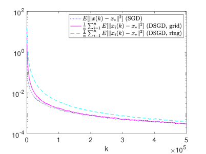
V Numerical Examples

In this section, we provide two numerical example to verify and complement our theoretical findings.

V-A Ridge Regression

Consider the on-line ridge regression problem, i.e.,

$$\min_{x\in\mathbb{R}^{p}}f(x)=\frac{1}{n}\sum_{i=1}^{n}f_{i}(x)\left(=\mathbb{E}_{u_{i},v_{i}}\left[\left(u_{i}^{\intercal}x-v_{i}\right)^{2}+\rho\|x\|^{2}\right]\right),$$ (36)

where $\rho>0$ is a penalty parameter. Each agent $i$ collects data samples in the form of $(u_{i},v_{i})$ continuously where $u_{i}\in\mathbb{R}^{p}$ represent the features and $v_{i}\in\mathbb{R}$ are the observed outputs. Assume each $u_{i}\in[-0.5,0.5]^{p}$ is uniformly distributed, and $v_{i}$ is drawn according to $v_{i}=u_{i}^{\intercal}\tilde{x}_{i}+\varepsilon_{i}$, where $\tilde{x}_{i}$ are predefined parameters evenly located in $[0,10]^{p}$, and $\varepsilon_{i}$ are independent Gaussian random variables (noise) with mean $0$ and variance $0.01$. Given a pair $(u_{i},v_{i})$, agent $i$ can compute an estimated (unbiased) gradient of $f_{i}(x)$: $g_{i}(x,u_{i},v_{i})=2(u_{i}^{\intercal}x-v_{i})u_{i}+2\rho x$. Problem (36) has a unique solution $x_{*}$ given by

$$x_{*}=\left(\sum_{i=1}^{n}\mathbb{E}_{u_{i}}[u_{i}u_{i}^{\intercal}]+n\rho\mathbf{I}\right)^{-1}\sum_{i=1}^{n}\mathbb{E}_{u_{i}}[u_{i}u_{i}^{\intercal}]\tilde{x}_{i}\\ =\frac{1}{3}\left(\frac{1}{3}+\rho\right)^{-1}\frac{1}{n}\sum_{i=1}^{n}\tilde{x}_{i}.$$ (37)

Suppose $p=10$ and $\rho=1$. We compare the performance of DSGD (3) and the centralized implementation (30) for solving problem (36) with the same stepsize policy $\alpha_{k}=20/(k+20),\forall k$, and the same initial solutions: $x_{i}(0)=\mathbf{0},\ \forall i$, (DSGD) and $x(0)=\mathbf{0}$ (SGD). It can be seen from (37) and the definition of $\tilde{x}_{i}$ that $\sum_{i=1}^{n}\|x_{i}(0)-x_{*}\|^{2}=\mathcal{O}(n)$. Moreover, $\nabla f_{i}(x_{*})=2\mathbb{E}_{u_{i},v_{i}}\left[(u_{i}^{\intercal}x_{*}-v_{i})u_{i}\right]+2\rho x_{*}=2\mathbb{E}_{u_{i}}[u_{i}u_{i}^{\intercal}](x_{*}-\tilde{x}_{i})+2\rho x_{*}=\frac{2}{3}(x_{*}-\tilde{x}_{i})+2\rho x_{*}$. Therefore, we have $\sum_{i=1}^{n}\|\nabla f_{i}(x_{*})\|^{2}=\mathcal{O}(n)$.

In Fig. 1, we provide an illustration example that compares the performance of DSGD and SGD, assuming $n=25$. For DSGD, we consider two different network topologies: ring network topology as shown in Fig. 2(a) and square grid network topology as shown in Fig. 2(a). For both network topologies, we use Metropolis weights for constructing the maxing matrix $\mathbf{W}$ (see [55]). It can be seen that DSGD performs asymptotically as well as SGD, while the time it takes for DSGD to catch up with SGD depends on the network topology. For grid networks which are better connected than rings, the corresponding transient time is shorter.

Figure 1: The performance comparison between DSGD and SGD for online Ridge regression ($n=25$). The results are averaged over $200$ Monte Carlo simulation.

To further verify the conclusions of Corollary 2 and Theorem 3, we define the transient time for DSGD as $\inf\{k:\frac{1}{n}\sum_{i=1}^{n}\mathbb{E}[\|x_{i}(k)-x_{*}\|^{2}]\leq 2\mathbb{E}[\|x(k)-x_{*}\|^{2}]\}$. For DSGD, we first assume a ring network topology and plot the transient times for DSGD and $\frac{4n}{(1-\rho_{w})^{2}}$ as a function of the network size $n$ in Fig. 2(b). We then consider a square grid network topology as shown in Fig. 2(a) and plot the transient times for DSGD and $\frac{7n}{(1-\rho_{w})^{2}}$ in Fig. 2 (b). It can be seen that the two curves in Fig. 2(b) and Fig. 3(b) are close to each other, respectively. This verifies the sharpness of Corollary 2.

(a) Ring network topology.

(b) Transient times for the ring network topology.

Figure 2: Comparison of the transient times for DSGD and $\frac{4n}{(1-\rho_{w})^{2}}$ as a function of the network size $n$ for the ring network topology. The expected errors are approximated by averaging over $200$ simulation results.

(a) Square grid network topology.

(b) Transient times for the square grid network topology.

Figure 3: Comparison of the transient times for DSGD and $\frac{7n}{(1-\rho_{w})^{2}}$ as a function of the network size $n$ for the square grid network topology ($n=4,9,16,25,36,49,64,81,100$). The expected errors are approximated by averaging over $200$ simulation results.

V-B Logistic Regression

Consider the problem of classification on the MNIST dataset of handwritten digits (http://yann.lecun.com/exdb/mnist/). In particular, we classify digits $1$ and $2$ using logistic regression. There are $12700$ data points in total where each data point is a pair $(u,v)$ with $u\in\mathbb{R}^{785}$ being the image input and $v\in\{0,1\}$ being the label.

Suppose each agent $i\in\mathcal{N}$ possesses a distinct local dataset $\mathcal{S}_{i}$ that is randomly taken from the database. To apply logistic regression for classification, we solve the following optimization problem based on all the agents’ local datasets:

$$\min_{x\in\mathbb{R}^{785}}f(x)=\frac{1}{n}\sum_{i=1}^{n}f_{i}(x),$$ (38)

where

$$f_{i}(x):=\frac{1}{|\mathcal{S}_{i}|}\sum_{j\in\mathcal{S}_{i}}\left[\log(1+\exp(-x^{\intercal}u_{j}))+(1-v_{j})x^{\intercal}u_{j}\right]\\ +\frac{\lambda}{2}\|x\|^{2},$$

where $\lambda$ is the regularization parameter. Given any solution $x$, agent $i$ is able to compute an unbiased estimate of $\nabla f_{i}(x)$ using one (or a minibatch of) randomly chosen data point $(u_{i},v_{i})$ from $\mathcal{S}_{i}$, that is,

$$g_{i}(x,u_{i},v_{i})=\frac{-u_{j}}{1+\exp(x^{\intercal}u_{j})}+(1-v_{j})u_{j}+\lambda x.$$

In the experiments, suppose each local dataset $\mathcal{S}_{i}$ contains $50$ data points, and $\lambda=1$. At each iteration of the DSGD algorithm, agent $i$ computes a stochastic gradient of $f_{i}(x_{i}(k))$ with one randomly chosen data point from $\mathcal{S}_{i}$. We compare the performance of DSGD (3) and centralized SGD (30) for solving problem (38) with the same stepsize policy $\alpha_{k}=6/(k+20),\forall k$, and the same initial solutions: $x_{i}(0)=\mathbf{0},\ \forall i$, (DSGD) and $x(0)=\mathbf{0}$ (SGD). It can be numerically verified that $\sum_{i=1}^{n}\|x_{i}(0)-x_{*}\|^{2}=\mathcal{O}(n)$ and $\sum_{i=1}^{n}\|\nabla f_{i}(x_{*})\|^{2}=\mathcal{O}(n)$.

The transient time for DSGD is defined in the same way as in the ridge regression example. In Fig. 4 and Fig. 5, we plot the transient times for DSGD as a function of the network size $n$ for ring and grid networks, respectively. We find that the curves are close to $\frac{n}{4(1-\rho_{w})^{1.5}}$, rather than a multiple of $\frac{n}{(1-\rho_{w})^{2}}$, implying that the experimental results are better than the theoretically derived worst-case performance given in Corollary 2. Hence in practice, the performance of the DSGD algorithm depends on the specific problem instances and can be better than the worst-case situation in terms of transient times.

Figure 4: Comparison of the transient times for DSGD and $\frac{n}{4(1-\rho_{w})^{1.5}}$ as a function of the network size $n$ for the ring network topology. The expected errors are approximated by averaging over $200$ simulation results.

Figure 5: Comparison of the transient times for DSGD and $\frac{n}{4(1-\rho_{w})^{1.5}}$ as a function of the network size $n$ for the grid network topology ($n=4,9,16,25,36,49,64,81,100$). The expected errors are approximated by averaging over $200$ simulation results.

VI Conclusions

This paper is devoted to the non-asymptotic analysis of network independence for the distributed stochastic gradient descent (DSGD) method. We show that the algorithm asymptotically achieves the optimal network independent convergence rate compared to SGD, and identify the non-asymptotic convergence rate as a function of characteristics of the objective functions and the network. In addition, we compute the time needed for DSGD to reach its asymptotic rate of convergence and prove the sharpness of the obtained result. Future work will consider more general problems such as nonconvex objectives and constrained optimization.

Shi Pu is currently an assistant professor in the School of Data and Decision Science, The Chinese University of Hong Kong, Shenzhen, China. He is also affiliated with Shenzhen Research Institute of Big Data. He received a B.S. Degree from Peking University, in 2012, and a Ph.D. Degree in Systems Engineering from the University of Virginia, in 2016. He was a postdoctoral associate at the University of Florida, from 2016 to 2017, a postdoctoral scholar at Arizona State University, from 2017 to 2018, and a postdoctoral associate at Boston University, from 2018 to 2019. His research interests include distributed optimization, network science, machine learning, and game theory.

Alex Olshevsky received the B.S. degrees in applied mathematics and electrical engineering from Georgia Tech and the Ph.D. degree in EECS from MIT. He is currently an Associate Professor at the ECE department at Boston University. Dr. Olshevsky is a recipient of the NSF CAREER Award, the AFOSR Young Investigator Award, the INFORMS Prize for the best paper on the interface of operations research and computer science, a SIAM Award for annual paper from the SIAM Journal on Control and Optimization chosen to be reprinted in SIAM Review, and an IMIA award for best paper on clinical informatics.

Ioannis Ch. Paschalidis (M’96–SM’06–F’14) received a Ph.D. in EECS from the Massachusetts Institute of Technology, Cambridge, MA, USA, in 1996. He is a Professor and Data Science Fellow at Boston University, Boston, MA and the Director of the Center for Information and Systems Engineering. His research interests lie in the fields of systems and control, networks, applied probability, optimization, operations research, computational biology, and medical informatics. He is a recipient of the NSF CAREER award and several best paper awards. During 2013–2019 he was the founding Editor-in-Chief of the IEEE Transactions on Control of Network Systems.

References

• [1] J. Chen and A. H. Sayed, “Diffusion adaptation strategies for distributed optimization and learning over networks,” IEEE Transactions on Signal Processing, vol. 60, no. 8, pp. 4289–4305, 2012.
• [2] A. I. Forrester, A. Sóbester, and A. J. Keane, “Multi-fidelity optimization via surrogate modelling,” Proceedings of the Royal Society of London A, vol. 463, no. 2088, pp. 3251–3269, 2007.
• [3] A. Nedić, A. Olshevsky, and C. A. Uribe, “Fast convergence rates for distributed non-bayesian learning,” IEEE Transactions on Automatic Control, vol. 62, no. 11, pp. 5538–5553, 2017.
• [4] K. Cohen, A. Nedić, and R. Srikant, “On projected stochastic gradient descent algorithm with weighted averaging for least squares regression,” IEEE Transactions on Automatic Control, vol. 62, no. 11, pp. 5974–5981, 2017.
• [5] B. Baingana, G. Mateos, and G. B. Giannakis, “Proximal-gradient algorithms for tracking cascades over social networks,” IEEE Journal of Selected Topics in Signal Processing, vol. 8, no. 4, pp. 563–575, 2014.
• [6] B. Ying, K. Yuan, and A. H. Sayed, “Supervised learning under distributed features,” IEEE Transactions on Signal Processing, vol. 67, no. 4, pp. 977–992, 2018.
• [7] S. A. Alghunaim and A. H. Sayed, “Distributed coupled multi-agent stochastic optimization,” IEEE Transactions on Automatic Control, 2019.
• [8] T. S. Brisimi, R. Chen, T. Mela, A. Olshevsky, I. C. Paschalidis, and W. Shi, “Federated learning of predictive models from federated electronic health records,” International journal of medical informatics, vol. 112, pp. 59–67, 2018.
• [9] K. Cohen, A. Nedić, and R. Srikant, “Distributed learning algorithms for spectrum sharing in spatial random access wireless networks,” IEEE Transactions on Automatic Control, vol. 62, no. 6, pp. 2854–2869, 2017.
• [10] G. Mateos and G. B. Giannakis, “Distributed recursive least-squares: Stability and performance analysis,” IEEE Transactions on Signal Processing, vol. 60, no. 7, pp. 3740–3754, 2012.
• [11] A. Reisizadeh, A. Mokhtari, H. Hassani, and R. Pedarsani, “An exact quantized decentralized gradient descent algorithm,” IEEE Transactions on Signal Processing, vol. 67, no. 19, pp. 4934–4947, 2019.
• [12] J. Tsitsiklis, D. Bertsekas, and M. Athans, “Distributed asynchronous deterministic and stochastic gradient optimization algorithms,” IEEE transactions on automatic control, vol. 31, no. 9, pp. 803–812, 1986.
• [13] A. Nedić and A. Ozdaglar, “Distributed subgradient methods for multi-agent optimization,” IEEE Transactions on Automatic Control, vol. 54, no. 1, pp. 48–61, 2009.
• [14] A. Nedić, A. Ozdaglar, and P. A. Parrilo, “Constrained consensus and optimization in multi-agent networks,” IEEE Transactions on Automatic Control, vol. 55, no. 4, pp. 922–938, 2010.
• [15] I. Lobel, A. Ozdaglar, and D. Feijer, “Distributed multi-agent optimization with state-dependent communication,” Mathematical programming, vol. 129, no. 2, pp. 255–284, 2011.
• [16] D. Jakovetić, J. Xavier, and J. M. Moura, “Fast distributed gradient methods,” IEEE Transactions on Automatic Control, vol. 59, no. 5, pp. 1131–1146, 2014.
• [17] S. S. Kia, J. Cortés, and S. Martínez, “Distributed convex optimization via continuous-time coordination algorithms with discrete-time communication,” Automatica, vol. 55, pp. 254–264, 2015.
• [18] W. Shi, Q. Ling, G. Wu, and W. Yin, “Extra: An exact first-order algorithm for decentralized consensus optimization,” SIAM Journal on Optimization, vol. 25, no. 2, pp. 944–966, 2015.
• [19] P. Di Lorenzo and G. Scutari, “Next: In-network nonconvex optimization,” IEEE Transactions on Signal and Information Processing over Networks, vol. 2, no. 2, pp. 120–136, 2016.
• [20] G. Qu and N. Li, “Harnessing smoothness to accelerate distributed optimization,” IEEE Transactions on Control of Network Systems, 2017.
• [21] A. Nedić, A. Olshevsky, and W. Shi, “Achieving geometric convergence for distributed optimization over time-varying graphs,” SIAM Journal on Optimization, vol. 27, no. 4, pp. 2597–2633, 2017.
• [22] J. Xu, S. Zhu, Y. C. Soh, and L. Xie, “Convergence of asynchronous distributed gradient methods over stochastic networks,” IEEE Transactions on Automatic Control, vol. 63, no. 2, pp. 434–448, 2017.
• [23] S. Pu, W. Shi, J. Xu, and A. Nedić, “Push-pull gradient methods for distributed optimization in networks,” IEEE Transactions on Automatic Control, 2020.
• [24] J. Chen and A. H. Sayed, “On the limiting behavior of distributed optimization strategies,” in 2012 50th Annual Allerton Conference on Communication, Control, and Computing (Allerton).   IEEE, 2012, pp. 1535–1542.
• [25] ——, “On the learning behavior of adaptive networks—part i: Transient analysis,” IEEE Transactions on Information Theory, vol. 61, no. 6, pp. 3487–3517, 2015.
• [26] ——, “On the learning behavior of adaptive networks—part ii: Performance analysis,” IEEE Transactions on Information Theory, vol. 61, no. 6, pp. 3518–3548, 2015.
• [27] H. Robbins and S. Monro, “A stochastic approximation method,” The annals of mathematical statistics, pp. 400–407, 1951.
• [28] J. Kiefer, J. Wolfowitz et al., “Stochastic estimation of the maximum of a regression function,” The Annals of Mathematical Statistics, vol. 23, no. 3, pp. 462–466, 1952.
• [29] A. Nemirovski, A. Juditsky, G. Lan, and A. Shapiro, “Robust stochastic approximation approach to stochastic programming,” SIAM Journal on optimization, vol. 19, no. 4, pp. 1574–1609, 2009.
• [30] K. Srivastava and A. Nedic, “Distributed asynchronous constrained stochastic optimization,” IEEE Journal of Selected Topics in Signal Processing, vol. 5, no. 4, pp. 772–790, 2011.
• [31] J. C. Duchi, A. Agarwal, and M. J. Wainwright, “Dual averaging for distributed optimization: Convergence analysis and network scaling,” IEEE Transactions on Automatic control, vol. 57, no. 3, pp. 592–606, 2012.
• [32] P. Bianchi and J. Jakubowicz, “Convergence of a multi-agent projected stochastic gradient algorithm for non-convex optimization,” IEEE Transactions on Automatic Control, vol. 58, no. 2, pp. 391–405, 2013.
• [33] Z. J. Towfic and A. H. Sayed, “Adaptive penalty-based distributed stochastic convex optimization,” Signal Processing, IEEE Transactions on, vol. 62, no. 15, pp. 3924–3938, 2014.
• [34] N. Chatzipanagiotis and M. M. Zavlanos, “A distributed algorithm for convex constrained optimization under noise,” IEEE Transactions on Automatic Control, vol. 61, no. 9, pp. 2496–2511, 2016.
• [35] A. Nedić and A. Olshevsky, “Stochastic gradient-push for strongly convex functions on time-varying directed graphs,” IEEE Transactions on Automatic Control, vol. 61, no. 12, pp. 3936–3947, 2016.
• [36] M. O. Sayin, N. D. Vanli, S. S. Kozat, and T. Başar, “Stochastic subgradient algorithms for strongly convex optimization over distributed networks,” IEEE Transactions on Network Science and Engineering, vol. 4, no. 4, pp. 248–260, 2017.
• [37] G. Lan, S. Lee, and Y. Zhou, “Communication-efficient algorithms for decentralized and stochastic optimization,” Mathematical Programming, pp. 1–48, 2017.
• [38] B. Sirb and X. Ye, “Decentralized consensus algorithm with delayed and stochastic gradients,” SIAM Journal on Optimization, vol. 28, no. 2, pp. 1232–1254, 2018.
• [39] D. Jakovetic, D. Bajovic, A. K. Sahu, and S. Kar, “Convergence rates for distributed stochastic optimization over random networks,” arXiv preprint arXiv:1803.07836, 2018.
• [40] R. Xin, U. A. Khan, and S. Kar, “Variance-reduced decentralized stochastic optimization with gradient tracking,” arXiv preprint arXiv:1909.11774, 2019.
• [41] G. Morral, P. Bianchi, and G. Fort, “Success and failure of adaptation-diffusion algorithms for consensus in multi-agent networks,” in 53rd IEEE Conference on Decision and Control.   IEEE, 2014, pp. 1476–1481.
• [42] ——, “Success and failure of adaptation-diffusion algorithms with decaying step size in multiagent networks,” IEEE Transactions on Signal Processing, vol. 65, no. 11, pp. 2798–2813, 2017.
• [43] Z. J. Towfic, J. Chen, and A. H. Sayed, “Excess-risk of distributed stochastic learners,” IEEE Transactions on Information Theory, vol. 62, no. 10, pp. 5753–5785, 2016.
• [44] S. Pu and A. Garcia, “A flocking-based approach for distributed stochastic optimization,” Operations Research, vol. 1, pp. 267–281, 2018.
• [45] ——, “Swarming for faster convergence in stochastic optimization,” SIAM Journal on Control and Optimization, vol. 56, no. 4, pp. 2997–3020, 2018.
• [46] X. Lian, C. Zhang, H. Zhang, C.-J. Hsieh, W. Zhang, and J. Liu, “Can decentralized algorithms outperform centralized algorithms? a case study for decentralized parallel stochastic gradient descent,” in Advances in Neural Information Processing Systems, 2017, pp. 5336–5346.
• [47] M. Assran, N. Loizou, N. Ballas, and M. Rabbat, “Stochastic gradient push for distributed deep learning,” in International Conference on Machine Learning.   PMLR, 2019, pp. 344–353.
• [48] S. Pu and A. Nedić, “Distributed stochastic gradient tracking methods,” Mathematical Programming, 2020.
• [49] A. Spiridonoff, A. Olshevsky, and I. C. Paschalidis, “Robust asynchronous stochastic gradient-push: Asymptotically optimal and network-independent performance for strongly convex functions.” Journal of Machine Learning Research, vol. 21, no. 58, pp. 1–47, 2020.
• [50] A. Koloskova, S. Stich, and M. Jaggi, “Decentralized stochastic optimization and gossip algorithms with compressed communication,” in International Conference on Machine Learning, 2019, pp. 3478–3487.
• [51] S. Pu, A. Olshevsky, and I. C. Paschalidis, “Asymptotic network independence in distributed stochastic optimization for machine learning,” arXiv preprint arXiv:1906.12345, 2019.
• [52] D. Williams, Probability with martingales.   Cambridge university press, 1991.
• [53] A. Rakhlin, O. Shamir, and K. Sridharan, “Making gradient descent optimal for strongly convex stochastic optimization,” in Proceedings of the 29th International Coference on International Conference on Machine Learning.   Omnipress, 2012, pp. 1571–1578.
• [54] A. Olshevsky, “Linear time average consensus and distributed optimization on fixed graphs,” SIAM Journal on Control and Optimization, vol. 55, no. 6, pp. 3990–4014, 2017.
• [55] A. Nedić, A. Olshevsky, and M. G. Rabbat, “Network topology and communication-computation tradeoffs in decentralized optimization,” Proceedings of the IEEE, vol. 106, no. 5, pp. 953–976, 2018.