Fast Multi-resolution Segmentation for Nonstationary Hawkes Process Using Cumulants

Abstract

The stationarity is assumed in vanilla Hawkes process, which reduces the model complexity but introduces a strong assumption. In this paper, we propose a fast multi-resolution segmentation algorithm to capture the time-varying characteristics of nonstationary Hawkes process. The proposed algorithm is based on the first and second order cumulants. Except for the computation efficiency, the algorithm can provide a hierarchical view of the segmentation at different resolutions. We extensively investigate the impact of hyperparameters on the performance of this algorithm. To ease the choice of one hyperparameter, a refined Gaussian process based segmentation algorithm is also proposed which proves to be robust. The proposed algorithm is applied to a real vehicle collision dataset and the outcome shows some interesting hierarchical dynamic time-varying characteristics.

1 Introduction

The point process data is a common data type in real applications. To model this kind of point process data, various statistical models have been proposed to disclose its underlying temporal dynamics, such as homogeneous Poisson process Thompson (2012), inhomogeneous Poisson process Weinberg et al. (2007) and Hawkes process Hawkes (1971). In this paper, we focus on Hawkes process.

Hawkes process is widely used to model the self-exciting phenomenon which can be observed in many fields, like crime Liu et al. (2018), ecosystem Gupta et al. (2018), transportation Du et al. (2016) and TV programs Luo et al. (2015). An important way to characterize a temporal point process is through the definition of a conditional intensity. The specific Hawkes process conditional intensity is:

$$\lambda(t)=\mu+\int_{0}^{t}\phi(t-s)d\mathbb{N}(s)=\mu+\sum_{t_{i}<t}\phi(t-t_{i}),$$ (1)

where $\mu>0$ is the baseline intensity which is constant, $\{t_{i}\}$ are the timestamps of events before time $t$, $\mathbb{N}(t)$ is the corresponding counting process and $\phi(\cdot)$ is the triggering kernel. The summation of triggering kernels explains the nature of self-excitation, which is the occurrence of events in the past will intensify the intensity of events occurring in the future.

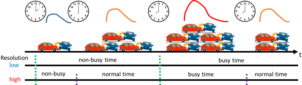
Figure 1: The multi-resolution segmentation of triggering effect of vehicle collisions. The low-resolution (2 segments) and high-resolution (4 segments) partitions provide a hierarchical insight into the dynamic time-varying characteristics.

It is straightforward to see that the conditional intensity of Hawkes process is unchanged over timeshifting because $\mu$ is a constant and $\phi(\cdot)$ only depends on $\tau=t-t_{i}$ not on $t$, which means stationarity. The assumption of stationarity leads to reduced model complexity and easy inference. However, the point process data generated in many real applications has nonstationary properties, which means its first, second and higher order cumulants (moments) are changing over time. Applying the vanilla Hawkes process directly to the nonstationary data is apparently inappropriate. On the other hand, the nonstationarity itself can be an important feature in some applications. For example, in transportation, the influence of a car accident to the road condition is changing between day and night and between busy and non-busy hours (see Fig. 1).

One of the common methods of analyzing nonstationary time series is to use segmentation. This kind of problem is also called change-point problem which is studied in mathematics Carlstein et al. (1994). Given a nonstationary point process data, the segmentation algorithm will divide the whole observation period into several non-overlapping contiguous segments in such a way that each segment is more approximately stationary than the original data and can be assumed to be stationary.

To the best of our knowledge, no segmentation algorithm has been proposed for nonstationary Hawkes process. In this paper, we propose the first multi-resolution segmentation (MRS) algorithm for the nonstationary Hawkes process which can reveal the optimal partition structure in a hierarchical manner. The multi-resolution segmentation is meaningful in real data applications. For example, when the traffic data is analyzed (see Fig. 1), the low-resolution partition (e.g. two segments) corresponds to a “coarser” distinction (e.g. day and night), while the high-resolution partition (e.g. four or six segments) corresponds to a “finer” distinction (e.g. the alternating busy and non-busy hours). This will help us obtain a hierarchical insight into the nonstationary structure of point process data.

As shown later, the performance of the MRS algorithm depends on the choice of hyperparameters. To ease the choice of one hyperparameter, we propose a revised Gaussian process based version which is more robust. Overall, our work makes the following contributions:

• We propose the first multi-resolution segmentation algorithm which provides a hierarchical analysis of the dynamic evolution of nonstationary Hawkes process.

• The MRS depends on the cumulants of Hawkes process which is fast to compute. Consequently, the MRS (linear computation complexity) is faster than the case of direct estimation of baseline intensity and triggering kernel.

• A more robust revised version of MRS is also proposed to ease the choice of one hyperparameter, which is slower but still acceptable in real applications.

2 Related Works

2.1 Nonstationary Hawkes Process

The relaxation of vanilla Hawkes process to nonstationary version mainly consists of two cases: the first case is the extension of baseline intensity $\mu$ to time-changing $\mu(t)$ and the second case is the extension of triggering kernel $\phi(\tau)$ to time-changing $\phi(\tau,t)$. Plenty of state of the arts have performed inference for a time-changing baseline intensity with a stationary triggering kernel Lewis and Mohler (2011); Lemonnier and Vayatis (2014); Tannenbaum and Burak (2017). For both baseline intensity and triggering kernel being nonstationary, Roueff et al. (2016) and Roueff and Von Sachs (2017) provided a general nonparametric estimation theory for the first and second order cumulants of a locally stationary Hawkes process. This method is general but low in computation efficiency: because every point on the two dimensional covariance function $Cov(\tau,t)$ has to be estimated, it is not applicable to real applications. In this sense, the MRS algorithm can be considered as a “coarser” version of Roueff et al. (2016): it combines adjacent small sectors with similar statistical properties into a larger segment and only outputs more heterogeneous segments. Although it is “coarser”, the computation complexity is drastically reduced to make it practical.

2.2 Segmentation of Time Series

Segmentation is a standard method of data analysis to divide a nonstationary time series into a certain number of non-overlapping contiguous homogeneous segments. A heuristic segmentation algorithm is desinged to study the distribution of periods with constant heart rate in Bernaola-Galván et al. (2001). The same method is also applied to analyze changes of the climate Feng et al. (2005). A generalized version is proposed in Bernaola-Galván et al. (2012) to overcome the oversegmentation problem caused by heterogeneities induced by correlations. Similarly, Toth et al. (2010) generalizes this existing algorithm for segmenting regime switching processes. All segmentation methods mentioned above cannot be applied directly to Hawkes process, because they only consider the case of (marked) Poisson process.

3 Cumulants of Hawkes Process

The cumulants of Hawkes process Bacry and Muzy (2016); Jovanović et al. (2015) are used in the MRS algorithm. We consider a 1-variate Hawkes process $\mathbb{N}_{t}$ whose jumps are all of size 1 and whose intensity at time $t$ is $\lambda(t)$. If $\{t_{i}\}$ denotes the jump times of $\mathbb{N}_{t}$, the $\lambda(t)$ can be expressed as (1). If $\mathbb{N}_{t}$ is stationary, the first order cumulant (mean event rate) is

$$\Lambda dt=\mathbb{E}(d\mathbb{N}_{t})=\frac{\mu}{1-\int\phi(\tau)d\tau}dt.$$ (2)

The second order cumulant is

$$Cov(d\mathbb{N}_{t_{1}},d\mathbb{N}_{t_{2}})=\mathbb{E}(d\mathbb{N}_{t_{1}}d\mathbb{N}_{t_{2}})-\mathbb{E}(d\mathbb{N}_{t_{1}})\mathbb{E}(d\mathbb{N}_{t_{2}}).$$ (3)

Because $\mathbb{N}_{t}$ is stationary, $Cov(d\mathbb{N}_{t_{1}},d\mathbb{N}_{t_{2}})$ only depends on $\tau=t_{2}-t_{1}$ and can be expressed as:

$$v(\tau)d\tau=\mathbb{E}(d\mathbb{N}_{0}d\mathbb{N}_{\tau})-\mathbb{E}(d\mathbb{N}_{0})\mathbb{E}(d\mathbb{N}_{\tau}).$$ (4)

Or, it can be rewritten in terms of conditional expectations

$$g(\tau)d\tau=v(\tau)d\tau/\Lambda=\mathbb{E}(d\mathbb{N}_{\tau}|d\mathbb{N}_{0}=1)-\Lambda d\tau.$$ (5)

The $g(\tau)$ will be used throughout this paper.

A stationary Hawkes process is uniquely defined by its first and second order cumulants and there is a bijection between its second order statistics $g(\tau)$ and the triggering kernel $\phi(\tau)$.

4 Multi-resolution Segmentation

We assume there is a set of observation $\{t_{i}\}_{i=1}^{N}$ on $[0,T]$ from a nonstationary Hawkes process where the baseline intensity $\mu$ is piecewise constant and the triggering kernel $\phi(\tau)$ is changing over time $t$. Given $M$, the fundamental idea of MRS is to uniformly divide the observation period $[0,T]$ into $M$ sectors (the highest resolution), e.g. $s_{1},s_{2},...,s_{M}$, where $\{s_{j}\}_{j=1}^{M}$ are sectors and $|s_{j}|$ is the width of the sector. In each $s_{j}$, the point process is assumed to be stationary.

Intuitively, we can estimate the triggering kernel $\phi(\tau)$ in each sector, compare them by adjacent pairs, and find out the most possible partition positions. However, the estimation of $\phi(\tau)$ is time consuming no matter in parametric way (maximum likelihood) or nonparametric way (EM algorithm Lewis and Mohler (2011), Wiener-Hopf equation Bacry and Muzy (2016)), let alone running on all sectors. In order to increase computation efficiency, we do not estimate $\phi(\tau)$ in each sector directly but use the second order statistics $g_{j}(\tau)$ instead which can be estimated faster. The second order statistics $g_{j}(\tau)$ in each sector can be empirically estimated using the empirical version of (5).

The reason we can replace $\phi(\tau)$ in each sector with $g_{j}(\tau)$ is that there is a bijection between them, so the difference between two adjacent $g_{j}(\tau)$ stands for the nonstationarity of $\phi(\tau)$. The difference of two adjacent $g_{j}(\tau)$ is written as a normalized mean squared error (NMSE)

$$NMSE=\mathbb{E}_{\tau}\left((\frac{g_{j}(\tau)}{\int{g_{j}(\tau)}d\tau}-\frac{g_{j+1}(\tau)}{\int{g_{j+1}(\tau)}d\tau})^{2}\right).$$ (6)

In most cases, $g_{j}(\tau)$ is an even function for 1-variate Hawkes process when $\tau\to\pm\infty$, $g_{j}(\tau)\to 0$. If $g_{j}(\tau)$ is expressed as a histogram function $g_{j}(\tau)=\sum_{k=1}^{K}(g_{j}^{k}\delta_{kh})$ where $\delta_{kh}(\tau)=1$ if $(k-1)h\leq\tau<kh$ and $0$ otherwise, $h$ is the bin-width and $g_{j}(\tau)$ is $0$ beyond the support of $Kh$, we can write $g_{j}(\tau)$ as a vector $\mathbf{g}_{j}=[g_{j}^{k}]_{k=1}^{K}$. Equation (6) can be converted to a discrete version

$$NMSE=\frac{\sum_{k=1}^{K}\left((\frac{g_{j}^{k}}{2h\sum_{k=1}^{K}g_{j}^{k}}-\frac{g_{j+1}^{k}}{2h\sum_{k=1}^{K}g_{j+1}^{k}})^{2}\right)}{K}.$$ (7)

Given the NMSE on all candidate cutting positions, if a desired number of segments (the desired output resolution) $R$ is set, we can pick out the largest $R-1$ cutting positions which is the segmentation. The scheme of MRS is shown in Fig. 2. By multi-resolution, we mean by increasing (decreasing) the desired output resolution $R$ the segmentation algorithm will output segments at different resolutions in a hierarchical manner. For example, when $R=M$, the partitioner will output the highest resolution (cutting at all candidate positions), as $R$ becomes smaller the output resolution will be lower (fewer segments will be given out) until there is no cutting at all.

After segmentation, we can piecewisely learn the baseline intensity and triggering kernel on each segment. Specifically, a nonparametric estimation method: Wiener-Hopf equation method Bacry and Muzy (2016) is used. As proved in that work, $\phi(\tau)$ and $g(\tau)$ satisfy the Wiener-Hopf equation

$$g(\tau)=\phi(\tau)+\phi(\tau)*g(\tau),\forall{\tau>0},$$ (8)

where $*$ stands for convolution. In most cases, the Winer-Hopf equation cannot be solved analytically, but there is a lot of literature Noble and Weiss (1959); Atkinson (1976) on how to solve it numerically. A common method is the Nystrom method Nyström (1930). After the solution of $\phi(\tau)$, $\mu$ can be estimated by the first order cumulant (2).

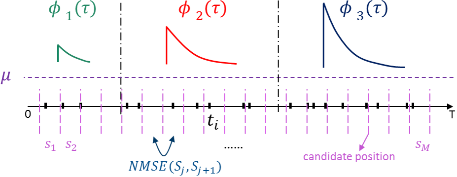
Figure 2: The scheme of multi-resolution segmentation, for simplicity $\mu$ is assumed to be constant and there are 3 different $\phi(\tau)$’s distributed on $[0,T]$.

5 Synthetic Data Experiment

We use thinning algorithm Ogata (1998) to independently generate 40 sets of observations $\{\{t_{i}\}_{i=1}^{N_{l}}\}_{l=1}^{40}$ ($N_{l}$ is the number of points on $l$-th observation) on $[0,1000]$ from a nonstationary Hawkes process where $\mu$’s are $2$, $1.5$, $1$ and triggering kernels are $\phi_{1}(\tau)=1\cdot\exp(-2\tau)$, $\phi_{2}(\tau)=2\cdot\exp(-4\tau)$ and $\phi_{3}(\tau)=3\cdot\exp(-4\tau)$ distributed on $[0,200]$, $[200,600]$ and $[600,1000]$, respectively (see Fig. 2). The goal is to find the underlying partition structure and estimate $\mu$’s and $\phi(\tau)$’s in a nonparametric way. The highest resolution is set to be $M=10$ ($|s_{j}|=100$), $g_{j}(\tau)$ is expressed as a histogram function $g_{j}(\tau)=\sum_{k=1}^{K}(g_{j}^{k}\delta_{kh})$ where $h=0.75$ and $K=8$.

We average the estimated $g_{j}(\tau)$ over 40 sets of independent observations and Tab. 1 shows the multi-resolution segmentation results in a hierarchical manner as $R$ increases from $1$ to the highest resolution $10$. We can see when $R=1$, there is no cutting at all; when $R=3$, the partition positions match with the ground truth; when $R=10$ the algorithm cuts at every candidate position (the highest resolution). To quantify the NMSE caused by estimation variance, the proportion of the minimum threshold corresponding to $R$ over the maximum NMSE is shown in Tab. 1. We can see the NMSE induced by estimation variance is below 11.41% (the last correct cutting is “200” which corresponds to 11.41%), which means the MRS is robust to obtain the correct segmentation.

$R$	1	2	3	4	5
New Position	$\varnothing$	600	200	500	900
$\frac{\text{Min(Threshold)}}{\text{Max(NMSE)}}$	100%	88.45%	11.41%	8.05%	7.15%
$R$	6	7	8	9	10
New Position	400	300	700	800	100
$\frac{\text{Min(Threshold)}}{\text{Max(NMSE)}}$	6.88%	5.17%	2.24%	1.25%	0%

Table 1: Multi-resolution segmentation results. “New Position” is the newly added partition position.

Setting $R=3$, the correct segmentation $[0,200]$, $[200,600]$, $[600,1000]$ is obtained. The next step is to infer $\mu$ and $\phi(\tau)$ on each segment. We empirically estimate the second order statistics $g(\tau)$ on each segment and solve the Winer-Hopf equation (8). The estimated $\hat{\mu}_{1}=2.05$, $\hat{\mu}_{2}=1.64$, $\hat{\mu}_{3}=1.01$ and $\hat{\phi}(\tau)$’s are shown in Fig. 3. We can see the estimation matches with the ground truth.

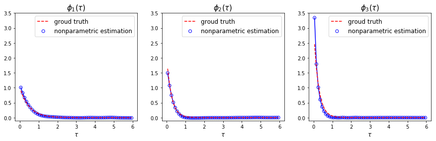
Figure 3: The estimated $\hat{\phi}_{1}(\tau)$, $\hat{\phi}_{2}(\tau)$ and $\hat{\phi}_{3}(\tau)$. The ground truths are $1\cdot\exp(-2\tau)$, $2\cdot\exp(-4\tau)$ and $3\cdot\exp(-4\tau)$, respectively.

5.1 Computation Complexity

In this section, we analyze the computation complexity of MRS algorithm. The MRS algorithm has a linear computation complexity which means it is practical. The complexity of MRS mainly depends on two parameters: the highest resolution $M$ and the size of the observation multiplying the number of bins on $g_{j}(\tau)$: $\mathcal{N}K$ where $\mathcal{N}=\sum_{l}N_{l}$.

The complexity of estimation of $g_{j}(\tau)$ on each sector is $\mathcal{O}(n_{j}K)$ where $n_{j}$ is the number of points in $s_{j}$, consequently, the complexity of all $g_{j}(\tau)$ on all independent observations is $\mathcal{O}(\mathcal{N}K)$. The complexity of NMSE between two adjacent $g_{j}(\tau)$ over $M$ sectors is $\mathcal{O}(M)$. Therefore, the final complexity of MRS is $\mathcal{O}(\mathcal{N}K+M)$. The time consuming experimental results over $\mathcal{N}K$ ($M$) given $M$ ($\mathcal{N}K$) are shown in Fig. 4 which proves the linear conclusion. The consuming time of estimation of $\phi(\tau)$ and $g(\tau)$ is also compared: given 1,896 observation points, the consuming time of $g(\tau)$ is 0.5 second but 38.4 seconds for $\phi(\tau)$, which proves replacing $\phi(\tau)$ with $g(\tau)$ is more efficient.

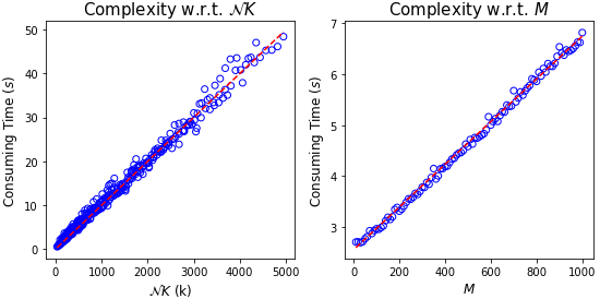
Figure 4: The consuming time of MRS (left: w.r.t. $\mathcal{N}K$ given $M=10$; right: w.r.t. $M$ given $\mathcal{N}K=31,547\times 8$).

5.2 Influence of Hyperparameters

The difference between two adjacent estimated $g_{j}(\tau)$ and $g_{j+1}(\tau)$ is from two sources: the first source is the difference between $\mathbb{E}(g_{j}(\tau))$ and $\mathbb{E}(g_{j+1}(\tau))$ which is the nonstationarity, the second source is the estimation variance of $g_{j}(\tau)$ induced by the choice of hyperparameters. There are two hyperparameters affecting the performance of MRS: $M$ and $K$.

5.2.1 Hyperparameter $M$

Intuitively, the highest resolution $M$ should not be too small or too large. If too small, there are few sectors as the candidate partition positions, consequently, the segmentation result from MRS degrades. If too large, there will be fewer points in each sector $s_{j}$, which means the estimation variance of $g_{j}(\tau)$ is large, consequently, the segmentation result also degrades.

Given $K=8$, the experiment is performed with $M$ from 3 to 20. The segmentation and NMSE results with $R=3$ are shown in Tab. 2 and Fig. 5. We can see when $M$ is in $[10,16]$, the segmentation from MRS is close to the ground truth; when $M>20$, the estimation variance is overwhelming, consequently, the partition positions are misidentified.

$M$	3	10	16	20
Partition Positions	333.3,666.6	200,600	187.5,687.5	150,350
$K$	10	20	30	40
Partition Positions	200,600	200,600	100,200	100,200

Table 2: Segmentation results of MRS w.r.t. $M$ and $K$

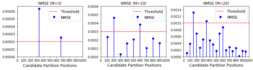
Figure 5: Given $K=8$, the NMSE of MRS w.r.t. $M$. The threshold corresponds to $R=3$ (Only $M=3,10,20$ are shown).

5.2.2 Hyperparameter $K$

Given an appropriate highest resolution $M$, the performance of MRS is also affected by the hyperparameter $K$. The reason behind this phenomenon is that as $K$ becomes larger, there are more bins on $g_{j}(\tau)$ and the estimated $\mathbf{g}_{j}=[g_{j}^{k}]_{k=1}^{K}$ will be overfitting. To show this problem, we perform experiments given the highest resolution $M=10$ but with $K=10,40$ and $100$. The estimated $\mathbf{g}_{1}$ when $K=10,40$ and $100$ is shown in Fig. 7 (only the positive half is shown because of even function). It is clear that the $\mathbf{g}_{1}$ with $K=100$ is overfitting since there are many spikes up and down.

The more bins we have, the larger the estimation variance of $g_{j}(\tau)$ will be, which will lead to a misidentified segmentation. To prove it, the segmentation and NMSE results when $K=10,20,30$ and $40$ with $R=3$ are shown in Tab. 2 and Fig. 6. We can see when $K\geq 30$, the segmentation obtained from MRS does not match with the ground truth any more.

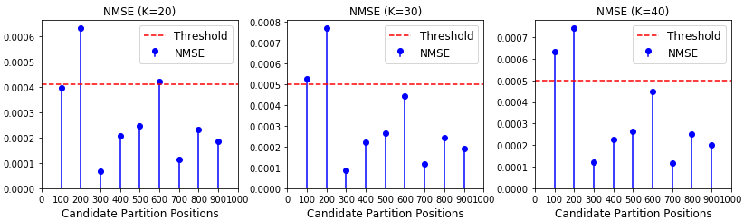
Figure 6: Given $M=10$, the NMSE of MRS w.r.t. $K$. The threshold corresponds to $R=3$ (Only $K=20,30,40$ are shown).

6 Choice of Hyperparameters

Intuitively, a model selection experiment can be performed to obtain the optimal hyperparameters $M$ and $K$. Nevertheless, for a more robust model, we propose a refined MRS algorithm: GP-MRS in this section, by using which we do not need to choose the optimal value of $K$. We can arbitrarily set a large $K$ as GP-MRS can prevent it from overfitting.

6.1 Description of GP-MRS

The key idea of GP-MRS is to use a standard GP regression to smooth the vector $\mathbf{g}_{j}=[g_{j}^{k}]_{k=1}^{K}$ in each sector. Given $\mathbf{g}_{j}=[g_{j}^{1},g_{j}^{2},\dots,g_{j}^{K}]$ in $s_{j}$, the GP regression is performed to evaluate the posterior mean function $\overline{g}_{j}(\tau|g_{j}^{1},g_{j}^{2},\dots,g_{j}^{K})$

$$\overline{g}_{j}(\tau)=\mathbf{d}^{T}\mathbf{C}_{K}^{-1}\mathbf{g}_{j}^{T},$$ (9)

where $\mathbf{C}_{K}$ is the matrix of $C(\tau_{k},\tau_{k^{\prime}})=ker(\tau_{k},\tau_{k^{\prime}})+\sigma^{2}\delta_{kk^{\prime}}$, $\{\tau_{k(k^{\prime})}\}_{k(k^{\prime})=1}^{K}$ are x-values of $K$ training points and $\sigma^{2}$ is the noise variance of training points, $\mathbf{d}=[ker(\tau_{1},\tau),\dots,ker(\tau_{K},\tau)]^{T}$, $\mathbf{g}_{j}$ are y-values of $K$ training points. Here the covariance kernel is squared exponential kernel $ker(x,x^{\prime})=\theta_{0}\exp\left(-\frac{\theta_{1}}{2}\|x-x^{\prime}\|^{2}\right)$ where $\theta_{0}$ and $\theta_{1}$ are hyperparameters of GP. We use $\overline{g}_{j}(\tau)$ to replace the directly estimated $\mathbf{g}_{j}$ in NMSE (7). By using GP-MRS, the NMSE induced by overfitting of $g_{j}(\tau)$ can be effectively eliminated when $K$ is large (comparison between Fig. 6 and Fig. 8).

It is worth noting that GP-MRS cannot be applied to address the problem of $M$ because a too large $M$ will lead to a sparse sector where the GP regression cannot provide a true posterior mean function. To obtain the optimal hyperparameter $M$, an empirical formula is provided: $M\approx\mathcal{N}/250L$ where $L$ is the number of independent observations.

6.2 Synthetic Data Experiment of GP-MRS

We apply the GP-MRS algorithm to the same experiment as in the section 5.2.2. The GP hyperparameters are set to $\theta_{0}=1,\theta_{1}=1,\sigma^{2}=0.01$. It is out of the scope of this paper to discuss how to choose the GP hyperparameters. The estimated $\overline{g}_{1}(\tau)$ when $K=10,40$ and $100$ is shown in Fig. 7. It is clear that the $\overline{g}_{j}(\tau)$ from GP-MRS is stable whatever $K$ is. We also analyze the segmentation and NMSE results with $R=3$ which are shown in Tab. 3 and Fig. 8; we can see the segmentation and NMSE are both stable whatever $K$ is. Conclusively, the GP-MRS can provide the correct segmentation in cases where the MRS does not work.

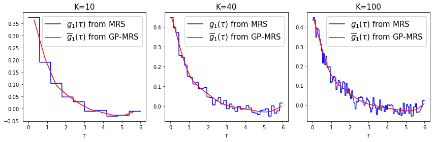
Figure 7: Given $M=10$, the estimated $g_{1}(\tau)$ from MRS and GP-MRS when $K=10,40$ and $100$.

$K$	20	30	40	200
Partition Positions	200,600	200,600	200,600	200,600

Table 3: Segmentation Results of GP-MRS w.r.t. $K$

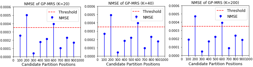
Figure 8: Given $M=10$, the NMSE of GP-MRS w.r.t. $K$. The threshold corresponds to $R=3$ (Only $K=20,40,200$ are shown).The NMSE is nearly unchanged whatever $K$ is.

6.3 Computation Complexity of GP-MRS

For a standard GP, it costs $\mathcal{O}(K^{3})$ for complexity when calculating $K$ training points ($\mathbf{g}_{j}=[g_{j}^{k}]_{k=1}^{K}$). The final complexity of GP-MRS is $\mathcal{O}(\mathcal{N}K+MK^{3})$. Unavoidably, the introduce of GP regression into MRS will make it slower. Given $\mathcal{N}=120,000$ and $M=10$, the consuming time of GP-MRS when $K=40$ is 48.64 seconds on a normal desktop. We can see it is still acceptable when $K$ is not too large.

7 Real Data Experiment

The GP-MRS is applied to a real vehicle collision dataset to discover the hierarchical time-varying characteristics.

7.1 Vehicle Collisions in New York City

The vehicle collision dataset is provided by the New York City Police Department. It contains about 1.05 million vehicle collision records in New York City from July, 2012 to September, 2017. The dataset includes the collision date, time, borough, location, contributing factor and so on.

In daily transportation, the vehicle collision occurring in the past will increase the intensity of vehicle collision occurring in the future because of the traffic jam caused by the initial collision, so there exists a triggering effect from the past collision to the future one. There are already some works trying to model the triggering effect using classic Hawkes process (parametric or nonparametric), but they all assume the stationarity is satisfied. However, this is not the case in real life. As shown later, we reveal the hierarchical time-varying characteristics of triggering kernel and baseline intensity of vehicle collision over 24 hours by using GP-MRS algorithm.

7.1.1 Weekdays

We filter out the collision records on all weekdays from May 1st 2017 to June 30th 2017. There are some collisions occurring at the same time as the data resolution is at minute level, which violates the definition of the temporal point process. To avoid this, we add a small time interval to all the simultaneous records to separate them.

The observation every day is assumed to be independent, so there are 45 sets of independent observations. Totally, 137,578 points are observed. We use the GP-MRS for segmentation which is still fast enough in this case. The whole observation period $T$ is set to 1440 minutes (24 hours a day). The support of $\phi(\tau)$ is set to 8 minutes. The hyperparameters of GP-MRS $\theta_{0}$, $\theta_{1}$, $\sigma^{2}$ are set to 1, 1, 0.01; $K$ is arbitrarily set to 20 and $M$ is set to 12 by using the empirical formula which means the sector size is 120 minutes (2 hours).

When the desired output resolution $R=2$, the consuming time of GP-MRS is about 10 seconds and the cutting positions are 2:00 and 8:00. The segmentation is shown in Fig. 9 left and can be understood as the busy time and non-busy time. After segmentation, we estimate $\mu$ and $\phi(\tau)$ on each segment. The estimated $\mu$’s are $\mu_{1}=0.317$ and $\mu_{2}=0.127$, the estimated $\phi(\tau)$’s are shown in Fig. 10 left. We can see both $\mu_{1}$ and $\phi_{1}(\tau)$ are larger than $\mu_{2}$ and $\phi_{2}(\tau)$ which is consistent with our common sense because the traffic is more crowd in busy time. Additionally, the nonparametricly estimated triggering kernel is not strictly monotonic decreasing: there is a small bump around 5 minutes after the initial collision, which proves the superior flexibility of nonparametric estimation.

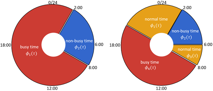
Figure 9: Weekdays: The 24-hour segmentation result of vehicle collisions, 2 segments (left) and 4 segments (right).

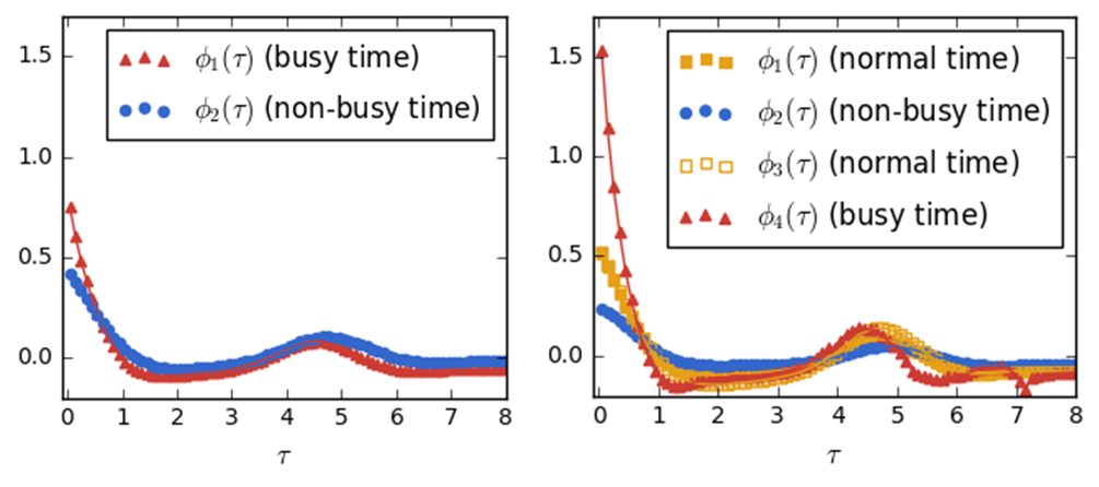
Figure 10: Weekdays: The estimated $\phi(\tau)$ of vehicle collisions, 2 segments (left) and 4 segments (right).

To show the hierarchical multi-resolution property of GP-MRS, the desired output resolution $R$ is increased to 4 and we obtain a finer segmentation. The consuming time in this case is also about 10 seconds and the cutting positions are 2:00, 6:00, 8:00 and 20:00. The segmentation is shown in Fig. 9 right. The segmentation can be understood as the normal time, busy time and non-busy time. The late night is between 2:00 and 6:00 which are non-busy hours; the after-work entertainment hours (from 20:00 to 2:00) together with morning commute hours (from 6:00 to 8:00) are the normal time; the daytime (from 8:00 to 20:00) is the busy time. The estimated $\mu$’s are $\mu_{1}=0.32$, $\mu_{2}=0.12$, $\mu_{3}=0.29$ and $\mu_{4}=0.59$. The estimated $\phi(\tau)$’s are shown in Fig. 10 right. Two normal-time $\phi(\tau)$’s are almost overlapping; both the baseline intensity and triggering kernel of busy time are larger than normal time, larger than non-busy time at the initial stage.

7.1.2 Weekends

We also filter out collision records on all weekends from February 1st 2017 to August 31th 2017. With $R=2$, the cutting positions are 2:00 and 8:00 which are same as weekdays. With $R=3$, we can get a finer segmentation: 2:00, 8:00 and 12:00. The segmentation is shown in Fig. 11. The estimated $\phi(\tau)$’s are shown in Fig. 12.

An interesting phenomenon is that the low-resolution time-varying characteristics of weekdays are similar with that of weekends, but the high-resolution characteristics are very different, e.g. 6:00-8:00 becomes the non-busy time on weekends maybe because of late waking up; 12:00-20:00 becomes the normal time maybe because of less heavy traffic. The multi-resolution segmentation provides a hierarchical insight into the dynamic evolution of vehicle collision.

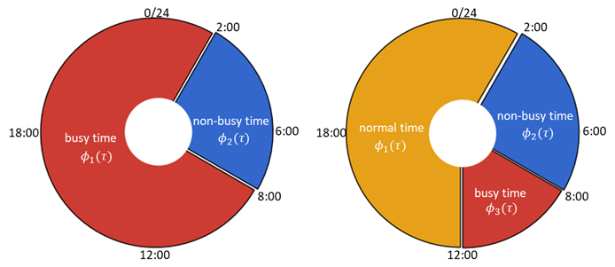
Figure 11: Weekends: The 24-hour segmentation result of vehicle collisions, 2 segments (left) and 3 segments (right).

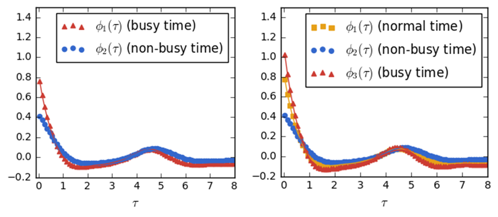
Figure 12: Weekends: The estimated $\phi(\tau)$ of vehicle collisions, 2 segments (left) and 3 segments (right).

7.2 Comparison with Other Models

To show the superiority of our model, we compare the learned results of stationary parametric (vanilla version), stationary nonparametric (nonparametric version) and nonstationary nonparametric Hawkes process (our proposed version).

For stationary parametric version, we assume the triggering kernel is an exponential decay function: $\phi(\tau)=\alpha\cdot\exp(-\beta\tau)$. The inference is performed by maximum likelihood estimation (MLE). The learned $\mu=0.22$ and $\phi(\tau)$ is shown in Fig. 13. For stationary nonparametric version, there is only one triggering kernel which is nonparametric. The inference is performed by Wiener-Hopf equation method. The learned $\mu=0.26$ and $\phi(\tau)$ is shown in Fig.13.

We compare the test error (negative log-likelihood $-logL$) of three models on the vehicle collision test data (weekdays). The result is shown in Fig.13 and our proposed model (the nonstationary nonparametric version) fits the data best.

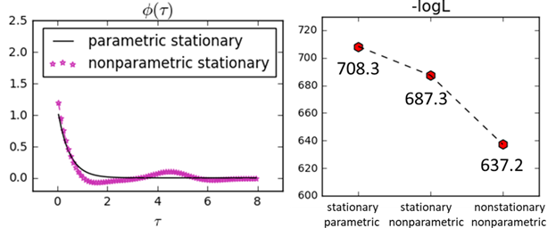
Figure 13: The estimated $\phi(\tau)$ of vehicle collisions of stationary parametric and stationary nonparametric Hawkes process (left). The test error ($-logL$) of three models (right).

8 Conclusions

In this paper, we propose the first MRS algorithm to partition the nonstationary Hawkes process, which provides a hierarchical view of the nonstationary structure. By this way, the hierarchical dynamic time-varying characteristics of nonstaionary Hawkes process can be discovered. Besides, the algorithm is fast because of the use of cumulants. After segmentation, the baseline intensity and triggering kernel are estimated in a nonparametric way. Overall, this is a nonstationary and nonparametric Hawkes process. To ease the choice of hyperparameter $K$, the GP-MRS algorithm is also proposed at the cost of lower efficiency but still acceptable. Both synthetic and real data experiments show the superiority of our proposed model.

References

- Atkinson [1976] Kendall Atkinson. A survey of numerical methods for the solution of Fredholm integral equations of the second kind. 1976.
- Bacry and Muzy [2016] Emmanuel Bacry and Jean-François Muzy. First-and second-order statistics characterization of Hawkes processes and non-parametric estimation. IEEE Transactions on Information Theory, 62(4):2184–2202, 2016.
- Bernaola-Galván et al. [2001] Pedro Bernaola-Galván, Plamen Ch Ivanov, Luís A Nunes Amaral, and H Eugene Stanley. Scale invariance in the nonstationarity of human heart rate. Physical review letters, 87(16):168105, 2001.
- Bernaola-Galván et al. [2012] P Bernaola-Galván, JL Oliver, M Hackenberg, AV Coronado, P Ch Ivanov, and P Carpena. Segmentation of time series with long-range fractal correlations. The European Physical Journal B, 85(6):211, 2012.
- Carlstein et al. [1994] Edward G Carlstein, Hans-Georg Müller, and David Siegmund. Change-point problems. IMS, 1994.
- Du et al. [2016] Nan Du, Hanjun Dai, Rakshit Trivedi, Utkarsh Upadhyay, Manuel Gomez-Rodriguez, and Le Song. Recurrent marked temporal point processes: Embedding event history to vector. In Proceedings of the 22nd ACM SIGKDD International Conference on Knowledge Discovery and Data Mining, pages 1555–1564. ACM, 2016.
- Feng et al. [2005] Guo-Ling Feng, Zhi-Qiang Gong, Wen-Jie Dong, and Jian-Ping Li. Abrupt climate change detection based on heuristic segmentation algorithm. 2005.
- Gupta et al. [2018] Amrita Gupta, Mehrdad Farajtabar, Bistra Dilkina, and Hongyuan Zha. Discrete interventions in Hawkes processes with applications in invasive species management. In IJCAI, pages 3385–3392, 2018.
- Hawkes [1971] Alan G Hawkes. Spectra of some self-exciting and mutually exciting point processes. Biometrika, 58(1):83–90, 1971.
- Jovanović et al. [2015] Stojan Jovanović, John Hertz, and Stefan Rotter. Cumulants of Hawkes point processes. Physical Review E, 91(4):042802, 2015.
- Lemonnier and Vayatis [2014] Remi Lemonnier and Nicolas Vayatis. Nonparametric markovian learning of triggering kernels for mutually exciting and mutually inhibiting multivariate Hawkes processes. In Joint European Conference on Machine Learning and Knowledge Discovery in Databases, pages 161–176. Springer, 2014.
- Lewis and Mohler [2011] Erik Lewis and George Mohler. A nonparametric EM algorithm for multiscale Hawkes processes. Journal of Nonparametric Statistics, 1(1):1–20, 2011.
- Liu et al. [2018] Yanchi Liu, Tan Yan, and Haifeng Chen. Exploiting graph regularized multi-dimensional Hawkes processes for modeling events with spatio-temporal characteristics. In IJCAI, pages 2475–2482, 2018.
- Luo et al. [2015] Dixin Luo, Hongteng Xu, Yi Zhen, Xia Ning, Hongyuan Zha, Xiaokang Yang, and Wenjun Zhang. Multi-task multi-dimensional Hawkes processes for modeling event sequences. In Twenty-Fourth International Joint Conference on Artificial Intelligence, 2015.
- Noble and Weiss [1959] Benjamin Noble and George Weiss. Methods based on the Wiener-Hopf technique for the solution of partial differential equations. Physics Today, 12:50, 1959.
- Nyström [1930] Evert J Nyström. Über die praktische Auflösung von Integralgleichungen mit Anwendungen auf Randwertaufgaben. Acta Mathematica, 54(1):185–204, 1930.
- Ogata [1998] Yosihiko Ogata. Space-time point-process models for earthquake occurrences. Annals of the Institute of Statistical Mathematics, 50(2):379–402, 1998.
- Roueff and Von Sachs [2017] François Roueff and Rainer Von Sachs. Time-frequency analysis of locally stationary Hawkes processes. arXiv preprint arXiv:1704.01437, 2017.
- Roueff et al. [2016] François Roueff, Rainer Von Sachs, and Laure Sansonnet. Locally stationary Hawkes processes. Stochastic Processes and their Applications, 126(6):1710–1743, 2016.
- Tannenbaum and Burak [2017] Neta Ravid Tannenbaum and Yoram Burak. Theory of nonstationary Hawkes processes. Physical Review E, 96(6):062314, 2017.
- Thompson [2012] W Thompson. Point process models with applications to safety and reliability. Springer Science & Business Media, 2012.
- Toth et al. [2010] Bence Toth, Fabrizio Lillo, and J Doyne Farmer. Segmentation algorithm for non-stationary compound Poisson processes. The European Physical Journal B, 78(2):235–243, 2010.
- Weinberg et al. [2007] Jonathan Weinberg, Lawrence D Brown, and Jonathan R Stroud. Bayesian forecasting of an inhomogeneous Poisson process with applications to call center data. Journal of the American Statistical Association, 102(480):1185–1198, 2007.