GCDT: A Global Context Enhanced Deep Transition Architecture
for Sequence Labeling

Abstract

Current state-of-the-art systems for the sequence labeling tasks are typically based on the family of Recurrent Neural Networks (RNNs). However, the shallow connections between consecutive hidden states of RNNs and insufficient modeling of global information restrict the potential performance of those models. In this paper, we try to address these issues, and thus propose a Global Context enhanced Deep Transition architecture for sequence labeling named GCDT. We deepen the state transition path at each position in a sentence, and further assign every token with a global representation learned from the entire sentence. Experiments on two standard sequence labeling tasks show that, given only training data and the ubiquitous word embeddings (Glove), our GCDT achieves 91.96 $F_{1}$ on the CoNLL03 NER task and 95.43 $F_{1}$ on the CoNLL2000 Chunking task, which outperforms the best reported results under the same settings. Furthermore, by leveraging BERT as an additional resource, we establish new state-of-the-art results with 93.47 $F_{1}$ on NER and 97.30 $F_{1}$ on Chunking .

1 Introduction

Sequence labeling tasks, including part-of-speech tagging (POS), syntactic chunking and named entity recognition (NER), are fundamental and challenging problems of Natural Language Processing (NLP). Recently, neural models have become the de-facto standard for high-performance systems. Among various neural networks for sequence labeling, bi-directional RNNs (BiRNNs), especially BiLSTMs Hochreiter and Schmidhuber (1997) have become a dominant method on multiple benchmark datasets Huang et al. (2015); Chiu and Nichols (2016); Lample et al. (2016); Peters et al. (2017).

However, there are several natural limitations of the BiLSTMs architecture. For example, at each time step, the BiLSTMs consume an incoming word and construct a new summary of the past subsequence. This procedure should be highly nonlinear, to allow the hidden states to rapidly adapt to the mutable input while still preserving a useful summary of the past Pascanu et al. (2014). While in BiLSTMs, even stacked BiLSTMs, the transition depth between consecutive hidden states are inherently shallow. Moreover, global contextual information, which has been shown highly useful for model sequence Zhang et al. (2018), is insufficiently captured at each token position in BiLSTMs. Subsequently, inadequate representations flow into the final prediction layer, which leads to the restricted performance of BiLSTMs.

In this paper, we present a global context enhanced deep transition architecture to eliminate the mentioned limitations of BiLSTMs. In particular, we base our network on the deep transition (DT) RNN Pascanu et al. (2014), which increases the transition depth between consecutive hidden states for richer representations. Furthermore, we assign each token an additional representation, which is a summation of hidden states of a specific DT over the whole input sentence, namely global contextual embedding. It’s beneficial to make more accurate predictions since the combinatorial computing between diverse token embeddings and global contextual embedding can capture useful representations in a way that improves the overall system performance.

We evaluate our GCDT on both CoNLL03 and CoNLL2000. Extensive experiments on two benchmarks suggest that, merely given training data and publicly available word embeddings (Glove), our GCDT surpasses previous state-of-the-art systems on both tasks. Furthermore, by exploiting BERT as an extra resource, we report new state-of-the-art $F_{1}$ scores with 93.47 on CoNLL03 and 97.30 on CoNLL2000. The main contributions of this paper can be summarized as follows:

• We are the first to introduce the deep transition architecture for sequence labeling, and further enhance it with the global contextual representation at the sentence level, named GCDT.

• GCDT substantially outperforms previous systems on two major tasks of NER and Chunking. Moreover, by leveraging BERT as an extra resource to enhance GCDT, we report new state-of-the-art results on both tasks.

• We conduct elaborate investigations of global contextual representation, model complexity and effects of various components in GCDT.

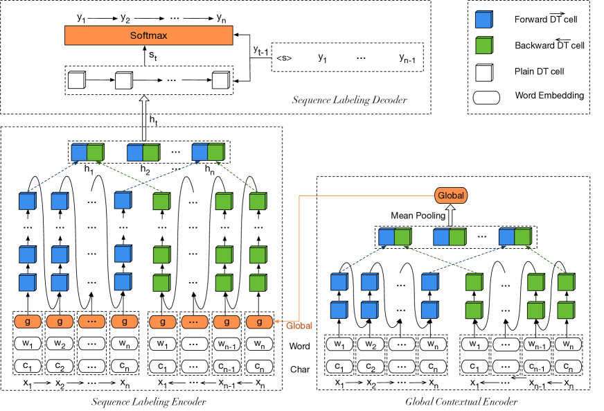
Figure 1: Overview of GCDT. The global contextual encoder (on the right) serves as an enhancement of token representation. The sequence labeling encoder and decoder (on the left) take charge of the task-specific predictions.

2 Background

Given a sequence of $X=\{x_{1},x_{2},\cdots,x_{N}\}$ with $N$ tokens and its corresponding linguistic labels $Y=\{y_{1},y_{2},\cdots,y_{N}\}$ with the equal length, the sequence labeling tasks aim to learn a parameterized mapping function $f_{\theta}:X\rightarrow Y$ from input tokens to task-specific labels.

Typically, the input sentence is firstly encoded into a sequence of distributed representations $\mathbf{X}=\{\mathbf{x}_{1},\mathbf{x}_{2},\cdots,\mathbf{x}_{N}\}$ by character-aware and pre-trained word embeddings. The majority of high-performance models use bidirectional RNNs, BiLSTMs in particular, to encode the token embeddings $\mathbf{X}$ into context-sensitive representations for the final prediction.

Additionally, it’s beneficial to model and predict labels jointly, thus a subsequent conditional random field (CRF Lafferty et al., 2001) is commonly utilized as a decoder layer. At the training stage, those models maximize the log probability of the correct sequence of tags as follows:

$$\log(p(\mathbf{y}|\mathbf{X}))=s(\mathbf{X},\mathbf{y})-\log(\sum_{\widetilde{\mathbf{y}}\in\mathbf{Y}_{x}}e^{s(\mathbf{X},\widetilde{\mathbf{y}})})$$ (1)

where $s(\cdot)$ is the score function and $\mathbf{Y}_{x}$ is the set of all possible sequence of tags. Typically, the Viterbi algorithm Forney (1973) is utilized to search the label sequences with maximum score when decoding:

$$y^{*}=\mathop{\arg\max}_{\widetilde{y}\in Y_{x}}s(x,\widetilde{y})$$ (2)

3 GCDT

3.1 Overview

In this section, we start with a brief overview of our presented GCDT and then proceed to structure the following sections with more details about each submodule. As shown in Figure 1, there are three deep transition modules in our model, namely global contextual encoder, sequence labeling encoder and decoder accordingly.

Token Representation

Given a sentence $X=\{x_{1},x_{2},...,X_{N}\}$ with $N$ tokens, our model first captures each token representation $\mathbf{x}_{t}$ by concatenating three primary embeddings:

$$\mathbf{x}_{t}=[\mathbf{c}_{t};\mathbf{w}_{t};\mathbf{g}]$$ (3)

1. Character level word embedding $\mathbf{c}_{t}$ is acquired from Convolutional Neural Network. (CNN) dos Santos and Zadrozny (2014)

2. Pre-trained word embedding $\mathbf{w}_{t}$ is obtained from the lookup table initialized by Glove.

3. Global contextual embedding $\mathbf{g}$ is extracted from bidirectional DT, and more details will be described in the following paragraphs.

The global embedding $\mathbf{g}$ is computed by mean pooling over all hidden states $\{\mathbf{h}_{1}^{g},\mathbf{h}_{2}^{g},\cdots,\mathbf{h}_{N}^{g}\}$ of global contextual encoder (right part in Figure 1). For simplicity, we can take “DT” as a reinforced Gated Recurrent Unit (GRU Chung et al., 2014), and more details about DT will be described in the next section. Thus $\mathbf{g}$ is computed as follows:

$$\mathbf{g}=\frac{1}{N}\sum_{t=1}^{n}{\mathbf{h}_{t}^{g}}$$ (4)

$$\mathbf{h}_{t}^{g}=[\overrightarrow{\mathbf{h}}_{t}^{g};\overleftarrow{\mathbf{h}}_{t}^{g}]$$ (5)

$$\overrightarrow{\mathbf{h}}_{t}^{g}=\overrightarrow{\mathbf{DT}}_{g}(\mathbf{c_{t}},\mathbf{w_{t}};\mathbf{\theta}_{\overrightarrow{{DT}}_{g}})$$ (6)

$$\overleftarrow{\mathbf{h}}_{t}^{g}=\overleftarrow{\mathbf{DT}}_{g}(\mathbf{c_{t}},\mathbf{w_{t}};\mathbf{\theta}_{\overleftarrow{{DT}}_{g}})$$ (7)

Sequence Labeling Encoder

Subsequently, the concatenated token embeddings $\mathbf{x}_{t}$ (Eq. 3) is fed into the sequence labeling encoder (bottom left part in Figure 1).

$$\mathbf{h}_{t}=[\overrightarrow{\mathbf{h}_{t}};\overleftarrow{\mathbf{h}_{t}}]$$ (8)

$$\overrightarrow{\mathbf{h}_{t}}=\overrightarrow{\mathbf{DT}}_{en}(\mathbf{x}_{t},\overrightarrow{\mathbf{h}}_{t-1};\mathbf{\theta}_{\overrightarrow{{DT}}_{en}})$$ (9)

$$\overleftarrow{\mathbf{h}_{t}}=\overleftarrow{\mathbf{DT}}_{en}(\mathbf{x}_{t},\overleftarrow{\mathbf{h}}_{t-1};\mathbf{\theta}_{\overleftarrow{{DT}}_{en}})$$ (10)

Sequence Labeling Decoder

Considering the $t$-th word in this sentence, the output of sequence labeling encoder $\mathbf{h_{t}}$ along with the past label embedding $\mathbf{y}_{t-1}$ are fed into the decoder (top left part in Figure 1). Subsequently, the output of decoder $\mathbf{s}_{t}$ is transformed into $\mathbf{l}_{t}$ for the final softmax over the tag vocabulary. Formally, the label of word $\mathbf{x}_{t}$ is predicted as the probabilistic equation (Eq. 13)

$$\mathbf{s}_{t}=\mathbf{DT}_{de}(\mathbf{h}_{t},\mathbf{y}_{t-1};\mathbf{\theta}_{DT_{de}})$$ (11)

$$\mathbf{l}_{t}=\mathbf{s}_{t}\mathbf{W}_{l}+\mathbf{b}_{l}$$ (12)

$$P(y_{t}=j|\mathbf{x})=softmax(\mathbf{l}_{t})[j]$$ (13)

As we can see from the above procedures and Figure 1, our GCDT firstly encodes the global contextual representation along the sequential axis by DT, which is utilized to enrich token representations. At each time step, we encode the past label information jointly using the sequence labeling decoder instead of resorting to CRF. Additionally, we employ beam search algorithm to infer the most probable sequence of labels when testing.

3.2 Deep Transition RNN

Deep transition RNNs extend conventional RNNs by increasing the transition depth of consecutive hidden states. Previous studies have shown the superiority of this architecture on both language modeling Pascanu et al. (2014) and machine translation Barone et al. (2017); Meng and Zhang (2019). Particularly, Meng and Zhang Meng and Zhang (2019) propose to maintain a linear transformation path throughout the deep transition procedure with a linear gate to enhance the transition structure.

Following Meng and Zhang Meng and Zhang (2019), the deep transition block in our hierarchical model is composed of two key components, namely Linear Transformation enhanced GRU (L-GRU) and Transition GRU (T-GRU). At each time step, L-GRU first encodes each token with an additional linear transformation of the input embedding, then the hidden state of L-GRU is passed into a chain of T-GRU connected merely by hidden states. Afterwards, the output “state” of the last T-GRU for the current time step is carried over as “state” input of the first L-GRU for the next time step. Formally, in a unidirectional network with transition number of $L$, the hidden state of the $t$-th token in a sentence is computed as:

$$\mathbf{h}_{i}^{0}=\mathbf{L}\textrm{-}\mathbf{GRU}(\mathbf{x}_{i},\mathbf{h}_{i-1}^{L})$$ (14)

$$\mathbf{h}_{i}^{j}=\mathbf{T}\textrm{-}\mathbf{GRU}^{j}(\mathbf{h}_{i}^{j-1})\ \ \ \ \ \ \ 1\leq j\leq L$$ (15)

Linear Transformation Enhanced GRU

L-GRU extends the conventional GRU by an additional linear transformation of the input token embeddings. At time step $t$, the hidden state of L-GRU is computed as follows:

$$\mathbf{h}_{t}=(1-\mathbf{z}_{t})\odot\mathbf{h}_{t-1}+\mathbf{z}_{t}\odot\widetilde{\mathbf{h}}_{t}\ \ \ \ \ \ \ \ \ \ \ \ \$$ (16)

$$\begin{aligned} \widetilde{\mathbf{h}_{t}}=\tanh(&\mathbf{W}_{xh}\mathbf{x}_{t}+\mathbf{r}_{t}\odot(\mathbf{W}_{hh}\mathbf{h}_{t-1}))\\ &+\mathbf{l}_{t}\odot\mathbf{W}_{x}\mathbf{x}_{t}\end{aligned}$$ (17)

where $\mathbf{W}_{xh}$ and $\mathbf{W}_{hh}$ are parameter matrices, and reset gate $\mathbf{r}_{t}$ and update gate $\mathbf{z}_{t}$ are same as GRU:

$$\mathbf{r}_{t}=\sigma(\mathbf{W}_{xr}x_{t}+\mathbf{W}_{hr}\mathbf{h}_{t-1})$$ (18)

$$\mathbf{z}_{t}=\sigma(\mathbf{W}_{xz}\mathbf{x}_{t}+\mathbf{W}_{hz}\mathbf{h}_{t-1})$$ (19)

The linear transformation $\mathbf{W}_{x}\mathbf{x}_{t}$ in candidate hidden state $\widetilde{\mathbf{h}}_{t}$ (Eq. 17) is regulated by the linear gate $\mathbf{l}_{t}$, which is computed as follows:

$$\mathbf{l}_{t}=\sigma(\mathbf{W}_{xl}\mathbf{x}_{t}+\mathbf{W}_{hl}\mathbf{h}_{t-1})$$ (20)

Transition GRU

T-GRU is a special case of conventional GRU, which only takes hidden states from the adjacent lower layer as inputs. At time step $t$ at transition depth $l$, the hidden state of T-GRU is computed as follows:

$$\mathbf{h}^{l}_{t}=(1-\mathbf{z}^{l}_{t})\odot\mathbf{h}^{l-1}_{t}+\mathbf{z}^{l}_{t}\odot\widetilde{\mathbf{h}_{t}}^{l}$$ (21)

$$\widetilde{\mathbf{h}_{t}}^{l}=\tanh(\mathbf{r}_{t}^{l}\odot(\mathbf{W}^{l}_{h}\mathbf{h}_{t}^{l-1}))\ \ \ \ \ \ \$$ (22)

Reset gate $r_{t}$ and update gate $z_{t}$ also only take hidden states as input, which are computed as:

$$\mathbf{r}^{l}=\sigma(\mathbf{W}^{l}_{r}\mathbf{h}^{l-1})$$ (23)

$$\mathbf{z}^{t}=\sigma(\mathbf{W}^{l}_{z}\mathbf{h}^{l-1})$$ (24)

As indicated above, at each time step of our deep transition block, there is a L-GRU in the bottom and several T-GRUs on the top of L-GRU.

3.3 Local Word Representation

Charater-aware word embeddings

It has been demonstrated that character level information (such as capitalization, prefix and suffix) Collobert et al. (2011); dos Santos and Zadrozny (2014) is crucial for sequence labeling tasks. In our GCDT, the character sets consist of all unique characters in datasets besides the special symbol “PAD” and “UNK”. We use one layer of CNN followed by max pooling to generate character-aware word embeddings.

Pre-trained word embeddings

The pre-trained word embeddings have been indicated as a standard component of neural network architectures for various NLP tasks. Since the capitalization feature of words is crucial for sequence labeling tasks Collobert et al. (2011), we adopt word embeddings trained in the case sensitive schema.

Both the character-aware and pre-trained word embeddings are context-insensitive, which are called local word representations compared with global contextual embedding in the next section.

3.4 Global Contextual Embedding

We adopt an independent deep transition RNN named global contextual encoder (right part in Figure 1) to capture global features. In particular, we transform the hidden states of global contextual encoder into a fixed-size vector with various strategies, such as mean pooling, max pooling and self-attention mechanism Vaswani et al. (2017). According to the preliminary experiments, we choose mean pooling strategy considering the balance between effect and efficiency.

In conventional BiRNNs, the global contextual feature is insufficiently modeled at each position, as the nature of recurrent architecture makes RNN partial to the most recent input token. While our context-aware representation is incorporated with local word embeddings directly, which assists in capturing useful representations through combinatorial computing between diverse local word embeddings and the global contextual embedding. We further investigate the effects on positions where the global embedding is used. (Section 5.1)

4 Experiments

4.1 Datasets and Metric

NER

The CoNLL03 NER task Sang and De Meulder (2003) is tagged with four linguistic entity types (PER, LOC, ORG, MISC). Standard data includes train, development and test sets.

Chunking

The CoNLL2000 Chunking task Sang and Buchholz (2000) defines 11 syntactic chunk types (NP, VP, PP, etc.). Standard data includes train and test sets.

Metric

We adopt the BIOES tagging scheme for both tasks instead of the standard BIO2, since previous studies have highlighted meaningful improvements with this scheme Ratinov and Roth (2009). We take the official conlleval as the token-level $F_{1}$ metric. Since the data size if relatively small, we train each final model for 5 times with different parameter initialization and report the mean and standard deviation $F_{1}$ value.

4.2 Implementation Details

All trainable parameters in our model are initialized by the method described by Glorot and Bengio Glorot and Bengio (2010). We apply dropout Srivastava et al. (2014) to embeddings and hidden states with a rate of 0.5 and 0.3 respectively. All models are optimized by the Adam optimizer Kingma and Ba (2014) with gradient clipping of 5 Pascanu et al. (2013). The initial learning rate $\alpha$ is set to 0.008, and decrease with the growth of training steps. We monitor the training process on the development set and report the final result on the test set. One layer CNN with a filter of size 3 is utilized to generate 128-dimension word embeddings by max pooling. The cased, 300d Glove is adapted to initialize word embeddings, which is frozen in all models. In the auxiliary experiments, the output hidden states of BERT are taken as additional word embeddings and kept fixed all the time.

Empirically, We assign the following hyper-parameters with default values except mentioned later. We set batch size to 4096 at the token level, transition number to 4, hidden size of sequence labeling encoder and decoder to 256, hidden size of global contextual encoder to 128.

Models	$F_{1}$
Collobert et al. (2011)*	89.59
Huang et al. (2015)*	90.10
Passos et al. (2014)*	90.90
Lample et al. (2016)	90.94
Yang et al. (2016)*	90.94
Luo et al. (2015)*	91.20
Ma and Hovy (2016)	91.21
Yang et al. (2017b)*$\dagger$	91.26
Zhang et al. (2018)	91.57
Yang et al. (2017a)	91.62
Chiu and Nichols (2016)*$\dagger$	91.62 $\pm$ 0.33
Xin et al. (2018)	91.64 $\pm$ 0.17
GCDT	91.96 $\pm$ 0.04
GCDT + $BERT_{LARGE}$	93.47 $\pm$ 0.03

Table 1: $F_{1}$ scores on CoNLL03. $\dagger$ refers to models trained on both training and development set. * refers to adopting external task-specific resources.

Models	$F_{1}$
Collobert et al. (2011)*	94.32
Huang et al. (2015)*	94.46
Yang et al. (2017b)	94.66
Zhai et al. (2017)	94.72
Hashimoto et al. (2017)	95.02
Søgaard and Goldberg (2016)	95.28
Xin et al. (2018)	95.29 $\pm$ 0.08
GCDT	95.43 $\pm$ 0.06
GCDT + $BERT_{LARGE}$	97.30 $\pm$ 0.03

Table 2: $F_{1}$ scores on CoNLL2000 Chunking task. * refers to adopting external task-specific resources (like Gazetteers or annotated data).

4.3 Main Results

The main results of our GCDT on the CoNLL03 and CoNLL2000 are illustrated in Table 1 and Table 2 respectively. Given only standard training data and publicly available word embeddings, our GCDT achieves state-of-the-art results on both tasks. It should be noted that some results on NER are not comparable to ours directly, as their final models are trained on both training and development data . More notably, our GCDT surpasses the models that exploit additional task-specific resources or annotated corpora Luo et al. (2015); Yang et al. (2017b); Chiu and Nichols (2016).

Additionally, we conduct experiments by leveraging the well-known BERT as an external resource for relatively fair comparison with models that utilize external language models trained on massive corpora. Especially, Rei Rei (2017) and Liu et al. Liu et al. (2017) build task-specific language models only on supervised data. Table 3 and Table 4 show that our GCDT outperforms previous state-of-the-art results substantially at 93.47 (+0.38) on NER and 97.30 (+0.30) on Chunking when contrasted with a collection of highly competitive baselines.

Models	$F_{1}$
Rei (2017)	86.26
Liu et al. (2017)	91.71 $\pm$ 0.10
Peters et al. (2017)$\dagger$	91.93 $\pm$ 0.19
Peters et al. (2018)	92.20
Clark et al. (2018)	92.61
Devlin et al. (2018) $BERT_{BASE}$	92.40
Devlin et al. (2018) $BERT_{LARGE}$	92.80
Akbik et al. (2018)$\dagger$	93.09
GCDT + $BERT_{LARGE}$	93.47 $\pm$ 0.03

Table 3: $F_{1}$ scores on the CoNL03 NER task by leveraging language model, $\dagger$ refers to models trained on both training and development data. We establish new state-of-the-art result on this task.

Models	$F_{1}$
Rei (2017)	93.88
Liu et al. (2017)	95.96 $\pm$ 0.08
Peters et al. (2017)	96.37 $\pm$ 0.05
Akbik et al. (2018)	96.72 $\pm$ 0.05
Clark et al. (2018)	97.00
GCDT + $BERT_{LARGE}$	97.30 $\pm$ 0.03

Table 4: $F_{1}$ scores on the CoNLL2000 Chunking task by leveraging language model. We establish new state-of-the-art result on this task.

5 Analysis

We choose the CoNLL03 NER task as example to elucidate the properties of our GCDT and conduct several additional experiments.

5.1 Where to Use the Global Representation?

In this experiment, we investigate the effects of locations on the global contextual embedding in our hierarchical model. In particular, we use the global embedding $\mathbf{g}$ to augment:

• input of final softmax layer ;
  $\mathbf{x}_{k}^{softmax}=[\mathbf{h}_{k}^{decoder};\mathbf{y}_{k-1};\mathbf{g}]$

• input of sequence labeling decoder;
  $\mathbf{x}_{k}^{decoder}=[\mathbf{h}_{k}^{encoder};\mathbf{y}_{k-1};\mathbf{g}]$

• input of sequence labeling encoder;
  $\mathbf{x}_{k}^{encoder}=[\mathbf{w}_{k};\mathbf{c}_{k};\mathbf{g}]$

#	Use global embedding at	$F_{1}$
0	None	91.60
1	Input of final softmax	91.48
2	Input of sequence labeling decoder	91.45
3	Input of sequence labeling encoder	91.96

Table 5: Comparison of CoNLL03 test $F_{1}$ when the global contextual embedding is used at different layers.

Table 5 shows that the global embedding $\mathbf{g}$ improves performance when utilized at the relative low layer (row 3) , while $\mathbf{g}$ may do harm to performances when adapted at the higher layers (row 0 vs. row 1 & 2). In the last option, $\mathbf{g}$ is incorporated to enhance the input token representation for sequence labeling encoder, the combinatorial computing between the multi-granular local word embeddings ($\mathbf{w}_{k}$ and $\mathbf{c}_{k}$) and global embedding $\mathbf{g}$ can capture more specific and richer representations for the prediction of each token, and thus improves overall system performance. While the other two options (row 1, 2) concatenate the highly abstract $\mathbf{g}$ with hidden states ($\mathbf{h}_{k}^{encoder}$ or $\mathbf{h}_{k}^{decoder}$) from the higher layers, which may bring noise to token representation due to the similar feature spaces and thus hurt task-specific predictions.

5.2 Comparing with Stacked RNNs

Although our proposed GCDT bears some resemblance to the conventional stacked RNNs, they are very different from each other. Firstly, although the stacked RNNs can process very deep architectures, the transition depth between consecutive hidden states in the token level is still shallow.

Secondly, in the stacked RNNs, the hidden states along the sequential axis are simply fed into the corresponding positions of the higher layers, namely only position-aware features are transmitted in the deep architecture. While in GCDT, the internal states in all token position of the global contextual encoder are transformed into a fixed-size vector. This contextual-aware representation provides more general and informative features of the entire sentence compared with stacked RNNs.

To obtain rigorous comparisons, we stack two layers of deep transition RNNs instead of conventional RNNs with similar parameter numbers of GCDT. According to the results in Table 6, the stacked-DT improves the performance of the original DT slightly, while there is still a large margin between GCDT and the stacked-DT. As we can see, our GCDT achieves a much better performance than stacked-DT with a smaller parameter size, which further verifies that our GCDT can effectively leverage global information to learn more useful representations for sequence labeling tasks.

Model	# Parameters	$F_{1}$
DT	5.6M	91.60
stacked-DT	8.4M	91.61
GCDT	7.4M	91.96

Table 6: Comparison of CoNLL03 test $F_{1}$ between stacked RNNs and GCDT.

5.3 Ablation Experiments

We conduct ablation experiments to investigate the impacts of various components in GCDT. More specifically, we remove one kind of token embedding from char-aware, pre-trained and global embeddings for sequence labeling encoder each time, and utilize DT or conventional GRU with similar model sizes . Results of different combinations are presented in Table 7.

Given the same input embeddings, DT surpasses the conventional GRU substantially in most cases, which further demonstrates the superiority of DT in sequence labeling tasks. Our observations on character-level and pre-trained word embeddings suggest that they have a significant impact on highly competitive results (row 1 & 3 vs. row 5), which is consistent with previous work dos Santos and Zadrozny (2014); Lample et al. (2016). Furthermore, the global contextual embedding substantially improves the performances on both DT and GRU based models (row 6 & 7 vs. row 4 & 5).

#	Embeddings	RNN	$F_{1}$
0	No char	GRU	91.14
1	No char	DT	90.94
2	No Glove	GRU	87.23
3	No Glove	DT	88.59
4	No global	GRU	91.32
5	No global	DT	91.60
6	All	GRU	91.42
7	All	DT	91.96

Table 7: Ablation experiments on the CoNLL03 to investigate the impacts of various components, where “char” indicates character-aware word embeddings, “Glove” indicates pre-trained word embeddings, and “global” indicates global contextual embedding.

BERT			$F_{1}$
Type	Layer	Pooling
BASE	6	first	92.70
		max	92.88
		mean	92.99
	12	first	92.89
		max	92.74
		mean	92.92
LARGE	12	first	92.88
		max	93.23
		mean	93.36
	18	first	93.18
		max	93.07
		mean	93.47
	24	first	92.57
		max	92.60
		mean	92.83

Table 8: Comparison of CoNLL03 $F_{1}$ scores when various types, layers and pooling strategies of BERT are employed. “first” indicates the first sub-word embedding, “mean” and “max” refer to mean and max pooling correspondingly.

#	Global Contextual Encoder	Sequence Labeling Module	# Parameters	$F_{1}$
0	GRU-384	GRU-384	7.8M	91.42
1	GRU-384	DT4-256	9.5M	91.53
2	GRU-512	DT4-256	11.2M	91.49
3	DT2-128	GRU-384	5.7M	91.45
4	DT2-128	DT4-256	7.2M	91.72
5	DT4-128	DT4-256	7.4M	91.96

Table 9: $F_{1}$ scores on the CoNLL03 and parameter sizes of various models, where “GRU-384” indicates the conventional GRU with hidden size of 384, while “DT2-128” refers to deep transition RNN with transition number of 2 and hidden size of 128, similarly for “DT4-256”.

5.4 Effect of BERT

WordPiece is adopted to tokenize sequence in BERT, which may cut a word into pieces, such as converting “Johanson” into “Johan ##son”. Therefore, additional efforts should be taken to maintain alignments between input tokens and their corresponding labels. Three strategies are conducted to obtain the exclusive BERT embedding of each token in a sequence. Firstly, we take the first sub-word as the whole word embedding after tokenization, which is employed in the original paper of BERT Devlin et al. (2018). Mean and max poolings are used as the latter two strategies. Results of various combinations of BERT type, layer and pooling strategy are illustrated in Table 8.

It’s reasonable that BERT trained on large model surpasses the smaller one in most cases due to the larger model capacity and richer contextual representation. For the pooling strategy, “mean” is considered to capture more comprehensive representations of rare words than “first” and “max”, thus better average performances. Additionally, we hypothesize that the higher layers in BERT encode more abstract and semantic features, while the lower ones prefer general and syntax information, which is more helpful for our NER and Chunking tasks. These hypotheses are consistent with results emerged in Table 8.

5.5 Model Complexity

One way of measuring the complexity of a neural model is through the total number of trainable parameters. In GCDT, the global contextual encoder increases parameter numbers of the sequence labeling encoder due to the enlargement of input dimensions, thus we run additional experiments to verify whether the increment of parameters has a great affection on performances. Empirically, we replace DT with conventional GRU in the global contextual encoder and sequence labeling module (both encoder and decoder) respectively. Results of various combinations are shown in Table 9.

Observations on parameter numbers show that DT outperforms GRU substantially, with a smaller size (row 4 & 5 vs. row 0). From the perspective of global contextual encoder, DT gives slightly better result compared with GRU (row 3 vs. row 0). We observe similar results in the sequence labeling module (row 1 & 2 vs. row 0). Intuitively, it should further improve performance when utilizing DT in both modules, which is consistent with the observations in Table 9 (row 4 & 5 vs. row 0).

6 Related Work

Neural Sequence Labeling

Collobert et al. Collobert et al. (2011) propose a seminal neural architecture for sequence labeling, which learns useful representation from pre-trained word embeddings instead of hand-crafted features. Huang et al. Huang et al. (2015) develop the outstanding BiLSTMs-CRF architecture, which is improved by incorporating character-level LSTM Lample et al. (2016), GRU Yang et al. (2016), CNN dos Santos and Zadrozny (2014); Xin et al. (2018), IntNet Xin et al. (2018). The shallow connections between consecutive hidden states in those models inspire us to deepen the transition path for richer representation.

More recently, there has been a growing body of work exploring to leverage language model trained on massive corpora in both character level Peters et al. (2017, 2018); Akbik et al. (2018) and token level Devlin et al. (2018). Inspired by the effectiveness of language model embeddings, we conduct auxiliary experiments by leveraging the well-known BERT as an additional feature.

Exploit Global Information

Chieu and Ng Chieu and Ng (2002) explore the usage of global feature in the whole document by the co-occurrence of each token, which is fed into a maximum entropy classifier. With the widespread application of distributed word representations Mikolov et al. (2013) and neural networks Collobert et al. (2011); Huang et al. (2015) in sequence labeling tasks, the global information is encoded into hidden states of BiRNNs. Specially, Yang et al. Yang et al. (2017a) leverage global sentence patterns for NER reranking. Inspired by the global sentence-level representation in S-LSTM Zhang et al. (2018), we propose a more concise approach to capture global information, which has been demonstrated more effective on sequence lableing tasks.

Deep Transition RNN

Deep transition recurrent architecture extends conventional RNNs by increasing the transition depth between consecutive hidden states. Previous studies have shown the superiority of this architecture on both language model Pascanu et al. (2014) and machine translation Barone et al. (2017); Meng and Zhang (2019). We follow the deep transition architecture in Meng and Zhang (2019), and extend it into a hierarchical model with the global contextual representation at the sentence level for sequence labeling tasks.

7 Conclusion

We propose a novel hierarchical neural model for sequence labeling tasks (GCDT), which is based on the deep transition architecture and motivated by global contextual representation at the sentence level. Empirical studies on two standard datasets suggest that GCDT outperforms previous state-of-the-art systems substantially on both CoNLL03 NER task and CoNLL2000 Chunking task without additional corpora or task-specific resources. Furthermore, by leveraging BERT as an external resource, we report new state-of-the-art $F_{1}$ scores of 93.47 on CoNLL03 and 97.30 on CoNLL2000.

In the future, we would like to extend GCDT to other analogous sequence labeling tasks and explore its effectiveness on other languages.

References

- Akbik et al. (2018) Alan Akbik, Duncan Blythe, and Roland Vollgraf. 2018. Contextual string embeddings for sequence labeling. In Proceedings of the 27th International Conference on Computational Linguistics, pages 1638–1649. Association for Computational Linguistics.
- Barone et al. (2017) Antonio Valerio Miceli Barone, Jindrich Helcl, Rico Sennrich, Barry Haddow, and Alexandra Birch. 2017. Deep architectures for neural machine translation. CoRR, abs/1707.07631.
- Chieu and Ng (2002) Hai Leong Chieu and Hwee Tou Ng. 2002. Named entity recognition: A maximum entropy approach using global information. In COLING 2002: The 19th International Conference on Computational Linguistics.
- Chiu and Nichols (2016) Jason Chiu and Eric Nichols. 2016. Named entity recognition with bidirectional lstm-cnns. Transactions of the Association for Computational Linguistics, 4:357–370.
- Chung et al. (2014) Junyoung Chung, Çaglar Gülçehre, KyungHyun Cho, and Yoshua Bengio. 2014. Empirical evaluation of gated recurrent neural networks on sequence modeling. CoRR, abs/1412.3555.
- Clark et al. (2018) Kevin Clark, Minh-Thang Luong, Christopher D. Manning, and Quoc Le. 2018. Semi-supervised sequence modeling with cross-view training. In Proceedings of the 2018 Conference on Empirical Methods in Natural Language Processing, pages 1914–1925. Association for Computational Linguistics.
- Collobert et al. (2011) Ronan Collobert, Jason Weston, Léon Bottou, Michael Karlen, Koray Kavukcuoglu, and Pavel Kuksa. 2011. Natural language processing (almost) from scratch. Journal of Machine Learning Research, 12(Aug):2493–2537.
- Devlin et al. (2018) Jacob Devlin, Ming-Wei Chang, Kenton Lee, and Kristina Toutanova. 2018. Bert: Pre-training of deep bidirectional transformers for language understanding. arXiv preprint arXiv:1810.04805.
- Forney (1973) G David Forney. 1973. The viterbi algorithm. Proceedings of the IEEE, 61(3):268–278.
- Glorot and Bengio (2010) Xavier Glorot and Yoshua Bengio. 2010. Understanding the difficulty of training deep feedforward neural networks. In Proceedings of the thirteenth international conference on artificial intelligence and statistics, pages 249–256.
- Hashimoto et al. (2017) Kazuma Hashimoto, caiming xiong, Yoshimasa Tsuruoka, and Richard Socher. 2017. A joint many-task model: Growing a neural network for multiple nlp tasks. In Proceedings of the 2017 Conference on Empirical Methods in Natural Language Processing, pages 1923–1933. Association for Computational Linguistics.
- Hochreiter and Schmidhuber (1997) Sepp Hochreiter and Jürgen Schmidhuber. 1997. Long short-term memory. Neural Computation, 9(8):1735–1780.
- Huang et al. (2015) Zhiheng Huang, Wei Xu, and Kai Yu. 2015. Bidirectional LSTM-CRF models for sequence tagging. CoRR, abs/1508.01991.
- Kingma and Ba (2014) Diederik P Kingma and Jimmy Ba. 2014. Adam: A method for stochastic optimization. arXiv preprint arXiv:1412.6980.
- Lafferty et al. (2001) John Lafferty, Andrew McCallum, and Fernando CN Pereira. 2001. Conditional random fields: Probabilistic models for segmenting and labeling sequence data.
- Lample et al. (2016) Guillaume Lample, Miguel Ballesteros, Sandeep Subramanian, Kazuya Kawakami, and Chris Dyer. 2016. Neural architectures for named entity recognition. In Proceedings of the 2016 Conference of the North American Chapter of the Association for Computational Linguistics: Human Language Technologies, pages 260–270. Association for Computational Linguistics.
- Liu et al. (2017) Liyuan Liu, Jingbo Shang, Frank F. Xu, Xiang Ren, Huan Gui, Jian Peng, and Jiawei Han. 2017. Empower sequence labeling with task-aware neural language model. CoRR, abs/1709.04109.
- Luo et al. (2015) Gang Luo, Xiaojiang Huang, Chin-Yew Lin, and Zaiqing Nie. 2015. Joint entity recognition and disambiguation. In Proceedings of the 2015 Conference on Empirical Methods in Natural Language Processing, pages 879–888.
- Ma and Hovy (2016) Xuezhe Ma and Eduard Hovy. 2016. End-to-end sequence labeling via bi-directional lstm-cnns-crf. In Proceedings of the 54th Annual Meeting of the Association for Computational Linguistics (Volume 1: Long Papers), pages 1064–1074. Association for Computational Linguistics.
- Meng and Zhang (2019) Fandong Meng and Jinchao Zhang. 2019. DTMT: A novel deep transition architecture for neural machine translation. AAAI.
- Mikolov et al. (2013) Tomas Mikolov, Ilya Sutskever, Kai Chen, Greg S Corrado, and Jeff Dean. 2013. Distributed representations of words and phrases and their compositionality. In Advances in neural information processing systems, pages 3111–3119.
- Pascanu et al. (2014) Razvan Pascanu, Caglar Gulcehre, Kyunghyun Cho, and Yoshua Bengio. 2014. How to construct deep recurrent neural networks. In ICLR.
- Pascanu et al. (2013) Razvan Pascanu, Tomas Mikolov, and Yoshua Bengio. 2013. On the difficulty of training recurrent neural networks. In International conference on machine learning, pages 1310–1318.
- Passos et al. (2014) Alexandre Passos, Vineet Kumar, and Andrew McCallum. 2014. Lexicon infused phrase embeddings for named entity resolution. In Proceedings of the Eighteenth Conference on Computational Natural Language Learning, pages 78–86. Association for Computational Linguistics.
- Peters et al. (2017) Matthew Peters, Waleed Ammar, Chandra Bhagavatula, and Russell Power. 2017. Semi-supervised sequence tagging with bidirectional language models. In Proceedings of the 55th Annual Meeting of the Association for Computational Linguistics (Volume 1: Long Papers), pages 1756–1765. Association for Computational Linguistics.
- Peters et al. (2018) Matthew Peters, Mark Neumann, Mohit Iyyer, Matt Gardner, Christopher Clark, Kenton Lee, and Luke Zettlemoyer. 2018. Deep contextualized word representations. In Proceedings of the 2018 Conference of the North American Chapter of the Association for Computational Linguistics: Human Language Technologies, Volume 1 (Long Papers), pages 2227–2237. Association for Computational Linguistics.
- Ratinov and Roth (2009) Lev Ratinov and Dan Roth. 2009. Design challenges and misconceptions in named entity recognition. In Proceedings of the thirteenth conference on computational natural language learning, pages 147–155. Association for Computational Linguistics.
- Rei (2017) Marek Rei. 2017. Semi-supervised multitask learning for sequence labeling. In Proceedings of the 55th Annual Meeting of the Association for Computational Linguistics (Volume 1: Long Papers), pages 2121–2130. Association for Computational Linguistics.
- Sang and Buchholz (2000) Erik F Sang and Sabine Buchholz. 2000. Introduction to the conll-2000 shared task: Chunking. arXiv preprint cs/0009008.
- Sang and De Meulder (2003) Erik F Sang and Fien De Meulder. 2003. Introduction to the conll-2003 shared task: Language-independent named entity recognition. arXiv preprint cs/0306050.
- dos Santos and Zadrozny (2014) Cícero Nogueira dos Santos and Bianca Zadrozny. 2014. Learning character-level representations for part-of-speech tagging. In ICML.