The [C ii] / [N ii] ratio in $3<z<6$ sub-millimetre galaxies from the South Pole Telescope survey

Abstract

We present Atacama Compact Array and Atacama Pathfinder Experiment observations of the [N ii] 205 $\mu$m fine-structure line in 40 sub-millimetre galaxies lying at redshifts $z=3$ to $6$, drawn from the 2500 deg² South Pole Telescope survey. This represents the largest uniformly selected sample of high-redshift [N ii] 205 $\mu$m measurements to date. 29 sources also have [C ii] 158 $\mu$m line observations allowing a characterization of the distribution of the [C ii] to [N ii] luminosity ratio for the first time at high-redshift. The sample exhibits a median L${}_{\textrm{\small\mbox{[C~{}{\sc ii}]}}}$/L${}_{\textrm{\small\mbox{[N~{}{\sc ii}]}}}$ $\approx$ 11.0 and interquartile range of 5.0 to 24.7. These ratios are similar to those observed in local (U)LIRGs, possibly indicating similarities in their interstellar medium. At the extremes, we find individual sub-millimetre galaxies with L${}_{\textrm{\small\mbox{[C~{}{\sc ii}]}}}$/L${}_{\textrm{\small\mbox{[N~{}{\sc ii}]}}}$ low enough to suggest a smaller contribution from neutral gas than ionized gas to the [C ii] flux and high enough to suggest strongly photon or X-ray region dominated flux. These results highlight a large range in this line luminosity ratio for sub-millimetre galaxies, which may be caused by variations in gas density, the relative abundances of carbon and nitrogen, ionization parameter, metallicity, and a variation in the fractional abundance of ionized and neutral interstellar medium.

1 Introduction

Observing far-infrared (FIR) luminous galaxies at high-redshift is a crucial step in understanding the evolution of galaxies as they highlight periods of intense star formation which may represent pivotal growth periods in a galaxy’s evolution (e.g., Casey et al. 2014). At z $\sim$ 2, sub-millimetre galaxies (SMGs) may have accounted for 50% of star formation in the universe (Wardlow et al., 2011). At high-redshift, the FIR emission from these galaxies peaks at sub-millimetre wavelengths in the observer’s frame, allowing effective selection at sub-mm or longer wavelengths. The peak redshift at which they are predominantly found depends on the wavelength of the survey: at $\sim$ 850$\mu$m, the peak is close to $z\sim 2.5$ (Chapman et al., 2003, 2005), while at the 1 to 2 mm regime of the SPT survey, the median redshift increases to $\langle z\rangle\sim 4$ (Weiß et al. 2013, Strandet et al. 2016). Regardless of wavelength of selection, they display rapid star formation sometimes exceeding $10^{3}$ $\mathrm{M}_{\odot}/\mathrm{yr}$ (Swinbank et al., 2014), and have stellar masses on the order of $10^{11}$ $\mathrm{M}_{\odot}$ (Hainline et al., 2011; Michalowski, M. J. et al., 2012; Ma et al., 2015). Their rapid evolution early in cosmic time continues to push current simulations to match their detailed properties (e.g. Shimizu et al. 2012; Hayward et al. 2013; Narayanan et al. 2015; Cowley et al. 2017).

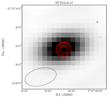
(a)

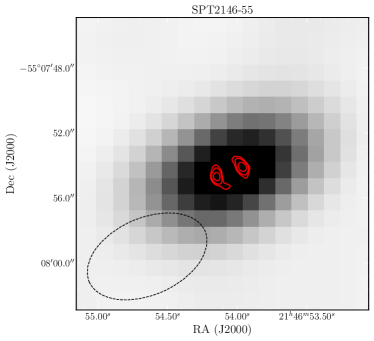
(b)

Figure 1: Two examples of our ALMA ACA [N ii] line observations, one from each of band 6 and 7, showing the [N ii] detection as a channel map optimized over the FWHM of the line in grey-scale. The red contours represent continuum from higher resolution band-7 ALMA imaging, and demonstrate that the ACA beam does not resolve even the largest lensed SMGs in our sample. The beam size is represented in the bottom left corner by the black dashed line ellipse. Top panel: [N ii] observations of SPT0418–47 in band-7. Bottom panel: [N ii] observations of SPT2146–55 in band-6.

In high-redshift dusty galaxies more traditional optical and ultraviolet line diagnostics are not possible due to high dust attenuation. Fine-structure transition lines such as [C ii] 158 $\mu$m (${}^{2}\mathrm{P}_{3/2}\rightarrow{}^{2}\mathrm{P}_{1/2}$) and [N ii] 205 $\mu$m (${}^{3}\mathrm{P}_{1}\rightarrow{}^{3}\mathrm{P}_{0}$) (hereafter [C ii] and [N ii]) offer important insight into the properties of the interstellar medium (ISM) and importantly are not significantly affected by dust attenuation. The [C ii]-to-[N ii] ratio can probe physical parameters of the ISM. Assuming a pressure-equilibrium gas cloud with a range of gas densities and ionization parameters at its illuminated surface, Nagao et al. (2012) used cloudy modelling (Ferland et al., 1998) to show that the [C ii]-to-[N ii] flux ratio decreases monotonically with gas metallicity. However, because of dependencies of this ratio on the unknown density and ionization parameters, additional lines such as [N ii] 122 $\mu$m and [O i] 145 $\mu$m are needed to break the degeneracy with these parameters (Nagao et al., 2012). Since [C ii] emission originates from both ionized and neutral gas, while [N ii] is primarily emitted from ionized gas, the [C ii]-to-[N ii] ratio can probe the abundance of ionized and neutral gas regions in a galaxy’s ISM (Decarli et al., 2014).

Several previous studies have used the [C ii]-to-[N ii] line ratio to investigate the ISM properties of luminous, high-redshift galaxies including SMGs (e.g. Nagao et al. 2012, Decarli et al. 2014, Béthermin et al. 2016, Pavesi et al. 2016, Umehata et al. 2017, Pavesi et al. 2018, Tadaki et al. 2019). They measure a large range in the line ratio, indicating these galaxies have diverse ISM conditions. At low-redshift, Herrera-Camus et al. (2016) used [N ii] 122 $\mu$m and 205 $\mu$m emission lines to constrain gas density and SFR, while Cormier et al. (2015) found (using the [N ii] 122 $\mu$m line) that the ionized medium contributes little to the [C ii] emission in their dwarf galaxy sample.

This paper presents measurements of [N ii] in 40 gravitationally lensed SMGs between $3<z<6$ from the SPT survey. This is the first uniformly selected large sample of SMGs with [N ii] detections at high-redshift. When combined with 29 additional [C ii] observations, these measurements allow us to make the first characterization of the high-redshift L${}_{\textrm{\small\mbox{[C~{}{\sc ii}]}}}$/L${}_{\textrm{\small\mbox{[N~{}{\sc ii}]}}}$ distribution in SMGs using a uniformly selected sample. Its wide redshift range makes it a unique sample to study the possible evolution in the ISM of high-redshift SMGs in comparison to local Luminous Infra-red Galaxies (LIRGs). Since the SPT galaxies are gravitationally lensed, even the relatively faint [N ii] emitting sources can be detected quickly with the Morita Atacama Compact Array (ACA) of the Atacama Large Millimeter/submillimeter Array (ALMA). This allows for a complete characterization of the L${}_{\textrm{\small\mbox{[C~{}{\sc ii}]}}}$/L${}_{\textrm{\small\mbox{[N~{}{\sc ii}]}}}$ ratio in the ultra-luminous galaxy population (L${}_{\textrm{\sc fir}}>10^{12}$ L_⊙) at high-redshift. We assume a Hubble constant $H_{0}=70$ km s^-1 Mpc^-1 and density parameters $\Omega_{\Lambda}=0.7$ and $\Omega_{\rm m}=0.3$ throughout.

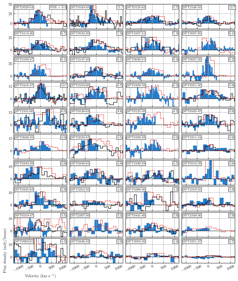
Figure 2: Observed [N ii] 205 $\mu$m (blue background), [C ii] 158 $\mu$m (black line), and CO (dashed red line) line profiles for the 40 ALMA observed sources, excluding SPT2132–58 which was presented in Béthermin et al. (2016). Sources are ordered by observed [N ii] 205 $\mu$m flux, given in Table 1. The [N ii] spectra are single pixel extractions. The signal-to-noise ratio from the optimal integrated line detection is given in the upper-right corner of each panel. The CO line is either CO(4–3) or CO(5–4) depending on source redshift (see Strandet et al. 2016). Both CO and [C ii] lines are normalized to the peak [N ii] flux for each source (see Table 1 for [C ii] flux). The zero velocity is determined according to redshifts presented in Strandet et al. (2016).

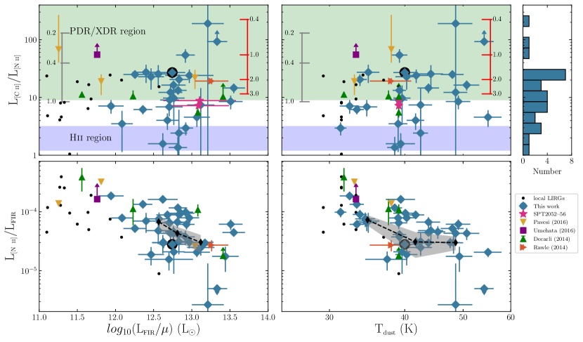
Figure 3: Comparison of key properties of our lensed sample of [N ii] and [C ii] observations (shown in blue diamonds) with literature measurements. Top panels: Observed L${}_{\textrm{\small\mbox{[C~{}{\sc ii}]}}}$/L${}_{\textrm{\small\mbox{[N~{}{\sc ii}]}}}$ plotted against de-magnified L${}_{\textrm{\small FIR}}$ and dust temperature. Expected L${}_{\textrm{\small\mbox{[C~{}{\sc ii}]}}}$/L${}_{\textrm{\small\mbox{[N~{}{\sc ii}]}}}$ regimes for H ii and PDR/XDR zones based on Decarli et al. (2014) are shown. Modelled metallicity grids for ISM densities of $\log(n)=1.5$ (grey) and $3.0$ (red), each with ionization parameter $\log($U${}_{\textrm{\small\mbox{H~{}{\sc ii}}}})=-3.5$ are shown as floating axes (Nagao et al. 2012) with metallicity units of $Z/Z_{\odot}$. Bottom panels: Observed L${}_{\textrm{\small FIR}}$ normalized [N ii] luminosities. The black diamonds and the grey shaded regions in the bottom panels represent the binned medians and errors of de-magnified L${}_{\textrm{\small FIR}}$ normalized [N ii] luminosities and dust temperature. For literature sources, the upwards green triangles represent sources from Decarli et al. (2014): two Lyman alpha emitters, a SMG, and a QSO in order of increasing $L_{\textrm{\sc fir}}$ at $z=4.7$. The downwards yellow triangles represent Pavesi et al. (2016) sources, which are LBG-1 (typical lyman-break galaxy), HZ10 (FIR-luminous LBG), and AzTEC-3 (a massive SMG) in order of increasing $L_{\textrm{\sc fir}}$ at $z=5.3$ to $5.65$. The purple square represents LAB1-ALMA3, a galaxy embedded in a Lyman alpha blob at $z=3.1$ (Umehata et al., 2017). A SMG (rightward orange triangle) at $z=5.243$ from Rawle et al. (2014), and two components of SPT2052–56, an unlensed proto-cluster of SMGs at $z=4.3$ are also shown (pink stars – Pass et al. in prep). SPT2132–58 (Béthermin et al., 2016) has a black circular background. Local LIRGs assembled from Lu et al. (2017), Díaz-Santos et al. (2017), and Zhao et al. (2016) are shown as small black dots.

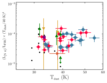
(a)

Figure 4: The distribution of $($L${}_{\textrm{\small\mbox{[N~{}{\sc ii}]}}}$/L${}_{\textrm{\small FIR}})\times($T${}_{\textrm{\small dust}}/40$ K$)^{4}$ versus T${}_{\textrm{\small dust}}$. We plot SPT SMGs in blue diamonds and red circles. Blue diamonds represent sources with L${}_{\textrm{\small\mbox{[C~{}{\sc ii}]}}}$/L${}_{\textrm{\small\mbox{[N~{}{\sc ii}]}}}$ $>10$, red circles represent L${}_{\textrm{\small\mbox{[C~{}{\sc ii}]}}}$/L${}_{\textrm{\small\mbox{[N~{}{\sc ii}]}}}$ $<10$. This allows us to investigate whether sources with more significant [N ii] emission exhibit a relationship between L${}_{\textrm{\small\mbox{[N~{}{\sc ii}]}}}/$L${}_{\textrm{\small FIR}}$ and dust temperature. The other souces utilize the same legend as Figure 3.

2 Sample selection, observations and data reduction

This sample of 40 gravitationally lensed SMGs are selected from the South Pole Telescope Sunyaev-Zeldovich (SPT-SZ) survey (Vieira et al. 2010, Mocanu et al. 2013) covering 2500 deg² at 3, 2, and 1.4 mm wavelengths. We selected a subset of sources with $3<z<6$ in order to enable observation of the [N ii] 205 $\mu$m line within bands 6 and 7 of ACA, including many sources which had existing [C ii] observations (e.g. Gullberg et al. 2015). Each source has a secure spectroscopic redshift (Table 1) determined primarily using CO transitions and other fine-structure lines (see Strandet et al. 2016 for details).

The [N ii] line observations for all sources were observed with ACA in Cycle 4 (PI: Chapman, 2016.1.00133.T), except for SPT2132–58 which was observed with the ALMA 12 m array (Béthermin et al. 2016). ACA is ideal for our measurements of the total [N ii] line flux from lensed sources with large (up to $\sim 1.5^{\prime\prime}$) Einstein radii because its FWHM beam size is 3 to 4$\arcsec$ at these frequencies, with the short observations typically yielding elongated beams due to restricted UV coverage. The ACA sensitivity is still sufficient to detect this relatively faint [N ii] line (compared to the much brighter [C ii]) in the gravitationally lensed SMGs. The [C ii] observations used here were taken with the single dish Atacama Pathfinder Experiment (APEX) and are described in detail in Gullberg et al. (2015).

The [N ii] data were reduced using the Common Astronomy Software Applications package (casa) version 4.7 (McMullin et al., 2007). casa’s clean function was used to generate continuum images and line cubes. The clean depth varied depending on the source, but was between 2 to 5$\sigma$. The typical pixel size was 1″ with beam semi-major (minor) axes of approximately 5 to 7″ (3 to 4)″. Our observations of [N ii] and [C ii] lines are shown in Figure 2. Our observations achieved RMS continuum noise of 0.5 to 0.9 mJy per beam.

Figure 1 illustrates continuum images of two of the most extended lensed SMGs in our sample, one from each of band 6 and 7, with high-resolution ALMA band 7 continuum contours superposed. This figure illustrates that our ACA observations are unresolved even for the largest sources. To test this assumption, we extracted both continuum and line flux from elliptical aperture regions corresponding to 1$\times$ and 1.5$\times$ the beam size, in addition to a point source, single pixel extraction. These aperture extractions did not alter (or increase) the line flux measurement, indicating complete flux contained within the extraction pixel. [N ii] spectral lines and the corresponding continuum were extracted at the peak of emission for all sources, with a single pixel extraction, and are shown in Figure 2 with integrated line fluxes and luminosities given in Table 1. The continuum emission is subtracted using a zeroth order polynomial matched to the flux baseline of off-line regions.

In Figure 2, we plot [N ii] , [C ii] , and either CO(5-4) or CO(4-3) from Strandet et al. (2016), depending on redshift. In order to most reliably determine the integrated fluxes in both [N ii] and [C ii], we use the FWHM${}_{\textrm{\small CO}}$ of the high signal-to-noise ratio (SNR) CO lines to determine the velocity range over which to sum our [N ii] and [C ii] detections. We first fit the CO line profiles with a single Gaussian function and then use this to obtain our line flux measurements by summing [N ii] and [C ii] over a velocity range $2\times$FWHM${}_{\textrm{\small CO}}$, covering the full-width of our [N ii] line profiles. For brighter [N ii] sources we confirmed through a curve of growth analysis that this represents $>95$% of the line flux, while for fainter [N ii] sources this avoids large variations in the line flux measurement from integrating noise fluctuations outside the line frequencies. For sources with both [N ii] and [C ii] observations, we compared the FWHM determined from a Gaussian fit for each line. Over the full sample, there is a good one-to-one agreement between these two line widths, although the relatively low SNRs of many of the lines (both [N ii] and [C ii]) result in significant scatter in the relation.

We fit the [N ii] line profiles and compare to the [C ii] profiles, both listed in Table 1. In 4 of the 40 cases, our spectral bandwidth only covers between 50% to 70% of the CO-defined line (SPT0125–50, SPT0300–46, SPT0243–49, and SPT0550–53). This was a compromise taken in order to attempt to reduce the overall project calibration overhead, since the total project exceeded 50 hours. In these cases, we only sum the [C ii] line to the end of the [N ii] line coverage. The [N ii] and [C ii] fluxes, along with the observed [N ii] luminosities are presented in Table 1. In Figure 3, the demagnified [N ii] luminosities are plotted against demagnified L${}_{\textrm{\small FIR}}$ and T${}_{\textrm{\small dust}}$, using magnification values ($\mu$) from Spilker et al. (2016).

3 Results

We robustly detect [N ii] lines with the ACA at $>4.5\sigma$ in 22 of our sample of 41 SMG observations (including SPT2132-58 from Béthermin et al. 2016), with a further 13 sources detected at $\geq 3\sigma$. The $>4.5\sigma$ criteria results in a 5% false positive chance in our data, which drops to less than 1% chance when the measurement is constrained to within one-half beam of the CO-source coordinates. These lines are detected at the redshifted velocity expected based on redshifts presented in Strandet et al. (2016). Along with the $11.5\sigma$ [N ii] detection of SPT2132–58 (Béthermin et al. 2016), this represents a total of 35 detections in the sample of 41. In the 6 sources with undetected [N ii], an upper limit was estimated as 3$\times$ the channel RMS in the central pixel at velocities away from the line. For our lines with $\sigma\geq 3$, we find magnified [N ii] line fluxes ranging between approximately $1$ to $14\textrm{~{}Jy km/s}$ and [C ii] flux between $5$ to $216\textrm{~{}Jy km/s}$. These correspond to [N ii] line luminosities of $(\sim 5$ to $40)\times 10^{8}$ L_⊙, and detected L${}_{\textrm{\small\mbox{[C~{}{\sc ii}]}}}$/L${}_{\textrm{\small\mbox{[N~{}{\sc ii}]}}}$ line luminosity ratios over two orders of magnitude. The sample has an interquartile range in line luminosity ratios L${}_{\textrm{\small\mbox{[C~{}{\sc ii}]}}}$/L${}_{\textrm{\small\mbox{[N~{}{\sc ii}]}}}$ of 5.0 to 24.7 and a median of 11.0 (see Figure 3, rightmost panel for a histogram detailing this distribution). These statistical values are calculated by treating the L${}_{\textrm{\small\mbox{[C~{}{\sc ii}]}}}$/L${}_{\textrm{\small\mbox{[N~{}{\sc ii}]}}}$ lower limits ([N ii] non-detections) as real measured values at the measured limit.

To properly account for the lower limits in L${}_{\textrm{\small\mbox{[C~{}{\sc ii}]}}}$/L${}_{\textrm{\small\mbox{[N~{}{\sc ii}]}}}$ , we perform survival analysis using the lifelines Python package (Davidson-Pilon et al., 2018). Survival analysis is often used to determine the time until an event occurs. In cases where an event is not precisely observed, the last observation made before the event occurs can still be used as a lower limit in calculating statistical quantities. For our line ratios, we utilize the lower limits as the last observation before the “event” occurs, where the event is the true line ratio. This analysis gives a slightly lower median value of 9.7 with a similar interquartile range of 5 to 25. Furthermore, reducing our sample to include only sources with good quality [N ii] and [C ii] detections did not significantly alter our measured medians or interquartile ranges.

In the majority of our sources ($17/30$, or $\sim$ 60 %), the L${}_{\textrm{\small\mbox{[C~{}{\sc ii}]}}}$/L${}_{\textrm{\small\mbox{[N~{}{\sc ii}]}}}$ luminosity ratio (or lower limit) corresponds to model expectations from XDR/PDR or shock regions determined by Decarli et al. (2014). Decarli et al. (2014) use L${}_{\textrm{\small\mbox{[C~{}{\sc ii}]}}}/$L${}_{\textrm{\small\mbox{[N~{}{\sc ii}]}}}\sim 2$ for H ii regions and greater than L${}_{\textrm{\small\mbox{[C~{}{\sc ii}]}}}/$L${}_{\textrm{\small\mbox{[N~{}{\sc ii}]}}}\sim 9$ for PDR/XDR regions (see Figure 3). Three SPT SMGs fall well within the range expected for H ii-dominated regions (with another 3 overlapping within error or as a lower limit), with the rest existing in an intermediate region, or more balanced regime in between the ionized gas dominated and PDR/shock dominated regions. Galaxies with [C ii]/[N ii] ratios in the XDR/PDR or shock region regime are expected to have [N ii] emission originating predominantly from H ii regions with [C ii] emission originating from both H ii regions and the outer layers of PDRs (Béthermin et al., 2016).

We assembled a sample of L${}_{\textrm{\small\mbox{[C~{}{\sc ii}]}}}$/L${}_{\textrm{\small\mbox{[N~{}{\sc ii}]}}}$ in local LIRGs from Díaz-Santos et al. (2017), Lu et al. (2017), and Zhao et al. (2016). To investigate whether the SPT SMG sample and the local LIRGs arise from different underlying distributions of L${}_{\textrm{\small\mbox{[C~{}{\sc ii}]}}}$/L${}_{\textrm{\small\mbox{[N~{}{\sc ii}]}}}$, we perform a two-sample KS test and T-test. The KS test yields a p-value of 0.44, while the T-test yields p $=0.36$. These test results prevent us from conclusively determining the line ratios come from different underlying distributions. In our literature sample, when dust temperatures were not available they were estimated using the relationship shown in Symeonidis et al. (2013).

We investigate the relationship between L${}_{\textrm{\small\mbox{[N~{}{\sc ii}]}}}/$L${}_{\textrm{\small FIR}}$ versus L${}_{\textrm{\small FIR}}$ (42.5 to 122.5 $\mu$m) by binning our sources according to L${}_{\textrm{\small FIR}}$. We divide our sources with L${}_{\textrm{\small\mbox{[N~{}{\sc ii}]}}}$ measurements into three bins of roughly equal size, ranging from log${}_{10}($L${}_{\textrm{\small FIR}})=$[$<$12.71, 12.71–12.9,$>$12.9$]$. From smallest to largest bins, we measure L${}_{\textrm{\small\mbox{[N~{}{\sc ii}]}}}/$L${}_{\textrm{\small FIR}}$ of $\sim 6.8\times 10^{-5}$, $4.3\times 10^{-5}$, and $3.0\times 10^{-5}$. These bins and their medians (and errors) are shown as black diamonds and grey shaded regions in the lower-left panel of Figure 3.

We also investigate the trend between dust temperature and L${}_{\textrm{\small\mbox{[N~{}{\sc ii}]}}}$/L${}_{\textrm{\small FIR}}$. These results are presented in the bottom-right panel of Figure 3, where we plot L${}_{\textrm{\small\mbox{[N~{}{\sc ii}]}}}$/L${}_{\textrm{\small FIR}}$ against T${}_{\textrm{\small dust}}$. We also bin our sources into 3 bins of roughly equal number according to dust temperature: T${}_{\textrm{\small dust}}=$[$<$39.3, 39.3–43.8, $>$43.8]. These bins have median values L${}_{\textrm{\small\mbox{[N~{}{\sc ii}]}}}$/L${}_{\textrm{\small FIR}}$ of $\sim 7.3\times 10^{-5}$, $3.1\times 10^{-5}$, and $3.0\times 10^{-5}$.

4 Discussion

Our [N ii] observations for a sample of 40 SMGs at $z=3-6$ represent the largest uniformly selected sample of high-redshift [N ii] detections to date. In our 30 sources with both [N ii] and [C ii] observations, we are able to characterize the L${}_{\textrm{\small\mbox{[C~{}{\sc ii}]}}}$/L${}_{\textrm{\small\mbox{[N~{}{\sc ii}]}}}$ out to the high-redshifts probed by our SMG sample, and in over a decade range in (de-magnified) far-IR luminosity ($\sim 12<\log_{10}($L${}_{\textrm{\sc fir}}/\mu)<13.5$). This has allowed us to capture the true L${}_{\textrm{\small\mbox{[C~{}{\sc ii}]}}}$/L${}_{\textrm{\small\mbox{[N~{}{\sc ii}]}}}$ range for luminous, dusty galaxies, and better understand the outliers to the distribution.

All previous literature measurements of L${}_{\textrm{\small\mbox{[C~{}{\sc ii}]}}}$/L${}_{\textrm{\small\mbox{[N~{}{\sc ii}]}}}$ in distant, far-IR luminous galaxies are found to lie within the range of L${}_{\textrm{\small\mbox{[C~{}{\sc ii}]}}}$/L${}_{\textrm{\small\mbox{[N~{}{\sc ii}]}}}$ ratios we observe in the SPT SMGs. The SPT SMGs exhibit among the highest and lowest ratios yet seen in high-redshift, FIR luminous galaxies. However, our measurements also detect a population of high-redshift SMGs which have lower L${}_{\textrm{\small\mbox{[C~{}{\sc ii}]}}}$/L${}_{\textrm{\small\mbox{[N~{}{\sc ii}]}}}$ ratios than shown in previous literature. We find 8 of our 30 SMGs have L${}_{\textrm{\small\mbox{[C~{}{\sc ii}]}}}$/L${}_{\textrm{\small\mbox{[N~{}{\sc ii}]}}}$ values (or are consistent within error) suggesting a hybrid regime between the model predictions of PDR/XDR emission and H ii regions. These sources suggest neither H ii regions nor PDR/XDR regions dominate the [C ii] flux. Instead the [C ii] flux has significant contributions from both regions. The L${}_{\textrm{\small\mbox{[C~{}{\sc ii}]}}}$/L${}_{\textrm{\small\mbox{[N~{}{\sc ii}]}}}$ in these sources cannot be explained as originating in only H ii regions – both neutral and ionized gas must contribute to the total [C ii] 158 $\mu$m luminosity. SMGs lying in this hybrid or even H ii dominated regimes could represent very enriched, high-metallicity gas in combination with low gas densities, and appropriate ionization parameters. The C/N abundance ratio may vary as a function of metallicity (e.g. Nagao et al. 2012), and could be an important contributor to the L${}_{\textrm{\small\mbox{[C~{}{\sc ii}]}}}$/L${}_{\textrm{\small\mbox{[N~{}{\sc ii}]}}}$ line ratio. These SMGs may also have very high masses of ionized gas relative to the molecular gas fraction. Detailed multi-line studies of these sources will be undertaken in follow-up contributions to better understand this unusual situation for such massive and dusty star-forming galaxies.

At the highest values of L${}_{\textrm{\small\mbox{[C~{}{\sc ii}]}}}$/L${}_{\textrm{\small\mbox{[N~{}{\sc ii}]}}}$ we detect 5 sources with larger ratios than the previous SMG record holder SPT2132–58 (Béthermin et al., 2016), and comparable to the lower far-IR luminous sources of Umehata et al. (2017) and Pavesi et al. (2016). These sources likely represent extreme ISM environments, where total [C ii] emission is dominated by the contribution from PDR/XDR regions. Since neutral nitrogen has a higher ionization potential than hydrogen, we expect that [N ii] 205 $\mu$m emission will only originate in ionized gas. Therefore, our sources with extremely high L${}_{\textrm{\small\mbox{[C~{}{\sc ii}]}}}$/L${}_{\textrm{\small\mbox{[N~{}{\sc ii}]}}}$ may have a relatively low contribution to [C ii] from ionized gas where the [N ii] originates.

Comparing our SMG sample to local LIRGs, we observe slightly higher L${}_{\textrm{\small\mbox{[C~{}{\sc ii}]}}}$/L${}_{\textrm{\small\mbox{[N~{}{\sc ii}]}}}$ values, possibly owing to lower density gas and therefore a lower contribution of [C ii] emission from PDR/XDR regions in local (U)LIRGs. However, the p-values from both the T-test and KS-test (see Section 3) suggest we cannot say the SMGs and local LIRGs arise from different underlying distributions.

We follow the analysis of Nagao et al. (2012) and include two metallicity grids for gas densities of $\log(n)=1.5$ and $=3$, each with ionization parameter $\log(U)=-3.5$ in Figure 3. According to the models of Nagao et al. (2012), higher L${}_{\textrm{\small\mbox{[C~{}{\sc ii}]}}}$/L${}_{\textrm{\small\mbox{[N~{}{\sc ii}]}}}$ should originate in lower metallicity environments. In our sample, we see that the majority of our sample of galaxies have line ratios that place them in the metallicity range of $0.6<Z/Z_{\odot}<3.0$ if we assume the $\log(n)=3$. Assuming $\log(n)=1.5$, we find metallicities in the range $0.2<Z/Z_{\odot}<1.0$. In both cases, the metallicity spans sub- to solar or super-solar ranges. However, direct interpretation of L${}_{\textrm{\small\mbox{[C~{}{\sc ii}]}}}$/L${}_{\textrm{\small\mbox{[N~{}{\sc ii}]}}}$ in terms of metallicity is undermined by unconstrained gas density, elemental abundances, fractional abundance of ionized and neural gas, and ionization parameter, which can also affect this luminosity ratio (e.g. Nagao et al. 2012, Pavesi et al. 2016). In galaxies with a significant fraction of neutral ISM, [C ii] emission will more heavily out-weigh [N ii] than in galaxies with a significant ionized ISM component.

We investigate the relationship between L${}_{\textrm{\small\mbox{[N~{}{\sc ii}]}}}$/L${}_{\textrm{\small FIR}}$ versus T${}_{\textrm{\small dust}}$. We observe a deficit in L${}_{\textrm{\small\mbox{[N~{}{\sc ii}]}}}$/L${}_{\textrm{\small FIR}}$ towards higher T${}_{\textrm{\small dust}}$ after binning according to dust temperature. Gullberg et al. (2015) similarly observed decreasing L${}_{\textrm{\small\mbox{[C~{}{\sc ii}]}}}$/L${}_{\textrm{\small FIR}}$ towards increasing dust temperature. This result was first presented and explained in Malhotra et al. (2001) who explained this ratio may change due to one of two reasons: (1) high far ultraviolet flux to gas density ratios may positively charge dust grains and therefore decrease heating efficiency, or (2) softer radiation fields can be less effective in heating gas and instead heat only the dust. Gullberg et al. (2015) acknowledged the Stefan-Boltzmann law may explain part of this dependence, as L${}_{\textrm{\small FIR}}\propto$ T${}_{\textrm{\small dust}}^{4}$. To cancel this relationship, we plot $($L${}_{\textrm{\small\mbox{[N~{}{\sc ii}]}}}$/L${}_{\textrm{\small FIR}})\times($T${}_{\textrm{\small dust}}/40$ K$)^{4}$ versus T${}_{\textrm{\small dust}}$ in Figure 4. After removing this dependence, we perform a Kendall Tau test on the sample and calculate a p-value of 0.49. Similarly to the results presented in Gullberg et al. (2015), this result means we neither confirm the existence of a correlation between these variables, nor that [N ii] emission is largely independent of dust temperature for our SPT SMGs. To investigate whether the trend appears in sources depending on the relative significance of [N ii] emission, we reduce the sample into two sub-samples according to their L${}_{\textrm{\small\mbox{[C~{}{\sc ii}]}}}$/L${}_{\textrm{\small\mbox{[N~{}{\sc ii}]}}}$. We define the [N ii] significant sources as those with L${}_{\textrm{\small\mbox{[C~{}{\sc ii}]}}}$/L${}_{\textrm{\small\mbox{[N~{}{\sc ii}]}}}$$<10$, and the [N ii] insignificant sources with L${}_{\textrm{\small\mbox{[C~{}{\sc ii}]}}}$/L${}_{\textrm{\small\mbox{[N~{}{\sc ii}]}}}$$>10$. For these samples, we repeat the Kendall Tau test and calculate p-values of 0.17 and 0.08, respectively. This indicates our sources with significant ionized gas emission L${}_{\textrm{\small\mbox{[C~{}{\sc ii}]}}}$/L${}_{\textrm{\small\mbox{[N~{}{\sc ii}]}}}$$<10$ do not exhibit a correlation between L${}_{\textrm{\small\mbox{[N~{}{\sc ii}]}}}$/L${}_{\textrm{\small FIR}}$ and T${}_{\textrm{\small dust}}$, nor do sources with more significant PDR/XDR region emission.

5 Conclusions

We have presented the first uniformly selected sample of high-redshift [N ii] 205 $\mu$m observations and utilized previous observations of the [C ii] 158 $\mu$m line to probe the ISM. We summarize our main conclusions here:

• We find that our SPT SMGs have a wide distribution of L${}_{\textrm{\small\mbox{[C~{}{\sc ii}]}}}$/L${}_{\textrm{\small\mbox{[N~{}{\sc ii}]}}}$. The median L${}_{\textrm{\small\mbox{[C~{}{\sc ii}]}}}$/L${}_{\textrm{\small\mbox{[N~{}{\sc ii}]}}}$ is 11.0 with an interquartile range of 5.0 to 24.7. Using survival statistics to account for our lower limits did not significantly alter our results. This resulted in a median of 9.7 and an interquartile range of 5 to 25.

• We measure a decrease in L${}_{\textrm{\small\mbox{[N~{}{\sc ii}]}}}$/L${}_{\textrm{\small FIR}}$ towards increasing L${}_{\textrm{\small FIR}}$. From the lowest luminosity bin (log${}_{10}($L${}_{\textrm{\small FIR}})<12.71$) to our highest luminosity bin (log${}_{10}($L${}_{\textrm{\small FIR}})>12.9$) we find medians of $\sim 1.6\times 10^{-4}$ decreasing to $\sim 1.2\times 10^{-4}$.

• We cannot determine whether our measured [N ii] emission is independent of dust temperature, after cancelling the L${}_{\textrm{\small FIR}}\propto$ T${}_{\textrm{\small dust}}^{4}$ dependence and performing a Kendall Tau correlation test, including samples with high and low L${}_{\textrm{\small\mbox{[C~{}{\sc ii}]}}}$/L${}_{\textrm{\small\mbox{[N~{}{\sc ii}]}}}$ values.

• Our range in observed L${}_{\textrm{\small\mbox{[C~{}{\sc ii}]}}}$/L${}_{\textrm{\small\mbox{[N~{}{\sc ii}]}}}$ can be explained through variations in gas density, ionization parameter, and metallicity. We note that further observations of fine-structure lines such as [N ii] 122 $\mu$m and [O i] 145 $\mu$m will help break the degeneracy of the L${}_{\textrm{\small\mbox{[C~{}{\sc ii}]}}}$/L${}_{\textrm{\small\mbox{[N~{}{\sc ii}]}}}$ on gas density and ionization parameter (Nagao et al. 2012), and will help strengthen conclusions based on comparisons of the [C ii]-to-[N ii] ratio between local LIRGs and the high-redshift universe.

Table 1: Observed properties for our 41 SMGs ordered by $\mu$ S${}_{\textrm{\small\mbox{[N~{}{\sc ii}]}}}$, the observed line flux without gravitational lensing correction. The [N ii] properties are determined from a single pixel extracted [N ii] spectra. The instrinic flux is determined by dividing the observed flux by the gravitational lensing factor $\mu$. Redshifts are provided from Strandet et al. (2016), while lensing models and $\mu$ values can be found in Spilker et al. (2016). For sources without lensing models, we assume our median magnification of $\mu=6.3$ for strongly lensed SMGs (Spilker et al., 2016). Sources with model magnifications close to or equal to one are likely unlensed systems, some suspected to be the cores of dense protoclusters (e.g. Miller et al. 2018). Sources without a FWHM listed in the [C ii] column do not have [C ii] observations. Sources without a FWHM listed in the [N ii] column have line profiles too noisy to reliably fit with a gaussian function.

Source	$z$	$\mu$ S${}_{\textrm{\small\mbox{[N~{}{\sc ii}]}}}{}^{a}$	SNR${}_{\textrm{\small\mbox{[N~{}{\sc ii}]}}}{}^{b}$	$\mu$ L${}_{\textrm{\small\mbox{[N~{}{\sc ii}]}}}$	$\mu$ S${}_{\textrm{\small\mbox{[C~{}{\sc ii}]}}}$	FWHM${}_{\textrm{\small\mbox{[N~{}{\sc ii}]}}}$	FWHM${}_{\textrm{\small\mbox{[C~{}{\sc ii}]}}}$	$\mu$
		(Jy km s-1)		($\times$108 $L_{\odot}$)	(Jy km s-1)	(km s-1)	(km s-1)
0529-54	3.3689	13.6 $\pm$ 1.7	9.3	40.4 $\pm$ 5.0	64.6 $\pm$ 7.7	415 $\pm$ 44	733 $\pm$ 81	13.2 $\pm$ 0.8
0103-45	3.0917	12.1 $\pm$ 2.3	11.7	31.2 $\pm$ 5.9	190.4 $\pm$ 23.8	429 $\pm$ 67	239 $\pm$ 39	5.1 $\pm$ 0.1
0155-62	4.349	11.6 $\pm$ 1.0	5.7	51.6 $\pm$ 4.5	26.3 $\pm$ 6.2	732 $\pm$ 104	760 $\pm$ 127	6.3 $\pm$ 1.0f
2146-55	4.5672	9.3 $\pm$ 0.7	12.7	44.6 $\pm$ 3.4	11.3 $\pm$ 5.8	442 $\pm$ 55	277 $\pm$ 73	6.6 $\pm$ 0.4
0113-46	4.2328	9.1 $\pm$ 0.5	8.7	38.8 $\pm$ 2.1	49.7 $\pm$ 12.8	616 $\pm$ 65	578 $\pm$ 136	23.9 $\pm$ 0.5
0532-50	3.3988	9.0 $\pm$ 0.8	7.3	27.1 $\pm$ 2.4	91.7 $\pm$ 11.2	755 $\pm$ 123	719 $\pm$ 125	10.0 $\pm$ 0.6
2357-51	3.0703	8.7 $\pm$ 1.1	7.3	22.2 $\pm$ 2.8	9.1 $\pm$ 4.6	692 $\pm$ 129	743 $\pm$ 202	2.9 $\pm$ 0.1
2037-65	4.000	8.4 $\pm$ 0.7	8.1	32.8 $\pm$ 2.7	—	503 $\pm$ 76	—	6.3 $\pm$ 1.0f
0109-47	3.6137	8.1 $\pm$ 1.8	9.1	26.9 $\pm$ 6.0	—	545 $\pm$ 75	—	10.2 $\pm$ 1.0
2147-50	3.7602	7.9 $\pm$ 0.6	9.1	28.0 $\pm$ 2.1	24.4 $\pm$ 7.5	570 $\pm$ 63	534 $\pm$ 104	6.6 $\pm$ 0.4
0020-51	4.1228	7.5 $\pm$ 0.6	9.4	30.7 $\pm$ 2.5	—	459 $\pm$ 66	—	4.2 $\pm$ 0.1
0027-50	3.4436	7.3 $\pm$ 0.9	8.2	22.5 $\pm$ 2.8	—	288 $\pm$ 38	—	5.1 $\pm$ 0.2
0418-47	4.2248	7.2 $\pm$ 0.6	12.5	30.6 $\pm$ 2.6	138.1 $\pm$ 10.4	366 $\pm$ 35	322 $\pm$ 37	32.7 $\pm$ 0.7
2103-60	4.4357	5.8 $\pm$ 0.6	8.7	26.6 $\pm$ 2.8	15.6 $\pm$ 10.4	670 $\pm$ 110	602 $\pm$ 204	27.8 $\pm$ 1.8
0459-59	4.7993	5.5 $\pm$ 0.8	8.2	28.5 $\pm$ 4.1	—	464 $\pm$ 63	—	4.2 $\pm$ 0.4
0551-50	3.164	5.2 $\pm$ 1.3	5.9	13.9 $\pm$ 3.5	216.1 $\pm$ 16.3	775 $\pm$ 273	734 $\pm$ 95	4.5 $\pm$ 0.5c
2101-60	3.156	5.0 $\pm$ 1.8	6.0	13.3 $\pm$ 4.8	9.3 $\pm$ 13.8	682 $\pm$ 273	353 $\pm$ 189	6.3 $\pm$ 1.0f
0136-63	4.299	4.8 $\pm$ 0.7	3.8	21.0 $\pm$ 3.1	33.3 $\pm$ 2.9	500 $\pm$ 128	526 $\pm$ 115	6.3 $\pm$ 1.0f
0125-50d	3.959	4.7 $\pm$ 0.9	4.2	18.1 $\pm$ 3.5	—	—	—	14.1 $\pm$ 0.5
0345-47	4.2958	4.4 $\pm$ 0.7	4.9	19.2 $\pm$ 3.1	15.4 $\pm$ 4.3	350 $\pm$ 75	669 $\pm$ 177	8.0 $\pm$ 0.5
2048-55	4.089	4.4 $\pm$ 1.1	3.0	17.8 $\pm$ 4.4	—	472 $\pm$ 156	—	6.3 $\pm$ 0.7
0550-53d	3.128	4.2 $\pm$ 1.4	4.5	11.0 $\pm$ 3.7	88.1 $\pm$ 8.6	—	789 $\pm$ 165	6.3 $\pm$ 1.0f
0459-58	4.856	4.1 $\pm$ 0.7	4.0	21.6 $\pm$ 3.7	—	525 $\pm$ 143	—	5.0 $\pm$ 0.6
2311-54	4.2795	3.6 $\pm$ 0.6	3.9	15.6 $\pm$ 2.6	45.3 $\pm$ 4.6	315 $\pm$ 129	352 $\pm$ 52	6.3 $\pm$ 1.0f
0243-49d	5.699	3.3 $\pm$ 0.9	3.9	22.1 $\pm$ 6.0	17.4 $\pm$ 2.7	—	796 $\pm$ 202	6.7 $\pm$ 0.5
0348-62	5.656	3.0 $\pm$ 0.6	4.8	19.9 $\pm$ 4.0	19.6 $\pm$ 3.4	507 $\pm$ 213	506 $\pm$ 132	1.2 $\pm$ 0.01
2340-59	3.864	2.6 $\pm$ 0.5	4.5	9.6 $\pm$ 1.8	48.1 $\pm$ 8.5	579 $\pm$ 198	473 $\pm$ 220	3.4 $\pm$ 0.3
0516-59	3.4045	2.6 $\pm$ 0.8	3.8	7.9 $\pm$ 2.4	—	156 $\pm$ 254	—	6.3 $\pm$ 1.0f
0245-63	5.626	2.4 $\pm$ 0.2	2.9	15.8 $\pm$ 1.3	26.9 $\pm$ 4.5	241 $\pm$ 83	383 $\pm$ 65	1.0 $\pm$ 0.01
2353-50	5.576	2.2 $\pm$ 0.3	2.6	14.3 $\pm$ 1.9	20.7 $\pm$ 6.4	613 $\pm$ 405	429 $\pm$ 247	6.3 $\pm$ 1.0f
0300-46d	3.5954	2.1 $\pm$ 1.2	4.2	6.9 $\pm$ 4.0	15.7 $\pm$ 5.1	—	414 $\pm$ 237	5.7 $\pm$ 0.4
2319-55	5.2929	2.0 $\pm$ 0.8	3.9	12.0 $\pm$ 4.8	39.2 $\pm$ 4.7	339 $\pm$ 245	176 $\pm$ 28	6.9 $\pm$ 0.6
0319-47	4.51	2.0 $\pm$ 0.5	3.5	9.4 $\pm$ 2.4	11.4 $\pm$ 10.5	259 $\pm$ 42	562 $\pm$ 182	2.9 $\pm$ 0.3
2307-50	3.105	1.9 $\pm$ 0.6	3.2	4.9 $\pm$ 1.6	—	$\sim 98$	—	6.3 $\pm$ 1.0f
2132-58e	4.7677	1.7 $\pm$ 0.2	11.5	8.9 $\pm$ 0.8	35.9 $\pm$ 6.9	245 $\pm$ 16	212 $\pm$ 43	5.7 $\pm$ 0.5
0441-46	4.4771	1.5 $\pm$ 0.5	2.9	7.0 $\pm$ 2.3	26.3 $\pm$ 5.8	393 $\pm$ 106	546 $\pm$ 123	12.7 $\pm$ 1.0
2349-56	4.304	1.1 $\pm$ 0.5	2.9	4.8 $\pm$ 2.2	—	—	—	1.0
0202-61	5.018	0.036g	4.5	—	19.3 $\pm$ 4.1	$\sim 60$	771 $\pm$ 325	9.1 $\pm$ 0.07
0346-52	5.6559	$>$0.9	2.9	$>$6.0	64.1 $\pm$ 8.2	$\sim 64$	486 $\pm$ 85	5.6 $\pm$ 0.1
2052-56	4.257	0.1 $\pm$ 0.4	2.3	0.4 $\pm$ 1.7	14.6 $\pm$ 1.8	$\sim 91$	382 $\pm$ 122	1.0
2351-57	5.811	$>$-0.8	2.7	$>$-5.5	5.4 $\pm$ 2.7	383 $\pm$ 409	539 $\pm$ 82	6.3 $\pm$ 1.0f

^a Errors quoted are RMS from the 1D spectra.
^b SNR determined from the source peak in uv-plane continuum subtracted channel maps.
^c Lens model by K. Sharon, private communication.
^d The [N ii] spectra for these sources does not have sufficient baseline to completely cover the CO line profile. The fluxes quoted for [N ii] and [C ii] are truncated to the [N ii] spectral coverage.
^e from Béthermin et al. (2016).
^f $\mu=6.3$ is assumed. No lensing model.
^g Positive flux measurement from channel map (Jy/beam). Our procedure for measuring total flux results in a negative value for this source.

References

- Aravena et al. (2016) Aravena M., et al., 2016, MNRAS, 457, 4406
- Béthermin et al. (2016) Béthermin M., et al., 2016, A&A, 586, L7
- Casey et al. (2014) Casey C. M., Narayanan D., Cooray A., 2014, Physics Reports, 541, 45
- Chapman et al. (2003) Chapman S. C., Blain A. W., Ivison R. J., Smail I. R., 2003, Nature, 422, 695 EP
- Chapman et al. (2005) Chapman S. C., Blain A. W., Smail I., Ivison R. J., 2005, ApJ, 622, 772
- Cormier et al. (2015) Cormier D., et al., 2015, A&A, 578, A53
- Cowley et al. (2017) Cowley W. I., Béthermin M., Lagos C. d. P., Lacey C. G., Baugh C. M., Cole S., 2017, MNRAS, 467, 1231
- Davidson-Pilon et al. (2018) Davidson-Pilon C., et al., 2018, CamDavidsonPilon/lifelines: v0.14.6, doi:10.5281/zenodo.1303381
- Decarli et al. (2014) Decarli R., et al., 2014, ApJL, 782, L17
- Díaz-Santos et al. (2017) Díaz-Santos T., et al., 2017, ApJ, 846, 32
- Ferland et al. (1998) Ferland G. J., Korista K. T., Verner D. A., Ferguson J. W., Kingdon J. B., Verner E. M., 1998, Publications of the Astronomical Society of the Pacific, 110, 761
- Gullberg et al. (2015) Gullberg B., et al., 2015, MNRAS, 449, 2883
- Hainline et al. (2011) Hainline L. J., Blain A. W., Smail I., Alexander D. M., Armus L., Chapman S. C., Ivison R. J., 2011, ApJ, 740, 96
- Hayward et al. (2013) Hayward C. C., Narayanan D., Kereš D., Jonsson P., Hopkins P. F., Cox T. J., Hernquist L., 2013, MNRAS, 428, 2529
- Herrera-Camus et al. (2016) Herrera-Camus R., et al., 2016, ApJ, 826, 175
- Lu et al. (2017) Lu N., et al., 2017, ApJSS, 230, 1
- Ma et al. (2015) Ma J., et al., 2015, ApJ, 812, 88
- Malhotra et al. (2001) Malhotra S., et al., 2001, The Astrophysical Journal, 561, 766
- McMullin et al. (2007) McMullin J. P., Waters B., Schiebel D., Young W., Golap K., 2007, in Shaw R. A., Hill F., Bell D. J., eds, Astronomical Society of the Pacific Conference Series Vol. 376, ADASS XVI. p. 127
- Michalowski, M. J. et al. (2012) Michalowski, M. J. Dunlop, J. S. Cirasuolo, M. Hjorth, J. Hayward, C. C. Watson, D. 2012, A&A, 541, A85
- Miller et al. (2018) Miller T. B., et al., 2018, Nature, 556, 469
- Mocanu et al. (2013) Mocanu L. M., et al., 2013, ApJ, 779, 61
- Nagao et al. (2012) Nagao T., Maiolino R., De Breuck C., Caselli P., Hatsukade B., Saigo K., 2012, A&A, 542, L34
- Narayanan et al. (2015) Narayanan D., et al., 2015, Nature, 525, 496 EP
- Oberst et al. (2006) Oberst T. E., et al., 2006, ApJL, 652, L125
- Pavesi et al. (2016) Pavesi R., et al., 2016, ApJ, 832, 151
- Pavesi et al. (2018) Pavesi R., Riechers D. A., Faisst A. L., Stacey G. J., Capak P. L., 2018, arXiv
- Rawle et al. (2014) Rawle T. D., et al., 2014, ApJ, 783, 59
- Riechers et al. (2014) Riechers D. A., et al., 2014, ApJ, 796, 84
- Shimizu et al. (2012) Shimizu I., Yoshida N., Okamoto T., 2012, Monthly Notices of the Royal Astronomical Society, 427, 2866
- Spilker et al. (2016) Spilker J. S., et al., 2016, ApJ, 826, 112
- Strandet et al. (2016) Strandet M. L., et al., 2016, ApJ, 822, 80
- Swinbank et al. (2014) Swinbank A. M., et al., 2014, MNRAS, 438, 1267
- Symeonidis et al. (2013) Symeonidis M., et al., 2013, Monthly Notices of the Royal Astronomical Society, 431, 2317
- Tadaki et al. (2019) Tadaki et al., 2019, The Astrophysical Journal, 876, 1
- Umehata et al. (2017) Umehata H., et al., 2017, ApJL, 834, L16
- Vieira et al. (2010) Vieira J. D., et al., 2010, ApJ, 719, 763
- Vieira et al. (2013) Vieira J. D., et al., 2013, Nature, 495, 344 EP
- Wardlow et al. (2011) Wardlow J., et al., 2011, Monthly Notices of the Royal Astronomical Society, 415, 1479
- Weiß et al. (2013) Weiß A., et al., 2013, ApJ, 767, 88
- Zhao et al. (2016) Zhao Y., et al., 2016, ApJ, 819, 69