Brain-Network Clustering via
Kernel-ARMA Modeling and the Grassmannian

Abstract

Recent advances in neuroscience and in the technology of functional magnetic resonance imaging (fMRI) and electro-encephalography (EEG) have propelled a growing interest in brain-network clustering via time-series analysis. Notwithstanding, most of the brain-network clustering methods revolve around state clustering and/or node clustering (a.k.a. community detection or topology inference) within states. This work answers first the need of capturing non-linear nodal dependencies by bringing forth a novel feature-extraction mechanism via kernel autoregressive-moving-average modeling. The extracted features are mapped to the Grassmann manifold (Grassmannian), which consists of all linear subspaces of a fixed rank. By virtue of the Riemannian geometry of the Grassmannian, a unifying clustering framework is offered to tackle all possible clustering problems in a network: Cluster multiple states, detect communities within states, and even identify/track subnetwork state sequences. The effectiveness of the proposed approach is underlined by extensive numerical tests on synthetic and real fMRI/EEG data which demonstrate that the advocated learning method compares favorably versus several state-of-the-art clustering schemes.

I Introduction

Recent advances in neuroscience reveal the brain to be a complex network capable of integrating and generating information from external and internal sources in real time [1]. The rapidly growing field of Network Neuroscience uses network analytics to reveal, via graph theory and its concepts (e.g., nodes and edges), topological and functional dependencies of the brain [2]. At the microscopic scale, nodes of a brain network correspond to individual neurons, while edges might describe synaptic coupling between neurons or relationships between their firing patterns [3]. At the macroscopic scale, nodes might be brain regions, and edges might represent anatomical connections (structural connectivity) or statistical relationships between regional brain dynamics (functional connectivity) [4].

Popular noninvasive techniques used to acquire time series data from brain networks include functional magnetic resonance imaging (fMRI) and electro-encephalography (EEG). In particular, fMRI monitors the blood oxygen-level dependent (BOLD) time series [5], while EEG tracks brain activity through the time series which are collected via electrodes on the scalp. EEG possesses a high temporal resolution and is considered to be relatively convenient, inexpensive, and harmless compared to other methods such as magneto-encephalography (MEG), which is much less risky than positron emission tomography (PET) [6].

An important aspect of the majority of works in network analytics is that the time-series data describing the nodal signals tend to be considered stationary, and many learning algorithms make the temporal smoothness assumption [7, 8]. However, stationarity of the brain network data should not be assumed, as it is known that the brain acts as a non-stationary network even during its resting state, e.g., [9, 10, 11, 12, 13]. Dynamic functional brain networks can be built using pairwise relationships derived from the time series data described above, and this dynamic-network viewpoint has been widely exploited to identify diseases, cognitive states, and individual differences in performance [14, 15, 16, 17].

Learning algorithms are often employed to identify functional dependencies among nodes and topology in networks. As a prominent example, clustering algorithms have been already utilized to verify the dynamic nature of brain networks [9, 10], as well as to predict and detect brain disorders, applied to syndromes at large, such as depression [18], epilepsy, schizophrenia [19], Alzheimer disease and autism [20]. In general, brain-network clustering methods aim at three major goals: Node clustering (a.k.a. community detection or topology inference) within a given brain state, state clustering of similar brain states, and subnetwork-state-sequence identification. Loosely speaking, a “brain state” corresponds to a specific “global” network topology or nodal connectivity pattern which stays fixed over a time interval. A “subnetwork state sequence” is defined as the latent (stochastic) process that drives a subnetwork/subgroup of nodal time series, may span several network-wide/“global” states, and the collaborating nodes may even change as the brain transitions from one “global” state to another.

Most brain-clustering algorithms are used for nodal and state clustering, while only very few schemes try to identify/track subnetwork state sequences. For example, community detection in brain networks has been studied extensively to perform clustering in both static and dynamic brain networks [21, 22]. Modularity maximization [23, 24] is a popular method for performing community detection in functional brain networks, but also relies on the selection of additional parameters determining the proper null model, resolution of clustering and in the dynamic case, the value of interlayer coupling [25]. In [26, 27], the discrete wavelet transform decomposes EEG signals into frequency sub-bands, and K-means is used to cluster the acquired wavelet coefficients. In [28], non-parametric Bayesian models, coined Bayesian community detection and infinite relational modeling, are introduced and applied to resting state fMRI data to define probabilities on network edges. Clustering in [28] is performed by running sophisticated comparisons on the values of those edge probabilities. Study [29] investigated network “motifs,” defined as recurrent and statistically significant sub-graphs or patterns. A spectral-clustering based algorithm applied to motif features revealed a spatially coherent, yet frequency dependent, sub-division between the posterior, occipital and frontal brain regions [29]. Entropy maximization and frequency decomposition were utilized in [30] prior to applying vector quantization [31] to frequency-based features for clustering communities within EEG data. In [32], EEG-data topography via Renyi’s entropy was proposed as a feature extraction mapping, before applying self-organizing maps as the off-the-shelf clustering algorithm. In the recently popular graph-signal-processing context [8, 33], topology inference is achieved by solving optimization problems formed via the observed time-series data and the eigen-decomposition of the Laplacian matrix of the network.

Other approaches have been used to perform state clustering. For example, [34] advocates hidden Markov models (HMMs) to characterize brain-state dynamics. HMM parameters are extracted from each state and used to form vectors in a Euclidean space, with their pairwise metric distances comprising the entries of an affinity matrix. Hierarchical clustering is then applied to the affinity matrix to cluster brain states. In [35], time-varying features are extracted from healthy controls and patients with schizophrenia using independent vector analysis (IVA). Mutual information among the IVA features, Markov modeling and K-means are used to detect changes in the brain’s spatial connectivity patterns. A change-point detection approach for resting state fMRI is introduced in [36]. Functional connectivity patterns of all fiber-connected cortical voxels are concatenated into a descriptive feature vector to represent the brain’s state, and the temporal change points of different brain states are decided by detecting the abrupt changes of the vector patterns via a sliding window approach. In [37], hierarchical clustering is applied to a time series of graph-distance measures to identify discrete states of networks. Moreover, motivated by the observation that changes in nodal communities suggest changes in network states, studies [38, 39] perform community detection on fMRI data, prior to state clustering, by capitalizing on K-means, multi-layer modeling, (Tucker) tensor and higher-order singular value decomposition.

There is only a few methods that can cluster subnetwork state sequences in fMRI and EEG modalities. In [40], features are extracted from the frequency content of the fMRI/EEG time series. A feature example is the ratio of the sum of amplitudes within a specific frequency interval over the sum of amplitudes over the whole frequency range of the time series. Features, and thus subnetwork state sequences, are then clustered via K-means [40]. A computer-vision approach is introduced in [41]. EEG data are transformed into dynamic topographic maps, able to display features such as voltage amplitude, power and peak latency. The flow of activation within those topographic maps is estimated by using an optical-flow estimation method [42] which generates motion vectors. Motion vectors are clustered into groups, and these dynamic clusters are tracked along the time axis to depict the activation flow and track the subnetwork state sequences.

This paper capitalizes on the directions established by [43] to introduce a unifying feature-extraction and clustering framework, with strong geometric flavor, that make no assumptions of stationarity and can carry through all possible brain-clustering duties, i.e., community detection, state clustering, and subnetwork-state-sequence clustering/tracking. A kernel autoregressive-moving-average (K-ARMA) model is proposed to capture latent non-linear and causal dependencies, not only within a single time series, but also among multiple nodal time series of the brain network. To accommodate the highly likely non-stationarity of the time series, the K-ARMA model is applied via a time-sliding window. Per application of the K-ARMA model, a system identification problem is solved to extract a low-rank observability matrix. Such a low-rank representation enables dimensionality-reduction arguments which are beneficial to learning methods for the usually high-dimensional ambient spaces associated with brain-network analytics. Features are defined as the low-rank column spaces of the computed observability matrices. For a fixed rank, those features become points of the Grassmann manifold (Grassmannian), which enjoys the rich Riemannian geometry. This feature-extraction scheme permeates all clustering duties in this study. Having obtained the features and to identify clusters, this study builds on Riemannian multi-manifold modeling (RMMM) [44, 45, 43], which postulates that clusters take the form of sub-manifolds in the Grassmannian. To compute clusters, the underlying Riemannian geometry is exploited by the geodesic-clustering-with-tangent-spaces (GCT) algorithm [44, 45, 43]. Unlike the pipeline in [46], which used covariance matrix of EEG, after low-pass filtering, as feature on a manifold and considered only the Riemannian distance between features, GCT considers both distance and angle as geometric information for clustering. In contrast to [44, 45, 43], where the number of clusters need to be known a priori, this paper incorporates hierarchical clustering to render GCT free from any a-priori knowledge of the number of clusters. Extensive numerical tests on synthetic and real fMRI/EEG data demonstrate that the proposed framework, i.e., feature extraction mechanism and GCT-based clustering algorithm, compares favorably versus state-of-the-art manifold learning and brain-network clustering schemes.

The rest of the paper is organized as follows. The K-ARMA model and the feature-extraction mechanism are introduced in Section II. The new variant of the GCT clustering algorithm is presented in Section III, while synthetic and real fMRI/EEG data are used in Section IV to validate the theoretical and algorithmic developments. The manuscript is concluded in Section V, while mathematical notation, any background material as well as proofs are deferred to the Appendix.

II Kernel-ARMA Modeling

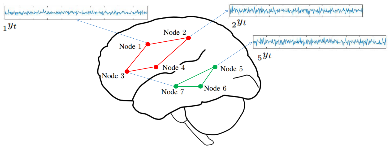
Figure 1: Brain network with nodes, edges, and nodal time series (signals) $\prescript{}{\nu}{y}_{t}$.

Consider a (brain) network/graph $\mathcal{G}\coloneqq(\mathcal{N},\mathcal{E})$, with sets of nodes $\mathcal{N}$, of cardinality $\lvert\mathcal{N}\rvert$, and edges $\mathcal{E}$. Each node $\nu\in\mathcal{N}$ is annotated by a discrete-time stochastic process (time series) $(\prescript{}{\nu}{y}_{t})_{t\in\mathbb{Z}}$, where $t$ denotes discrete time and $\mathbb{Z}$ the set of all integer numbers; cf. Fig. 1. To avoid congestion in notations, $\prescript{}{\nu}{y}_{t}$ stands for both the random variable (RV) and its realization. The physical meaning of $\mathcal{N}$ and $(\prescript{}{\nu}{y}_{t})_{t\in\mathbb{Z}}$ depends on the underlying data-collection modalities. For example, in fMRI, nodes $\mathcal{N}$ comprise regions of interest (ROI) of the brain which are connected either anatomically or functionally, and $(\prescript{}{\nu}{y}_{t})_{t\in\mathbb{Z}}$ becomes a BOLD time series of the average signal in a given ROI [5], e.g., Fig. 3e. In EEG, $\mathcal{N}$ consists of all electrodes placed on the scalp, and $(\prescript{}{\nu}{y}_{t})_{t\in\mathbb{Z}}$ gathers the signal samples collected by electrode $\nu$; cf. Fig. 4i. For index $\mathcal{V}$ and an integer $q\in\mathbb{Z}_{>0}$, the $q\times 1$ vector $\prescript{}{\mathcal{V}}{\mathbf{y}}_{t}$ is used in this manuscript to collect all signal samples from node(s) $\mathcal{V}$ of the network at the time instance $t$, and to unify several scenarios of interest as the following discussion demonstrates.

II-A State Clustering ($\mathcal{V}\coloneqq\mathcal{N}$)

Since a “state” is a global attribute of the network across all nodes, vector $\prescript{}{\mathcal{N}}{\mathbf{y}}_{t}\coloneqq[\prescript{}{1}{y}_{t},\ldots,\prescript{}{\lvert\mathcal{N}\rvert}{y}_{t}]^{\intercal}$, with $\mathcal{V}\coloneqq\mathcal{N}$ and $q\coloneqq\lvert\mathcal{N}\rvert$, stands as the "snapshot" of the network at the time instance $t$. Features will be learned from the time series $(\prescript{}{\mathcal{N}}{\mathbf{y}}_{t})_{t}$ in Sec. II-C to monitor the evolution of the network and to cluster states in Sec. III.

II-B Community Detection and Clustering of Subnetwork State Sequences ($\mathcal{V}\coloneqq\nu$)

In the case of community detection and subnetwork-state-sequence clustering, nodes $\mathcal{N}$ need to be partitioned via the (dis)similarities of their time series. For example, in subnetwork-state-sequence clustering, same-cluster nodes collaborate to carry through a common task. To be able to detect common features and to identify those nodes, it is desirable first to extract individual features from each nodal time series. To this end, $\mathcal{V}$ is assigned the value $\nu$, so that $\forall\nu\in\mathcal{N}$, for a given buffer length $\texttt{Buff}_{\nu}\in\mathbb{Z}_{>0}$ and with $q=\texttt{Buff}_{\nu}$, $\prescript{}{\nu}{\mathbf{y}}_{t}$ takes the form of $[\prescript{}{\nu}{y}_{t},\ldots,\prescript{}{\nu}{y}_{t+\texttt{Buff}_{\nu}-1}]^{\intercal}$.

II-C Extracting Grassmannian Features

Consider now a user-defined RKHS $\mathcal{H}$ with its kernel mapping $\varphi(\cdot)$; cf. App. A. Given $N\in\mathbb{Z}_{>0}$ and assuming that the sequence $(\prescript{}{\mathcal{V}}{\mathbf{y}}_{t})_{t}$ is available, define $\bm{\varphi}_{t}\coloneqq[\varphi(\prescript{}{\mathcal{V}}{\mathbf{y}}_{t}),\varphi(\prescript{}{\mathcal{V}}{\mathbf{y}}_{t+1}),\ldots,\varphi(\prescript{}{\mathcal{V}}{\mathbf{y}}_{t+N-1})]^{\intercal}\in\mathcal{H}^{N}$. This work proposes the following kernel (K-)ARMA model to fit the variations of features $\{\bm{\varphi}_{t}\}_{t}$ within space $\mathcal{H}$: There exist matrices $\mathbf{C}\in\mathbb{R}^{N\times\rho}$, $\mathbf{A}\in\mathbb{R}^{\rho\times\rho}$, the latent variable $\bm{\psi}_{t}\in\mathcal{H}^{\rho}$, and vectors $\bm{\upsilon}_{t}\in\mathcal{H}^{N}$, $\bm{\omega}_{t}\in\mathcal{H}^{\rho}$ that capture noise and approximation errors, s.t. $\forall t$,

$$\bm{\varphi}_{t} =\mathbf{C}\bm{\psi}_{t}+\bm{\upsilon}_{t}\,,$$ (1a)

$$\bm{\psi}_{t} =\mathbf{A}\bm{\psi}_{t-1}+\bm{\omega}_{t}\,.$$ (1b)

Proposition 1.

Given parameter $m\in\mathbb{Z}_{>0}$, define the “forward” matrix-valued function

$$\bm{\mathcal{F}}_{t} \coloneqq\begin{bmatrix}\bm{\varphi}_{t}&\bm{\varphi}_{t+1}&\ldots&\bm{\varphi}_{t+\tau_{\text{f}}-1}\\ \bm{\varphi}_{t+1}&\bm{\varphi}_{t+2}&\ldots&\bm{\varphi}_{t+\tau_{\text{f}}}\\ \vdots&\vdots&\ddots&\vdots\\ \bm{\varphi}_{t+m-1}&\bm{\varphi}_{t+m}&\ldots&\bm{\varphi}_{t+\tau_{\text{f}}+m-2}\end{bmatrix}\in\mathcal{H}^{mN\times\tau_{\text{f}}}\,,$$ (2a)

and the “backward” matrix-valued function

$$\bm{\mathcal{B}}_{t} \coloneqq\begin{bmatrix}\bm{\varphi}_{t}&\bm{\varphi}_{t+1}&\ldots&\bm{\varphi}_{t+\tau_{\text{f}}-1}\\ \bm{\varphi}_{t-1}&\bm{\varphi}_{t}&\ldots&\bm{\varphi}_{t+\tau_{\text{f}}-2}\\ \vdots&\vdots&\ddots&\vdots\\ \bm{\varphi}_{t-\tau_{\text{b}}+1}&\bm{\varphi}_{t-\tau_{\text{b}}+2}&\ldots&\bm{\varphi}_{t+\tau_{\text{f}}-\tau_{\text{b}}}\end{bmatrix}\in\mathcal{H}^{\tau_{\text{b}}N\times\tau_{\text{f}}}\,.$$ (2b)

Then, there exist matrices $\bm{\Pi}_{t+1}\in\mathbb{R}^{\rho\times\tau_{\text{b}}N}$ and $\bm{\mathcal{E}}_{t+1}^{\tau_{\text{f}}}\in\mathbb{R}^{mN\times\tau_{\text{b}}N}$ s.t. the following low-rank factorization holds true:

$$\tfrac{1}{\tau_{\text{f}}}\bm{\mathcal{F}}_{t+1}\operatorname{\otimes_{\mathcal{H}}}\bm{\mathcal{B}}_{t}^{\intercal}=\mathbf{O}\bm{\Pi}_{t+1}+\bm{\mathcal{E}}_{t+1}^{\tau_{\text{f}}}\,,$$ (3)

where product $\operatorname{\otimes_{\mathcal{H}}}$ is defined in App. A, and $\mathbf{O}$ is the so-called observability matrix:

$$\mathbf{O}\coloneqq\left[\mathbf{C}^{\intercal},(\mathbf{CA})^{\intercal},\ldots,(\mathbf{CA}^{m-1})^{\intercal}\right]^{\intercal}\in\mathbb{R}^{mN\times\rho}\,.$$

With regards to a probability space, if $(\bm{\upsilon}_{t})_{t}$ and $(\bm{\omega}_{t})_{t}$ in (1) are considered to be zero-mean and independent and identically distributed stochastic processes, independent of each other, if $(\bm{\omega}_{t})_{t}$ is independent of $(\bm{\psi}_{t})_{t}$, and independency holds true also between $(\bm{\omega}_{t},\bm{\psi}_{t})$, $\forall(t,t^{\prime})$ s.t. $t>t^{\prime}$, then

$$\operatorname{\mathbb{E}}\left\{\tfrac{1}{\tau_{\text{f}}}\bm{\mathcal{F}}_{t+1}\operatorname{\otimes_{\mathcal{H}}}\bm{\mathcal{B}}_{t}^{\intercal}\nonscript\,\middle|\allowbreak\nonscript\,\mathopen{}\{\bm{\psi}_{t^{\prime}}\}_{t^{\prime}=t-\tau_{\text{b}}+1}^{t+\tau_{\text{f}}+m-1}\right\}=\mathbf{O}\bm{\Pi}_{t+1}\,.$$ (4)

If, in addition, $(\bm{\omega}_{t})_{t}$, $(\bm{\upsilon}_{t})_{t}$, $(\bm{\psi}_{t})_{t}$, and $(\bm{\omega}_{t}\operatorname{\otimes_{\mathcal{H}}}\bm{\psi}_{t-\tau}^{\intercal})_{t}$, $\forall\tau\in\mathbb{Z}_{>0}$, are wide-sense stationary, then $\lim_{\tau_{\text{f}}\to\infty}\bm{\mathcal{E}}_{t}^{\tau_{\text{f}}}=\mathbf{0}$, $\forall t$, in the mean-square ($\mathcal{L}_{2}$-) sense w.r.t. the probability space.

Proof:

See App. B. ∎

There can be many choices for the reproducing kernel function $\kappa(\cdot,\cdot)$ (cf. App. A). If the linear kernel $\kappa_{\text{lin}}$ is chosen, then $\mathcal{H}=\mathbb{R}^{q}$, $\varphi(\cdot)$ becomes the identity mapping, $\bm{\varphi}_{t}=[\mathbf{y}_{t}^{\intercal},\mathbf{y}_{t+1}^{\intercal},\ldots,\mathbf{y}_{t+N-1}^{\intercal}]^{\intercal}\in\mathbb{R}^{qN}$, and $\operatorname{\otimes_{\mathcal{H}}}$ boils down to the usual matrix product. This case was introduced in [43]. The most popular choice for $\kappa$ is the Gaussian kernel $\kappa_{\text{G};\sigma}$, where parameter $\sigma>0$ stands for standard deviation. However, pinpointing the appropriate $\sigma_{*}$ for a specific dataset is a difficult task which may entail cumbersome cross-validation procedures [47]. A popular approach to circumvent the judicious selection of $\sigma_{*}$ is to use a dictionary of parameters $\{\sigma_{j}\}_{j=1}^{J}$, with $J\in\mathbb{Z}_{>0}$, to cover an interval where $\sigma_{*}$ is known to belong to. A reproducing kernel function $\kappa(\cdot,\cdot)$ can be then defined as the convex combination $\kappa(\cdot,\cdot)\coloneqq\sum_{j=1}^{J}\gamma_{j}\kappa_{\text{G};\sigma_{j}}(\cdot,\cdot)$, where $\{\gamma_{j}\}_{j=1}^{J}$ are convex weights, i.e., non-negative real numbers s.t. $\sum_{j=1}^{J}\gamma_{j}=1$ [47]. Such a strategy is followed in Section IV. Examples of non-Gaussian kernels can be also found in App. A.

Kernel-based ARMA models have been already studied in the context of support-vector regression [48, 49, 50]. However, those models are different than (1) since only the AR and MA vectors of coefficients are mapped to an RKHS feature space, while the observed data $\prescript{}{\nu}{y}_{t}$ (of only a single time series) are kept in the input space. Here, (1) offers a way to map even the observed data to an RKHS to capture non-linearities in data via applying the ARMA idea to properly chosen feature spaces. In a different context [51], time series of graph-distance metrics are fitted by ARMA modeling to detect anomalies and thus identify states in networks. Neither Riemannian geometry nor kernel functions were investigated in [51].

Motivated by (3), (4), the result ($\lim_{\tau_{\text{f}}\to\infty}\bm{\mathcal{E}}_{t}^{\tau_{\text{f}}}=\mathbf{0}$, $\forall t$), and the fact that the conditional expectation is the least-squares-best estimator [52, §9.4], the following task is proposed to obtain an estimate of the observability matrix:

$$\left(\prescript{}{\mathcal{V}}{\hat{\mathbf{O}}}_{t},\hat{\bm{\Pi}}_{t}\right)\in\operatorname*{arg\,min}_{\begin{subarray}{c}\mathbf{O}\in\mathbb{R}^{mN\times\rho}\\ \bm{\Pi}\in\mathbb{R}^{\rho\times\tau_{\text{b}}N}\end{subarray}}\left\lVert\tfrac{1}{\tau_{\text{f}}}\bm{\mathcal{F}}_{t+1}\operatorname{\otimes_{\mathcal{H}}}\bm{\mathcal{B}}_{t}^{\intercal}-\mathbf{O}\bm{\Pi}\right\rVert_{\text{F}}^{2}\,.$$ (5)

To solve (5), the singular value decomposition (SVD) is applied to obtain $(1/\tau_{\text{f}})\bm{\mathcal{F}}_{t+1}\operatorname{\otimes_{\mathcal{H}}}\bm{\mathcal{B}}_{t}^{\intercal}=\mathbf{U}\bm{\Sigma}\mathbf{V}^{\intercal}$, where $\mathbf{U}\in\mathbb{R}^{mN\times mN}$ is orthogonal. Assuming that $\rho\leq\operatorname{rank}[(1/\tau_{\text{f}})\bm{\mathcal{F}}_{t+1}\operatorname{\otimes_{\mathcal{H}}}\bm{\mathcal{B}}_{t}^{\intercal}]$, the Schmidt-Mirsky-Eckart-Young theorem [53] provides the estimates $\prescript{}{\mathcal{V}}{\hat{\mathbf{O}}}_{t}\coloneqq\mathbf{U}_{:,1:\rho}$ and $\hat{\bm{\Pi}}_{t}\coloneqq\bm{\Sigma}_{1:\rho,1:\rho}\mathbf{V}^{\intercal}_{:,1:\rho}$, where $\mathbf{U}_{:,1:\rho}$ is the orthogonal matrix that collects those columns of $\mathbf{U}$ that correspond to the top (principal) $\rho$ singular values in $\bm{\Sigma}$.

Due to the factorization $\mathbf{O}\bm{\Pi}$, identifying the observability matrix becomes ambiguous, since for any non-singular matrix $\mathbf{P}\in\mathbb{R}^{\rho\times\rho}$, $\mathbf{O}\bm{\Pi}=\mathbf{O}\mathbf{P}\cdot\mathbf{P}^{-1}\bm{\Pi}$, and $\prescript{}{\mathcal{V}}{\hat{\mathbf{O}}}_{t}\mathbf{P}$ can serve also as an estimate. By virtue of the elementary observation that the column (range) spaces of $\prescript{}{\mathcal{V}}{\hat{\mathbf{O}}}_{t}\mathbf{P}$ and $\prescript{}{\mathcal{V}}{\hat{\mathbf{O}}}_{t}$ coincide, it becomes preferable to identify the column space of $\prescript{}{\mathcal{V}}{\hat{\mathbf{O}}}_{t}$, denoted hereafter by $[\prescript{}{\mathcal{V}}{\hat{\mathbf{O}}}_{t}]$, rather than the matrix $\prescript{}{\mathcal{V}}{\hat{\mathbf{O}}}_{t}$ itself. If $\rho=\operatorname{rank}[\prescript{}{\mathcal{V}}{\hat{\mathbf{O}}}_{t}]$, then $[\prescript{}{\mathcal{V}}{\hat{\mathbf{O}}}_{t}]$ becomes a point in the Grassmann manifold $\text{Gr}(\rho,mN)$, or Grassmannian, which is defined as the collection of all linear subspaces of $\mathbb{R}^{mN}$ with rank equal to $\rho$ [54, p. 73]. The Grassmannian $\text{Gr}(\rho,mN)$ is a Riemannian manifold with dimension equal to $\rho(mN-\rho)$ [54, p. 74]. The algorithmic procedure of extracting the feature $[\prescript{}{\mathcal{V}}{\hat{\mathbf{O}}}_{t}]$ from the available data is summarized in Alg. 1. To keep notation as general as possible, instead of using all of the signal samples, a subset $\mathfrak{T}\subset\mathbb{Z}$ is considered and signal samples are gathered in $(\prescript{}{\nu}{y}_{t})_{t\in\mathfrak{T}}$ per node $\nu$. All generated features are gathered in step 1 of Alg. 1, denoted by $\{x_{i}\}_{i\in\mathfrak{I}}$, and indexed by the set $\mathfrak{I}$ of cardinality $\lvert\mathfrak{I}\rvert$.

1

Input : Time series $\{(\prescript{}{\nu}{y}_{t})_{t\in\mathfrak{T}}\}_{\nu\in\mathcal{N}}$.

2

Parameters : Positive integers $N$, $m$, $\rho$, $\tau_{\text{f}}$ and $\tau_{\text{b}}$.

3

Output : Grassmannian features $\{x_{i}\}_{i\in\mathfrak{I}}$.

4

5Form data $\{(\prescript{}{\mathcal{V}}{\mathbf{y}}_{t})_{t\in\mathfrak{T}}\}_{\mathcal{V}\in\mathfrak{N}}$, where $(\mathcal{V},\mathfrak{N})$ becomes either $(\mathcal{N},\{\mathcal{N}\})$ [state clustering; Sec. II-A] or $(\nu,\mathcal{N})$ [community detection or subnetwork-state-sequence clustering; Sec. II-B].

6for all $\mathcal{V}\in\mathfrak{N}$ do

7      

8      for all $t\in\mathfrak{T}$ do

9            

10            Form $(1/\tau_{\text{f}})\bm{\mathcal{F}}_{t+1}\operatorname{\otimes_{\mathcal{H}}}\bm{\mathcal{B}}_{t}^{\intercal}$ via (2).

11            Apply SVD: $(1/\tau_{\text{f}})\bm{\mathcal{F}}_{t+1}\operatorname{\otimes_{\mathcal{H}}}\bm{\mathcal{B}}_{t}^{\intercal}=\mathbf{U}\bm{\Sigma}\mathbf{V}^{\intercal}$.

12            Feature $[\prescript{}{\mathcal{V}}{\hat{\mathbf{O}}}_{t}]\in\text{Gr}(\rho,mN)$ is the linear subspace spanned by the $\rho$ “principal” columns of $\mathbf{U}$.

13      

14

15Gather all features in $\{x_{i}\}_{i\in\mathfrak{I}}\coloneqq\cup_{\mathcal{V}\in\mathfrak{N}}\cup_{t\in\mathfrak{T}}[\prescript{}{\mathcal{V}}{\hat{\mathbf{O}}}_{t}]$.

Algorithm 1 Extracting Grassmannian features

III Clustering Grassmannian Features

Having features $\{x_{i}\}_{i\in\mathfrak{I}}$ available in the Grassmannian via Alg. 1, the next task in the pipeline is to cluster $\{x_{i}\}_{i}$. This work follows the Riemannian multi-manifold modeling (RMMM) hypothesis [45, 44, 43], where clusters $\{\mathcal{C}_{k}\}_{k=1}^{K}$ are considered to be submanifolds of the Grassmannian, with data $\{x_{i}\}_{i}$ located close to or onto $\{\mathcal{C}_{k}\}_{k=1}^{K}$ (see Fig. 2a for the case of $K=2$ clusters). RMMM allows for clusters to intersect; a case where the classical K-means, for example, is known to face difficulties [55].

Clustering is performed by Alg. 2, coined geodesic clustering by tangent spaces (GCT). The GCT of Alg. 2 extends its initial form in [45, 44, 43], since Alg. 2 operates without the need to know the number $K$ of clusters a-priori, as opposed to [45, 44, 43] where $K$ needs to be provided as input to the clustering algorithm. This desirable feature of Alg. 2 is also along the lines of usual practice, where it is unrealistic to know $K$ before employing a clustering algorithm.

In a nutshell, Alg. 2 computes the affinity matrix $\mathbf{W}$ of features $\{x_{i}\}_{i\in\mathfrak{I}}$ in step 2, comprising information about sparse data approximations, via weights $\{\alpha_{ii^{\prime}}\}_{i,i^{\prime}\in\mathfrak{I}}$, as well as angles $\{\theta_{ii^{\prime}}\}_{i,i^{\prime}\in\mathfrak{I}}$ between linear subspaces. Although the incorporation of sparse weights originates from [56], one of the novelties of GCT is the usage of the angular information via $\{\theta_{ii^{\prime}}\}_{i,i^{\prime}\in\mathfrak{I}}$. GCT’s version of [45, 44, 43] applies spectral clustering in step 2, where knowledge of the number of clusters $K$ is necessary. To surmount the obstacle of knowing $K$ beforehand, Louvain clustering method [57] is adopted in step 2. Louvain method belongs to the family of hierarchical-clustering algorithms that attempt to maximize a modularity function, which monitors the intra- and inter-cluster density of links/edges. Needless to say that any other hierarchical-clustering scheme can be used at step 2 instead of Louvain method.

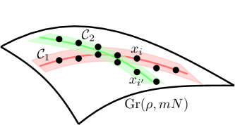
(a) Clusters on $\text{Gr}(\rho,mN)$

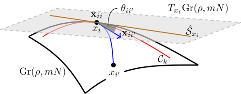
(b) Angular information

Figure 2: (a) The Riemannian multi-manifold modeling (RMMM) hypothesis. (b) Angular information computed in tangent spaces and used in Alg. 2.

1

Input : Grassmannian features $\{x_{i}\}_{i\in\mathfrak{I}}$.

2

Parameters : $K_{\text{NN}}\in\mathbb{Z}_{>0}$ and $\sigma_{\alpha},\sigma_{\theta}\in\mathbb{R}_{>0}$.

3

Output : Clusters $\{\mathcal{C}_{k}\}_{k=1}^{K}$.

4

5for all $i\in\mathfrak{I}$ do

6      

7      Define the $K_{\text{NN}}$-nearest-neighbors $\mathscr{N}_{\text{NN}}(x_{i})$.

8      Map $\mathscr{N}_{\text{NN}}(x_{i})$ into the tangent space $T_{x_{i}}\text{Gr}(\rho,mN)$ of the Grassmannian at $x_{i}$ via the logarithm map: $\mathbf{x}_{ii^{\prime}}\coloneqq\log_{x_{i}}(x_{i^{\prime}})$, $\forall x_{i^{\prime}}\in\mathscr{N}_{\text{NN}}(x_{i})$.

9      Identify $\{\alpha_{ii^{\prime}}\}_{x_{i^{\prime}}\in\mathscr{N}_{\text{NN}}(x_{i})}$ via (6). Set $\alpha_{ii^{\prime}}\coloneqq 0$, for all $i^{\prime}$ s.t. $x_{i^{\prime}}\notin\mathscr{N}_{\text{NN}}(x_{i})$.

10      Compute the sample correlation matrix $\hat{\mathbf{C}}_{x_{i}}$ in (7).

11      Perform principal component analysis (PCA) on $\hat{\mathbf{C}}_{x_{i}}$ to extract the eigenspace $\hat{\mathcal{S}}_{x_{i}}$.

12      Compute angle $\theta_{ii^{\prime}}$ between vector $\mathbf{x}_{ii^{\prime}}-\mathbf{x}_{ii}$ and $\hat{\mathcal{S}}_{x_{i}}$, $\forall x_{i^{\prime}}\in\mathscr{N}_{\text{NN}}(x_{i})$ (${\theta_{ii}}\coloneqq 0$). Let also $\theta_{ii^{\prime}}\coloneqq 0$ for $x_{i^{\prime}}\notin\mathscr{N}_{\text{NN}}(x_{i})$.

13

14Form the symmetric $\lvert\mathfrak{I}\rvert\times\lvert\mathfrak{I}\rvert$ affinity (adjacency) matrix $\mathbf{W}\coloneqq[w_{ii^{\prime}}]_{(i,i^{\prime})\in\mathfrak{I}^{2}}$, where entry $w_{ii^{\prime}}$ is defined as

$$w_{ii^{\prime}}\coloneqq\exp(\lvert\alpha_{ii^{\prime}}\rvert+\lvert\alpha_{i^{\prime}i}\rvert)\cdot\exp[-(\theta_{ii^{\prime}}+\theta_{i^{\prime}i})/\sigma_{\theta}]\,.$$

15Apply Louvain method [57] to $\mathbf{W}$ to map the data $(x_{i})_{i\in\mathfrak{I}}$ to clusters $\{\mathcal{C}_{k}\}_{k=1}^{K}$.

Algorithm 2 Geodesic clustering by tangent spaces (GCT)

A short description of the steps in Alg. 2 follows, with Riemannian-geometry details deferred to [45, 44, 43]. Alg. 2 visits $\{x_{i}\}_{i\in\mathfrak{I}}$ sequentially (step 2). At step 2, the $K_{\text{NN}}$-nearest-neighbors $\mathscr{N}_{\text{NN}}(x_{i})$ of $x_{i}$ are identified, i.e., those $K_{\text{NN}}$ points, taken from $\{x_{i}\}_{i}$, which are placed the closest from $x_{i}$ with respect to the Grassmannian distance [58]. The neighbors $\mathscr{N}_{\text{NN}}(x_{i})$ are then mapped at step 2 to the Euclidean vectors $\{\mathbf{x}_{ii^{\prime}}\}_{x_{i^{\prime}}\in\mathscr{N}_{\text{NN}}(x_{i})}$ in the tangent space $T_{x_{i}}\text{Gr}(\rho,mN)$ of the Grassmannian at $x_{i}$ (the gray-colored plane in Fig. 2b) via the logarithm map $\log_{x_{i}}(\cdot)$, whose computation (non-closed form via SVD) is provided in [45, 43]. Step 2 computes the weights $\{\alpha_{ii^{\prime}}\}_{x_{i^{\prime}}\in\mathscr{N}_{\text{NN}}(x_{i})}$, with $\alpha_{ii}\coloneqq 0$, via the following sparse-coding task:

$$\min_{\{\alpha_{ii^{\prime}}\}}{} {}\left\lVert\mathbf{x}_{ii}-\sum\nolimits_{x_{i^{\prime}}\in\mathscr{N}_{\text{NN}}(x_{i})\setminus\{x_{i}\}}\alpha_{ii^{\prime}}\mathbf{x}_{ii^{\prime}}\right\rVert^{2}$$

$${}+\sum\nolimits_{x_{i^{\prime}}\in\mathscr{N}_{\text{NN}}(x_{i})\setminus\{x_{i}\}}\exp[{\lVert\mathbf{x}_{ii^{\prime}}-\mathbf{x}_{ii}\rVert/\sigma_{\alpha}}]\cdot|\alpha_{ii^{\prime}}|$$

s.to $${}\sum\nolimits_{x_{i^{\prime}}\in\mathscr{N}_{\text{NN}}(x_{i})\setminus\{x_{i}\}}\alpha_{ii^{\prime}}=1\,.$$ (6)

The affine constraint in (6), imposed on the $\{\alpha_{ii^{\prime}}\}$ coefficients in representing $\mathbf{x}_{ii}$ via its neighbors, is motivated by the affine nature of the tangent space (Fig. 2b). Moreover, the larger the distance of neighbor $\mathbf{x}_{ii^{\prime}}$ from $\mathbf{x}_{ii}$, the larger the weight $\exp[{\lVert\mathbf{x}_{ii^{\prime}}-\mathbf{x}_{ii}\rVert/\sigma_{\alpha}}]$, which in turn penalizes severely the coefficient $\alpha_{ii^{\prime}}$ by pushing it to values close to zero. Step 2 computes the sample covariance matrix

$$\hat{\mathbf{C}}_{x_{i}}\coloneqq\tfrac{1}{\lvert\mathscr{N}_{\text{NN}}(x_{i})\rvert-1}\sum\nolimits_{x_{i^{\prime}}\in\mathscr{N}_{\text{NN}}(x_{i})}(\mathbf{x}_{ii^{\prime}}-\bar{\mathbf{x}}_{i})(\mathbf{x}_{ii^{\prime}}-\bar{\mathbf{x}}_{i})^{\intercal}\,,$$ (7)

where $\bar{\mathbf{x}}_{i}\coloneqq(1/\lvert\mathscr{N}_{\text{NN}}(x_{i})\rvert)\sum_{x_{i^{\prime}}\in\mathscr{N}_{\text{NN}}(x_{i})}\mathbf{x}_{ii^{\prime}}$ denotes the sample average of the neighbors of $\mathbf{x}_{ii}$. PCA is applied to $\hat{\mathbf{C}}_{x_{i}}$ at step 2 to compute the principal eigenspace $\hat{S}_{x_{i}}$, which may be viewed as an approximation of the image of the cluster (submanifold) $\mathcal{C}_{k}$, via the logarithm map, into the tangent space $T_{x_{i}}\text{Gr}(\rho,mN)$ (see Fig. 2b). Once $\hat{S}_{x_{i}}$ is computed, the angle $\theta_{ii^{\prime}}$ between vector $\mathbf{x}_{ii^{\prime}}-\mathbf{x}_{ii}$ and $\hat{\mathcal{S}}_{x_{i}}$ is also computed at step 2 to extract angular information. The larger the angle $\theta_{ii^{\prime}}$ is, the less the likelihood for $x_{i^{\prime}}$ to belong to cluster $\mathcal{C}_{k}$. The information carried by both $\{\alpha_{ii^{\prime}}\}$ and the angles $\{\theta_{ii^{\prime}}\}$ is used to define the adjacency matrix $\mathbf{W}$ at step 2. The use of angular information here, as well as in [45, 44, 43], advances the boundary of state-of-the-art clustering methods in the Grassmannian, where usually the weights of the adjacency matrix are defined via the Grassmannian (geodesic) distance or sparse-coding schemes [56].

1

Input : Time series $\{(\prescript{}{\nu}{y}_{t})_{t\in\mathbb{Z}}\}_{\nu\in\mathcal{N}}$.

2

Output : Clusters $\{\mathcal{C}_{k}\}_{k=1}^{K}$.

3

4

5

6Function MainModule($\{(\prescript{}{\mathcal{V}}{\mathbf{y}}_{t})_{t\in\mathfrak{T}}\}_{\mathcal{V}\in\mathfrak{N}}$) :

7       Apply Alg. 1 to obtain features $\{x_{i}\}_{i\in\mathfrak{I}}$.

8      Apply Alg. 2 to map $\{x_{i}\}_{i\in\mathfrak{I}}$ to clusters $\{\mathcal{C}_{k}\}_{k=1}^{K}$.

9      return $\{\mathcal{C}_{k}\}_{k=1}^{K}$.

10

11if “state clustering” then

12      

13      Set $(\mathcal{V},\mathfrak{N})\coloneqq(\mathcal{N},\{\mathcal{N}\})$ and form data $(\prescript{}{\mathcal{N}}{\mathbf{y}}_{t})_{t\in\mathfrak{T}}$ according to Sec. II-A.

14      Call MainModule($(\prescript{}{\mathcal{N}}{\mathbf{y}}_{t})_{t\in\mathfrak{T}}$) to identify clusters/states.

15 else if “community detection”  then

16      

17      Set $(\mathcal{V},\mathfrak{N})\coloneqq(\mathcal{N},\{\mathcal{N}\})$ and form data $(\prescript{}{\mathcal{N}}{\mathbf{y}}_{t})_{t\in\mathfrak{T}}$ according to Sec. II-A.

18      Call MainModule($(\prescript{}{\mathcal{N}}{\mathbf{y}}_{t})_{t\in\mathfrak{T}}$) to identify states, i.e., cluster the time horizon $\mathfrak{T}$ into a partition $\{\mathfrak{T}_{j}\}_{j=1}^{J}$ s.t. data $\{(\prescript{}{\nu}{y}_{t})_{t\in\mathfrak{T}_{j}}\}_{\nu\in\mathcal{N}}$ belong to the same state.

19      for $j=1$ to $J$ do

20            

21            Set $(\mathcal{V},\mathfrak{N})\coloneqq(\nu,\mathcal{N})$ and form data $\{(\prescript{}{\nu}{\mathbf{y}}_{t})_{t\in\mathfrak{T}_{j}}\}_{\nu\in\mathcal{N}}$ according to Sec. II-B.

22            Call MainModule($\{(\prescript{}{\nu}{\mathbf{y}}_{t})_{t\in\mathfrak{T}_{j}}\}_{\nu\in\mathcal{N}}$) to identify communities in state $j$.

23      

24 else if “subnetwork-state-sequence clustering” then

25      

26      Call lines 3 and 3 to identify states, i.e., a partition $\{\mathfrak{T}_{j}\}_{j=1}^{J}$ of $\mathfrak{T}$.

27      for $j=1$ to $J$ do

28            

29            Set $(\mathcal{V},\mathfrak{N})\coloneqq(\nu,\mathcal{N})$ and form data $\{(\prescript{}{\nu}{\mathbf{y}}_{t})_{t\in\mathfrak{T}_{j}}\}_{\nu\in\mathcal{N}}$ according to Sec. II-B.

30            Apply Alg. 1 to $\{(\prescript{}{\nu}{\mathbf{y}}_{t})_{t\in\mathfrak{T}_{j}}\}_{\nu\in\mathcal{N}}$ to obtain the Grassmannian features $\{[\prescript{j}{\nu}{\hat{\mathbf{O}}}_{t}]\}_{t\in\mathfrak{T}_{j}}$.

31      

32      Form features $\{x_{i}\}_{i\in\mathfrak{I}}\coloneqq\cup_{j=1}^{J}\cup_{\nu\in\mathcal{N}}\cup_{t\in\mathfrak{T}_{j}}[\prescript{j}{\nu}{\hat{\mathbf{O}}}_{t}]$.

33      Apply Alg. 2 to $\{x_{i}\}_{i\in\mathfrak{I}}$ to identify clusters/tasks.

34

Algorithm 3 Clustering framework

To summarize, the clustering framework is presented in pseudo-code form in Alg. 3. More specifically, the main module of the framework, which is frequently utilized and contains Algs. 1 and 2, is presented at steps 3–3. While the “state-clustering” part (steps 3–3) is quite straightforward, the “community detection” (steps 3–3) and “subnetwork-state-sequence clustering” (steps 3–3) comprise several steps. More specifically, in “community detection” (steps 3–3), states are first identified via steps 3–3 and then communities are identified in steps 3–3 within each state. In “subnetwork-state-sequence clustering” (steps 3–3), states are again identified first in step 3, the Grassmannian features are extracted in steps 3–3, all features are gathered as $\{x_{i}\}_{i\in\mathfrak{I}}$ in step 3, and finally Alg. 2 is applied to $\{x_{i}\}_{i\in\mathfrak{I}}$ to identify clusters/tasks in step 3.

To achieve a high accuracy clustering result, it is necessary to cluster states first, before applying community detection and subnetwork-state-sequence clustering. Without knowing the starting and ending points of different states, there will be time-series vectors $\prescript{}{\nu}{\mathbf{y}}_{t}$ in Alg. 1 which capture data from two consecutive states, since $\prescript{}{\nu}{\mathbf{y}}_{t}$ takes the form of $[\prescript{}{\nu}{y}_{t},\ldots,\prescript{}{\nu}{y}_{t+\texttt{Buff}_{\nu}-1}]^{\intercal}$. Features corresponding to those vectors will decrease the clustering accuracy since the extracted features do not correspond to any actual state or task.

The main computational burden comes from the module of steps 3–3 in Alg. 3. If $\mathfrak{I}_{\mathcal{V}}$ denotes the points in the Grassmannian, the computational complexity for computing features $\{x_{i}\}_{i\in\mathfrak{I}_{\mathcal{V}}}$ in Alg. 1 is $\mathcal{O}(|\mathfrak{I}_{\mathcal{V}}|\mathcal{C}_{\operatorname{\otimes_{\mathcal{H}}}})$, where $\mathcal{C}_{\operatorname{\otimes_{\mathcal{H}}}}$ denotes the cost of computing $\bm{\mathcal{F}}_{t+1}\operatorname{\otimes_{\mathcal{H}}}\bm{\mathcal{B}}_{t}^{\intercal}$, which includes SVD computations. In Alg. 2, the complexity for computing the $\mathscr{N}_{\text{NN}}(x_{i})$ nearest neighbors of $x_{i}$ is $\mathcal{O}(|\mathfrak{I}_{\mathcal{V}}|\mathcal{C}_{\text{dist}}+\mathscr{N}_{\text{NN}}\log|\mathfrak{I}_{\mathcal{V}}|)$, where $\mathcal{C}_{\text{dist}}$ denotes the cost of computing the Riemannian distance between any two points, and $\mathscr{N}_{\text{NN}}\log|\mathfrak{I}_{\mathcal{V}}|$ refers to the cost of finding the $\mathscr{N}_{\text{NN}}$ nearest neighbors of $x_{i}$. Step 2 of Alg. 2 is a sparsity-promoting optimization task of (6) and let $\mathcal{C}_{\text{SC}}$ denotes the complexity to solve it. Under $\mathcal{M}\coloneqq\text{Gr}(\rho,mN)$, step 2 of Alg. 2 involves the computation of the eigenvectors of the sample covariance matrix $\hat{\mathbf{C}}_{x_{i}}$, with complexity of $\mathcal{O}(\dim\mathcal{M}+K_{\text{NN}}^{3})$. In step 2, the complexity for computing empirical geodesic angles is $\mathcal{O}[|\mathfrak{I}_{\mathcal{V}}|(\mathcal{C}_{\log}+\dim\mathcal{M})]$, where $\mathcal{C}_{\log}$ is the complexity of computing the logarithm map $\log_{x_{i}}(\cdot)$ [43]. For the last step of Alg. 2, the exact complexity of Louvain method is not known but the method seems to run in time $\mathcal{O}(|\mathfrak{I}_{\mathcal{V}}|\log|\mathfrak{I}_{\mathcal{V}}|)$ with most of the computational effort spent on modularity optimization at first level, since modularity optimization is known to be NP-hard [59]. To summarize, the complexity of Alg. 2 is $\mathcal{O}[|\mathfrak{I}_{\mathcal{V}}|^{2}(\mathcal{C}_{\text{dist}}+\mathcal{C}_{\log}+\dim\mathcal{M})+(K_{\text{NN}}+1)|\mathfrak{I}_{\mathcal{V}}|\log|\mathfrak{I}_{\mathcal{V}}|+|\mathfrak{I}_{\mathcal{V}}|(\dim\mathcal{M}+K_{\text{NN}}^{3})]$.

IV Numerical Tests

This section validates the proposed framework on synthetic and real data. First, the competing clustering algorithms are briefly described.

IV-A Competing Algorithms

IV-A1 Sparse Manifold Clustering and Embedding (SMCE) [56]

Each point on the Grassmannian is described by a sparse affine combination of its neighbors. The computed sparse weights define the entries of a similarity matrix, which is subsequently used to identify data-cluster associations. SMCE does not utilize any angular information, as step 2 of Alg. 2 does.

IV-A2 Interaction K-means with PCA (IKM-PCA) [60]

IKM is a clustering algorithm based on the classical K-means and Euclidean distances within a properly chosen feature space. To promote time-efficient solutions, the classical PCA is employed as a dimensionality-reduction tool for feature-subset selection.

IV-A3 Graph-shift-operator estimation (GOE) [33]

The graph shift operator is a symmetric matrix capturing the network’s structure, i.e., topology. There are widely adopted choices of graph shift operators, including the adjacency and Laplacian matrices, or their various degree-normalized counterparts. An estimation algorithm in [33] computes the optimal graph shift operator via convex optimization. The computed graph shift operator is fed to a spectral-clustering module to identify communities within a single brain state, since [33] assumes stationary time-series data.

IV-A4 3D-Windowed Tensor Approach (3D-WTA) [38]

3D-WTA was originally introduced for community detection in dynamic networks by applying tensor decompositions onto a sequence of adjacency matrices indexed over the time axis. 3D-WTA was modified in [39] to accommodate multi-layer network structures. High-order SVD (HOSVD) and high-order orthogonal iteration (HOOI) are used within a pre-defined sliding window to extract subspace information from the adjacency matrices. The “asymptotic-surprise” metric is used as the criterion to determine the number of clusters. 3D-WTA is capable of performing both state clustering and community detection.

SMCE, 3D-WTA and the classical K-means will be compared against Alg. 3 on state clustering. SMCE, IKM-PCA, 3D-WTA, GOA and K-means will be used in community detection. Since none of IKM-PCA, GOA and 3D-WTA can perform subnetwork-state-sequence clustering across multiple states, only the results of Alg. 3 and SMCE are reported. To ensure fair comparisons, the parameters of all methods were carefully tuned to reach optimal performance for every scenario at hand.

In the following discussion, tags K-ARMA[S] and K-ARMA[M] denote the proposed framework whenever a single and multiple kernel functions are employed, respectively. In the case where the linear kernel is used, the K-ARMA method boils down to the ARMA method of [43].

The evaluation of all methods was based on the following three criteria: 1) Clustering accuracy, defined as the number of correctly clustered data points (ground-truth labels are known) over the total number of points; 2) normalized mutual information (NMI) [61]; and 3) the classical confusion matrix [62], with true-positive ratio (TPR), false-positive ratio (FPR), true-negative ratio (TNR), and false-negative ratio (FNR), in the case where the number of clusters to be identified is equal to two. In what follows, every numerical value of the previous criteria is the uniform average of $20$ independently performed tests for the particular scenario at hand.

IV-B Synthetic Data

IV-B1 fMRI Data

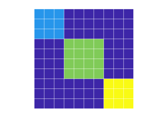
(a) State 1

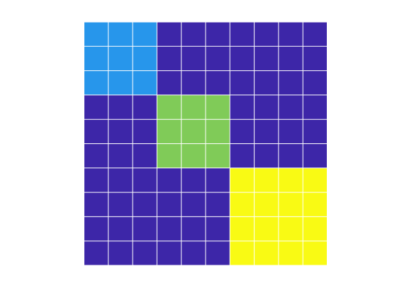
(b) State 2

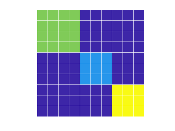
(c) State 3

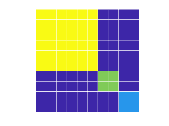
(d) State 4

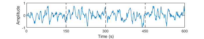
(e) BOLD time series of node #2, dataset #5

Figure 3: Synthetic data generated by the Matlab SimTB toolbox [12]. (a)-(d) Noiseless and outlier-free connectivity matrices corresponding to four network states. Nodes that share the same color cooperate to perform a common subnetwork task.

Data were generated by the open-source Matlab SimTB toolbox [12]. A $10$-node network is considered that transitions successively between $4$ distinct network states. Each state corresponds to a certain connectivity matrix, generated via the following path. Each connectivity matrix, fed to the SimTB toolbox, is modeled as the superposition of three matrices: 1) The ground-truth (noiseless) connectivity matrix (cf. Fig. 3), where nodes sharing the same color belong to the same cluster and collaborate to perform a common subnetwork task; 2) a symmetric matrix whose entries are drawn independently from a zero-mean Gaussian distribution with standard deviation $\sigma$ to model noise; and 3) a symmetric outlier matrix where $36$ entries are equal to $\mu$ to account for outlier neural activity.

Different states may share different outlier matrices, controlled by $\mu$. Aiming at extensive numerical tests, six datasets were generated (corresponding to the columns of Table I) by choosing six pairs of parameters $(\mu,\sigma)$ in the modeling of the connectivity matrices and the SimTB toolbox. Datasets 1, 2 and 3 (D1, D2 and D3) were created without outliers, while datasets 4, 5 and 6 (D4, D5 and D6) include outlier matrices with different $\mu$s in different states. Table IV details the parameters of those six datasets. Driven by the previous connectivity matrices, the SimTB toolbox generates BOLD time series [5]. Each state contributes $150$ signal samples, for a total of $4\times 150=600$ samples, to every nodal time series, e.g., Fig. 3e.

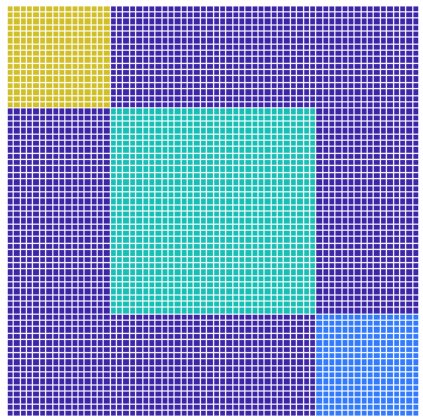
(a) State 1

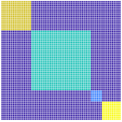
(b) State 2

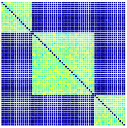
(c) D1S1

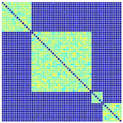
(d) D1S2

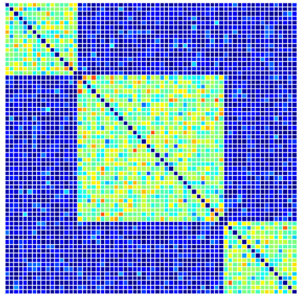
(e) D2S1

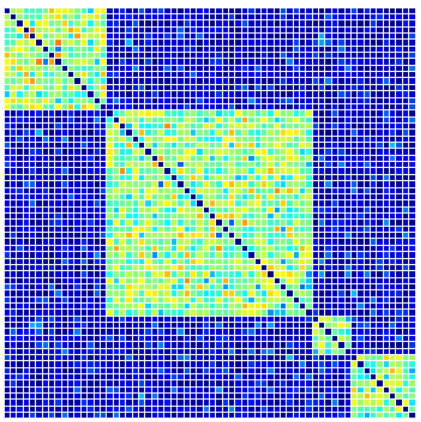
(f) D2S2

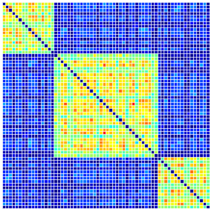
(g) D3S1

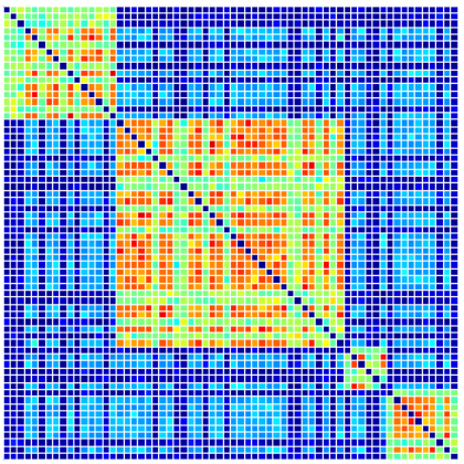
(h) D3S2

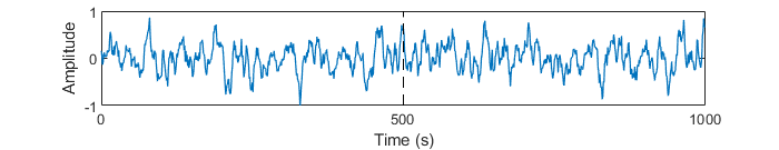
(i) EEG time series of node #27, dataset #2

Figure 4: Synthetic data generated by the Virtual Brain toolbox [63]. (a) and (b) Task connectivity matrices without noise for each state. There are three communities/tasks for state 1 and four tasks in state 2. (c)-(h) are connectivity matrices for each state of three datasets. (g) is the time series of 27th node of dataset 2.

Methods	Without Outliers						With Outliers
	Clustering Accuracy			NMI			Clustering Accuracy			NMI
	D1	D2	D3	D1	D2	D3	D4	D5	D6	D4	D5	D6
ARMA	0.969	0.805	0.640	0.948	0.766	0.596	0.944	0.743	0.589	0.860	0.627	0.340
K-ARMA[S]	1	0.824	0.671	1	0.791	0.622	0.983	0.775	0.599	0.930	0.651	0.379
K-ARMA[M]	1	0.839	0.708	1	0.808	0.641	0.992	0.800	0.626	0.967	0.689	0.435
3DWTA	1	0.792	0.603	1	0.735	0.556	0.943	0.721	0.517	0.872	0.558	0.281
SMCE	0.920	0.784	0.583	0.887	0.673	0.480	0.883	0.712	0.508	0.713	0.562	0.246
Kmeans	0.866	0.670	0.402	0.800	0.590	0.307	0.768	0.621	0.337	0.476	0.403	0.168

TABLE I: Synthetic fMRI Data: State clustering

Table I demonstrates the results of state clustering. The parameters used for ARMA and K-ARMA are: $N\coloneqq 30$, $m\coloneqq 2$, $\rho\coloneqq 2$, $\tau_{f}\coloneqq 60$, $\tau_{b}\coloneqq 20$. The Gaussian kernel $\kappa_{\text{G};0.8}(\cdot,\cdot)$ (cf. App. A) is used in the single-kernel method K-ARMA[S], while kernel $\kappa(\cdot,\cdot)\coloneqq 0.6\,\kappa_{\text{G};0.8}(\cdot,\cdot)+0.4\,\kappa_{\text{L};1}(\cdot,\cdot)$ is used in the K-ARMA[M] case since it performed the best among other choices of kernel functions. Fig. 5 depicts also the standard deviations of the results of Table I, computed after performing independent repetitions of the same test. Standard deviation of all algorithms increase when the strength of the noisy matrix increases. For dataset D1, K-ARMA[S], K-ARMA[M] and 3DWTA reach $100\%$ accuracy; for other datasets, K-ARMA[M] exhibits the highest accuracy and the smallest standard deviation.

3DWTA, K-ARMA[S] and K-ARMA[M] achieved perfect score ($100\%$) for both the clustering-accuracy and NMI metrics on dataset $1$. Among all methods, K-ARMA[M] scores the highest clustering accuracy and NMI over all six datasets. It can be observed by Table I that the existence of outliers affects negatively the ability of all methods to cluster data. The main reason is that the algorithms tend to detect outliers and gather those in clusters different from the nominal ones. Ways to reject those outliers are outside of the scope of this study and will be provided in a future publication.

Methods	Without Outliers						With Outliers
	Clustering Accuracy			NMI			Clustering Accuracy			NMI
	D1	D2	D3	D1	D2	D3	D4	D5	D6	D4	D5	D6
ARMA	1	0.960	0.842	1	0.876	0.775	0.973	0.910	0.817	0.940	0.793	0.664
K-ARMA[S]	1	1	0.915	1	1	0.838	1	0.942	0.852	1	0.864	0.710
K-ARMA[M]	1	1	0.945	1	1	0.907	1	0.958	0.879	1	0.892	0.803
3DWTA	1	0.941	0.839	1	0.927	0.754	0.925	0.863	0.799	0.842	0.780	0.638
SMCE	0.975	0.929	0.827	0.902	0.865	0.691	0.909	0.773	0.745	0.769	0.647	0.563
GOE	1	0.933	0.809	1	0.915	0.655	0.918	0.740	0.684	0.833	0.652	0.409
IKM-PCA	0.948	0.907	0.791	0.890	0.814	0.629	0.892	0.756	0.712	0.738	0.551	0.486
Kmeans	0.908	0.876	0.725	0.810	0.729	0.547	0.843	0.672	0.605	0.620	0.391	0.314

TABLE II: Synthetic fMRI data: Community detection

Table II presents the results of community detection. The numerical values in Table II stand for the average values over the $4$ states for each one of the datasets. Parameters of ARMA and K-ARMA were set as follows: $N\coloneqq 30$, $\texttt{Buff}_{\nu}\coloneqq 20$, $m\coloneqq 3$, $\rho\coloneqq 2$, $\tau_{f}\coloneqq 50$, $\tau_{b}\coloneqq 10$. In K-ARMA[S], the utilized kernel function is $\kappa_{\text{G};0.5}(\cdot,\cdot)$, while in K-ARMA[M] the kernel is defined as $\kappa(\cdot,\cdot)\coloneqq 0.5\,\kappa_{\text{G};0.5}(\cdot,\cdot)+0.5\,\kappa_{\text{L}0;1}(\cdot,\cdot)$ (cf. App. A). Table II demonstrates that K-ARMA[M] consistently outperforms all other methods across all datasets and even for the case where outliers contaminate the data. Fig. 6 depicts also the standard deviations of the results of Table II. ARMA, K-ARMA[S], K-ARMA[M] and 3DWTA score $100\%$ accuracy for dataset D1, while K-ARMA[S] and K-ARMA[M] show $100\%$ accuracy for dataset D4. K-ARMA[M] shows the highest accuracy on all other datasets.

Methods	Without Outliers						With Outliers
	Clustering Accuracy			NMI			Clustering Accuracy			NMI
	D1	D2	D3	D1	D2	D3	D4	D5	D6	D4	D5	D6
ARMA	1	0.816	0.749	1	0.767	0.684	0.928	0.701	0.633	0.874	0.484	0.355
K-ARMA[S]	1	0.856	0.781	1	0.791	0.702	0.956	0.728	0.664	0.913	0.534	0.410
K-ARMA[M]	1	0.884	0.817	1	0.821	0.739	1	0.757	0.721	1	0.602	0.485
SMCE	0.936	0.792	0.691	0.804	0.617	0.495	0.851	0.665	0.580	0.785	0.416	0.318

TABLE III: Synthetic fMRI data: Subnetwork state sequences

Table III illustrates the results of task clustering on $4$ synthetic-fMRI datasets: D1, D2, D3, D4, D5 and D6. The parameters of ARMA and Kernel ARMA were set as follows: $N\coloneqq 20$, $\texttt{Buff}_{\nu}\coloneqq 50$, $m\coloneqq 3$, $\rho\coloneqq 3$, $\tau_{f}\coloneqq 45$, $\tau_{b}\coloneqq 5$. The kernel functions used in K-ARMA[S] and K-ARMA[M] are identical to those employed in Table II. Similarly to the previous cases, K-ARMA[M] outperforms all other methods across all datasets and scenarios on both clustering accuracy and NMI. Fig. 7 depicts also the standard deviations of the results of Table III. ARMA, K-ARMA[S] and K-ARMA[M] score $100\%$ accuracy on dataset D1. K-ARMA[M] shows the highest accuracy with the smallest standard deviation on all other datasets.

Table IV provides the parameters $\mu$ and $\sigma$ used to generate noise matrices and symmetric matrices to simulate outlier neural activities. By choosing different combinations of $(\mu,\sigma)$, $6$ different synthetic fMRI datasets were created.

TABLE IV: Parameters $(\mu,\sigma)$ used to generate synthetic BOLD time series

Dataset	State 1	State 2	State 3	State 4
1	$(0,-10\text{dB})$	$(0,-10\text{dB})$	$(0,-10\text{dB})$	$(0,-10\text{dB})$
2	$(0,-8\text{dB})$	$(0,-8\text{dB})$	$(0,-8\text{dB})$	$(0,-8\text{dB})$
3	$(0,-6\text{dB})$	$(0,-6\text{dB})$	$(0,-6\text{dB})$	$(0,-6\text{dB})$
4	$(0.2,-10\text{dB})$	$(0.3,-10\text{dB})$	$(0.4,-10\text{dB})$	$(0.5,-10\text{dB})$
5	$(0.2,-8\text{dB})$	$(0.3,-8\text{dB})$	$(0.4,-8\text{dB})$	$(0.5,-8\text{dB})$
6	$(0.2,-6\text{dB})$	$(0.3,-6\text{dB})$	$(0.4,-6\text{dB})$	$(0.5,-6\text{dB})$

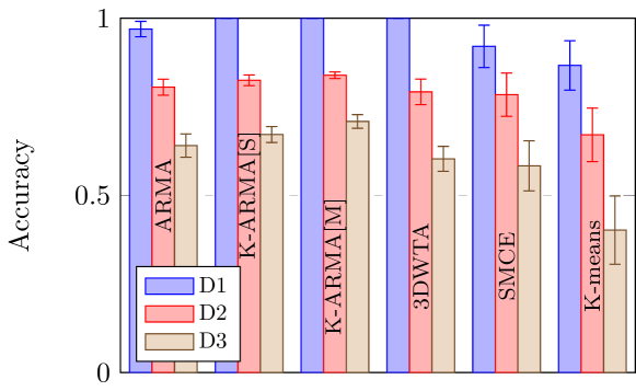
(a) Datasets 1, 2, 3

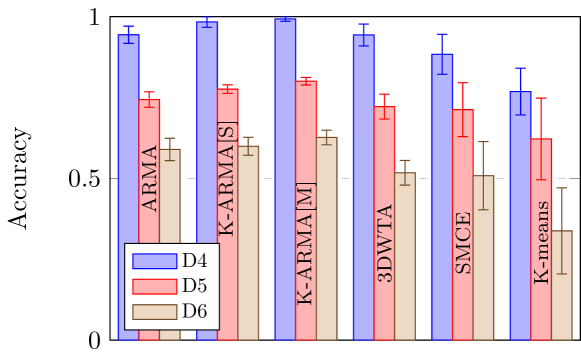
(b) Datasets 4, 5, 6

Figure 5: State-clustering results of synthetic fMRI datasets. (a) Data without an independent event; (b) Data with an independent event.

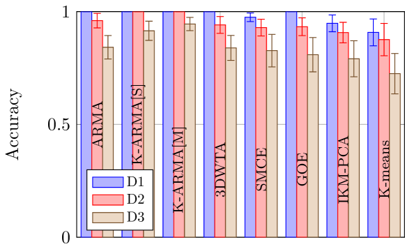
(a) Datasets 1, 2, 3

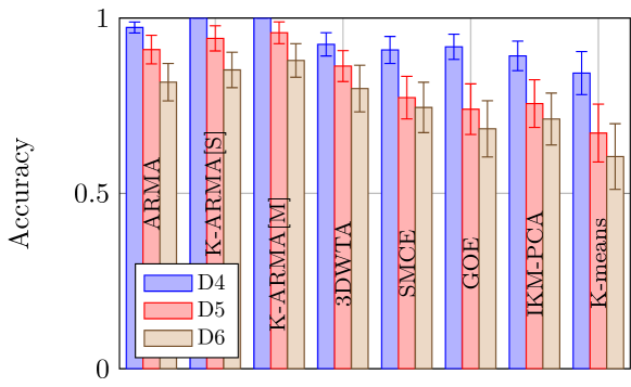
(b) Datasets 4, 5, 6

Figure 6: Community detection results of synthetic fMRI datasets. (a) Data without an independent event; (b) Data with an independent event.

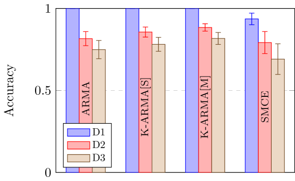
(a) Datasets 1, 2, 3

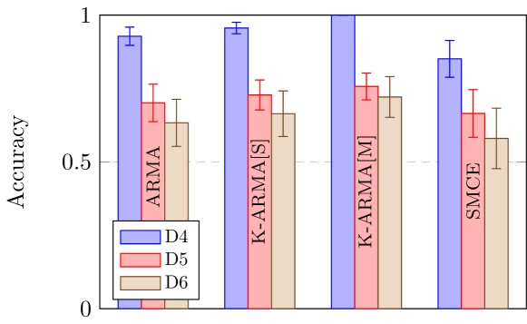
(b) Datasets 4, 5, 6

Figure 7: Subnetwork-state-sequence clustering results of synthetic fMRI datasets. (a) Data without an independent event; (b) Data with an independent event.

IV-B2 EEG Data

Synthetic EEG data were generated by the open-source Virtual Brain (VB) toolbox [63]. A $60$-node network is considered that transitions between two states, with noiseless and outlier-free connectivity matrices depicted in Figs. 4a and 4b. It is worth noticing that the number of communities in Fig. 4a is $3$, while $4$ in Fig. 4b. Similarly to the previous fMRI case, every connectivity matrix, which is fed to the VB toolbox [63], is the superposition of three matrices: The ground-truth matrix (cf. Figs. 4a and 4b), the “noise” and the “outlier” matrices. Three scenarios/datasets are considered, with the noisy and outlier-contaminated connectivity matrices illustrated in Figs. 4c–4h. Each state contributes $500$ signal samples, for a total of $2\times 500=1,000$ samples, to every nodal time series, e.g., Fig. 4i.

Methods	Clustering Accuracy			NMI
	D1	D2	D3	D1	D2	D3
ARMA	1	1	0.944	1	1	0.906
K-ARMA[S]	1	1	0.963	1	1	0.926
K-ARMA[M]	1	1	0.992	1	1	0.984
3DWTA	1	0.976	0.939	1	0.942	0.896
SMCE	0.952	0.901	0.804	0.914	0.852	0.766
Kmeans	0.879	0.793	0.732	0.796	0.761	0.694

TABLE V: Synthetic EEG data: State clustering

The results of state clustering are shown in Table V; standard deviations are also included in Fig. 8. Parameters of ARMA and K-ARMA were set as follows: $N\coloneqq 100$, $m\coloneqq 2$, $\rho\coloneqq 2$, $\tau_{f}\coloneqq 150$, $\tau_{b}\coloneqq 30$. The reproducing kernel used are $\kappa_{\text{G};0.5}(\cdot,\cdot)$ for K-ARMA[S], and $\kappa(\cdot,\cdot)\coloneqq 0.5\,\kappa_{\text{G};0.5}(\cdot,\cdot)+0.5\,\kappa_{\text{L};1}(\cdot,\cdot)$ for K-ARMA[M]. Furthermore, since clustering on dataset 3 is performed between two states, the entries of the confusion matrix for 3DWTA are $\text{TPR}=0.911$, $\text{FPR}=0.032$, $\text{FNR}=0.088$ and $\text{TNR}=0.967$, while those for K-ARMA[S] are $\text{TPR}=0.955$, $\text{FPR}=0.028$, $\text{FNR}=0.044$ and $\text{TNR}=0.971$. Fig. 8 depicts the standard deviations of the results of Table V. Due to noise and outliers, all algorithms show the highest accuracy on dataset 1 and the lowest accuracy on dataset 3. ARMA,K-ARMA[S], K-ARMA[M] and 3DWTA score $100\%$ accuracy on dataset 1. ARMA, K-ARMA[S], and K-ARMA[M] exhibit $100\%$ accuracy on dataset 2, while K-ARMA[M] scores the highest accuracy and the smallest standard deviation on all other datasets.

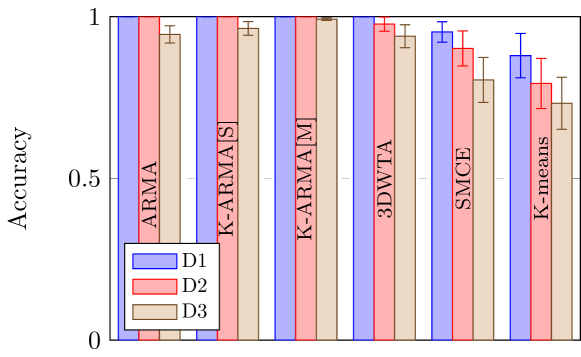
Figure 8: State-clustering results of synthetic EEG data.

Methods	Clustering accuracy			NMI
	D1	D2	D3	D1	D2	D3
ARMA	1	0.975	0.923	1	0.924	0.861
K-ARMA[S]	1	1	0.958	1	1	0.895
K-ARMA[M]	1	1	0.972	1	1	0.921
3DWTA	1	1	0.867	1	1	0.753
SMCE	1	0.951	0.833	1	0.887	0.706
GOE	1	0.946	0.785	1	0.869	0.684
IKM-PCA	0.961	0.913	0.811	0.935	0.847	0.652
Kmeans	0.894	0.808	0.696	0.836	0.713	0.530

TABLE VI: Synthetic EEG data: Community detection

Table VI illustrates the results of community detection of synthetic EEG datasets, which include three time series (D1–D3) across two states. The illustrated values are the average results over the two network states per time series. The parameters of ARMA, K-ARMA[S] and K-ARMA[M] were set as follows: $N\coloneqq 50$, $\texttt{Buff}_{\nu}=50$, $m\coloneqq 3$, $\rho\coloneqq 3$, $\tau_{f}\coloneqq 200$, $\tau_{b}\coloneqq 10$. Moreover, $\kappa_{\text{G};0.5}(\cdot,\cdot)$ was used as the reproducing kernel function in K-ARMA[S], while $\kappa(\mathbf{x},\mathbf{x}^{\prime})\coloneqq 0.5\,\kappa_{\text{G};0.5}(\mathbf{x},\mathbf{x}^{\prime})+0.5\,\kappa_{\text{L};0.8}(\mathbf{x},\mathbf{x}^{\prime})$ in K-ARMA[M]. Fig. 9 depicts also the standard deviations of the results of Table VI. Due to noise and outliers, all algorithms show their highest accuracies on dataset 1 and their lowest one on dataset 3. ARMA, K-ARMA[S], K-ARMA[M] and 3DWTA show $100\%$ accuracy on dataset 1. K-ARMA[S], K-ARMA[M] and 3DWTA score $100\%$ accuracy on dataset 2. K-ARMA[M] still shows the highest accuracy with the smallest standard deviation on all other datasets.

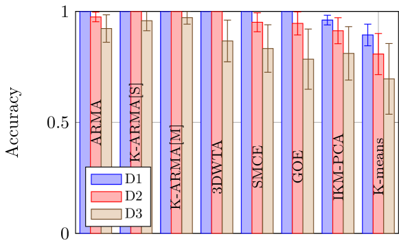
Figure 9: Community-detection results of synthetic EEG datasets.

Methods	Unknown state label						Known state label
	Clustering accuracy			NMI			Clustering accuracy			NMI
	D1	D2	D3	D1	D2	D3	D1	D2	D3	D1	D2	D3
ARMA	1	0.932	0.798	1	0.882	0.710	1	0.978	0.929	1	0.947	0.890
K-ARMA[S]	1	0.944	0.859	1	0.903	0.794	1	1	0.965	1	1	0.943
K-ARMA[M]	1	0.965	0.877	1	1	0.816	1	1	1	1	1	1
SMCE	0.975	0.902	0.755	0.931	0.857	0.629	1	0.940	0.886	1	0.899	0.828

TABLE VII: Synthetic EEG Data: Subnetwork state sequences

Results of subnetwork-state-sequence clustering for the EEG synthetic data are shown in Table VII. The utilized parameters and kernel functions were chosen to be the same as in the previous case of community detection. ARMA, K-ARMA[S] and K-ARMA[M] got 100% accuracy and NMI for dataset D1, since the standard deviation of “noise” matrices are small and dataset D1 does not include outliers. It can be clearly verified by Table VII that if the “true” state labels are known beforehand, and thus step 3 in Alg. 3 is not needed, then all values of clustering accuracies and NMI increase. Fig. 10 depicts also the standard deviations of the results of Table VII. By comparing the two figures in Fig. 10, it can be clearly seen that if the “true” state labels are known beforehand, i.e., step 3 in Alg. 3 is not needed, then all values of clustering accuracies increase while standard deviations decrease. Similarly to other tests, K-ARMA[M] shows the highest accuracy on all datasets.

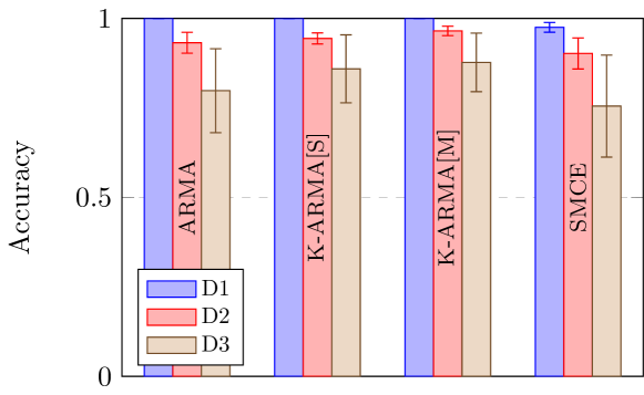
(a) Estimated state label

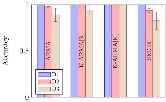
(b) True state label

Figure 10: Subnetwork-state-sequence clustering results of synthetic EEG datasets. (a) With estimated state label; (b) with true state label.

IV-C Real Data

The open-source real EEG data [64] were used. The data comprise five sets (A–E), each containing $100$ single-channel segments of $23.6$-sec duration. The sampling rate of the data was $173.61$ Hz. Only state clustering is examined, since data [64] do not contain any connectivity-structure information. Datasets D and E were chosen, where set D contains only activity measured during seizure free intervals, while set E contains only seizure activity. The length of the time series extracted from the data was set equal to $4,096$. Methods ARMA, K-ARMA[S], K-ARMA[M], SMCE and K-means were validated. 3D-WTA did not perform well on those datasets, and thus, its results are not shown here.

Toward a realistic scenario, the time series of the sets D and E are concatenated to create a single time series with length $2\cdot 4,096=8,192$. The network has 100 nodes, so $|\mathcal{N}|\coloneqq 100$. Parameters of ARMA, K-ARMA[S] and K-ARMA[M] are defined as: $N\coloneqq 200$, $m\coloneqq 3$, $\rho\coloneqq 2$, $\tau_{f}\coloneqq 1800$, $\tau_{b}\coloneqq 50$. In K-ARMA[S], the kernel function is set equal to $\kappa_{\text{G};0.6}(\cdot,\cdot)$, while in K-ARMA[M] $\kappa(\cdot,\cdot)\coloneqq 0.5\,\kappa_{\text{G};0.6}(\cdot,\cdot)+0.5\,\kappa_{\text{L};0.8}(\cdot,\cdot)$. Due to the sliding-window implementation in the proposed framework, there are cases where the sliding window captures samples from both the D and E time series. The features extracted from those cases are labeled as cluster $3$. Fig. 11 depicts also the standard deviations of the results of Table VIII. K-ARMA[M] scores the highest clustering-accuracy and NMI values with the smallest standard deviation. In the case where the time series D and E are not concatenated, the case of sliding windows capturing data from both clusters (states) is non-existent. In such a binary-decision case, the confusion-matrix results of ARMA, K-ARMA[S] and K-ARMA[M] are $\text{TPR}=1$, $\text{FPR}=0$, $\text{FNR}=0$ and $\text{TNR}=1$, while for SMCE, $\text{TPR}=0.952$, $\text{FPR}=0.060$, $\text{FNR}=0.048$ and $\text{TNR}=0.939$.

TABLE VIII: Real EEG data: State clustering

Methods	Clustering accuracy	NMI
ARMA	0.907	0.844
K-ARMA[S]	0.925	0.886
K-ARMA[M]	0.939	0.921
SMCE	0.873	0.815
Kmeans	0.829	0.741

Real fMRI behavioral data, acquired from the Stellar Chance 3T scanner (SC3T) at the University of Pennsylvania, were used to cluster different states. The time series in data are collected in two arms before and after an inhibitory sequence of transcranial magnetic stimulation (TMS) known as continuous theta burst stimulation [65]. Real and Sham stimulation of two different tasks were applied for TMS. The two behavioral tasks are: 1) Navon task: A big shape made up of little shapes is shown on the screen. The big shape can either be green or white in color. If green, participant identifies the big shape, while if white, the participant identifies the little shape. The task was presented in three blocks: All white stimuli, all green stimuli, and switching between colors on 70% of trials to introduce switching demands. Responses given via button box are in the order of circle, x, triangle, square; 2) Stroop task: Words are displayed in different color inks. There are two difficulty conditions; one where subjects respond to words that introduced low color-word conflict (far, deal, horse, plenty) or high conflict with color words differing from the color the word is printed in (e.g., red printed in blue, green printed in yellow, etc.) [66]. The participant has to tell the color of the ink the word is printed in using a button box in the order of red, green, yellow, blue.

Each BOLD time series was collected during an $8$min scan with $\text{TR}=500$ms, which means that the length of time series is $956$. The time series has $83$ cortical and subcortical regions so $|\mathcal{N}|\coloneqq 83$. To test the state clustering results of fMRI time series, 3 states are concatenated to create a single time series with length $3\times 956=2,868$. The 3 states are: 1) Before real stimulation of the Navon task; 2) after real stimulation of the Navon task; and 3) after real stimulation of the Stroop task.

Parameters of ARMA, K-ARMA[S] and K-ARMA[M] are defined as: $N\coloneqq 180$, $m\coloneqq 4$, $\rho\coloneqq 2$, $\tau_{f}\coloneqq 350$, $\tau_{b}\coloneqq 20$. In K-ARMA[S], the kernel function is set equal to $\kappa_{\text{G};0.45}(\cdot,\cdot)$, while in K-ARMA[M] $\kappa(\cdot,\cdot)\coloneqq 0.3\,\kappa_{\text{G};0.25}(\cdot,\cdot)+0.3\,\kappa_{\text{G};0.9}(\cdot,\cdot)+0.4\,\kappa_{\text{L};0.75}(\cdot,\cdot)$. Notice here that due to the sliding-window implementation in the proposed framework, there are cases where the sliding window captures samples from two consecutive states.

TABLE IX: Real fMRI data: State clustering results

Methods	Clustering accuracy	NMI
ARMA	0.885	0.809
K-ARMA[S]	0.904	0.843
K-ARMA[M]	0.919	0.875
SMCE	0.893	0.816
Kmeans	0.801	0.720

Results of state clustering on real fMRI data are revealed in Table IX. Fig. 12 depicts also the standard deviations of the results of Table IX. Again, K-ARMA[M] exhibits the highest clustering-accuracy and NMI values, with the smallest standard deviation among all employed methods.

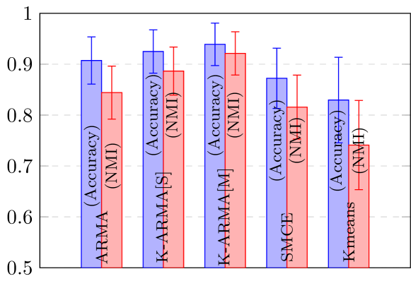
Figure 11: Real EEG data: State clustering.

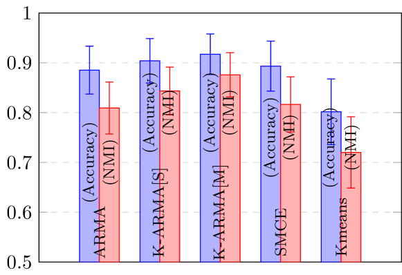
Figure 12: Real fMRI data: State clustering.

V Conclusions

This paper introduced a novel clustering framework to perform all possible clustering tasks in dynamic (brain) networks: state clustering, community detection and subnetwork-state-sequence tracking/identification. Features were extracted by a kernel-based ARMA model, with column spaces of observability matrices mapped to the Grassmann manifold (Grassmannian). A clustering algorithm, the geodesic clustering with tangent spaces, was also provided to exploit the rich underlying Riemannian geometry of the Grassmannian. The framework was validated on multiple simulated and real datasets and compared against state-of-the-art clustering algorithms. Test results demonstrate that the proposed framework outperforms the competing methods in clustering states, identifying community structures, and tracking multiple subnetwork state sequences which may span several network states. Current research effort includes finding ways to reduce the size of the computational footprint of the framework, and techniques to reject network-wide outlier data.

Appendix A Reproducing Kernel Hilbert Spaces

A reproducing kernel Hilbert space $\mathcal{H}$, equipped with inner product $\langle\cdot\mathop{}|\mathop{}\cdot\rangle_{\mathcal{H}}$, is a functional space where each point $g\in\mathcal{H}$ is a function $g:\mathbb{R}^{q}\to\mathbb{R}:\mathbf{y}\mapsto g(\mathbf{y})$, for some $q\in\mathbb{Z}_{>0}$, s.t. the mapping $g\mapsto g(\mathbf{y})$ is continuous, for any choice of $\mathbf{y}$ [67, 47, 68]. There exists a kernel function $\kappa(\cdot,\cdot):\mathbb{R}^{q}\times\mathbb{R}^{q}\to\mathbb{R}$, unique to $\mathcal{H}$, such that (s.t.) $\varphi(\mathbf{y})\coloneqq\kappa(\mathbf{y},\cdot)\in\mathcal{H}$ and $g(\mathbf{y})=\langle g\mathop{}|\mathop{}\varphi(\mathbf{y})\rangle_{\mathcal{H}}$, for any $g\in\mathcal{H}$ and any $\mathbf{y}\in\mathbb{R}^{q}$ [67, 68]. The latter property is the reason for calling kernel $\kappa$ reproducing, and yields the celebrated “kernel trick”: $\kappa(\mathbf{y}_{1},\mathbf{y}_{2})=\langle\kappa(\mathbf{y}_{1},\cdot)\mathop{}|\mathop{}\kappa(\mathbf{y}_{2},\cdot)\rangle_{\mathcal{H}}=\langle\varphi(\mathbf{y}_{1})\mathop{}|\mathop{}\varphi(\mathbf{y}_{2})\rangle_{\mathcal{H}}$, for any $\mathbf{y}_{1},\mathbf{y}_{2}\in\mathbb{R}^{q}$.

Popular examples of reproducing kernels are:

1. The linear $\kappa_{\text{lin}}(\mathbf{y}_{1},\mathbf{y}_{2})\coloneqq\mathbf{y}_{1}^{\intercal}\mathbf{y}_{2}$, where space $\mathcal{H}$ is nothing but $\mathbb{R}^{q}$;

2. the Gaussian $\kappa_{\text{G};\sigma}(\mathbf{y}_{1},\mathbf{y}_{2})\coloneqq\exp[-\lVert\mathbf{y}_{1}-\mathbf{y}_{2}\rVert^{2}/(2\sigma^{2})]$, where $\sigma\in\mathbb{R}_{>0}$ and $\lVert\cdot\rVert$ is the standard Euclidean norm. In this case, $\mathcal{H}$ is infinite dimensional [68];

3. the Laplacian $\kappa_{\text{L};\sigma}(\mathbf{y}_{1},\mathbf{y}_{2})\coloneqq\exp[-\lVert\mathbf{y}_{1}-\mathbf{y}_{2}\rVert_{1}/\sigma]$, where $\lVert\cdot\rVert_{1}$ stands for the $\ell_{1}$-norm [69]; and

4. the polynomial $\kappa_{\text{poly};r}(\mathbf{y}_{1},\mathbf{y}_{2})\coloneqq(\mathbf{y}_{1}^{\intercal}\mathbf{y}_{2}+1)^{r}$, for some parameter $r\in\mathbb{Z}_{>0}$.

There are several ways of generating reproducing kernels via certain operations on well-known kernel functions such as convex combinations, products, etc. [47].

Define $\mathcal{H}^{p}$, for some $p\in\mathbb{Z}_{>0}$, as the space whose points take the following form: $\bm{g}\coloneqq[g_{1},\ldots,g_{p}]^{\intercal}\in\mathcal{H}^{p}$ s.t. $g_{j}\in\mathcal{H}$, $\forall j\in\overline{1,p}$, where $\overline{1,p}$ is a compact notation for $\{1,\ldots,p\}$. For $p^{\prime}\in\mathbb{Z}_{>0}$ and given a matrix $\mathbf{A}\coloneqq[a_{ij}]\in\mathbb{R}^{p^{\prime}\times p}$, the product $\mathbf{A}\bm{g}\in\mathcal{H}^{p^{\prime}}$ stands for the vector-valued function whose $i$th entry is $\sum_{j=1}^{p}a_{ij}g_{j}$. Similarly, define $\mathcal{H}^{p_{1}\times p_{2}}$, for some $p_{1},p_{2}\in\mathbb{Z}_{>0}$, as the space comprising all

$$\bm{\mathcal{G}}\coloneqq\begin{bmatrix}g_{11}&\cdots&g_{1p_{2}}\\ \vdots&\ddots&\vdots\\ g_{p_{1}1}&\cdots&g_{p_{1}p_{2}}\end{bmatrix}\in\mathcal{H}^{p_{1}\times p_{2}}\,,$$

s.t. $g_{ij}\in\mathcal{H}$, $\forall i\in\overline{1,p_{1}}$, $\forall j\in\overline{1,p_{2}}$. Moreover, given $\bm{\mathcal{G}}\in\mathcal{H}^{p_{1}\times p}$ and $\bm{\mathcal{G}}^{\prime}\in\mathcal{H}^{p\times p_{2}}$, define the “product” $\bm{\mathcal{G}}\operatorname{\otimes_{\mathcal{H}}}\bm{\mathcal{G}}^{\prime}$ as the $p_{1}\times p_{2}$ matrix whose $(i,j)$th entry is

$$[\bm{\mathcal{G}}\operatorname{\otimes_{\mathcal{H}}}\bm{\mathcal{G}}^{\prime}]_{ij}\coloneqq\sum\nolimits_{l=1}^{p}\langle g_{il}\mathop{}|\mathop{}g_{lj}^{\prime}\rangle_{\mathcal{H}}\,.$$

In the case where $g_{il}\coloneqq\varphi(\mathbf{y}_{il})=\kappa(\mathbf{y}_{il},\cdot)$ and $g_{lj}^{\prime}\coloneqq\varphi(\mathbf{y}_{lj}^{\prime})=\kappa(\mathbf{y}_{lj}^{\prime},\cdot)$, for some $\mathbf{y}_{il},\mathbf{y}_{lj}^{\prime}$, as in (3), then the kernel trick suggests that the previous formula simplifies to $[\bm{\mathcal{G}}\operatorname{\otimes_{\mathcal{H}}}\bm{\mathcal{G}}^{\prime}]_{ij}=\sum_{l=1}^{p}\kappa(\mathbf{y}_{il},\mathbf{y}_{lj}^{\prime})$.

Appendix B Proof of Proposition 1

By considering a probability space $(\Omega,\Sigma,\operatorname{\mathbb{P}})$, a basis $\{e_{n}\}_{n\in\mathbb{Z}_{>0}}$ of $\mathcal{H}$, and by omitting most of the entailing measure-theoretic details, the expectation of $g=\sum_{n\in\mathbb{Z}_{>0}}\gamma_{n}e_{n}\in\mathcal{H}$, where $\{\gamma_{n}\}_{n\in\mathbb{Z}_{>0}}$ are real-valued RVs, is defined as $\operatorname{\mathbb{E}}(g)\coloneqq\sum_{n\in\mathbb{Z}_{>0}}\operatorname{\mathbb{E}}(\gamma_{n})e_{n}$, provided that the latter sum converges in $\mathcal{H}$. Conditional expectations are similarly defined. All of the expectations appearing in this manuscript are assumed to exist. Due to the linearity of the inner product $\langle\cdot\mathop{}|\mathop{}\cdot\rangle_{\mathcal{H}}$, it can be verified that the conditional expectation $\operatorname{\mathbb{E}}\{\langle g\mathop{}|\mathop{}g^{\prime}\rangle_{\mathcal{H}}{\mathbin{}\mid\mathbin{}}g^{\prime}\}=\operatorname{\mathbb{E}}\{\sum_{n,n^{\prime}}\gamma_{n}\gamma_{n^{\prime}}\langle e_{n}\mathop{}|\mathop{}e_{n^{\prime}}\rangle_{\mathcal{H}}{\mathbin{}\mid\mathbin{}}g^{\prime}\}=\sum_{n^{\prime}}\gamma_{n^{\prime}}\sum_{n}\operatorname{\mathbb{E}}\{\gamma_{n}{\mathbin{}\mid\mathbin{}}g^{\prime}\}\langle e_{n}\mathop{}|\mathop{}e_{n^{\prime}}\rangle_{\mathcal{H}}=\langle\sum_{n}\operatorname{\mathbb{E}}\{\gamma_{n}{\mathbin{}\mid\mathbin{}}g^{\prime}\}e_{n}\mathop{}|\mathop{}\sum_{n^{\prime}}\gamma_{n^{\prime}}e_{n^{\prime}}\rangle_{\mathcal{H}}=\langle\operatorname{\mathbb{E}}\{g{\mathbin{}\mid\mathbin{}}g^{\prime}\}\mathop{}|\mathop{}g^{\prime}\rangle_{\mathcal{H}}$, and $\operatorname{\mathbb{E}}\{\langle g\mathop{}|\mathop{}g^{\prime}\rangle_{\mathcal{H}}\}=\langle\operatorname{\mathbb{E}}(g)\mathop{}|\mathop{}\operatorname{\mathbb{E}}(g^{\prime})\rangle_{\mathcal{H}}$ in the case where $g$ and $g^{\prime}$ are independent. It can be similarly verified that these properties, which hold for the inner product $\langle\cdot\mathop{}|\mathop{}\cdot\rangle$, are inherited by $\operatorname{\otimes_{\mathcal{H}}}$.

Induction on (1) suggests that $\forall\tau\in\mathbb{Z}_{\geq 0}$, $\bm{\varphi}_{t+\tau}=\mathbf{CA}^{\tau}\bm{\psi}_{t}+\sum_{k=1}^{\tau}\mathbf{CA}^{\tau-k}\bm{\omega}_{t+k}+\bm{\upsilon}_{t+\tau}$, where $\sum_{k=1}^{0}\mathbf{CA}^{-k}\bm{\omega}_{t+k}\coloneqq\mathbf{0}$. Then,

$$\bm{f}_{t} \coloneqq\left[\bm{\varphi}_{t}^{\intercal},\bm{\varphi}_{t+1}^{\intercal},\ldots,\bm{\varphi}_{t+m-1}^{\intercal}\right]^{\intercal}$$

$$=\mathbf{O}\bm{\psi}_{t}+\bm{e}_{t}\,,$$ (8)

where

$$\bm{e}_{t}\coloneqq\begin{bmatrix}\bm{\upsilon}_{t}\\ \mathbf{C}\bm{\omega}_{t+1}+\bm{\upsilon}_{t+1}\\ \sum_{k=1}^{2}\mathbf{CA}^{2-k}\bm{\omega}_{t+k}+\bm{\upsilon}_{t+2}\\ \vdots\\ \sum_{k=1}^{m-1}\mathbf{CA}^{m-1-k}\bm{\omega}_{t+k}+\bm{\upsilon}_{t+m-1}\end{bmatrix}\in\mathcal{H}^{mN}\,.$$

By observing that $\bm{\mathcal{F}}_{t}=[\bm{f}_{t},\bm{f}_{t+1},\ldots,\bm{f}_{t+\tau_{\text{f}}-1}]$, it can be verified that

$$\bm{\mathcal{F}}_{t}=\mathbf{O}\left[\bm{\psi}_{t},\bm{\psi}_{t+1},\ldots,\bm{\psi}_{t+\tau_{\text{f}}-1}\right]+\left[\bm{e}_{t},\bm{e}_{t+1},\ldots,\bm{e}_{t+\tau_{\text{f}}-1}\right]\,.$$

Moreover, notice that $\bm{\mathcal{B}}_{t}=[\bm{b}_{t},\bm{b}_{t+1},\ldots,\bm{b}_{t+\tau_{\text{f}}-1}]$, where

$$\bm{b}_{t}\coloneqq\left[\bm{\varphi}_{t}^{\intercal},\bm{\varphi}_{t-1}^{\intercal},\ldots,\bm{\varphi}_{t-\tau_{\text{b}}+1}^{\intercal}\right]^{\intercal}\in\mathcal{H}^{\tau_{\text{b}}N}\,.$$

Hence,

$$\tfrac{1}{\tau_{\text{f}}}\bm{\mathcal{F}}_{t+1}\operatorname{\otimes_{\mathcal{H}}}\bm{\mathcal{B}}_{t}^{\intercal}$$

$${}={} \tfrac{1}{\tau_{\text{f}}}\mathbf{O}\left[\bm{\psi}_{t+1},\ldots,\bm{\psi}_{t+\tau_{\text{f}}}\right]\operatorname{\otimes_{\mathcal{H}}}\bm{\mathcal{B}}_{t}^{\intercal}$$

$$+\tfrac{1}{\tau_{\text{f}}}\left[\bm{e}_{t+1},\ldots,\bm{e}_{t+\tau_{\text{f}}}\right]\operatorname{\otimes_{\mathcal{H}}}\bm{\mathcal{B}}_{t}^{\intercal}$$

$$= \mathbf{O}\,\tfrac{1}{\tau_{\text{f}}}\sum\nolimits_{l=1}^{\tau_{\text{f}}}\bm{\psi}_{t+l}\operatorname{\otimes_{\mathcal{H}}}\bm{b}_{t+l-1}^{\intercal}$$

$$+\tfrac{1}{\tau_{\text{f}}}\sum\nolimits_{l=1}^{\tau_{\text{f}}}\bm{e}_{t+l}\operatorname{\otimes_{\mathcal{H}}}\bm{b}_{t+l-1}^{\intercal}$$

$$= \mathbf{O}\,\tfrac{1}{\tau_{\text{f}}}\sum\nolimits_{l=1}^{\tau_{\text{f}}}\bm{\psi}_{t+l}\operatorname{\otimes_{\mathcal{H}}}[\bm{\psi}_{t+l-1}^{\intercal}\mathbf{C}^{\intercal},\ldots,\bm{\psi}_{t+l-\tau_{\text{b}}}^{\intercal}\mathbf{C}^{\intercal}]$$

$$+\mathbf{O}\,\tfrac{1}{\tau_{\text{f}}}\sum\nolimits_{l=1}^{\tau_{\text{f}}}\bm{\psi}_{t+l}\operatorname{\otimes_{\mathcal{H}}}[\bm{\upsilon}_{t+l-1}^{\intercal},\ldots,\bm{\upsilon}_{t+l-\tau_{\text{b}}}^{\intercal}]$$

$$+\tfrac{1}{\tau_{\text{f}}}\sum\nolimits_{l=1}^{\tau_{\text{f}}}\bm{e}_{t+l}\operatorname{\otimes_{\mathcal{H}}}\bm{b}_{t+l-1}^{\intercal}\,,$$

and (3) is established under the following definitions:

$$\bm{\Pi}_{t+1} {}\coloneqq{} \tfrac{1}{\tau_{\text{f}}}\sum\nolimits_{l=1}^{\tau_{\text{f}}}\bm{\psi}_{t+l}\operatorname{\otimes_{\mathcal{H}}}[\bm{\psi}_{t+l-1}^{\intercal}\mathbf{C}^{\intercal},\ldots,\bm{\psi}_{t+l-\tau_{\text{b}}}^{\intercal}\mathbf{C}^{\intercal}]\,,$$

$$\bm{\mathcal{E}}_{t+1}^{\tau_{\text{f}}} \coloneqq \mathbf{O}\,\tfrac{1}{\tau_{\text{f}}}\sum\nolimits_{l=1}^{\tau_{\text{f}}}\bm{\psi}_{t+l}\operatorname{\otimes_{\mathcal{H}}}[\bm{\upsilon}_{t+l-1}^{\intercal},\ldots,\bm{\upsilon}_{t+l-\tau_{\text{b}}}^{\intercal}]$$

$$+\tfrac{1}{\tau_{\text{f}}}\sum\nolimits_{l=1}^{\tau_{\text{f}}}\bm{e}_{t+l}\operatorname{\otimes_{\mathcal{H}}}\bm{b}_{t+l-1}^{\intercal}\,.$$ (9)

By virtue of the independency between $(\bm{\psi}_{t})_{t}$ and $(\bm{\upsilon}_{t})_{t}$, the zero-mean assumption on $(\bm{\upsilon}_{t})_{t}$, as well as standard properties of the conditional expectation [52, §9.7(k)] with respect to independency, it can be verified that

$$\operatorname{\mathbb{E}}\{\bm{\psi}_{t+l}\operatorname{\otimes_{\mathcal{H}}}[\bm{\upsilon}_{t+l-1}^{\intercal},\ldots,\bm{\upsilon}_{t+l-\tau_{\text{b}}}^{\intercal}]{\mathbin{}\mid\mathbin{}}\bm{\psi}_{t+l}\}$$

$$=\bm{\psi}_{t+l}\operatorname{\otimes_{\mathcal{H}}}[\operatorname{\mathbb{E}}\{\bm{\upsilon}_{t+l-1}^{\intercal}\},\ldots,\operatorname{\mathbb{E}}\{\bm{\upsilon}_{t+l-\tau_{\text{b}}}^{\intercal}\}]=\mathbf{0}\,.$$ (10)

Moreover, for any $i\in\overline{1,m}$ and any $j\in\overline{1,\tau_{\text{b}}}$, the $(i,j)$th $N\times N$ block of the second term in the expression of $\bm{\mathcal{E}}_{t+1}^{\tau_{\text{f}}}$ in (9) becomes equal to

$$\sum\nolimits_{k=1}^{i-1}\mathbf{CA}^{i-1-k}\tfrac{1}{\tau_{\text{f}}}\sum\nolimits_{l=1}^{\tau_{\text{f}}}\bm{\omega}_{t+l+k}\operatorname{\otimes_{\mathcal{H}}}\bm{\varphi}_{t+l-j}^{\intercal}$$

$$\hphantom{=\ }+\tfrac{1}{\tau_{\text{f}}}\sum\nolimits_{l=1}^{\tau_{\text{f}}}\bm{\upsilon}_{t+l+i-1}\operatorname{\otimes_{\mathcal{H}}}\bm{\varphi}_{t+l-j}^{\intercal}$$

$$=\sum\nolimits_{k=1}^{i-1}\mathbf{CA}^{i-1-k}\tfrac{1}{\tau_{\text{f}}}\sum\nolimits_{l=1}^{\tau_{\text{f}}}\bm{\omega}_{t+l+k}\operatorname{\otimes_{\mathcal{H}}}\bm{\psi}_{t+l-j}^{\intercal}\mathbf{C}^{\intercal}$$

$$\hphantom{=\ }+\sum\nolimits_{k=1}^{i-1}\mathbf{CA}^{i-1-k}\tfrac{1}{\tau_{\text{f}}}\sum\nolimits_{l=1}^{\tau_{\text{f}}}\bm{\omega}_{t+l+k}\operatorname{\otimes_{\mathcal{H}}}\bm{\upsilon}_{t+l-j}^{\intercal}$$

$$\hphantom{=\ }+\tfrac{1}{\tau_{\text{f}}}\sum\nolimits_{l=1}^{\tau_{\text{f}}}\bm{\upsilon}_{t+l+i-1}\operatorname{\otimes_{\mathcal{H}}}\bm{\psi}_{t+l-j}^{\intercal}\mathbf{C}^{\intercal}$$

$$\hphantom{=\ }+\tfrac{1}{\tau_{\text{f}}}\sum\nolimits_{l=1}^{\tau_{\text{f}}}\bm{\upsilon}_{t+l+i-1}\operatorname{\otimes_{\mathcal{H}}}\bm{\upsilon}_{t+l-j}^{\intercal}\,.$$ (11)

Since $t+l+k>t+l>t+l-j$ and $t+l+i-1\geq t+l>t+l-j$, $\bm{\psi}_{t+l-j}$ precedes $\bm{\omega}_{t+l+k}$ on the time axis, while $\bm{\upsilon}_{t+l+i-1}$ precedes $\bm{\upsilon}_{t+l-j}$. Hence, due to independency, $\operatorname{\mathbb{E}}\{\bm{\omega}_{t+l+k}\operatorname{\otimes_{\mathcal{H}}}\bm{\psi}_{t+l-j}^{\intercal}{\mathbin{}\mid\mathbin{}}\bm{\psi}_{t^{\prime}}\}=\operatorname{\mathbb{E}}\{\bm{\omega}_{t+l+k}{\mathbin{}\mid\mathbin{}}\bm{\psi}_{t^{\prime}}\}\operatorname{\otimes_{\mathcal{H}}}\bm{\psi}_{t+l-j}^{\intercal}=\operatorname{\mathbb{E}}\{\bm{\omega}_{t+l+k}\}\operatorname{\otimes_{\mathcal{H}}}\bm{\psi}_{t+l-j}^{\intercal}=\mathbf{0}$, and $\operatorname{\mathbb{E}}\{\bm{\upsilon}_{t+l+i-1}\operatorname{\otimes_{\mathcal{H}}}\bm{\upsilon}_{t+l-j}^{\intercal}{\mathbin{}\mid\mathbin{}}\bm{\psi}_{t^{\prime}}\}=\operatorname{\mathbb{E}}\{\bm{\upsilon}_{t+l+i-1}\}\operatorname{\otimes_{\mathcal{H}}}\operatorname{\mathbb{E}}\{\bm{\upsilon}_{t+l-j}^{\intercal}\}=\mathbf{0}$. It can be also similarly verified that $\operatorname{\mathbb{E}}\{\bm{\omega}_{t+l+k}\operatorname{\otimes_{\mathcal{H}}}\bm{\upsilon}_{t+l-j}^{\intercal}{\mathbin{}\mid\mathbin{}}\bm{\psi}_{t^{\prime}}\}=\mathbf{0}$ and $\operatorname{\mathbb{E}}\{\bm{\upsilon}_{t+l+i-1}\operatorname{\otimes_{\mathcal{H}}}\bm{\psi}_{t+l-j}^{\intercal}{\mathbin{}\mid\mathbin{}}\bm{\psi}_{t^{\prime}}\}=\mathbf{0}$. As a result, the conditional expectation of (11), given $\bm{\psi}_{t^{\prime}}$, becomes $\mathbf{0}$. This observation and (10) establish claim (4) of the proposition.

Under the assumptions on wide-sense stationarity, the covariance sequences of the processes $(\bm{\omega}_{t}\operatorname{\otimes_{\mathcal{H}}}\bm{\psi}_{t-\tau}^{\intercal})_{t}$, $(\bm{\omega}_{t}\operatorname{\otimes_{\mathcal{H}}}\bm{\upsilon}_{t-\tau}^{\intercal})_{t}$, $(\bm{\upsilon}_{t}\operatorname{\otimes_{\mathcal{H}}}\bm{\psi}_{t-\tau}^{\intercal})_{t}$, $(\bm{\psi}_{t}\operatorname{\otimes_{\mathcal{H}}}\bm{\upsilon}_{t-\tau}^{\intercal})_{t}$, $(\bm{\upsilon}_{t}\operatorname{\otimes_{\mathcal{H}}}\bm{\upsilon}_{t-\tau}^{\intercal})_{t}$, $\forall\tau\in\mathbb{Z}_{>0}$, are summable over all lags; in fact, the covariances of non-zero lags become zero due to the assumptions on independency. Hence, by the mean-square ergodic theorem [70], sample averages of the previous processes converge in the mean-square ($\mathcal{L}_{2}$-) sense to their ensemble means. For example, applying $\lim_{\tau_{\text{f}}\to\infty}$, in the mean-square sense, to the first part of $\bm{\mathcal{E}}_{t+1}^{\tau_{\text{f}}}$ in (9) and by recalling standard properties of the conditional expectation [52, §9.7(a)] yield

$$\mathbf{O}\lim_{\tau_{\text{f}}\to\infty}\tfrac{1}{\tau_{\text{f}}}\sum\nolimits_{l=1}^{\tau_{\text{f}}}\bm{\psi}_{t+l}\operatorname{\otimes_{\mathcal{H}}}[\bm{\upsilon}_{t+l-1}^{\intercal},\ldots,\bm{\upsilon}_{t+l-\tau_{\text{b}}}^{\intercal}]$$

$$=\mathbf{O}\operatorname{\mathbb{E}}\{\bm{\psi}_{t+l}\operatorname{\otimes_{\mathcal{H}}}[\bm{\upsilon}_{t+l-1}^{\intercal},\ldots,\bm{\upsilon}_{t+l-\tau_{\text{b}}}^{\intercal}]\}$$

$$=\mathbf{O}\operatorname{\mathbb{E}}\{\operatorname{\mathbb{E}}\{\bm{\psi}_{t+l}\operatorname{\otimes_{\mathcal{H}}}[\bm{\upsilon}_{t+l-1}^{\intercal},\ldots,\bm{\upsilon}_{t+l-\tau_{\text{b}}}^{\intercal}]{\mathbin{}\mid\mathbin{}}\bm{\psi}_{t+l}\}\}=\mathbf{0}\,.$$ (12)

By following similar arguments, it can be verified that the application of $\lim_{\tau_{\text{f}}\to\infty}$ to (11) renders the second part of (9) equal to $\mathbf{0}$. This finding and (12) establish the final claim of the proposition.

References

- [1] O. Sporns, D. R. Chialvo, M. Kaiser, and C. C. Hilgetag, “Organization, development and function of complex brain networks,” Trends in Cognitive Sciences, vol. 8, no. 9, pp. 418–425, 2004.
- [2] D. S. Bassett and O. Sporns, “Network neuroscience,” Nature neuroscience, vol. 20, no. 3, p. 353, 2017.
- [3] S. Feldt, P. Bonifazi, and R. Cossart, “Dissecting functional connectivity of neuronal microcircuits: Experimental and theoretical insights,” Trends in Neurosciences, vol. 34, no. 5, pp. 225–236, May 2011.
- [4] E. Bullmore and O. Sporns, “Complex brain networks: graph theoretical analysis of structural and functional systems,” Nature Reviews Neuroscience, vol. 10, no. 3, pp. 186–198, Feb. 2009.
- [5] S. Ogawa, T.-M. Lee, A. R. Kay, and D. W. Tank, “Brain magnetic resonance imaging with contrast dependent on blood oxygenation,” Proc. National Academy of Sciences, vol. 87, no. 24, pp. 9868–9872, 1990.
- [6] D. Wang, D. Miao, and G. Blohm, “A new method for EEG-based concealed information test,” IEEE Trans. Information Forensics and Security, vol. 8, no. 3, pp. 520–527, 2013.
- [7] F. Folino and C. Pizzuti, “An evolutionary multiobjective approach for community discovery in dynamic networks,” IEEE Transactions on Knowledge and Data Engineering, vol. 26, no. 8, pp. 1838–1852, Jul. 2014.
- [8] G. Mateos, S. Segarra, A. G. Marques, and A. Ribeiro, “Connecting the dots: Identifying network structure via graph signal processing,” IEEE Signal Processing Magazine, vol. 36, no. 3, pp. 16–43, May 2019.
- [9] J. Britz, D. Van De Ville, and C. M. Michel, “BOLD correlates of EEG topography reveal rapid resting-state network dynamics,” Neuroimage, vol. 52, pp. 1162–1170, 2010.
- [10] A. Liu, X. Chen, X. Dan, M. J. McKeown, and Z. J. Wang, “A combined static and dynamic model for resting-state brain connectivity networks,” IEEE J. Selected Topics in Signal Process., vol. 10, no. 7, pp. 1172–1181, 2016.
- [11] V. D. Calhoun, R. Miller, G. Pearlson, and T. Adali, “The chronnectome: Time-varying connectivity networks as the next frontier in fMRI data discovery,” Neuron, vol. 84, pp. 262–274, Oct. 2014.
- [12] E. A. Allen, E. Damaraju, S. M. Plis, E. B. Erhardt, T. Eichele, and V. D. Calhoun, “Tracking whole-brain connectivity dynamics in the resting state,” Cerebral Cortex, vol. 24, no. 3, pp. 663–676, 2014.
- [13] M. Vaiana and S. F. Muldoon, “Multilayer brain networks,” Journal of Nonlinear Science, vol. 24, no. 3, pp. 1–23, Jan. 2018.
- [14] R. M. Hutchison, T. Womelsdorf, E. A. Allen, P. A. Bandettini, V. D. Calhoun, M. Corbetta, S. Della Penna, J. H. Duyn, G. H. Glover, J. Gonzalez-Castillo et al., “Dynamic functional connectivity: promise, issues, and interpretations,” Neuroimage, vol. 80, pp. 360–378, 2013.
- [15] A. Kucyi and K. D. Davis, “Dynamic functional connectivity of the default mode network tracks daydreaming,” Neuroimage, vol. 100, pp. 471–480, 2014.
- [16] R. H. Kaiser, S. Whitfield-Gabrieli, D. G. Dillon, F. Goer, M. Beltzer, J. Minkel, M. Smoski, G. Dichter, and D. A. Pizzagalli, “Dynamic resting-state functional connectivity in major depression,” Neuropsychopharmacology, vol. 41, no. 7, p. 1822, 2016.
- [17] K. Christoff, Z. C. Irving, K. C. R. Fox, R. N. Spreng, and J. R. Andrews-Hanna, “Mind-wandering as spontaneous thought: A dynamic framework,” Nature Reviews Neuroscience, vol. 17, no. 11, p. 718, 2016.
- [18] M. D. Greicius, B. H. Flores, V. Menon, G. H. Glover, H. B. Solvason, H. Kenna, A. L. Reiss, and A. F. Schatzberg, “Resting-state functional connectivity in major depression: Abnormally increased contributions from subgenual cingulate cortex and thalamus,” Biological Psychiatry, vol. 62, no. 5, pp. 429–437, 2007.
- [19] S. J. Broyd, C. Demanuele, S. Debener, S. K. Helps, C. J. James, and E. J. Sonuga-Barke, “Default-mode brain dysfunction in mental disorders: A systematic review,” Neuroscience & Biobehavioral Reviews, vol. 33, no. 3, pp. 279–296, 2009.
- [20] C. J. Stam, W. De Haan, A. Daffertshofer, B. F. Jones, I. Manshanden, A. M. Van Cappellen Van Walsum, T. Montez, J. P. A. Verbunt, J. C. De Munck, B. W. Van Dijk, H. W. Berendse, and P. Scheltens, “Graph theoretical analysis of magnetoencephalographic functional connectivity in Alzheimer’s disease,” Brain, vol. 132, no. 1, pp. 213–224, 2009.
- [21] J. O. Garcia, A. Ashourvan, S. F. Muldoon, J. M. Vettel, and D. S. Bassett, “Applications of community detection techniques to brain graphs: Algorithmic considerations and implications for neural function,” Proceedings of the IEEE, pp. 1–22, Jan. 2018.
- [22] G. Rossetti and R. Cazabet, “Community discovery in dynamic networks: A survey,” ACM Comput. Surv., vol. 51, no. 2, pp. 35:1–35:37, Feb. 2018.
- [23] M. E. J. Newman, “Modularity and community structure in networks,” Proceedings of the National Academy of Sciences, vol. 103, no. 23, pp. 8577–8582, Jun. 2006.
- [24] P. J. Mucha, T. Richardson, K. Macon, M. A. Porter, and J.-P. Onnela, “Community structure in time-dependent, multiscale, and multiplex networks,” Science, vol. 328, no. 5980, pp. 876–878, May 2010.
- [25] M. Vaiana, E. M. Goldberg, and S. F. Muldoon, “Optimizing state change detection in functional temporal networks through dynamic community detection,” J. Complex Networks, Dec. 2018.
- [26] U. Orhan, M. Hekim, and M. Ozer, “EEG signals classification using the K-means clustering and a multilayer perceptron neural network model,” Expert Systems with Applications, vol. 38, no. 10, pp. 13 475–13 481, 2011.
- [27] ——, “Epileptic seizure detection using probability distribution based on equal frequency discretization,” J. Medical Systems, vol. 36, no. 4, pp. 2219–2224, 2012.
- [28] K. W. Andersen, K. H. Madsen, H. R. Siebner, M. N. Schmidt, M. Mørup, and L. K. Hansen, “Non-parametric bayesian graph models reveal community structure in resting state fMRI,” NeuroImage, vol. 100, pp. 301–315, 2014.
- [29] M. Märtens, J. Meier, A. Hillebrand, P. Tewarie, and P. Van Mieghem, “Brain network clustering with information flow motifs,” Applied Network Science, vol. 2, no. 1, p. 25, 2017.
- [30] Y. Mizuno, H. Mabuchi, G. Chakraborty, and M. Matsuhara, “Clustering of EEG data using maximum entropy method and LVQ,” in Proc. WSEAS, 2010, pp. 71–76.
- [31] A. Sato and K. Yamada, “Generalized learning vector quantization,” in Advances in Neural Information Processing Systems, 1996, pp. 423–429.
- [32] N. Mammone, G. Inuso, F. La Foresta, M. Versaci, and F. C. Morabito, “Clustering of entropy topography in epileptic electroencephalography,” Neural Computing and Applications, vol. 20, no. 6, pp. 825–833, 2011.
- [33] S. Segarra, A. G. Marques, G. Mateos, and A. Ribeiro, “Network topology inference from spectral templates,” IEEE Transactions on Signal and Information Processing over Networks, vol. 3, no. 3, pp. 467–483, 2017.
- [34] J. Ou, L. Xie, C. Jin, X. Li, D. Zhu, R. Jiang, Y. Chen, J. Zhang, L. Li, and T. Liu, “Characterizing and differentiating brain state dynamics via hidden Markov models,” Brain Topography, vol. 28, no. 5, pp. 666–679, 2015.
- [35] S. Ma, V. D. Calhoun, R. Phlypo, and T. Adali, “Dynamic changes of spatial functional network connectivity in healthy individuals and schizophrenia patients using independent vector analysis,” Neuroimage, vol. 90, pp. 196–206, 2014.
- [36] X. Li, C. Lim, K. Li, L. Guo, and T. Liu, “Detecting brain state changes via fiber-centered functional connectivity analysis,” Neuroinformatics, vol. 11, no. 2, pp. 193–210, 2013.
- [37] N. Masuda and P. Holme, “Detecting sequences of system states in temporal networks,” Scientific Reports, vol. 9, no. 1, p. 795, 2019.
- [38] E. Al-Sharoa, M. Al-Khassaweneh, and S. Aviyente, “A tensor based framework for community detection in dynamic networks,” in Proc. IEEE ICASSP, 2017, pp. 2312–2316.
- [39] ——, “Tensor based temporal and multi-layer community detection for studying brain dynamics during resting state fMRI,” IEEE Trans. Biomedical Engineering, 2018.
- [40] L. Bréchet, D. Brunet, G. Birot, R. Gruetter, C. M. Michel, and J. Jorge, “Capturing the spatiotemporal dynamics of self-generated, task-initiated thoughts with EEG and fMRI,” NeuroImage, vol. 194, pp. 82–92, 2019.
- [41] S. H. Lim, H. Nisar, K. W. Thee, and V. V. Yap, “A novel method for tracking and analysis of EEG activation across brain lobes,” Biomedical Signal Processing and Control, vol. 40, pp. 488–504, 2018.
- [42] B. K. Horn and B. G. Schunck, “Determining optical flow,” Artificial intelligence, vol. 17, no. 1-3, pp. 185–203, 1981.
- [43] K. Slavakis, S. Salsabilian, D. S. Wack, S. F. Muldoon, H. E. Baidoo-Williams, J. M. Vettel, M. Cieslak, and S. T. Grafton, “Clustering brain-network time series by Riemannian geometry,” IEEE Trans. Signal and Information Processing over Networks, vol. 4, no. 3, pp. 519–533, 2018.
- [44] X. Wang, K. Slavakis, and G. Lerman, “Multi-manifold modeling in non-Euclidean spaces,” in Proc. of AISTATS, San Diego: California: USA, May 2015.
- [45] ——, “Riemannian multi-manifold modeling,” arXiv:1410.0095, 2014.
- [46] F. Yger, M. Berar, and F. Lotte, “Riemannian approaches in brain-computer interfaces: A review,” IEEE Transactions on Neural Systems and Rehabilitation Engineering, vol. 25, no. 10, pp. 1753–1762, 2017.
- [47] B. Scholkopf and A. J. Smola, Learning with Kernels. MIT Press, 2001.
- [48] P. M. L. Drezet, “Support vector machines for system identification,” in UKACC International Conference on Control, 1998, pp. 688–692.
- [49] M. Martínez-Ramón, J. L. Rojo-Alvarez, G. Camps-Valls, J. Muñoz-Marí, E. Soria-Olivas, and A. R. Figueiras-Vidal, “Support vector machines for nonlinear kernel ARMA system identification,” IEEE Transactions on Neural Networks, vol. 17, no. 6, pp. 1617–1622, Nov. 2006.
- [50] L. Shpigelman, H. Lalazar, and E. Vaadia, “Kernel-ARMA for hand tracking and brain-machine interfacing during 3D motor control,” in Advances in Neural Information Processing Systems 21, 2009, pp. 1489–1496.
- [51] B. Pincombe, “Anomaly detection in time series of graphs using ARMA processes,” ASOR Bull., vol. 24, pp. 1–10, Dec. 2005.
- [52] D. Williams, Probability with Martingales. Cambridge University Press, 1991.
- [53] A. Ben-Israel and T. N. Greville, Generalized Inverses: Theory and Applications. Springer Science & Business Media, 2003, vol. 15.
- [54] L. W. Tu, An Introduction to Manifolds. Springer, 2008.
- [55] W. Yang, C. Sun, and L. Zhang, “A multi-manifold discriminant analysis method for image feature extraction,” Pattern Recognition, vol. 44, no. 8, pp. 1649–1657, 2011.
- [56] E. Elhamifar and R. Vidal, “Sparse manifold clustering and embedding,” in Advances in Neural Information Processing Systems, 2011, pp. 55–63.
- [57] T. Aynaud and J.-L. Guillaume, “Static community detection algorithms for evolving networks,” in Proc. IEEE WiOpt, 2010, pp. 513–519.
- [58] P.-A. Absil, R. Mahony, and R. Sepulchre, “Riemannian geometry of Grassmann manifolds with a view on algorithmic computation,” Acta Applicandae Mathematicae, vol. 80, no. 2, pp. 199–220, Jan. 2004.
- [59] P. De Meo, E. Ferrara, G. Fiumara, and A. Provetti, “Generalized Louvain method for community detection in large networks,” in Proc. IEEE International Conference on Intelligent Systems Design and Applications, 2011, pp. 88–93.
- [60] K. Vijay and K. Selvakumar, “Brain fMRI clustering using interaction K-means algorithm with PCA,” in Proc. IEEE ICCSP, 2015, pp. 909–913.
- [61] H. Schütze, C. D. Manning, and P. Raghavan, Introduction to Information Retrieval. Cambridge University Press, 2008, vol. 39.
- [62] T. Fawcett, “An introduction to ROC analysis,” Pattern Recognition Letters, vol. 27, no. 8, pp. 861–874, 2006.
- [63] P. Sanz Leon, S. A. Knock, M. M. Woodman, L. Domide, J. Mersmann, A. R. McIntosh, and V. Jirsa, “The Virtual Brain: A simulator of primate brain network dynamics,” Frontiers in Neuroinformatics, vol. 7, p. 10, 2013.
- [64] R. G. Andrzejak, K. Lehnertz, F. Mormann, C. Rieke, P. David, and C. E. Elger, “Indications of nonlinear deterministic and finite-dimensional structures in time series of brain electrical activity: Dependence on recording region and brain state,” Physical Review E, vol. 64, no. 6, p. 061907, 2001.
- [65] Y.-Z. Huang, M. J. Edwards, E. Rounis, K. P. Bhatia, and J. C. Rothwell, “Theta burst stimulation of the human motor cortex,” Neuron, vol. 45, no. 2, pp. 201–206, 2005.
- [66] J. D. Medaglia, W. Huang, E. A. Karuza, A. Kelkar, S. L. Thompson-Schill, A. Ribeiro, and D. S. Bassett, “Functional alignment with anatomical networks is associated with cognitive flexibility,” Nature Human Behaviour, vol. 2, no. 2, p. 156, 2018.
- [67] N. Aronszajn, “Theory of reproducing kernels,” Trans. American Mathematical Society, vol. 68, no. 3, pp. 337–404, 1950.
- [68] K. Slavakis, P. Bouboulis, and S. Theodoridis, “Online learning in reproducing kernel Hilbert spaces,” in Academic Press Library in Signal Processing: Signal Processing Theory and Machine Learning, 2014, vol. 1, pp. 883–987.
- [69] B. K. Sriperumbudur, A. Gretton, K. Fukumizu, B. Schölkopf, and G. R. G. Lanckriet, “Hilbert space embeddings and metrics on probability measures,” J. Machine Learning Research, vol. 11, pp. 1517–1561, 2010.
- [70] K. Petersen, Ergodic Theory. Cambridge University Press, 1983.