Opportunistic NOMA for Uplink Short-Message Delivery with a Delay Constraint

Abstract

In this paper, we study the application of opportunistic non-orthogonal multiple access (NOMA) mode to short-message transmissions with user’s power control under a finite power budget. It is shown that opportunistic NOMA mode, which can transmit multiple packets per slot, can dramatically lower the session error probability when $W$ packets are to be transmitted within a session consisting of $W_{\rm S}$ slots, where $W_{\rm S}\geq W$ and the slot length is equivalent to the packet length, compared to orthogonal multiple access (OMA) where at most one packet can be transmitted in each slot. From this, opportunistic NOMA mode can be seen as an attractive approach for uplink transmissions. We derive an upper-bound on the session error probability as a closed-form expression and also obtain a closed-form for the NOMA factor that shows the minimum possible ratio of the session error probability of opportunistic NOMA to that of OMA. Simulation results also confirm that opportunistic NOMA mode has a much lower session error probability than OMA.

I Introduction

Non-orthogonal multiple access (NOMA) has been extensively studied for cellular systems [1] [2] [3] [4] [5], because it can provide a higher spectral efficiency than orthogonal multiple access (OMA). In particular, in order to support multiple users with the same radio resource block for downlink with beamforming in cellular systems, power-domain NOMA with successive interference cancellation (SIC) is considered [6] [7]. It is also possible to employ the notion of NOMA for reliable transmissions in ad-hoc networks as in [8]. In [9], a power control policy for NOMA is studied with a delay constraint.

The Internet of Things (IoT) has attracted enormous attention in recent years. There are a large number of IoT applications including smart factory and smart cities [10] [11] [12]. In most cases, IoT devices and sensors are connected to the Internet and expected to upload their data or measurements, which are mainly short messages [13] [14]. For real-time applications, it is expected that short messages can be delivered within a certain delay limit [15] [16].

In this paper, we consider uplink transmissions where a finite number of packets are to be delivered within a certain number of slots with a high probability, which is referred to as short-message delivery with a delay constraint (SMDDC). To this end, the channel state information (CSI) of users is required at a base station (BS) to perform full resource allocation. The BS can estimate the instantaneous CSI of time-varying fading channels for a packet from a user when a packet includes a (short) pilot sequence to allow the channel estimation [17] in time division duplexing (TDD) mode thanks to the channel reciprocity. In downlink transmissions, the BS with known CSI can perform resource allocation and power control for dowlink packets in order to guarantee target performances. However, in uplink transmissions, it is difficult for the BS to perform resource allocation to guarantee target performances, because the CSI of users at the BS might be outdated over fast fading channels when users transmit packets. Consequently, throughout the paper, we assume that the BS only allocates the radio resource blocks to users, while users perform their power control with known their CSI and a limited power budget for NOMA. Note that since short message is considered in this paper, the approach differs from that in [9], where a continuous data stream is assumed with a queue, and it might be more suitable for IoT applications where short messages from IoT devices or sensors are to be delivered within a certain time limit.

For SMDDC, we assume that each user has a finite number of packets to be transmitted within a certain time and one packet can be transmitted within a slot in this paper. Thus, if there is no decoding failure at the BS, a user needs to have $W$ slots to deliver $W$ packets (usually, $W$ may not be too large in mission-critical applications, e.g., remote surgery, with SMDDC). However, due to deep fading, with a limited power budget, a user may not be able to successfully transmit some packets. Therefore, in order to complete the delivery of $W$ packets, in general, we need more than $W$ slots, say $W_{\rm S}$ slots, where $W_{\rm S}\geq W$. Thus, for SMDDC, it is expected that $W_{\rm S}$ is sufficiently small with a high probability that all $W$ packets can be successfully transmitted within $W_{\rm S}$ slots.

In this paper, we show that for OMA, $W_{\rm S}$ cannot be close to $W$ (under Rayleigh fading) with a high probability of successful transmissions of $W$ packets. However, using opportunistic NOMA mode, which is proposed in this paper to transmit more than one packet per slot using others’ channels based on power-domain NOMA, $W_{\rm S}$ can be close $W$ with a high probability of successful transmissions of $W$ packets. For example, under Rayleigh fading, the probability of successful transmissions of $W=50$ packets becomes about $1-10^{-4}$ with $W_{\rm S}=60$ slots if a proposed NOMA scheme is used. On the other hand, the probability of successful transmissions of $W=50$ packets becomes more than 0.5 if OMA is used.

In summary, the main contributions of the paper are two-fold: i) opportunistic NOMA schemes are proposed for SMDDC; ii) a closed-form expression for an upper-bound on the session error probability (which will be defined later) is derived to see the impact of NOMA on the session error probability under independent Rayleigh fading (as well as a closed-form for the NOMA factor).

The rest of the paper is organized as follows. In Section II, we present the system model for SMDDC based on the notion of (power-domain) NOMA. The power allocation is studied in Section III with a limited power budget. The probabilities of multi-packet transmissions by different NOMA schemes are considered and their closed-form expressions are derived under independent Rayleigh fading in Section IV. With a scenario for SMDDC, the session error probability is defined and its upper-bound is derived in Section V. Simulation results are presented in Section VI and the paper is concluded with some remarks in Section VII.

Notation

Matrices and vectors are denoted by upper- and lower-case boldface letters, respectively. The superscripts ${\rm T}$ and ${\rm H}$ denote the transpose and complex conjugate, respectively. The Kronecker delta is denoted by $\delta_{l,l^{\prime}}$, which is 1 if $l=l^{\prime}$ and 0 otherwise. ${\mathbb{E}}[\cdot]$ and ${\rm Var}(\cdot)$ denote the statistical expectation and variance, respectively. ${\cal C}{\cal N}({\bf a},{\bf R})$ represents the distribution of circularly symmetric complex Gaussian (CSCG) random vectors with mean vector ${\bf a}$ and covariance matrix ${\bf R}$. The Q-function is given by ${\cal Q}(x)=\int_{x}^{\infty}\frac{1}{\sqrt{2\pi}}e^{-\frac{t^{2}}{2}}dt$.

II System Models

In this section, we assume that there are $M$ orthogonal radio resource blocks or (multiple access) channels (in the frequency or code domain) for uplink transmissions with $K$ users assigned to $M$ channels. We first present OMA where each user is allocated to a dedicated channel with $M=K$. Then, we present two different approaches for opportunistic NOMA. For easy comparisons, we also assume that $M=K$ in NOMA and show that a user can opportunistically use other channels to transmit more than one packet with different power levels (for successful SIC at a BS).

Throughout the paper, let $h_{m,k}(t)$ denote the channel coefficient from user $k$ through the $m$th radio resource block at time slot $t$. In addition, we assume block fading channels [17], where $h_{m,k}(t)$ remains unchanged over the duration of a slot and randomly varies from a time slot to another.

II-A OMA System

In OMA, we have $K=M$ so that each user can have one (orthogonal) radio resource block for uplink transmissions. Furthermore, assume that the $m$th radio resource block is assigned to user $m$, i.e., $k=m$. Then, letting ${\bf r}_{m}(t)$ represent the received signal at the BS through the $m$th radio resource block or channel at time slot $t$, we have

$${\bf r}_{m}(t)=h_{m,m}(t){\bf a}_{m}(t)+{\bf n}_{m}(t),\ m=1,\ldots,M,$$

where ${\bf a}_{m}(t)$ is the packet transmitted by user $m$, and ${\bf n}_{m}(t)\sim{\cal C}{\cal N}(0,N_{0}{\bf I})$ is the background noise in the $m$th channel at the BS. If a user’s packets are not successfully transmitted (e.g., due to decoding errors at the BS under deep fading), there should be re-transmissions through the same radio resource block using HARQ protocols for reliable transmissions [18], which results in delay.

If short packets are considered, the overhead of feedback signals for HARQ to each user might be high. To avoid a high feedback overhead, we can consider the power control at users with known channel coefficients. That is, each user can decide the transmit power of packets to meet the required signal-to-noise ratio (SNR) or signal-to-interference-plus-noise ratio (SINR) for successful decoding. To this end, throughout the paper, we assume time-division duplexing (TDD) mode. The BS transmits a beacon signal prior to each slot so that all the users can estimate their channel coefficients to the BS thanks to the channel reciprocity and perform power control. In this case, a user cannot transmit a packet when the channel gain is not sufficiently high (to meet the required SINR with a limited power budget), which leads to delay.

In order to avoid a long delay, the notion of NOMA can be used in an opportunistic manner to transmit more than one packet per slot. There are two different systems to apply opportunistic NOMA mode to uplink, which are discussed below.

II-B Symmetric NOMA System

Since there are $M$ channels, a user can transmit $M$ packets simultaneously if necessary. Thus, for example, if user $k$ has $M-1$ additional packets to transmit, the received signals at the BS from user $k$ are given by

$${\bf x}_{m(k,i)}(t)=h_{m(k,i),k}(t){\bf a}_{k}(t;i),\ i\in\{1,\ldots,M\},$$

where $m(k,i)\in\{1,\ldots,M\}$ represents the index of channel (or radio resource block) that is chosen by user $k$ to transmit the $i$th packet at slot $t$, denoted by ${\bf a}_{k}(t;i)$, to be transmitted at power level $i$ for (power-domain) NOMA mode. In Section III, we discuss the power allocation and power levels for opportunistic NOMA mode in detail.

Throughout the paper, for convenience, we assume that $K=M$ and the primary channel of user $k$ is channel $k$, $k=\{1,\ldots,K\}$, for comparisons with OMA. That is, there are $K$ radio resource blocks for $K$ users and the $k$th resource block becomes the primary channel for user $k$. Furthermore, we assume that

$$m(k,i)=[k+i]_{K}\in\{1,\ldots,K\},$$ (1)

where $[k]_{K}=\left((k-1)\ {\rm mod}\ K\right)+1,\ k\in\{1,\ldots,K\}$. Here, “${\rm mod}$” represents the modulo operation. Since there are $K=M$ channels, each user can transmit up to $K$ packets simultaneously. However, to avoid the high transmit power in NOMA mode, we assume that the maximum number of packets to be simultaneously transmitted is limited to $L\ (\leq K)$, which is called the depth. It can be easily shown that as long as $L\leq K$, there is at most one packet at each level in every radio resource block or channel. Note that the depth is the number of levels in power-domain NOMA. In addition, we have OMA if $L=1$, i.e., opportunistic NOMA mode with $L=1$ becomes OMA.

In Fig. 1 (a), we show the structure of the channels with NOMA mode when $K=M=3$ and $L=4$, where each pattern is associated to a user’s (NOMA) channels. Note that at the channel allocation in level 4 is the same as level 1 due to the modulo operation (with $K=3$) in (1). Suppose that each user can have a different number of packets to transmit. For example, if users 1, 2, and 3 have one, three, and two packets to transmit, respectively, the channels to be used are as shown in Fig. 1 (b). Note that although more packets (per user) can be transmitted as $L$ increases, $L$ cannot be large due to a limited power budget at each user in power-domain NOMA, where the transmit power increases with the power level. Thus, with a modest power budget, $L$ cannot be large (e.g., $L=2$).

Figure 1: Structure of channels to allow NOMA mode: (a) all possible channels with $K=M=3$ and depth $L=4$; (b) the used channels if users 1, 2, and 3 have one, three, and two packets to transmit, respectively.

Denote by $N_{k}(t)$ the number of packets to be transmitted from user $k$ at time $t$, which depends on the CSI and the power budget at user $k$. Then, ${\bf x}_{m(k,i)}(t)$ is given by

$${\bf x}_{m(k,i)}(t)=\left\{\begin{array}[]{ll}h_{m(k,i),k}(t){\bf a}_{k}(t;i),&\mbox{if $i\leq N_{k}(t)$}\cr 0,&\mbox{o.w.}\cr\end{array}\right.$$ (2)

At the BS, the received signal through channel $m$ is given by

$${\bf r}_{m}(t)=\sum_{k=1}^{K}\sum_{i=1}^{N_{k}(t)}{\bf x}_{m(k,i)}(t)\delta_{m,m(k,i)}+{\bf n}_{m}(t).$$ (3)

At time slot $t$, user $k$ can transmit $N_{k}(t)$ packets using opportunistic NOMA mode. On the other hand, in OMA, user $k$ can transmit up to one packet per slot. Therefore, if each user has a finite number of packets to transmit within a certain number of slots due to a delay constraint, opportunistic NOMA mode becomes an attractive approach as it can transmit more than one packet per slot.

II-C Asymmetric NOMA System

In this subsection, we consider a system that supports users differently depending on their distances from the BS.

Suppose that among $K$ users, one user, say user 1, is close to the BS and the other $K-1$ users are far away from the BS. In this case, user 1 can exploit opportunistic NOMA mode to transmit multiple packets through the others’ primary channels. With depth $L=2$, to exploit the selection diversity gain if $K-1>1$, it is possible that user 1 can choose one channel from channel 2 to channel $K$ that has the highest channel gain. For example, as shown in Fig. 2, user 1 is able to transmit another packet through either channel 2 or 3 in level 2 using opportunistic NOMA mode. On the other hand, users 2 and 3 can only transmit their packets through their primary channels.

Figure 2: An asymmetric system with 3 users with $L=2$. User 1 is a near user that can employ opportunistic NOMA mode to transmit another packet through either channel 2 or 3 in level 2, while users 2 and 3 are far users that are not able to use opportunistic NOMA mode.

Clearly, there is only one packet transmitted by user 1 in channel 1. On the other hand, there can be two packets in the received signal through channel $k$ as follows:

$${\bf r}_{k}(t)=h_{k,k}(t){\bf a}_{k}(t;1)+h_{k,1}(t){\bf a}_{1}(t;2)+{\bf n}_{k}(t),$$ (4)

if channel $k\in\{2,\ldots,K\}$ is chosen by user 1 to transmit an additional packet. In the asymmetric system, user 1 (i.e., a near user) can take advantage of a high channel gain for opportunistic NOMA. To see this, we can consider the SINR of user 1 (i.e., near user) in channel $k$, denoted by $\gamma_{1,k}$, as follows:

$$\gamma_{1,k}=\frac{|h_{k,1}(t)|^{2}P_{1;2}(t)}{|h_{k,k}(t)|^{2}P_{k;1}(t)+N_{0}},\ k\in\{2,\ldots,K\},$$ (5)

where $P_{k;l}(t)$ is the transmit power of user $k$’s packet in level $l$ at time $t$. Since user $k\in\{2,\ldots,K\}$ is a far user, we expect that ${\mathbb{E}}[|h_{k,1}(t)|^{2}]\gg{\mathbb{E}}[|h_{k,k}(t)|^{2}]$, $k\in\{2,\ldots,K\}$. Thus, the resulting SINR can be high without having a high transmit power of user 1’s packet in level 2. In other words, user 1 can employ opportunistic NOMA mode without a high transmit power thanks to the difference propagation loss between near and far users. In addition, if $K>2$, user 1 can choose the channel that has the highest gain among $K-1$ others’ channels, i.e., $\max_{2\leq k\leq K}|h_{k,1}(t)|^{2}$, which provides a (selection) diversity gain. The resulting case is referred to as the selection diversity based opportunistic NOMA (SDO-NOMA) mode.

Alternatively, it is possible to transmit up to $K-1$ additional packets in level 2 in the asymmetric system. In this case, $K-1$ additional packets from user 1 can be received at slots $k$, $k=2,\ldots,K$, as follows:

$${\bf r}_{k}(t)=h_{k,k}(t){\bf a}_{k}(t;1)+h_{k,1}(t){\bf a}_{1}(t;k)+{\bf n}_{k}(t),$$ (6)

for all $k\in\{2,\ldots,K\}$. The resulting case is referred to as fully opportunistic NOMA (FO-NOMA) mode.

It can be seen that SDO-NOMA exploits the others’ channels to transmit one additional packet using the selection diversity gain, while FO-NOMA can transmit up to $K-1$ additional packets through the others’ channels. Thus, at the BS, one SIC is required in SDO-NOMA, but multiple SICs are required for FO-NOMA. This implies that FO-NOMA can transmit more packets than SDO-NOMA at the cost of a higher receiver complexity.

III Power Allocation for Opportunistic NOMA Mode

In this section, we discuss the power allocation when opportunistic NOMA mode is used with a limited power budget.

To allow SIC at the BS, we assume that each level has a target or required SINR and the power allocation is performed to meet the target SINR. Let $\rho_{l}$ represent the received signal power at level $l$. Then, provided that SIC is successful to decode the signals in levels $l+1,\ldots,L$, the SINR of the packet in level $l$ becomes

$$\gamma_{l}=\frac{\rho_{l}}{\sum_{m=1}^{l-1}\rho_{m}+N_{0}},\ l=1,\ldots,L.$$ (7)

For simplicity, we assume that all the packets are encoded at the same rate. Thus, the required SINR for successful decoding, denoted by $\Gamma$, becomes the same for all levels, i.e., $\gamma_{l}=\Gamma$, $l=1,\ldots,L$. Thus, from (7), $\{\rho_{l}\}$ can be recursively decided as follows:

$$\rho_{l}=\Gamma\left(\sum_{m=1}^{l-1}\rho_{m}+N_{0}\right).$$ (8)

Provided $\Gamma\geq 1$, we can see that $\rho_{l}$ increases with $l$.

III-A Symmetric System

Consider user 1 at time slot $t$. For convenience, we omit the time index $t$ and user index $k$. In this case, $h_{m}$ represents $h_{m,1}(t)$, i.e., $h_{m}=h_{m,1}(t)$. In the symmetric system, when user 1 transmits a packet through channel $m$, its power level is also $m$ according to (1). Thus, the transmit power of the packet of user 1 to be transmitted through channel $m$ (and level $m$), denoted by $P_{m}$, is decided to satisfy

$$|h_{m}|^{2}P_{m}=\rho_{m},\ m=1,\ldots,K.$$ (9)

Since each user has a limited power budget to transmit packets in each slot, denoted by $\Omega$, the maximum number of the packets per slot time interval in the symmetric system becomes

$$N^{*}=\min\left\{\max_{N}\left\{N\,|\,\sum_{m=1}^{N}P_{m}\leq\Omega\right\},L\right\},$$ (10)

where $P_{m}=\frac{\rho_{m}}{|h_{m}|^{2}}$ from (9). Here, $N^{*}$ becomes $N_{k}(t)$ in (3), while we have OMA if $L=1$.

III-B Asymmetric System

In the asymmetric system, only user 1 can employ opportunistic NOMA mode to allow to transmit more than one packet per time slot. Thus, for user $k\in\{2,\ldots,K\}$, it follows

$$|h_{k,k}|^{2}P_{k}=\rho_{1},$$

and for user 1, the power allocation is performed to hold

$$|h_{1,1}|^{2}P_{1,1}=\rho_{1}\ \mbox{and}\ \max_{2\leq k\leq K}|h_{k,1}|^{2}P_{k,1}=\rho_{2}$$ (11)

in SDO-NOMA mode. As a result, user 1 can transmit two packets if

$$\frac{\rho_{1}}{|h_{1,1}|^{2}}+\frac{\rho_{2}}{\max_{2\leq k\leq K}|h_{k,1}|^{2}}\leq\Omega.$$ (12)

In FO-NOMA mode, user 1 can transmit (at least) $n$ packets if

$$\frac{\rho_{1}}{|h_{1,1}|^{2}}+\sum_{m=1}^{n-1}\frac{\rho_{2}}{g_{(m)}}\leq\Omega,$$ (13)

where $g_{(m)}$ denotes the $m$th largest order statistic of $|h_{2,1}|^{2},\ldots,|h_{K,1}|^{2}$.

III-C Some Issues

In this paper, we assume that each user has perfect CSI so that the power allocation can be performed to hold (9). However, due to the background noise, a user only has an estimate of CSI, which may lead to imprecise power allocation and the resulting SINR can be different from the target SINR, $\Gamma$. Due to the different SINR from the target SINR, decoding failure and erroneous SIC become inevitable [19] [20]. Thus, in order to avoid them due to imprecise power allocation, a margin can be given to the target SINR, $\Gamma$.

It is also assumed that if the SINR is greater than or equal to $\Gamma$, the BS is able to decode packets [21] [22] [2]. If the length of packet is sufficiently long and capacity-achieving codes are used, $\Gamma$ can be decided to satisfy $R<\log_{2}(1+\Gamma)$, where $R$ is the transmission or code rate [23] [24]. However, as shown in [25] [26], for short packets, it is necessary to take into account the channel dispersion, which makes the required SINR higher than $2^{R}-1$. In particular, from [26], the achievable rate for a finite-length code is given by

$$R(n,\epsilon)\approx\log_{2}(1+\Gamma)-\sqrt{\frac{V(\Gamma)}{n}}{\cal Q}^{-1}(\epsilon)+O\left(\frac{\log_{2}n}{n}\right),$$

where $n$ represents the length of codeword for each packet and $\epsilon$ is the error probability. With a sufficiently low $\epsilon$, for given $R$ and $n$, we can set $\Gamma$ to satisfy $R\leq R(n,\epsilon)$. It is noteworthy that $\epsilon$ cannot be zero with short packets. Thus, in deciding $\Gamma$ as above, $\epsilon$ has to be sufficiently low and negligible compared to the target session error probability (the session error probability will be discussed in Section V).

IV Probability of Multi-Packet Transmissions When $L=2$

In this section, we find the probability of multi-packet transmissions using opportunistic NOMA mode. For tractable analysis, we only consider the case of $L=2$.

IV-A Symmetric System

In the symmetric system, each user can equally employ opportunistic NOMA mode. Thus, it might be reasonable to assume that the statistical channel conditions of the users are similar to each other. In particular, in this subsection, we assume that $h_{m,k}$ is independent and identically distributed (iid) for tractable analysis and focus on finding the probability of multi-packet transmissions for iid channels. Thanks to the symmetric channel condition for all users (as $h_{m,k}$ is iid), it is sufficient to consider one user and let $h_{m}=h_{m,k}$ (i.e., omitting the user index, $k$) in this subsection.

According to (10), the probability that a user can transmit at least $m$ packets is given by

$$\beta_{m}=\Pr\left(\sum_{i=1}^{m}\frac{\rho_{i}}{|h_{i}|^{2}}\leq\Omega\right).$$ (14)

Denote by $\alpha_{m}$ the probability that user 1 can transmit $m$ packets. That is, $\alpha_{m}=\Pr(M_{\rm succ}=m)$, while $\beta_{m}=\Pr(M_{\rm succ}\geq m)$, where $M_{\rm succ}$ denotes the number of successfully transmitted packets. For OMA (i.e., $L=1$), it follows

$$\alpha_{0}=1-\beta_{1}\ \mbox{and}\ \alpha_{1}=\beta_{1},$$

while $\alpha_{m}=0$ for all $m\geq 2$.

In opportunistic NOMA mode with $L=2$, we only need to consider $\beta_{1}$ and $\beta_{2}$ to find $\alpha_{m}$, $m\in\{0,1,2\}$. Clearly, $\alpha_{0}=1-\beta_{1}$, $\alpha_{1}=\beta_{1}-\beta_{2}$, and $\alpha_{2}=\beta_{2}$.

Note that the $\beta_{m}$’s are independent of the depth $L$, which is also true for $\alpha_{m}=\beta_{m}-\beta_{m+1}$, $m=0,\ldots,L-1$ (with $\beta_{0}=1$). However, $\alpha_{m}$, $m=L$, depends on $L$ as shown above (while $\alpha_{m}=0$ for $m>L$). Thus, in order to emphasize it, with a finite $L$, the probability of that user 1 can transmit $L$ packets is denoted by $\bar{\alpha}_{L}$ instead of $\alpha_{L}$.

Lemma 1

Suppose that $|h_{m}|^{2}$ is iid and has an exponential distribution, i.e., $|h_{m}|^{2}\sim{\rm Exp}(1)$. That is, independent Rayleigh fading channels are assumed. Then, we have

$$\beta_{1} =e^{-\frac{\rho_{1}}{\Omega}}$$ (15)

$$\beta_{2} =e^{-\frac{\rho_{1}+\rho_{2}}{\Omega}}\frac{2\sqrt{\rho_{1}\rho_{2}}}{\Omega}{\rm K}_{1}\left(\frac{2\sqrt{\rho_{1}\rho_{2}}}{\Omega}\right),$$ (16)

where ${\rm K}_{\nu}(x)$ is the modified Bessel function of the second kind which is given by ${\rm K}_{\nu}(x)=\int_{0}^{\infty}e^{-x\cosh t}\cosh(\nu t)dt$.

Proof:

It can be shown that

$$\beta_{1} =\Pr\left(\frac{\rho_{1}}{|h_{1}|^{2}}\leq\Omega\right)$$ (17)

$$=\Pr\left(|h_{1}|^{2}\geq\frac{\rho_{1}}{\Omega}\right)=e^{-\frac{\rho_{1}}{\Omega}}.$$ (18)

Letting $X_{1}=|h_{1}|^{2}$ and $X_{2}=|h_{2}|^{2}$, it can also be shown that

$$\beta_{2} =\Pr\left(\frac{\rho_{1}}{X_{1}}+\frac{\rho_{2}}{X_{2}}\leq\Omega\right)$$ (19)

$$=\Pr\left(\frac{\rho_{2}}{X_{2}}\leq\Omega-\frac{\rho_{1}}{X_{1}}\right)$$ (20)

$$=\int_{\frac{\rho_{1}}{\Omega}}^{\infty}\exp\left(-\frac{\rho_{2}x_{1}}{\Omega x_{1}-\rho_{1}}\right)e^{-x_{1}}dx_{1}$$ (21)

$$=\int_{0}^{\infty}\exp\left(-\frac{\rho_{2}}{t_{1}}\frac{t_{1}+\rho_{1}}{\Omega}\right)e^{-\frac{t_{1}+\rho_{1}}{\Omega}}dt_{1}$$ (22)

$$=e^{-\frac{\rho_{1}+\rho_{2}}{\Omega}}\int_{0}^{\infty}\exp\left(-\frac{\rho_{1}\rho_{2}}{\Omega}\frac{1}{t_{1}}-\frac{t_{1}}{\Omega}\right)dt_{1},$$ (23)

where $t_{1}=\Omega x_{1}-\rho_{1}$. After some manipulations, we can further show that

$$\int_{0}^{\infty}\exp\left(-\frac{\rho_{1}\rho_{2}}{\Omega}\frac{1}{t_{1}}-\frac{t_{1}}{\Omega}\right)dt_{1}=\frac{2\sqrt{\rho_{1}\rho_{2}}}{\Omega}{\rm K}_{1}\left(\frac{2\sqrt{\rho_{1}\rho_{2}}}{\Omega}\right).$$ (24)

Substituting (24) into (23), we can obtain the expression for $\rho_{2}$ in (16), which completes the proof. ∎

IV-B Asymmetric System

Unlike the symmetric system, when the asymmetric system is considered, it is expected that the long-term channel gain of user 1 is greater than those of the others. Thus, under Rayleigh fading, we assume that

$$h_{k,1} =\sqrt{\varphi_{1}}U_{k,1},\ k\in\{1,\ldots,K\}$$

$$h_{k,k} =\sqrt{\varphi_{k}}U_{k,k},\ k\in\{2,\ldots,K\},$$

where $U_{m,k}$ is an independent zero-mean CSCG random variable with unit variance, i.e., $U_{m,k}\sim{\cal C}{\cal N}(0,1)$, which represents the short-term fading coefficient for $h_{m,k}$. Furthermore, $\varphi_{k}$ denotes the long-term fading coefficient for user $k$ (so that ${\mathbb{E}}[|h_{m,k}|^{2}]=\varphi_{k}$). In general, the long-term channel coefficient of a user is decided by the distance between the BS and the user [17]. Then, letting $d_{k}$ denote the distance between the BS and user $k$, if the long-term channel gain of user 1 is normalized, it can be shown that $\varphi_{k}=\left(\frac{d_{1}}{d_{k}}\right)^{\zeta}$, where $\zeta$ represents the path loss exponent. Consequently, if we assume that $\varphi_{k}=\sigma^{2}$ for $k=2,\ldots,K$, it can be shown that

$$|h_{k,1}|^{2} \sim{\rm Exp}(1),\ k\in\{1,\ldots,K\}$$ (25)

$$|h_{k,k}|^{2} \sim{\rm Exp}(\sigma^{2}),\ k\in\{2,\ldots,K\},$$ (26)

where $\sigma^{2}\ll 1$, which will be used for the analysis in this subsection.

Lemma 2

Assume that the channel coefficients are given as in (26). Suppose that far users (e.g., users $2,\ldots,K$) have the power budget, $\bar{\Omega}$. Then, the probability of transmission through primary channel from user $k\in\{2,\ldots,K\}$, denoted by $\beta_{1,k}$, is given by

$$\beta_{1,k}=\exp\left(-\frac{\rho_{1}}{\sigma^{2}\bar{\Omega}}\right),\ k\in\{2,\ldots,K\}.$$ (27)

In SDO-NOMA mode, the probability that user 1 can transmit at least $n\in\{1,2\}$ packets with power budget $\Omega$, denoted by $\beta_{n,1}$, is given by

$$\beta_{1,1}=e^{-\frac{\rho_{1}}{\Omega}}$$ (28)

and

$$\beta_{2,1} =\sum_{m=1}^{K-1}\binom{K-1}{m}(-1)^{m+1}e^{-\frac{\rho_{1}+m\rho_{2}}{\Omega}}$$ (29)

$$\quad\times\frac{2\sqrt{m\rho_{1}\rho_{2}}}{\Omega}{\rm K}_{1}\left(\frac{2\sqrt{m\rho_{1}\rho_{2}}}{\Omega}\right).$$ (30)

Proof:

Since the derivations of (27) and (28) are straightforward, we omit them.

From (12), we have

$$\beta_{2,1}=\Pr\left(\frac{\rho_{1}}{X_{1}}+\frac{\rho_{2}}{Z}\leq\Omega\right),$$ (31)

where $X_{1}=|h_{1,1}|^{2}$ and $Z=\max_{2\leq k\leq K}|h_{k,1}|^{2}$. Under (26), since the cumulative distribution function (cdf) of the order statistic $Z$ [27] is given by $F_{Z}(z)=\left(1-e^{-z}\right)^{K-1}$, it can be shown that

$$\beta_{2,1} =\Pr\left(\frac{\rho_{2}}{Z}\leq\Omega-\frac{\rho_{1}}{X_{1}}\right)$$ (32)

$$=\int_{\frac{\rho_{1}}{\Omega}}^{\infty}1-\left(1-e^{-\frac{\rho_{2}x_{1}}{\Omega x_{1}-\rho_{1}}}\right)^{K-1}e^{-x_{1}}dx_{1}$$ (33)

$$=e^{-\frac{\rho_{1}}{\Omega}}-\int_{\frac{\rho_{1}}{\Omega}}^{\infty}\sum_{m=0}^{K-1}\binom{K-1}{m}\left(-e^{-\frac{\rho_{2}x_{1}}{\Omega x_{1}-\rho_{1}}}\right)^{m}e^{-x_{1}}dx_{1}$$ (34)

$$=e^{-\frac{\rho_{1}}{\Omega}}$$ (35)

$$-\sum_{m=0}^{K-1}\binom{K-1}{m}(-1)^{m}\int_{\frac{\rho_{1}}{\Omega}}^{\infty}e^{-\frac{m\rho_{2}x_{1}}{\Omega x_{1}-\rho_{1}}}e^{-x_{1}}dx_{1}.$$ (36)

As in (24), we can show that

$$\int_{\frac{\rho_{1}}{\Omega}}^{\infty}e^{-\frac{m\rho_{2}x_{1}}{\Omega x_{1}-\rho_{1}}}e^{-x_{1}}dx_{1}=\frac{2\sqrt{m\rho_{1}\rho_{2}}}{\Omega}{\rm K}_{1}\left(\frac{2\sqrt{m\rho_{1}\rho_{2}}}{\Omega}\right).$$ (37)

Substituting (37) into (36), we have

$$\beta_{2,1} =e^{-\frac{\rho_{1}}{\Omega}}-\sum_{m=0}^{K-1}\binom{K-1}{m}(-1)^{m}e^{-\frac{\rho_{1}+m\rho_{2}}{\Omega}}$$ (38)

$$\quad\times\frac{2\sqrt{m\rho_{1}\rho_{2}}}{\Omega}{\rm K}_{1}\left(\frac{2\sqrt{m\rho_{1}\rho_{2}}}{\Omega}\right),$$ (39)

which is identical to (30). This completes the proof. ∎

Note that $\beta_{1,1}$ and $\beta_{2,1}$ are independent of $\varphi_{k}$ or $\sigma^{2}$ as they are decided by the channel gains of user 1, i.e., $|h_{k,1}|^{2}$.

IV-C The Case of $L>2$

In this section, as mentioned earlier, we mainly focus on the case of depth 2, i.e., $L=2$. In general, if $L>2$, it is difficult to obtain closed-form expressions for the $\alpha_{m}$’s (or $\beta_{m}$’s). However, we can show that the case of $L=2$ provides the worst performance of opportunistic NOMA mode with $L\geq 2$. In particular, with the average number of transmitted packets per slot, we have the following result.

Lemma 3

With $L\geq 2$ in opportunistic NOMA mode, let $\bar{N}_{L}$ be the average number of transmitted packets per slot. Then, $\bar{N}_{L}$ increases in $L$, i.e.,

$$\bar{N}_{2}\leq\bar{N}_{3}\leq\ldots.$$ (40)

Proof:

With $L\geq 2$, let $\bar{\alpha}_{L}=\beta_{L}$. Consider the case of $L=2$, where have $\alpha_{0}=1-\beta_{1}$, $\alpha_{1}=\beta_{1}-\beta_{2}$, and $\bar{\alpha}_{2}=\beta_{2}$. Note that when $L=3$, we have $\alpha_{2}=\beta_{2}-\beta_{3}$ and $\bar{\alpha}_{3}=\beta_{3}$. It can be shown that

$$\bar{N}_{2}=\alpha_{1}+2\bar{\alpha}_{2}\ \mbox{and}\ \bar{N}_{3}=\alpha_{1}+2\alpha_{2}+3\bar{\alpha}_{3}.$$

From this, it follows that $\bar{N}_{3}-\bar{N}_{2}=\bar{\alpha}_{3}\geq 0$, because $\bar{\alpha}_{3}$ is a probability. Similarly, we can also show that $\bar{N}_{L+1}-\bar{N}_{L}=\bar{\alpha}_{L+1}\geq 0$, which completes the proof. ∎

Consequently, throughout the paper, for opportunistic NOMA mode, we only consider the case of $L=2$ for analysis, which can be used as performance bounds for the case of $L>2$.

V Session Error Analysis

In this section, it is assumed that each user has a set of $W$ packets, which is called a stream, to be delivered to the BS within a finite time. If a user can transmit one packet during every slot, the transmission of a stream can be completed within $W$ slots. However, due to deep fading, some packets are to be re-transmitted, which requires additional time slots. As a result, we may need to have $W_{\rm S}\ (\geq W)$ slots for the transmission of a stream. For convenience, $W_{\rm S}$ is called the length of session. Clearly, it is expected to design a system for SMDDC that can complete the delivery of a stream within a session time (corresponding to the time period of $W_{\rm S}$ slots) with a high probability. In this section, we discuss the session error probability, which is the probability that a stream cannot be delivered within a session time, in terms of $W$ and $W_{\rm S}$ (the corresponding event is referred to as a session error).

Note that after a session, the BS needs to send a feedback signal if a session error happens. In addition, the BS can send the indices of unsuccessfully decoded packets among $W$ packets so that a user can re-transmit them. Since a session error event results in a long delay, it is necessary to keep it low for low-delay transmissions.

V-A An Upper-bound on Session Error Probability

Let $D(t)=\min\{t,W\}-S(t)$, where $S(t)$ denotes the accumulated number of successfully transmitted packets at time $t\in\{1,\ldots,W_{\rm S}\}$. In addition, denote by $V(t)$ the number of successfully transmitted packets at time slot $t$. Note that $V(t)\in\{0,1\}$ in OMA and $\in\{0,1,2\}$ in opportunistic NOMA. Clearly, $S(t)=\sum_{i=1}^{t}V(i)$. If there are any packets that cannot be successfully transmitted due to fading in the first $W$ slots, we may have $\sum_{i=1}^{W}V(i)<W$, which results in $D(W)>0$. Thus, when $D(W)$ is positive, more slots are needed to transmit unsuccessful packets. If $D(t)=0$ for any $t\in\{W,\ldots,W_{\rm S}\}$, we can see that all $W$ packets can be successfully transmitted within $W_{\rm S}$ slots. From this, $D(t)$, $t\in\{W,\ldots,W_{\rm S}\}$, can be used to see successful transmission of a short-message or stream (i.e., a set of $W$ packets) within a given time (i.e., a total duration of $W_{\rm S}$ slots). It can be shown that

$$D(t)=\left\{\begin{array}[]{ll}D(t-1)+1-V(t),&\mbox{if $t\leq W$}\cr D(t-1)-V(t),&\mbox{if $W<t\leq W_{\rm S}$}\cr\end{array}\right.$$ (41)

where $D(0)=0$. Thus, $D(t)$ becomes a Markov chain with the following transition probability:

$$\Pr(D(t)=d+\mathbbm{1}(t\leq W)-n\,|\,D(t-1)=d)=\alpha_{n},$$ (42)

where $\mathbbm{1}({\cal A})$ represents the indicator function of event ${\cal A}$.

A session error event happens if there are packets that are not yet transmitted after $W_{\rm S}$ uses of channel. Thus, using $D(W_{\rm S})$, the session error probability can be expressed as

$$P_{\rm SE}(W_{\rm S})=\Pr(D(W_{\rm S})>0)=\Pr\left(\sum_{t=1}^{W_{\rm S}}V(t)<W\right).$$ (43)

In order to have a low session error probability, it is necessary to hold $W_{\rm S}{\mathbb{E}}[V(t)]>W$ or

$${\mathbb{E}}[V(t)]>\frac{W}{W_{\rm S}}\buildrel\triangle\over{=}\kappa.$$ (44)

For convenience, define the relative delay as $\tau_{\kappa}=\frac{W_{\rm S}}{W}=\frac{1}{\kappa}$. In OMA, it is expected to have ${\mathbb{E}}[V(t)]\leq 1$. Thus, $\kappa$ cannot be close to $1$, which means a long relative delay. On the other hand, if opportunistic NOMA mode is used, we can have ${\mathbb{E}}[V(t)]\geq 1$ (as more than one packet can be transmitted within a slot). In this case, $\kappa$ can be close 1 (or even greater than 1). Thus, a short relative delay can be achieved (with a low session error probability). This clearly demonstrates the advantage of opportunistic NOMA mode over OMA for SMDDC.

In general, the session error probability decreases as $W_{\rm S}$ increases or $\kappa$ decreases. However, a small $\kappa$ or a large $W_{\rm S}$ is not desirable for SMDDC. Therefore, it is necessary to decide a minimum $W_{\rm S}$ with a certain target session error probability. To this end, we need to have a closed-form expression for the session error probability in terms of key parameters including $W$ and $W_{\rm S}$. However, since it is not easy to find an exact expression, we resort to an upper bound using the Chernoff bound [28].

For an upper-bound on the session error probability, from (43), we consider the following inequality:

$$P_{\rm SE}(L) \leq\bar{P}_{\rm SE}(L,\lambda)$$ (45)

$$=e^{\lambda W}\left({\mathbb{E}}[e^{-\lambda V(t)}]\right)^{W_{\rm S}},\ \lambda>0.$$ (46)

The Chernoff bound is given by

$$\bar{P}_{\rm SE}(L)=\min_{\lambda>0}\bar{P}_{\rm SE}(L,\lambda).$$ (47)

Here, $\lambda^{*}$ that minimizes $\bar{P}_{\rm SE}(L,\lambda)$ is given by

$$\lambda^{*}=\operatorname*{\arg\!\min}_{\lambda\geq 0}\bar{P}_{\rm SE}(L,\lambda)=\operatorname*{\arg\!\min}_{\lambda\geq 0}e^{\lambda W}\left({\mathbb{E}}[e^{-\lambda V(t)}]\right)^{W_{\rm S}}.$$ (48)

V-B The Case of OMA

Lemma 4

In OMA (i.e., with $L=1$), the Chernoff bound on the session error probability is given by

$$\bar{P}_{\rm SE}(1)\leq\left[\left(\frac{\bar{\alpha}_{1}}{\kappa}\right)^{\kappa}\left(\frac{1-\bar{\alpha}_{1}}{1-\kappa}\right)^{1-\kappa}\right]^{W_{\rm S}}.$$ (49)

Here, it is necessary that $\bar{\alpha}_{1}>\kappa$ for the condition (44) since ${\mathbb{E}}[V(t)]=\bar{\alpha}_{1}$.

Proof:

With $L=1$, since ${\mathbb{E}}[e^{-\lambda V(t)}]=\alpha_{0}+\bar{\alpha}_{1}e^{-\lambda}$, we have

$$\ln\left(e^{\lambda W}\left({\mathbb{E}}[e^{-\lambda V(t)}]\right)^{W_{\rm S}}\right) =\lambda W+W_{\rm S}\ln\left(\alpha_{0}+\bar{\alpha}_{1}e^{-\lambda}\right).$$ (50)

Taking the differentiation with respect to $\lambda$ and setting it to zero (since the upper-bound is convex in $\lambda$ [30]), it can be shown that

$$e^{-\lambda^{*}}=\frac{\kappa}{1-\kappa}\frac{\alpha_{0}}{\bar{\alpha}_{1}}.$$ (51)

Note that if $\bar{\alpha}_{1}>\kappa$ (for the necessary condition in (44)), we can show that $\lambda^{*}>0$.

Substituting (51) into (47), we can have (49), which completes the proof. ∎

Note that using the weighted arithmetic mean (AM) and geometric mean (GM) inequality [31], we can show that

$$\left(\frac{\bar{\alpha}_{1}}{\kappa}\right)^{\kappa}\left(\frac{1-\bar{\alpha}_{1}}{1-\kappa}\right)^{1-\kappa}\leq\kappa\left(\frac{\bar{\alpha}_{1}}{\kappa}\right)+(1-\kappa)\left(\frac{1-\bar{\alpha}_{1}}{1-\kappa}\right)=1,$$

which implies that the upper-bound in (49) cannot be greater than 1.

According to (44), the minimum achievable relative delay, $\tau_{\kappa}$, becomes $\frac{1}{\bar{\alpha}_{1}}$ in OMA, which can be achieved as $\kappa\to\bar{\alpha}_{1}$. However, in this case, the session error probability can be high since $\left(\frac{\bar{\alpha}_{1}}{\kappa}\right)^{\kappa}\left(\frac{1-\bar{\alpha}_{1}}{1-\kappa}\right)^{1-\kappa}\to 1$ as $\kappa\to\bar{\alpha}_{1}$ for a finite $W_{\rm S}$. Thus, we need $\kappa\ll\bar{\alpha}_{1}<1$ for a low session error probability, which implies a long relative delay. In other words, OMA is not suitable for SMDDC.

V-C The Case of Opportunistic NOMA

Using the Chernoff bound in (47), we can find an upper-bound on the session error probability when opportunistic NOMA mode is employed as follows.

Lemma 5

In opportunistic NOMA mode with $L=2$, if ${\mathbb{E}}[V(t)]=\alpha_{1}+2\bar{\alpha}_{2}>\kappa$, the Chernoff bound is given by

$$\bar{P}_{\rm SE}(2)\leq\left(e^{\kappa\lambda^{*}}(\alpha_{0}+\alpha_{1}e^{-\lambda^{*}}+\bar{\alpha}_{2}e^{-2\lambda^{*}})\right)^{W_{\rm S}},$$ (52)

where

$$e^{-\lambda^{*}}=\frac{\sqrt{(1-\kappa)^{2}\alpha_{1}^{2}+4\kappa(2-\kappa)\alpha_{0}\bar{\alpha}_{2}}-(1-\kappa)\alpha_{1}}{2(2-\kappa)\bar{\alpha}_{2}}.$$ (53)

Proof:

Since the proof is similar to that of Lemma 4, we omit it. ∎

Although we can obtain the session error probabilities of OMA and opportunistic NOMA mode from (49) and (52) using upper-bounds, respectively, it is difficult to directly see the gain by using opportunistic NOMA mode for SMDDC. Thus, based on the upper-bound in (46), we consider the NOMA factor that is given by

$$\eta=\min_{\lambda>0}\left(\frac{\bar{P}_{\rm SE}(2,\lambda)}{\bar{P}_{\rm SE}(1,\lambda)}\right)^{1/W_{\rm S}}.$$ (54)

It can be seen that for a given length of session $W_{\rm S}$, $\eta^{W_{\rm S}}$ becomes the minimum possible ratio of the session error probability of opportunistic NOMA mode to that of OMA. Note that it is desirable that the NOMA factor, $\eta$, is being independent of the values of $W$ and $W_{\rm S}$ so that $\eta$ can demonstrate the pure gain of opportunistic NOMA.

Lemma 6

The NOMA factor is given by

$$\eta=1-\frac{\bar{\alpha}_{2}}{(1+\sqrt{\alpha_{0}})^{2}}.$$ (55)

Proof:

From (54) and (46), we can show that

$$\eta=\min_{0\leq z<1}\frac{\alpha_{0}+\alpha_{1}z+\bar{\alpha}_{2}z^{2}}{\alpha_{0}+(\alpha_{1}+\bar{\alpha}_{2})z},$$ (56)

where $z=e^{-\lambda}$. Clearly, (56) is a fractional program [32], where the numerator is convex and the denominator is concave in $z$. In particular, it is a convex-concave fractional program, which can be reduced to a convex program [32]. Thus, the (unique) solution can be found by taking the differentiation with respect to $z$ and setting it to zero. Then, the optimal $z$, which is denoted by $z^{*}$, needs to satisfy the following equation:

$$\bar{\alpha}_{2}(1-\alpha_{0})z^{2}+2\bar{\alpha}_{2}\alpha_{0}z-\bar{\alpha}_{2}\alpha_{0}=0.$$ (57)

After some manipulations, we have

$$z^{*}=\frac{\sqrt{\alpha_{0}}}{1+\sqrt{\alpha_{0}}}<1.$$ (58)

Substituting (58) into (56), we can have (55), which completes the proof. ∎

From (55), we can see that the NOMA factor, $\eta$, decreases with $\bar{\alpha}_{2}=\beta_{2}$ and increases with $\alpha_{0}$. In addition, as long as $\bar{\alpha}_{2}>0$, $\eta$ becomes less than 1. From this, with $\eta<1$, it is expected that the session error probability will be dramatically lowered by opportunistic NOMA mode compared to OMA for a reasonably long session length, $W_{\rm S}$. For example, assuming that the upper-bound on the session error probability of OMA is 1, if $\eta=1-\epsilon\approx e^{-\epsilon}$ (for $\epsilon\ll 1$), the session error probability of opportunistic NOMA mode becomes $e^{-\epsilon W_{\rm S}}$ (note that it might be a lower-bound as $\eta^{W_{\rm S}}$ is the minimum possible ratio of session error probabilities). In particular, if $(\epsilon,W_{\rm S})=(0.1,50)$, the session error probability of opportunistic NOMA mode can be as low as $e^{-5}=0.0067$.

VI Simulation Results

In this section, we present simulation results for user 1’s performance under the assumption that the channels of $K=M$ radio resource blocks experience independent Rayleigh fading, i.e., $h_{m,1}\sim{\cal C}{\cal N}(0,1)$ or $|h_{m,1}|^{2}\sim{\rm Exp}(1)$, $m=1,\ldots,K$. For convenience, we also assume that $N_{0}=1$.

Note that we mainly consider the performance of user 1 in this section for the following reasons. In symmetric NOMA, due to symmetric conditions, the performance of user 1 is the same as that of another user. In asymmetric NOMA, user 1, i.e., the strong user, is only the user employing opportunistic NOMA, while the other users can be seen as users in conventional OMA (as a result, their performance is identical to that of OMA). In addition, for the performance of user 1, the session error probability is considered, which is decided by $\beta_{1,1}$ and $\beta_{2,1}$ that are independent of the other users’ channel gains. As a result, we do not specify any values of $\varphi_{k}$, $k=2,\ldots,K$, as they are not needed for the performance of user 1 in terms of the session error probability.

VI-A Results of Symmetric NOMA

In symmetric NOMA, the depth, $L$, becomes the maximum number of packets that a user can transmit in a slot (under the assumption that $L\leq K=M$). Thus, as $L$ increases, it is expected that the average number of transmitted packets increases according to Lemma 3. Fig. 3 shows the average number of transmitted packets, $\bar{N}_{L}$, in a session time (i.e., $W_{\rm S}$ slots) for different values of depth, $L$, when $\Gamma\in\{2,4\}$, $\Omega=20$, $W=50$ (packets), and $W_{\rm S}=55$ (slots). It is shown that although $L$ increases, $\bar{N}_{L}$ becomes saturated due to a high value of $\rho_{l}$, $l\geq 3$. Thus, in most cases, $L=2$ (i.e., two power levels) becomes a reasonable choice unless the required SINR, $\Gamma$, is sufficient low or the power budget, $\Omega$, is extremely high, which is however impractical.

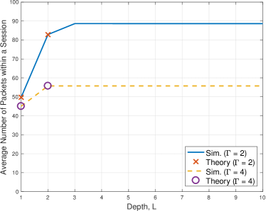
Figure 3: Average number of transmitted packets in a session time (i.e., $W_{\rm S}$ slots) for different values of depth, $L$, when $\Gamma\in\{2,4\}$, $\Omega=20$, $W=50$, and $W_{\rm S}=55$.

Fig. 4 shows the session error probabilities and their ratio/NOMA factor as functions of power budget, $\Omega$, when $\Gamma=4$, $W=50$, and $W_{\rm S}=55$. It is shown that the improvement of the session error probability of OMA is slow as $\Omega$ increases. However, the session error probability significantly decreases with $\Omega$ if opportunistic NOMA mode is employed, which clearly demonstrates that opportunistic NOMA mode is an attractive scheme for SMDDC over fading channels. In Fig. 4 (a), it is shown that the bound in (52) can successfully predict the decreases of the session error probability when opportunistic NOMA mode is used. In addition, we also see that the performance with $L=2$ is almost the same as that with $L=3$, which means that the depth $L=2$ is sufficient to take advantage of opportunistic NOMA mode. In Fig. 4 (b), the NOMA factor, $\eta$, in (55) is shown with the session error probability ratio from simulation results (which is represented by the dashed line).

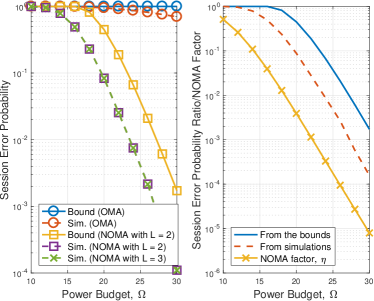
(a)                               (b)

Figure 4: Session error probabilities and their ratio/NOMA factor as functions of power budget, $\Omega$, when $\Gamma=4$, $W=50$, and $W_{\rm S}=55$: (a) session error probability versus $\Omega$; (b) session error probability ratio/NOMA factor versus $\Omega$.

Fig. 5 shows the session error probabilities and their ratio/NOMA factor as functions of session length, $W_{\rm S}$, when $\Gamma=4$, $W=50$, and $\Omega=20$. It is clearly shown that the increase of $W_{\rm S}$ decreases the session error probability at the cost of increasing delay.

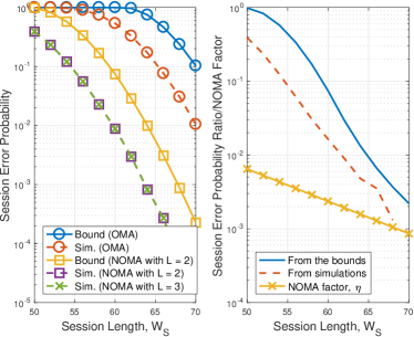
(a)                               (b)

Figure 5: Session error probabilities and their ratio/NOMA factor as functions of session length, $W_{\rm S}$, when $\Gamma=4$, $W=50$, and $\Omega=20$: (a) session error probability versus $W_{\rm S}$; (b) session error probability ratio/NOMA factor versus $W_{\rm S}$.

Fig. 6 shows the session error probabilities and their ratio/NOMA factor as functions of target SINR, $\Gamma$, when $\Omega=10$, $W=50$, and $W_{\rm S}=55$. As the target SINR decreases, the session error probabilities decrease. However, since the code or transmission rate decreases with the target SINR, the target SINR cannot be low. With $\Gamma=2$, we can see that the session error probability of OMA is almost 1, while that with opportunistic NOMA mode becomes sufficiently low (i.e., less than $10^{-2}$). This again shows that opportunistic NOMA mode can play a key role in SMDDC as it can make the session error probability sufficiently low with a reasonably delay constraint.

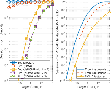
(a)                               (b)

Figure 6: Session error probabilities and their ratio/NOMA factor as functions of target SINR, $\Gamma$, when $\Omega=10$, $W=50$, and $W_{\rm S}=55$: (a) session error probability versus $\Gamma$; (b) session error probability ratio/NOMA factor versus $\Gamma$.

VI-B Results of Asymmetric NOMA

In this subsection, we present simulation results of asymmetric NOMA with SDO-NOMA and FO-NOMA.

Fig. 7 shows the session error probabilities of SDO-NOMA and FO-NOMA as functions of power budget, $\Omega$, when $\Gamma=4$, $K=3$, $W=50$, and $W_{\rm S}=55$. From simulation results (with the two dashed lines), we can see that there is no significant performance difference between SDO-NOMA and FO-NOMA, which means that with a reasonable power budget, it is unlikely to transmit more than two packets using FO-NOMA mode.

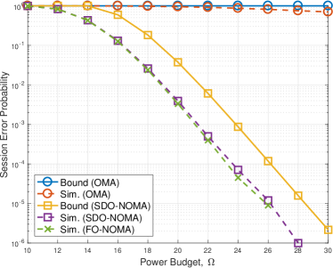
Figure 7: Session error probabilities of SDO-NOMA and FO-NOMA as functions of power budget, $\Omega$, when $\Gamma=4$, $K=3$, $W=50$, and $W_{\rm S}=55$.

The session error probability versus $W_{\rm S}$ is illustrated in Fig. 8 when $\Gamma=4$, $\Omega=15$, $K=3$, and $W=50$. It is noteworthy that even if $W_{\rm S}=W=50$, SDO-NOMA and FO-NOMA can provide a low session error probability, which is about $0.05$, while the session error probability of OMA is 1. With $W_{\rm S}=60$, the session error probability of SDO-NOMA or FO-NOMA can approach $10^{-4}$.

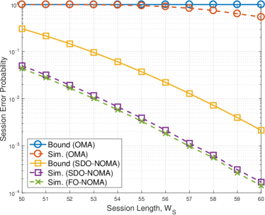
Figure 8: Session error probabilities of SDO-NOMA and FO-NOMA as functions of session length, $W_{\rm S}$, when $\Gamma=4$, $\Omega=15$, $K=3$, and $W=50$.

Fig. 9 shows the session error probabilities of SDO-NOMA and FO-NOMA as functions of the number of radio resource blocks, $K$, when $\Gamma=4$, $\Omega=15$, $W=50$, and $W_{\rm S}=55$. We can see that the session error probability decreases with $K$ in SDO-NOMA due to the increase of the selection diversity gain and in FO-NOMA due to the increase of radio resource blocks to transmit more packets per slot. Note that although FO-NOMA can transmit more packets than SDO-NOMA as $K$ increases (FO-NOMA can transmit up to $K$ packets per slot, while SDO-NOMA can transmit up to two packets per slot), there is no significant performance difference between SDO-NOMA and FO-NOMA in terms of the session error probability. This implies that the impact of the selection diversity gain in SDO-NOMA on the session error probability is similar to that of up to $K-1$ transmissions per slot.

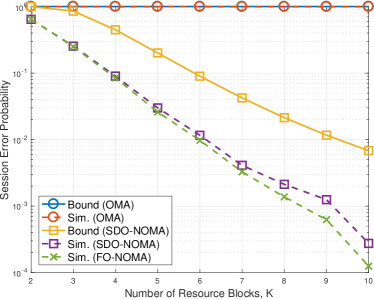
Figure 9: Session error probabilities of SDO-NOMA and FO-NOMA as functions of the number of radio resource blocks, $K$, when $\Gamma=4$, $\Omega=15$, $W=50$, and $W_{\rm S}=55$.

VII Concluding Remarks

In this paper, we studied opportunistic NOMA mode for SMDDC. It was assumed that each user has a set of $W$ packets that are to be transmitted within $W_{\rm S}$ slots for SMDDC. With OMA, it was shown that $W_{\rm S}$ has to be larger than $W$ for a low session error probability, which results in a long delay. On the other hand, it was shown that opportunistic NOMA mode can dramatically lower the session error probability compared with OMA. In particular, under independent Rayleigh fading, with $(W,W_{\rm S})=(50,60)$, it was shown that the session error probability of opportunistic NOMA can approach $10^{-4}$, while that of OMA is 0.5. It was also confirmed by the derived NOMA factor that shows the session error probability of opportunistic NOMA can be significantly lower than that of OMA although $W_{\rm S}$ is not significantly larger than $W$.

There are issues to be investigated in the future. Although an upper-bound on the session error probability was found as a closed-form expression to see the behavior of the session error probability, it was noted that there is a gap between the upper-bound and simulation results. Thus, it is desirable to find a tighter bound in the future. In addition, it is necessary to study the impact of imperfect CSI on SIC, which results in degraded performance (in the paper, we assumed no errors in SIC thanks to perfect CSI).

References

- [1] L. Dai, B. Wang, Y. Yuan, S. Han, C. I, and Z. Wang, “Non-orthogonal multiple access for 5G: solutions, challenges, opportunities, and future research trends,” IEEE Communications Magazine, vol. 53, pp. 74–71, September 2015.
- [2] Z. Ding, Y. Liu, J. Choi, M. Elkashlan, C. L. I, and H. V. Poor, “Application of non-orthogonal multiple access in LTE and 5G networks,” IEEE Communications Magazine, vol. 55, pp. 185–191, February 2017.
- [3] J. Choi, “NOMA: Principles and recent results,” in 2017 International Symposium on Wireless Communication Systems (ISWCS), pp. 349–354, Aug 2017.
- [4] J. Choi, “On generalized downlink beamforming with NOMA,” J. Communications and Networks, vol. 19, pp. 319–328, August 2017.
- [5] L. Dai, B. Wang, Z. Ding, Z. Wang, S. Chen, and L. Hanzo, “A survey of non-orthogonal multiple access for 5G,” IEEE Communications Surveys Tutorials, vol. 20, pp. 2294–2323, thirdquarter 2018.
- [6] Y. Saito, Y. Kishiyama, A. Benjebbour, T. Nakamura, A. Li, and K. Higuchi, “Non-orthogonal multiple access (NOMA) for cellular future radio access,” in Vehicular Technology Conference (VTC Spring), 2013 IEEE 77th, pp. 1–5, June 2013.
- [7] B. Kim, S. Lim, H. Kim, S. Suh, J. Kwun, S. Choi, C. Lee, S. Lee, and D. Hong, “Non-orthogonal multiple access in a downlink multiuser beamforming system,” in MILCOM 2013 - 2013 IEEE Military Communications Conference, pp. 1278–1283, Nov 2013.
- [8] J. Choi, “H-ARQ based non-orthogonal multiple access with successive interference cancellation,” in IEEE GLOBECOM 2008 - 2008 IEEE Global Telecommunications Conference, pp. 1–5, Nov 2008.
- [9] J. Choi, “Effective capacity of NOMA and a suboptimal power control policy with delay QoS,” IEEE Trans. Communications, vol. 65, pp. 1849–1858, April 2017.
- [10] F. Shrouf, J. Ordieres, and G. Miragliotta, “Smart factories in industry 4.0: A review of the concept and of energy management approached in production based on the internet of things paradigm,” in 2014 IEEE International Conference on Industrial Engineering and Engineering Management, pp. 697–701, Dec 2014.
- [11] M. Dixit, J. Kumar, and R. Kumar, “Internet of things and its challenges,” in 2015 International Conference on Green Computing and Internet of Things (ICGCIoT), pp. 810–814, Oct 2015.
- [12] M. Lom, O. Pribyl, and M. Svitek, “Industry 4.0 as a part of smart cities,” in 2016 Smart Cities Symposium Prague (SCSP), pp. 1–6, May 2016.
- [13] M. Z. Shafiq, L. Ji, A. X. Liu, J. Pang, and J. Wang, “A first look at cellular machine-to-machine traffic: Large scale measurement and characterization,” SIGMETRICS Perform. Eval. Rev., vol. 40, pp. 65–76, June 2012.
- [14] A. Sehati and M. Ghaderi, “Online energy management in iot applications,” in IEEE INFOCOM 2018 - IEEE Conference on Computer Communications, pp. 1286–1294, April 2018.
- [15] N. Naik, “Choice of effective messaging protocols for IoT systems: MQTT, CoAP, AMQP and HTTP,” in 2017 IEEE International Systems Engineering Symposium (ISSE), pp. 1–7, Oct 2017.
- [16] D. Kim, H. Lee, and D. Kim, “Enhanced industrial message protocol for real-time IoT platform,” in 2018 International Conference on Electronics, Information, and Communication (ICEIC), pp. 1–2, Jan 2018.
- [17] D. Tse and P. Viswanath, Fundamentals of Wireless Communication. Cambridge University Press, 2005.
- [18] S. Lin and D. J. Costello, Jr, Error Control Coding: Fundamentals and Applications. Englewood Cliffs, N.J.: Prentice Hall, 1983.
- [19] Y. Liu, M. Derakhshani, and S. Lambotharan, “Outage analysis and power allocation in uplink non-orthogonal multiple access systems,” IEEE Communications Letters, vol. 22, pp. 336–339, Feb 2018.
- [20] J. Cui, Z. Ding, and P. Fan, “Outage probability constrained MIMO-NOMA designs under imperfect CSI,” IEEE Trans. Wireless Communications, vol. 17, pp. 8239–8255, Dec 2018.
- [21] J. Choi, “Non-orthogonal multiple access in downlink coordinated two-point systems,” IEEE Commun. Letters, vol. 18, pp. 313–316, Feb. 2014.
- [22] Z. Ding, Z. Yang, P. Fan, and H. Poor, “On the performance of non-orthogonal multiple access in 5G systems with randomly deployed users,” IEEE Signal Process. Letters, vol. 21, pp. 1501–1505, Dec 2014.
- [23] T. M. Cover and J. A. Thomas, Elements of Information Theory. NJ: John Wiley, second ed., 2006.
- [24] D. J. C. MacKay, Information Theory, Inference, and Learning Algorithms. Cambridge University Press, 2003.
- [25] Y. Polyanskiy, H. V. Poor, and S. Verdu, “Channel coding rate in the finite blocklength regime,” IEEE Trans. Information Theory, vol. 56, pp. 2307–2359, May 2010.
- [26] G. Durisi, T. Koch, and P. Popovski, “Toward massive, ultrareliable, and low-latency wireless communication with short packets,” Proceedings of the IEEE, vol. 104, pp. 1711–1726, Sept 2016.
- [27] H. A. David, Order Statistics. New York: John Wiley & Sons, 1980.
- [28] M. Mitzenmacher and E. Upfal, Probability and Computing: Randomized Algorithms and Probability Analysis. Cambridge University Press, 2005.
- [29] R. Arratia and L. Gordon, “Tutorial on large deviations for the binomial distribution,” Bulletin of Mathematical Biology, vol. 51, no. 1, pp. 125 – 131, 1989.
- [30] A. Dembo and O. Zeitouni, Large Deviations Techniques and Applications. Applications of mathematics, Springer, 1998.
- [31] P. Bullen, Handbook of Means and Their Inequalities. Mathematics and Its Applications, Springer Netherlands, 2013.
- [32] S. Schaible, “Fractional programming: Applications and algorithms,” European Journal of Operational Research, vol. 7, no. 2, pp. 111 – 120, 1981. Fourth EURO III Special Issue.