An optical and X-ray study of the contact binary, BH Cassiopeiae

Abstract

We present the revised and high quality CCD time series observations in 2017 and 2018 of the W UMa-type contact binary BH Cas. The combination of our new determinations of minimum times and those collected from the literatures reveal a long-term period increase with a rate of $\textit{dP/dt}\,=\,+3.27\times 10^{-7}\textrm{day}\,\textrm{yr}^{-1}$, which can be accounted for by angular momentum transfer as the less-massive component loses its mass to the more massive one. One cyclical oscillation ($A^{\prime}=0.00300$ day and $P^{\prime}=20.09$ yr) superimposed on the long-term period increase tendency is attributed to one additional object that orbits BH Cas. The low-resolution spectra of this source are observed at phase $\sim$0.0 and $\sim$0.5 in 2018 and 2019, and the spectral types are identified as K3V$\,\pm\,$1 and G8V$\,\pm\,$2. According to the luminosity contributions and spectra at these phases, the spectral type of the primary star is close to K3V$\,\pm\,$1. We infer a cool spot on the hotter and less-massive component to fit the asymmetry of light curves. In addition, changes in the location, temperature, and area of spots on the secondary star in different observations may indicate that the magnetic field activity of the secondary is more active than that of the primary. Such strong spot activities and optical flare are both detected at the same time from a W UMa-type star for the first time. With the XMM-Newton observations taken in 2003 and 2012, the X-ray light curve is obtained and the X-ray spectra can be well described with a black-body or a bremsstrahlung model. The soft X-ray luminosity of BH Cas is estimated as 8.8 – 9.7$\,\times\,10^{30}$ erg s^-1.

1 Introduction

Close binaries are divided into Algol (EA), $\beta$ Lyrae (EB) and W UMa (EW) types (Molík, 1998) according to the shape of their light curves. W UMa-type binaries, which have been studied for more than one century (Müller, 1903), are one of the EW-type with a relatively high frequency of occurrence (Shapley, 1948; Nef & Rucinski, 2008). Many phenomena, however, remain unexplained. For example, the O’Connell effect (O’Connell, 1951; Milone, 1968) shows two maxima times of the light curves with different luminosities. Based on the temperatures and masses, the W UMa-type can be further divided into the W-subtype and the A-subtype (Binnendijk, 1970). For the W-subtype, the primary minima of the light curves are caused by the more massive component transiting the less massive hotter one, whereas for the A-subtype, the situation is reverse. These two subtypes of W UMa-type are generally considered to have an evolutionary relationship with each other, but the direction of evolution between them remains controversial. For example, Li et al. (2004), based on the energy transfer in binary systems, infers that the A-subtype is the later evolution stage of the W-subtype. Gazeas & Niarchos (2006), on the other hand, propose the opposite evolutionary sequence by utilizing statistics of the mass and angular momentum of binary systems.

Many W UMa-type binaries are X-ray emitters. Some of their fundamental features, including high chromospheric and coronal activity (Huenemoerder et al., 2006; Hu et al., 2016; Kandulapati et al., 2015), and synchronous fast-rotation common envelopes (Gondoin, 2004; Chen et al., 2006), are believed to be the origin of the X-ray emission. Their X-ray intensities are related to their orbital periods and spectral types (Stȩpień et al., 2001; Chen et al., 2006). The studies of 2MASS J11201034-2201340 (Hu et al., 2016) and VW Cep (Huenemoerder et al., 2006) indicate that the X-ray light curves do not show obvious occultation or modulation as optical light curves do. The investigation of VW Cep and YY Eri (Vilhu & Maceroni, 2007) suggests that in a UMa binary system, the massive component dominates the magnetic activity.

BH Cassiopeiae (RA=00^h21^m21.4^s, Dec=+59^∘09^′05^′′.2, J2000) was recognized by Beljawsky (1931) as a variable star. Kukarkin (1938) classified it as a W UMa-type variable star with a period of $\sim 0.5$ days and an amplitude of $\sim 0.4$ mag. Metcalfe (1999) presented the light curves in U, B and V bands and the radial velocity curves. He obtained basic parameters (e.g., the inclination, temperatures, and fractional luminosity) of BH Cas and further classified it as a W-subtype W UMa system. However, he corrected for data taken with different telescopes by assuming all U band maxima to be approximately equal, thereby preventing him from detection of the O’Connell effect (Zoła et al., 2001). Zoła et al. (2001) carried out additional photometric observations in R and I bands, and found no O’Connell effect. Niarchos et al. (2001) also detected no significant O’Connell effect in their light curves of BH Cas. For the temperature of BH Cas, Metcalfe (1999) derived an effective temperature about $4600\pm 400$ K by the color index, and later concluded the temperature of the secondary star to be $4980\pm 100$ K and the temperature of primary star to be $4790\pm 100$ K. Zoła et al. (2001) set the temperature of the secondary as 6000 K based on a classification spectrum F8$\pm 2$ for BH Cas, and derived the temperature of the primary as $5550\pm 22$ K.

Information regarding the orbital period change is vital in derivation of the physical properties of contact binaries. By conducting the Observed minus Calculated (O$-$C) analysis for BH Cas, Zoła et al. (2001) noted that the parameters of the linear fit for O$-$C analysis (data covering from 1994 to 2001) were positive, and those of the parabolic fit were close to zero. However, Qian (2001) showed the O$-$C to have a significant upward trend with a rate of $dP/dt=+1.17\times 10^{-6}$ d yr^-1 based on the data obtained from 1994 to 1999, and notwithstanding the relatively short time interval of the observations, commented the rate to be unusually large for a binary system. Using data taken from 1994 to 2008, Arranz Heras & Sanchez-Bajo (2009) measured the linear elements to be nearly 0.

In this paper, we report the revised high-quality CCD photometric data of BH Cas, which when supplemented with minimum times in the light curves collected from the literature, led to an improved determination of the physical parameters of the system. New spectral typing provides more reliable estimation on the stellar temperatures than before, whereas the X-ray light curves and spectra set constraints on the emission mechanisms. We present the optical photometric, spectral and X-ray observations of BH Cas in Section 2. The O$-$C analysis, optical light curve fitting, and X-ray spectral fitting are given in Section 3. We discuss our results in Section 4 and give a summary of our work in Section 5.

2 Observations, Data Reductions and Results

2.1 Optical Observation and Data Reduction

2.1.1 Photometry

BH Cas was observed using the Nanshan 1-meter telescope (Song et al., 2016; Ma et al., 2018) of Xinjiang Astronomical Observatory from Oct. 20, 2017 to Dec. 29, 2018. The telescope was equipped with an E2V CCD203-82 (blue) chip CCD camera, which has $4096\times 4136$ pixels, with a pixel size of 1.125 arcsec. A square area of $1200\times 1200$ pixels near the center of the CCD chip was used, corresponding to a field of view of 22^′.5 $\times$ 22^′.5. A set of Johnson-Cousins B, V, R and I filters was used, with typical exposure times of 20 s for B, 15 s for V, 8 s for R and 17 s for I. For all the observations, the same gain, bin values and readout mode were used.

The aperture photometry package PHOT of IRAF is utilized to reduce the CCD data. Figure 1 demonstrates a part of the observed frame, in which the target, comparison and check stars are labeled. The magnitudes and positions of the comparison and check stars are close to BH Cas. The color of the comparison star is almost the same as that of BH  Cas. The coordinates and visual magnitudes of these stars are listed in table 1. For differential magnitudes, the IRAF command pdump is used to derive the instrumental magnitudes and their errors, and helect is used to extract the Heliocentric Julian Date (HJD) of each frame. Then, the new times of the primary (type I) and secondary (type II) minima in different bands, listed in Table 2, are derived by parabolic least-squares fitting to the light curves. We started out with the equation Min.I = (HJD₀) 2449998.6182(3) + 0.^d40589171(5) $\times$ E as per given in Arranz Heras & Sanchez-Bajo (2009) to obtain the orbital phases, but there is a slight shift in phase. Therefore, we chose one of the minimum times we derived as the new HJD₀. The period is preserved, and the revised linear ephemeris becomes,

$$\textmd{Min.I}=(\textmd{HJD${}_{0}$})\,2458124.1950(1)\,+\,0.^{d}40589171(5)\,\times\,E.$$ (1)

Figure 2(a) exhibits the phase-folded optical light curves of BH Cas observed on Oct. 20, 21(black), Dec. 21(red), 2017 and Jan. 4, 5, 6, 7(green), 2018. In each band of the light curves, the data obtained in these three observation seasons deviate more from each other in the phase range from 0.6 to 1.06 compared with that in other phase ranges. We define the primary (MaxI) and secondary (MaxII) maximum as that following the primary and secondary minima, respectively. The MaxI and MaxII magnitudes, both obtained from the same nights by parabolic least-squares fitting to the light curves, are listed in Table 3. It can been seen that the magnitude difference between the amplitude of the primary and the secondary maxima (MaxI-MaxII) change over observations. Note a clear flare event detected on Oct. 21, 2017. Figure 2(b), showing the differential magnitudes between the comparison and the check stars, manifests that the observed variations in the optical light curves of BH Cas are actual and trustworthy.

Table 1: Coordinates and visual magnitudes of the target, comparison and check stars

Stars	$\alpha_{2000}$	$\delta_{2000}$	$V$	$B-V$
			(mag)	($\Delta$mag)
BH Cas(V)	00h21m21.4s	+59∘09′05′′.2	12.77$\pm$0.22	0.49
2MASS J00211690+5912483(C)	00h21m16.9s	+59∘12′48′′.3	12.92$\pm$0.06	0.50
2MASS J00213244+5911504(K)	00h21m32.4s	+59∘11′50′′.4	13.90$\pm$0.03	0.58

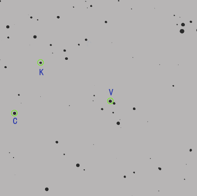
Figure 1: 5.1^′ $\times$ 5.1^′ image in B band. The target BH Cas, the comparison star and the check star are marked, respectively, with “V”, “C” and “K”.

Table 2: New minimum times of BH Cas observed in different bands through this work.

Date	HJD	Type	Error	band	Date	HJD	Type	Error	band
	2400000+					2400000+
2017.10.20	58047.27975	II	0.00024	B	2018.02.07	58157.07476	I	0.00050	B
	58047.27954	II	0.00012	V		58157.07417	I	0.00031	V
	58047.27931	II	0.00037	R		58157.07414	I	0.00032	R
	58047.27912	II	0.00035	I	2018.02.08	58158.08912	II	0.00020	B
2017.10.21	58048.29337	I	0.00025	V		58158.08880	II	0.00017	V
	58048.29293	I	0.00034	R		58158.08922	II	0.00026	R
	58048.29332	I	0.00051	I		58158.08891	II	0.00029	I
2017.12.01	58089.08652	II	0.00044	B	2018.11.03	58426.18572	I	0.00036	B
	58089.08612	II	0.00030	V		58426.18565	I	0.00022	V
	58089.08594	II	0.00089	R		58426.18406	I	0.00020	R
	58089.08641	II	0.00055	I		58426.18561	I	0.00081	I
2017.12.01	58089.28710	I	0.00044	B	2018.11.03	58426.38775	II	0.00044	B
	58089.28772	I	0.00067	V		58426.38691	II	0.00035	V
	58089.28732	I	0.00034	R		58426.38804	II	0.00021	R
	58089.28854	I	0.00079	I		58426.38791	II	0.00077	I
2018.01.04	58123.18243	II	0.00032	B	2018.11.04	58427.20096	I	0.00078	B
	58123.18230	II	0.00022	V		58427.20033	I	0.00049	V
	58123.18175	II	0.00038	R		58427.20074	I	0.00022	R
	58123.18128	II	0.00020	I		58427.20093	I	0.00093	I
2018.01.04	58123.99454	II	0.00032	V	2018.11.04	58427.40276	I	0.00031	B
2018.01.05	58124.19429	I	0.00023	B		58427.40256	I	0.00013	V
	58124.19474	I	0.00016	V		58427.40276	I	0.00073	R
	58124.19505	I	0.00026	R		58427.40318	I	0.00019	I
	58124.19576	I	0.00022	I	2018.11.29	58452.16318	I	0.00094	B
2018.01.06	58125.00740	I	0.00075	B		58452.16351	I	0.00023	V
	58125.00714	I	0.00010	V		58452.16339	I	0.00019	R
	58125.00753	I	0.00086	R		58452.16373	I	0.00051	I
	58125.00835	I	0.00054	I	2018.12.29	58482.19930	I	0.00086	B
2018.01.06	58125.21119	II	0.00030	B		58482.19940	I	0.00068	V
	58125.21102	II	0.00020	V		58482.19951	I	0.00082	R
	58125.20963	II	0.00022	R		58482.19960	I	0.00053	I
	58125.21017	II	0.00021	I
2018.01.07	58126.22427	I	0.00020	B
	58126.22488	I	0.00040	V
	58126.22421	I	0.00080	R
	58126.22455	I	0.00014	I

Table 3: The maximum magnitude values and the magnitude difference between the amplitude of the primary maxima and the following secondary of BH Cas in different bands.

Date	MaxI	Error	MaxII	Error	MaxI-MaxII	Error	band
	($\Delta$mag)		($\Delta$mag)		($\Delta$mag)
2017.12.01	-0.042	0.008	0.039	0.007	0.081	0.015	B
2017.12.01	-0.327	0.008	-0.259	0.009	0.068	0.017	V
2017.12.01	-0.538	0.009	-0.480	0.006	0.058	0.015	R
2017.12.01	-0.721	0.010	-0.682	0.006	0.039	0.016	I
2018.01.04	-0.034	0.005	-0.001	0.010	0.033	0.015	B
2018.01.04	-0.333	0.005	-0.301	0.008	0.032	0.013	V
2018.01.04	-0.534	0.005	-0.503	0.007	0.031	0.013	R
2018.01.04	-0.718	0.004	-0.701	0.008	0.017	0.013	I
2018.01.05	-0.047	0.008	0.011	0.006	0.058	0.014	B
2018.01.05	-0.325	0.007	-0.289	0.004	0.036	0.012	V
2018.01.05	-0.534	0.010	-0.498	0.003	0.036	0.013	R
2018.01.05	-0.724	0.006	-0.690	0.004	0.034	0.010	I

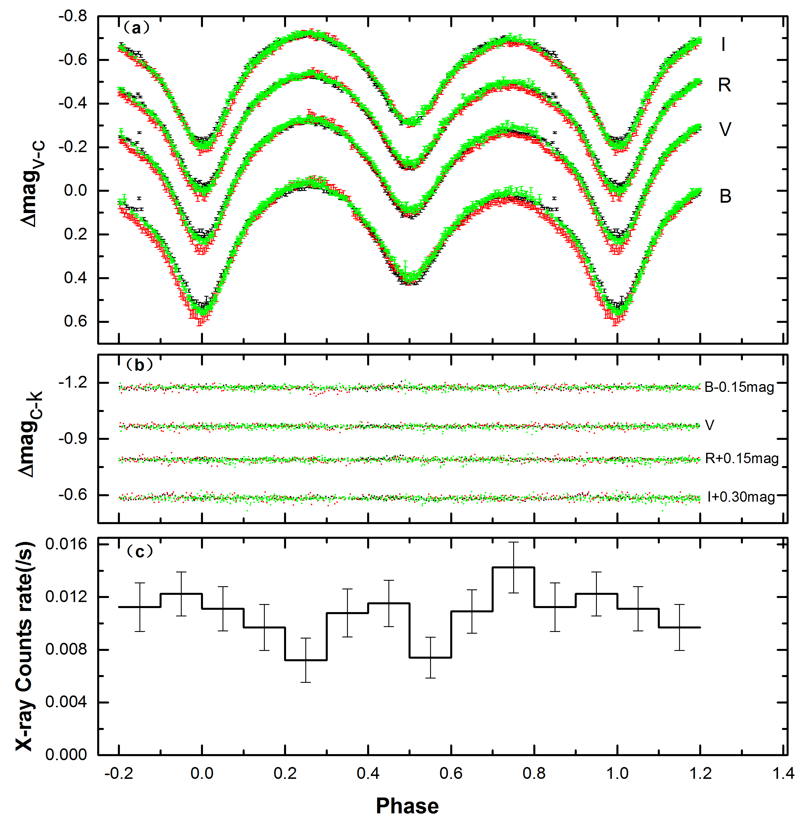
Figure 2: (a): BVRI bands phase-folded light curves for BH Cas. The error bars are set as 2$\sigma$ instrumental magnitudes uncertainties. A clear flare was detected in Oct. 21, 2017. (b): The magnitude differences of the comparison (C) and the check star (K). These colors represent the same meaning as panel (a). (c): The phase-folded X-ray light curve obtained by XMM-Newton in the 0.2–12keV energy range (Section 2.2). The error bars are 1$\sigma$ statistical uncertainties.

2.1.2 Spectroscopy

The low-resolution spectra of BH Cas were observed on November 22, 2018 and January 23, 2019 with the 2.16-meter telescope (Fan et al., 2016) in the Xinglong Observatory, National Astronomical Observatories of China. The Beijing Faint Object Spectrograph and Camera, equipped with a 2048 $\times$ 2048 pixels E2V CCD42-40 NIMO CCD, was used in these observations. A slit of 1.8^′′ and grating G4 was used to provide a wavelength coverage from 3800 Åto 8800 Å, a linear dispersion of 198 Å mm^-1, and a spectral resolution of 4.45 Å pixel^-1. The total exposure time on the target was 800 s. IRAF is used for data reduction following standard spectral processing. Finally, the one-dimension spectra of BH Cas and the standard star Hiltner 102 (Stone, 1974) were extracted for flux calibration. In Figure 3 and 4, the spectra presented by solid black lines are observed at phases $\sim$0.0 (HJD 2458445.067365) and $\sim$0.5 (HJD 2458506.948262), respectively. The spectra were compared with SDSS/BOSS reference spectra of different spectral types from Covey et al. (2007). The PyHammer code (Kesseli et al., 2017) was used to make the comparison, leading to the best fit of K3V$\pm$1 ($\sim$4850$\pm$150 K) and G8V$\pm$2 (Cox, 2000; Harmanec, 1988, $\sim$5300$\pm$300 K), both with [Fe/H]$\sim-1.0$ at phases 0.0 and 0.5, respectively. The positions of absorption lines H$\alpha$ (6564.6127Å), H$\beta$ (4862.6778Å), H$\gamma$ (4341.6803Å) and triple lines (8498Å, 8542Å and 8662Å) of CaII on the spectrum are represented by dashed lines.

According to geometric configuration (Zoła et al., 2001; Metcalfe, 1999) of BH Cas, if we assume that two components are black bodies, the spectral temperature at phase 0.0 is the closest temperature to the primary through the whole phase range while that at phase 0.5 is the closest to the secondary. And since the light curves of BH Cas can be well fitted for a wide range of temperatures (Zoła et al., 2001), the reliable initial values are important for the solution of light curve fitting. Therefore, it is reasonable to set the temperatures 4850 K and 5300 K derived by the spectrum of BH Cas at phases 0.0 and 0.5 as the initial temperatures of the primary and secondary in optical light curve fitting in Section 3.2, respectively.

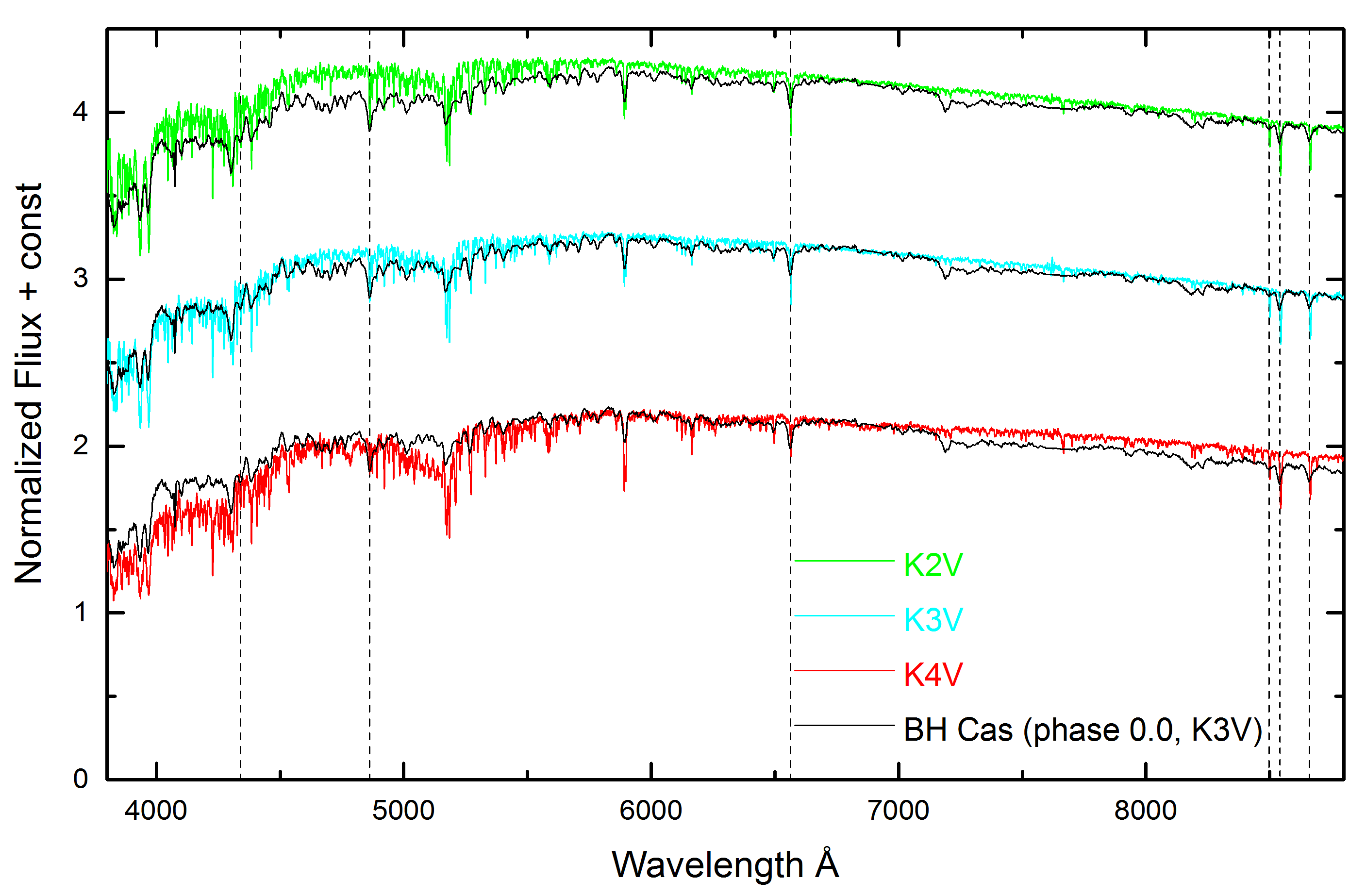
Figure 3: Spectrum of BH Cas at phase 0.0 compared with reference spectra of K2V–K4V. Best fit is obtained for K3V star with [Fe/H]$\,\sim\,-$1.0. All spectra are normalized at $\lambda$=6900Å. From left to right, the black dashed lines represent H$\gamma$ (4341.6803Å), H$\beta$ (4862.6778Å), H$\alpha$ (6564.6127Å) and triple lines (8498Å, 8542Å and 8662Å) of CaII.

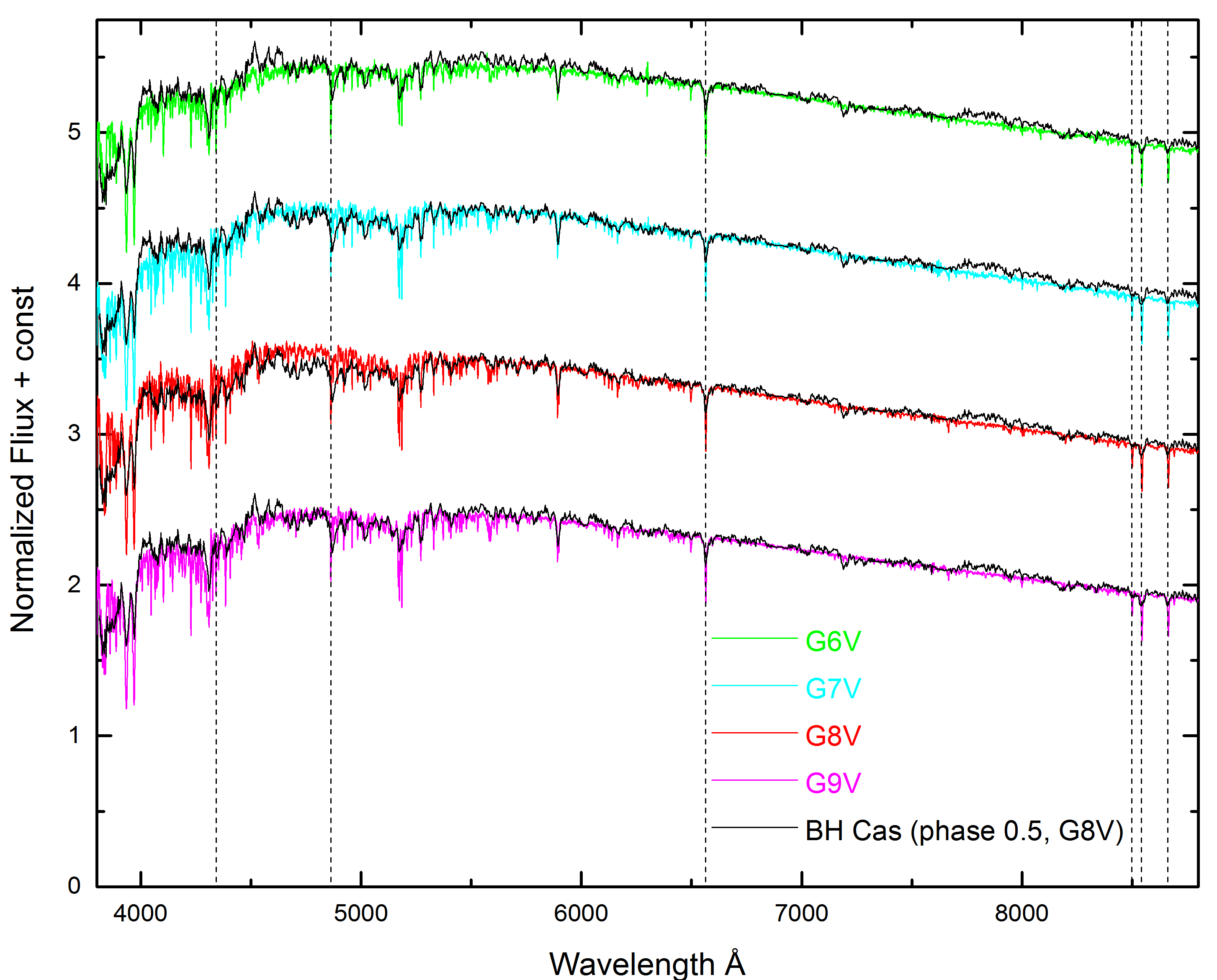
Figure 4: Spectrum of BH Cas at phase 0.5 compared with reference spectra of G6V–G9V. Best fit is obtained for G8V star with [Fe/H]$\,\sim\,-$1.0. All spectra are normalized at $\lambda$=6900Å. From left to right, the black dashed lines represent H$\gamma$ (4341.6803Å), H$\beta$ (4862.6778Å), H$\alpha$ (6564.6127Å) and triple lines (8498Å, 8542Å and 8662Å) of CaII.

2.2 X-ray Observations and Data Reduction

The X-ray detection of BH Cas was firstly presented by Brandt et al. (1997) as a part of the X-ray observations of the Local Group galaxy IC 10. Later, XMM-Newton (Jansen et al., 2001) observed BH Cas with an $\sim 40$ ks exposure on July 3, 2003 with ObsID: 0152260101 and $\sim 130$ ks exposure on August 18, 2012 with ObsID: 0693390101 (Pasham et al., 2013). We downloaded the data from XMM-Newton Science Archive(XSA). All the European Photon Imaging Cameras (EPICs), including two MOS cameras and PN CCD, were operated in the full-frame mode with thin filters in these two observations. Details are listed in Table 4. In the following, we denote the X-ray observations in 2003 and 2012 as O₀₃ and O₁₂, respectively (see Table 4).

We use XSA online Interacting Data Analysis (IDA) to perform pipeline data reduction. IDA processes the observation data files (ODF) with Science Analysis System (SAS) and current calibration files on the Remote Interface for Science Analysis (RISA) server. The system automatically generates filtered events lists, clean spectra and light curves. We extract source photons from a circular region centered on BH Cas with a radius of 30$\arcsec$ to encircle  80% of source energy. BH Cas lies on the boundary of two chips of the PN camera in O₁₂, so we do not use it. The background events are extracted from a source-free 80$\arcsec$ circle near the source. In order to eliminate the difference in results that may be caused by background selection, we also select the source-free backgrounds of other sizes and positions, and find almost no difference in background events after normalization. We do not take the pile-up effect into consideration, because the counts rate of BH Cas $\sim 0.01$ counts s^-1 is far less than the minimum of EPICs needed for consideration. For the event pattern and flag, the options are set to be ”$\textrm{Pattern}\,<=\,12$” and ”Flag = 0” for MOS, respectively, and ”$\textrm{Pattern}\,<=\,4$”, ”Flag = 0” for PN. The energy range is selected to be between 0.2 keV to 12 keV. For the product type, firstly, we set the option to be ”Spectra”. The files of source spectra, background spectra, spectral response matrices for O₀₃ and O₁₂ are automatically generated by IDA. Then, the clean light curves of O₀₃ and O₁₂ with a bin of 2000 s are extracted by setting the option to be ”Light curve”.

The ephemeris from Equation 1 is used to calculate the phase of the X-ray light curve. In order to correct the differences in the light arrival times due to the relative locations of the XMM-Newton and the star, the Modified Julian Date (MJD) of the X-ray light curve is converted to HJD. The bin of phase is eventually set to 0.1 to get enough detection significance. We do not obtain the X-ray light curve from O₀₃ since its effective time span is shorter than the orbital period of BH Cas. The phase-folded X-ray light curve of MOS of O₁₂ is shown in Figure 2(c).

Table 4: The XMM-Newton observation log for BH Cas. Columns are organized as the observation ID and the define name of observation, observation instrument, the start and stop time of the observation, total exposure time and the effective exposure time.

Obs.ID	Def.Name	Instrument	Start	Stop	Tot. Expo.	Effective Expo.
			(UT)	(UT)	(ks)	(ks)
0152260101	O03	PN	2003-07-03 18:22:46	2003-07-04 06:30:01	43.635	33.6675
0152260101	O03	MOS1	2003-07-03 18:00:25	2003-07-04 06:34:57	45.272	36.7406
0152260101	O03	MOS2	2003-07-03 18:00:27	2003-07-04 06:35:01	45.274	36.7926
0693390101	O12	MOS1	2012-08-18 22:06:29	2012-08-20 10:14:43	130.094	100.495
0693390101	O12	MOS2	2012-08-18 22:06:29	2012-08-20 10:14:59	130.110	103.974

3 Data fitting

3.1 The O-C Analysis

Ten years have passed since Arranz Heras & Sanchez-Bajo (2009) pointed out that no evidence had been found for any period change of BH Cas. We obtain 67 new minimum times in this work, combining with 94 minimum times collected from published papers and the website O$-$C Gateway , a total of 161 minimum times that cover 24 years from 1994 to 2018 are used for our O$-$C analysis. Equation 1 is used to calculate the (O$-$C)₁ values. An obvious concave upward trend is evidenced in Figure 5(a). Therefore, we add a period derivative quadratic term to fit the data and the period increasing rate is derived to be $dP/dt=+3.27\times 10^{-7}$ d yr^-1. The fit is statistically improved with a reduced $\chi^{2}=34.3$. The corresponding residual $(O-C)_{2}$ is shown in Figure 5(b). The fitting remains poor, as $(O-C)_{2}$ seems to show a distinct quasi-sinusoidal oscillation between epoch $-21000$ and $-11000$, whereas in the interval $-11000$ to 1000, the distribution is more or less flat, with about 65% of the data points below zero. First, we consider the possibility of an elliptical orbit. There are no suitable solutions; either the errors of the fitting parameters are too large, or the derived orbital eccentricity $e$ is greater than 1, i.e., an non-ellipse orbit. Alternatively, we assume a circular orbit and use the following formula (Hoffman et al., 2006):

$$\begin{split}(O-C)_{1}=&c_{0}\,+\,c_{1}\,\times\,E\,+\,c_{2}\,\times E^{2}\\ &\,+\,[a_{1}\,\textmd{cos}(\omega_{1}\,E)+b_{1}\,\textmd{sin}(\omega_{1}\,E)]\\ \end{split}$$ (2)

where c₀, c₁ and c₂ are the parabolic fitting parameters, and a₁, b₁ are the Fourier coefficients. The best-fit parameters are listed in Table 5 with the errors being directly output from the covariant matrix. The revised quadratic ephemeris is then:

$$\begin{split}\textmd{{Min.I}}=&(\textmd{HJD${}_{0}$})\,2458124.19660(25)\\ &\,+\,0.^{d}40589680(8)\,\times{E}\\ &+1^{d}.82(4)\,\times\,10^{-10}\,\times\,E^{2}.\end{split}$$ (3)

In Figure 5(b), we use a red solid line to indicate the oscillation with the amplitude $A^{\prime}=0.00300$ days and the oscillation period $P^{\prime}=2\pi P/\omega=20.09$ yr. The residuals in Figure5 (c) represent the deviation of data points in panel (b) from the red solid line. The best-fit parameters of this oscillation are listed in Table 5. The reduced $\chi^{2}$ is 17.3 in Figure 5 (c).

Table 5: Best fit orbital parameters for BH Cas.

Date	Values	Error
c0	1.60 $\times$ 10-3	2.5 $\times$ 10-4
c1	5.09 $\times$ 10-6	8 $\times$ 10-8
c2	1.82 $\times$ 10-10	4 $\times$ 10-12
a1	5.10 $\times$ 10-5	1.9 $\times$ 10-6
b1	3.00 $\times$ 10-3	2.8 $\times$ 10-4
$\omega_{1}$	3.47 $\times$ 10-4	6 $\times$ 10-6

Figure 5: (a): The $(\rm O-\rm C)_{1}$ diagram for BH Cas. Observed data are represented by red (literature) or blue (this work) points. The black dashed line is the parabolic least-squares fit (first three terms of Equation (2)) to the data. (b): The $(\rm O-\rm C)_{2}$ diagram (subtracting the dashed line from the observations in (a)). The red solid line is the fit to the data by $[a_{1}\,\textmd{cos}(\omega_{1}\,E)+b_{1}\,\textmd{sin}(\omega_{1}\,E)]$ with amplitude A^′ = 0.00300 days and oscillation period P ^′ = 20.09 yr and also plotted in panel (a) (black solid line) by adding to the black dashed line.(c): The residuals of panel(b). The distributions of our data at the ephemeral scale, in panel (a), (b) and (c), are zoomed in panel (d), (e) and (f), respectively.

3.2 Optical Light Curve Model Fitting

The 2013 version of the Wilson-Devinney (W-D) code (Wilson & Devinney 1971;Wilson 1979; Wilson 2012) is used to fit the light curves in four bands in order to get the physical and geometrical parameters of BH Cas. In the fitting process, we use the photometric data of this work and the radial velocity of Metcalfe (1999) as the constraint condition. We define the primary component with subscript 1 and the secondary with subscript 2. In our fitting, the mass ratio q ($M_{2}/M_{1}$)= 0.475(23) obtained by radial velocity measurements (Metcalfe, 1999) is fixed through the fitting. The initial values of mean temperature of the primary (T₁) and secondary (T₂) are set to be 4850 K and 5300 K as mentioned in Section 2.1.2. A circular orbit and synchronous rotation are assumed. For the bolometric and monochromatic limb darkening law, we use the logarithmic form with the coefficients, X_bolo, Y_bolo, x_B, y_B, x_V, y_V, x_R, y_R, x_I and y_I taken from van Hamme (1993). The gravity darkening coefficients and the bolometric albedos are set to g₁ = g₂ = 0.32 (Lucy, 1967) and A₁ = A₂ = 0.50 (Ruciński, 1969) because the atmospheres should both be convective. The adjustable parameters are: the orbit inclination i, the mean surface temperature of primary T₁, the mean surface temperature of secondary T₂, the modified dimensionless surface potential $\Omega$₁, and the bandpass luminosity of primary L₁.

As shown in Figure 5(b), there is a cyclic modulation in the orbital period variation of BH Cas. So the third light L₃ is taken into consideration in the light curves fitting. Because of the asymmetry of the light curves and the unequal luminosities at the maximum times (see Figure 2), it is impossible to get perfect fitting to the light curves without star spots. After a series of iterations we obtain fair solutions by adding a cool spot on the secondary star by adjusting the longitude, latitude, angular radius and temperature of the spot. These solutions are listed in Table 6. The parameters of BH Cas yielded by three sets of photometric solutions are almost identical. In Figure 6, the theoretical light curves given by the solution are compared to the observed ones in different observations. Figure 7 illustrates the geometric structure of BH Cas at different orbital phases with a spot on the secondary component in different observations. The revised absolute parameters we obtained for BH Cas are listed in Table 7. We should note that the errors in Table 6 and 7 are most likely underestimated (Prša & Zwitter, 2005). The reason is the existence of strong correlation between the fitted parameters due to due to the parameter space degeneracy of the model used.

Figure 6: Comparing of observed (open circles) and theoretical (solid lines) light curves in BVRI of BH Cas in different observations. The red solid points in panel (a) represent the optical flare.

Figure 7: The geometric configuration of BH Cas with a spot in the less-massive component at phases 0.00, 0.06, 0.62 and 0.75 in different observations.

Table 6: BVRI band photometric solutions of BH Cas obtained in October 2017, December 2017 and January 2018

Parameters	Best-fit Value(2017.10)	Best-fit Value(2017.12)	Best-fit Value(2018.01)
	Primary               Secondary	Primary               Secondary	Primary               Secondary
$g1=g2$ (deg)	0.32	*	*
$A1=A2$ (deg)	0.50	*	*
$X_{bolo}$	0.649                     0.647	*                     *	*                     *
$Y_{bolo}$	0.193                     0.221	*                     *	*                     *
$x_{B}$	0.847                     0.829	*                     *	*                     *
$y_{B}$	0.098                     0.185	*                     *	*                     *
$x_{V}$	0.778                     0.745	*                     *	*                     *
$y_{V}$	0.200                     0.256	*                     *	*                     *
$x_{R}$	0.686                     0.653	*                     *	*                     *
$y_{R}$	0.230                     0.267	*                     *	*                     *
$x_{I}$	0.591                     0.560	*                     *	*                     *
$y_{I}$	0.229                     0.256	*                     *	*                     *
$i$ (deg)	71.51(85)	70.86(53)	70.91(67)
$q$=$M_{2}/M_{1}$	0.475	*	*
$T$(K)	4899(124)              5109(139)	4862(64)                5214(65)	4874(66)                5163(74)
$\Omega$	2.784(3)                 2.784(3)	2.783(2)                 2.783(2)	2.783(2)                 2.783(2)
$L_{1}/(L_{1}+L_{2})_{B}$	0.589(3)	0.548(3)	0.565(3)
$L_{1}/(L_{1}+L_{2})_{V}$	0.605(3)	0.572(3)	0.587(3)
$L_{1}/(L_{1}+L_{2})_{R}$	0.618(3)	0.592(3)	0.602(3)
$L_{1}/(L_{1}+L_{2})_{I}$	0.625(3)	0.604(3)	0.613(3)
$L_{3}/(L_{1}+L_{2}+L_{3})_{B}$	$2.18(9)\times 10^{-3}$	$2.04(6)\times 10^{-3}$	$2.26(8)\times 10^{-3}$
$L_{3}/(L_{1}+L_{2}+L_{3})_{V}$	$4.11(17)\times 10^{-4}$	$3.92(9)\times 10^{-4}$	$4.32(10)\times 10^{-4}$
$L_{3}/(L_{1}+L_{2}+L_{3})_{R}$	$1.39(19)\times 10^{-5}$	$1.64(13)\times 10^{-5}$	$1.52(11)\times 10^{-5}$
$L_{3}/(L_{1}+L_{2}+L_{3})_{I}$	$6.14(21)\times 10^{-6}$	$5.74(17)\times 10^{-6}$	$5.93(19)\times 10^{-6}$
$r$(pole)	0.4255(4)              0.3030(4)	0.4287(2)              0.3063(2)	0.4275(3)              0.3051(3)
$r$(side)	0.4539(6)              0.3172(6)	0.4581(3)              0.3213(3)	0.4566(4)              0.3198(4)
$r$(back)	0.4844(8)              0.3547(9)	0.4901(5)              0.3614(4)	0.4880(5)              0.3589(6)
Latitudespot(deg)	136.19(40.86)	101.11(2.03)	120.27(31.70)
Longitudespot(deg)	125.64(8.16)	115.98(89)	86.70(14.41)
Radiusspot(deg)	37.80(11.96)	41.12(73)	27.39(48)
$T_{spot}/T_{2}$	0.83(5)	0.80(1)	0.64(9)
$f$(%)	15.14(4)	15.48(4)	15.48(4)

Table 7: Absolute parameters of BH Cas.

Name	M (M${}_{\odot})$	$R$ (R${}_{\odot})$	log g (cgs)	$M_{bol}$	$L$ (L${}_{\odot})$
Primary	0.96(9)	1.19 (7)	4.27(6)	5.01(7)	0.703(13)
Secondary	0.46(6)	0.85(4)	4.24(11)	5.47(8)	0.456(10)

3.3 X-Ray Spectra Fitting

XSPEC version 12.10.0 is used to fit X-ray spectra. Since there are few photons above 2 keV, and X-ray emission is dominated by the background, the fitting is carried out in the energy range 0.2–2 keV, i.e., the soft X-rays. We separately try the thermal bremsstrahlung, black-body and the non-thermal power law to fit the spectra, corresponding to bremss, bbody and powerlaw radiative models in XSPEC. We use the absorption model wabs. The average Galactic hydrogen column density $N_{H}$ in the region near BH Cas is estimated to be $4.82\times 10^{21}$ cm^-2 by the Leiden/Argentine/Bonn Survey (Kalberla et al., 2005). At first, we set $N_{H}$ as a free parameter. The lowest best fit valve is then $6.07^{+1.94}_{-1.54}\,\times\,10^{21}$ cm^-2, which is not far from the derived value but with too large an uncertainty. We then fixed the value of $N_{H}$ as $4.82\,\times\,10^{21}\,\textrm{cm}^{-2}$. We find that the power-law model failed to fit the spectra, with all reduced $\chi^{2}\approx 2$. We separately carried out simultaneous-fitting using bremss or bbody model for each observation. The reduced $\chi^{2}$ values in O₁₂ are all greater than those in O₀₃, which is most likely caused by the exposure times and the instrumental differences between MOS and PN, e.g., quantum efficiency and time resolution (Strüder et al., 2001; Turner et al., 2001). Fitting parameters are listed in Table 8, and the spectra with the corresponding best-fit models are shown in Figure 8. For the black-body and the bremsstrahlung models of O₀₃, the plasma temperatures $\textit{kT}_{\textrm{03}}$ are $0.137^{+0.006}_{-0.006}$ keV and $0.266^{+0.020}_{-0.017}$ keV, respectively, and for O₁₂, they are $0.132^{+0.006}_{-0.006}$ keV and $0.258^{+0.019}_{-0.016}$ keV. The derived X-ray flux in the energy range 0.2–2 keV is estimated to be $\thicksim 3.77^{+0.27}_{-0.28}\,\times\,10^{-14}$ erg cm^-2 s^-1 in 2003, and $\thicksim 4.16^{+0.21}_{-0.21}\,\times\,10^{-14}$ erg cm^-2 s^-1 in 2012.

Table 8: The best fitting parameters for black-body and bremsstrahlung models for the X-ray spectra of BH Cas.

Obs.ID	Parameters	Black Body	Bremsstrahlung
0152260101	$kT\,(\textrm{keV})$	$0.137^{+0.006}_{-0.006}$	$0.266^{+0.020}_{-0.017}$
	Normalization	$6.50^{+1.09}_{-0.97}\,\times\,10^{-6}$	$1.91^{+0.51}_{-0.41}\,\times\,10^{-3}$
	Reduced $\chi^{2}$ (d.o.f )	1.06(74)	1.25(74)
	Absorbed Flux	$3.72^{+0.37}_{-0.38}$	$3.82^{+0.39}_{-0.40}$
	$(\times\,10^{-14}\textrm{erg}\,\textrm{cm}^{-2}\,\textrm{s}^{-1})$
0693390101	$kT\,(\textrm{KeV})$	$0.132^{+0.006}_{-0.006}$	$0.258^{+0.019}_{-0.016}$
	Normalization	$7.95^{+1.33}_{-1.18}\,\times\,10^{-6}$	$2.27^{+0.62}_{-0.51}\,\times\,10^{-3}$
	Reduced $\chi^{2}$ (d.o.f)	1.55(58)	1.84(58)
	Absorbed Flux	$4.12^{+0.29}_{-0.30}$	$4.20^{+0.31}_{-0.29}$
	$(\times\,10^{-14}\textrm{erg}\,\textrm{cm}^{-2}\,\textrm{s}^{-1})$

Figure 8: The X-ray spectra data (crosses) of BH Cas with different Obs.IDs and fitted by different radiation models (steps), PN colored in black, MOS1 colored in red and MOS2 colored in green. (a): Data are obtained in O₀₃ and fitted by black-body model. (b): O₀₃ and bremsstrahlung. (c): O₁₂ and black-body. (d): O₁₂ and bremsstrahlung. All of the lower panels represent the deviation of the data points from the fitting models.

4 Discussions

4.1 Additional Companion

The cyclic oscillation shown in Figure 5 (b) may be caused by the Applegate mechanism (Applegate, 1992), or by the light-time effect as a consequence of the existence of a third body. By calculating the quadrupole moment of the solar-type components, we can quantify the role played by the Applegate mechanism. The equation given by Rovithis-Livaniou et al. (2000):

$$\Delta P=\sqrt{2\,[1-\textmd{$\cos$}(2\pi P/P^{\prime})]}\times A,$$ (4)

where A is the semi-amplitude, P ^′ is the oscillation period , and $\textit{A}\,=\,\sqrt{a_{1}^{2}+b_{1}^{2}}$ = 0.00300 day. By using the relationship between $\omega$ and P ^′, $\omega$ = 2$\pi$P/P ^′, we get the value of P ^′ in year. So the periodic rate of change is $\Delta$P/P $\sim$ 2.568 $\times$ 10^-6. To produce such a change rate, the change in the required quadrupole moment can be calculated using Equation (Lanza & Rodonò, 2002):

$$\Delta P/P\,=\,-9\,\frac{\Delta Q}{Ma^{2}},$$ (5)

where M is the mass of each component in solar mass, and the semi-major axis a is the distance between two components. a can be solved using Kepler’s third law:

$$M_{1}+M_{2}=0.0134\frac{a^{3}}{P^{2}}.$$ (6)

Combining Equations 5 and 6, we then obtain the required quadrupole momentums variations of $\Delta$Q₁ $\sim$ 1.8 $\times$ 10⁴⁹ g cm² and $\Delta$Q₂ $\sim$ 8.8 $\times$ 10⁴⁸ g cm². However, these are less than the range of typical values for a binary system with periodic oscillations that can be explained by this mechanism is 10⁵¹ g cm² to 10⁵² g cm² (Lanza & Rodonò, 2002). In addition, this mechanism is mainly used to explain period modulations of an amplitude $\Delta$P/P $\sim$10^-5(Applegate, 1992) while this value of BH Cas is $\sim$10^-6. Therefore, we conclude that the Applegate mechanism is unable to explain the periodic change of this source. Alternatively, we consider the light-time effect (LITE) to explain the cyclic oscillation. By combining the orbit parameters listed in Table 5, we get the parameters of the third body using the following formula (Kopal, 1978):

$$a\,^{\prime}\,\textmd{sin}i^{\prime}=\textmd{c}\sqrt{a_{1}^{2}+b_{1}^{2}},$$ (7)

where $\textit{a}\,^{\prime}$ is the orbital radius of the common center of mass of the triple system consisting of the contact binary and a third body, and i ^′ is the inclination of the third body. We further calculate the mass of the third object $M\,^{\prime}$ and the orbital radius $a\,^{\prime}$ via:

Table 9: Derived parameters of the third body of BH Cas.

Parameters	Third Body
	Values         Error
P ′ (yr)	20.09            0.14
a ′sini ′ (AU)	0.52             0.06
f $\rm(\textit{M}^{\prime}\rm)$ (M⊙)	3.48 $\times$ 10-4   2.6 $\times$ 10-5
M$\,{}^{\prime}\,$(i ′ = 90 ∘) (M⊙)	0.093           0.007
a$\,{}^{\prime}\,$(i ′ = 90 ∘) (AU)	7.94             0.13

$$f\,\rm(\textit{M}\,^{\prime}\rm)\,=\,\frac{(\textit{M}\,^{\prime}\sin\textit{i}\,^{\prime})^{3}}{(\textit{M}_{1}+\textit{M}_{2}+\textit{M}\,^{\prime})^{2}}\,=\,\frac{4\pi^{2}}{GP^{\prime 2}}(\textit{a}\,^{\prime}\,\sin\textit{i}\,^{\prime})^{3},$$ (8)

$$d\,^{\prime}\,=\,\frac{M_{1}+M_{2}}{M\,^{\prime}}a\,^{\prime},$$ (9)

where G is the gravitational constant. The computed astrometric orbit makes the existence of the LITE evident. The mass of the third object thus derived is 0.098(9) M_⊙ if its orbit is coplanar (i = 71^∘) with the binary system. The derived properties of the third body are listed in Table 9. In addition, the light curve fitting to our observations (see Table 6) shows that the contribution of the third light to the total luminosity reaches two thousandths in B band, which may also support the possible existence of a third body.

4.2 The Magnetic Field Activity

As shown in Table 3, all the magnitudes of maximum times around phase 0.25 are significantly higher than those around 0.75. We thereby conclude that, for the first time, we detect significant O’Connell effect in BVRI bands for BH Cas. As shown in Figure 2(a), we note that the light curves in all bands scatter noticeably from phase 0.6 to 1.06 comparing to that from phase 0.06 to 0.6, and the magnitude difference between the amplitude of the primary maxima and the following secondary changes from season to season. An optical flare was detected on Oct. 21, 2017, and this is the first detection of an optical flare in this source. The variations in the $B$ and $V$ bands, which amount to $\sim 0.15$ mag and continue for $\sim$15 minutes, show the flare near phase 0.85. In R and I bands the tendency also can be recognized. The luminosity of the flare decreases as the wavelength increases, similar to the situation in U Pegasi (Huruhata, 1952). One possible explanation for the O’Connell effect is the magnetic activities, manifest by flares (Qian et al., 2012, 2014) or star spots (McCartney, 1997). But flares are sporadic and short in duration, hence, difficult to account for the persistence of the O’Connell effect. However, star spots are relatively long-lived, and their existence and the distribution on the surface can be diagnosed with photometric observations at different rotational phases. By adding a cool spot on the less massive component, the W-D code fitting leads to a good result for the different luminosity of the maximum times and the asymmetry in optical light curves. In three observation seasons, the variation of the amplitude of the light curves is likely caused by the changes of the total spot area, location, and temperature, i.e. strong spot activities. From the W-D solution, the spot began to appear at phase $\sim$0.6, was completely exposed at phase $\sim$0.75, and was covered by the primary star at phase $\sim$1.06, which are in good agreement with the observations. These variations in the spot of the secondary suggest a stronger magnetic activity than that of the primary. No flare and significant O’Connell effect have been reported in previous works for BH Cas (Metcalfe, 1999; Zoła et al., 2001; Niarchos et al., 2001). Our detections suggest that this source in its stronger magnetic active state during our observations than that of previous observations. In addition, there are shallow absorptions in the H$\alpha$, H$\beta$, H$\gamma$ (Pi et al., 2017) and Ca II triplet lines (Mallik, 1997) in the spectra of Figure 3 and 4. These may indicate that BH Cas is chromospherically active.

4.3 The Spectral Types

Our low-resolution spectra show that the spectral types at phase $\sim$0.0 and $\sim$0.5 are K3V$\pm$1 ($\sim$4850$\pm$150 K) and G8V$\pm$2 ($\sim$5300$\pm$ 300 K), respectively. As shown in Table 6, the temperatures of the primary $T_{1}$ and secondary $T_{2}$ obtained from light-curve fitting are $\sim$4880$\pm$100K ($\sim$K3V$\pm$1) and $\sim$5160$\pm$100 K ($\sim$G9V$\pm$1), respectively. Using the inclination i in Table 6 and absolute parameters listed in Table 7, the geometric model of BH Cas is simplified as two spheres with external tangent. If we do not consider the limb darkening effect, the ratios of luminosities of primary to secondary are derived to be $\sim$7:1 at phase 0.0 and $\sim$1:1 at phase 0.5. This may indicate that the temperature of the primary should be slightly lower than the spectral temperature at phase 0.0 while the temperature of secondary higher than the spectral temperature at phase 0.5. Considering the errors of the light curve fitting are most likely underestimated, the fitting temperature of primary is close to the spectral temperature at phase 0.0, which may be caused by the dominant luminosity of the primary at this phase and may suggest that the spectral type of primary is likely to be $\sim$K3V$\pm$1. According to the light curve fitting, the spectral type of the secondary is $\sim$G9V$\pm$1, while the photometric contribution and the spectral type at 0.5 phase indicated that the temperature of secondary is higher than the spectral temperature of G8V$\pm$2. The inconsistency between these results makes it difficult for us to judge the actual spectral type of the secondary. Considering the magnetic activity of BH Cas mentioned in Section 4.2, the spectrum may be influenced by stellar activities, e.g. spots, flares, resulting in deviation of spectrum temperature from typical stellar temperature of BH Cas.

Metcalfe (1999) derived an effective temperature for BH Cas about 4600$\pm$400 K by the $V-I$ and $R-I$ colors. This temperature corresponds to a main-sequence spectral type K4$\pm$2. Using W-D code, he derived the temperatures of the primary and secondary star as 4790$\pm$100K and 4980$\pm$100K, which are close to the fitting temperatures of this work. A temperature of BH Cas released by Gaia2 is 4990$\pm$324 K(Andrae et al., 2018). Although the uncertainty of the temperature is high, it is within the range of component temperature of BH Cas we derived by spectra. Based on a single spectrum taken in the range 5080 - 5290 Åwith a resolution of 0.2 Å/pixel using a 1.9-m telescope (Lu & Rucinski, 1999), Zoła et al. (2001) set the temperature of secondary component to 6000K according to spectral type of F8($\pm$2). By fixing $T_{2}$ to 6000 K, $T_{1}$=5500 K is obtained using W-D code. The spectral type of F8($\pm$2) is significantly different from what we got at phase of 0.0 or 0.5. Although a strong stellar activity could be a possible reason, we may suggest that such a difference is most possibly due to a high uncertainty in the determining the spectral type using such a narrow range (210Å) and high resolution. More low resolution spectral observations at different phases may help us to explore component spectral types of BH Cas.

4.4 The X-ray Emission

While the variation in the optical light curves is caused by the binary geometry and inclination, the X-ray light curve does not show obvious eclipses. The lack of X-ray variability, with a reduced $\chi^{2}$ of the phase-folded X-ray light curve (Figure 2(c)) being, 1.5, could be the consequence of insufficient number of X-ray photons. Alternatively this indicates a different light distribution of X-ray from that of the optical one. The fitting of asymmetry and O’Connell effect in the optical light curves suggests the presence of spot. The X-ray emission may be caused by the chromosphere and corona activity (Huenemoerder et al., 2006; Hu et al., 2016; Kandulapati et al., 2015). The location, size and temperature of the spot change with time. This change may be reflected in the X-ray light curve or spectra. However, X-ray and optical observations are not carried out at the same time. Simultaneous observations of X-ray and optical are necessary to solve the issue. Both of the single models, the black-body and the bremsstrahlung, can describe the X-ray spectra of BH Cas, which indicates that the origin of X-ray emission of this source is thermal. The derived fluxes in the energy range 0.2–2 keV are estimated to be $\thicksim 3.77^{+0.27}_{-0.28}\,\times\,10^{-14}$ erg cm^-2 s^-1 in 2003, and $\thicksim 4.16^{+0.21}_{-0.21}\,\times\,10^{-14}$ erg cm^-2 s^-1 in 2012. Using the Gaia2 parallax $2.2646\pm 0.0288$ mas (Gaia Collaboration, 2018), the distance of BH Cas is estimated to be 441${}^{+6}_{-5}$ pc. The average X-ray luminosities of BH Cas are then estimated as $L_{03}\,=\,8.76^{+0.63}_{-0.65}\,\times\,10^{29}$ erg s^-1 and $L_{12}\,=\,9.67^{+0.34}_{-0.49}\,\times\,10^{29}$ erg s^-1. In 1997, the X-ray flux of BH Cas in 0.1–2.5 keV is measured to be $4.2\,\times\,10^{-14}$ erg cm^-2 s^-1 (Brandt et al., 1997) and the average X-ray luminosity in this observation is about $9.67\,\times\,10^{29}$ erg s^-1. Although the X-ray flux in the light curve fluctuates between different phases of the complete phase, there is no significant change in these average X-ray luminosities, which indicates that the average X-ray luminosity of BH Cas may be stable over long time.

4.5 Mass Transfer and Evolution of Angular Momentum

The solution of the W-D code, revealing a hotter less-massive component, indicates that BH Cas is a W-subtype W UMa system. Moreover, the O$-$C analysis shows a long-term increase in the orbital period which can be explained by the transfer of matter from the less-massive component to the more-massive one. Using the following equation (Tout & Hall, 1991),

$$\frac{\dot{P}}{P}=3\dot{M_{1}}(\frac{1}{M_{2}}-\frac{1}{M_{1}}),$$ (10)

where the mass of the two components, M₁ = 0.96 M_⊙, M₂ = 0.46 M_⊙, we derive the mass transfer rate d$M_{1}$/dt = +2.37 $\times$ 10^-7 M_⊙/yr. The plus symbol means that the more massive component is gaining mass from the less massive star at a rate of dM₂/dt = $-$2.37 $\times$ 10^-7 M_⊙/yr. The mass transfer time scale is then $\tau$ $\sim$ M₂/$\dot{M_{2}}$ $\sim$ 1.48  $\times$ 10⁶ yr. The coupling of this mass transfer process with the increase of orbital period is consistent with the prediction of the angular momentum loss (AML) theory (e.g., Shengbang & Qingyao (2000)).

The orbital angular momentum and the spin angular momentum (Arbutina, 2007) of binaries can be estimated by

$$J_{orb}\,=\,\frac{M_{1}M_{2}}{M_{1}+M_{2}}a^{2}\Psi,$$ (11)

$$J_{spin}\,=\,k_{1}^{2}M_{1}R_{1}^{2}\Psi_{1}+k_{2}^{2}M_{2}R_{2}^{2}\Psi_{2},$$ (12)

where $\Psi_{i}$s are the orbital angular velocities, $k_{i}^{2}s$ are the dimensionless gyration radii, and $R_{i}s$ are the volume radii. We can assume synchronization for close binaries, so $\Psi_{1}$ = $\Psi_{2}$ = 2$\pi$ / P. Since the possible evolutionary relationship between W-subtype and A-subtype is still controversial, it is reasonable to study their angular momentum evolution separately. In order to investigate the angular momentum of W-subtype binaries, according to their period and total mass, i.e., M₁ + M₂ $<$ 3, and P $<$ 1day, we compile a list of 73 objects for which the absolute parameters have been well determined. Their basic parameters are listed in Table 10, sorted by the decreasing total mass. We derive the values of J_spin/J_orb and J_spin + J_orb for all these binaries. After a series of least-squares fitting in different forms, we obtain the best fitting curves as shown in Figure 9. The equation between $\log(J_{spin}/J_{orb})$ and $\log(q)$ is as follows:

$$\begin{split}\log(J_{spin}/J_{orb})\,=&\,-1.43817-0.08274\times\log(q)\\ &+1.63025\times(\log(q))^{2}\\ &+0.83308\times(\log(q))^{3}\\ &+0.11355\times(\log(q))^{4}.\end{split}$$ (13)

In Figure 9, the green open circles represent the W-subtype W UMa-type contact binaries, and the fitting curve is in black, with the size of each circle corresponding to the value of the angular momentum. In general, as $\log(q)$ decreases, $\log(J_{spin}/J_{orb})$ increases. The cyan square point is the position where $J_{spin}/J_{orb}$ = 1/3, we obtained minimal mass ratio $q_{min,W-subtype}\,=\,0.0757(4)$. This value of the secular tidal instability is consistent with the range 0.076—0.078 reported by Li & Zhang (2006), and is marginally higher than the range 0.070–0.074 presented by Arbutina (2009). Adopting the absolute parameters we obtained for BH Cas, $J_{spin}/J_{orb}=0.04531$. Due to the total mass of BH Cas is small, the angular momentum of BH Cas is smaller than other source around it (see Figure 9). With the transfer of mass between the two components of BH Cas, the mass ratio will decrease, while $J_{spin}/J_{orb}$ increases. If the system reaches a state when $J_{\textrm{orb}}$ = 3 $J_{\textrm{spin}}$ (Arbutina, 2007), tidal instability will occur, thereby forcing the binary to merge into a single, rapidly rotating star.

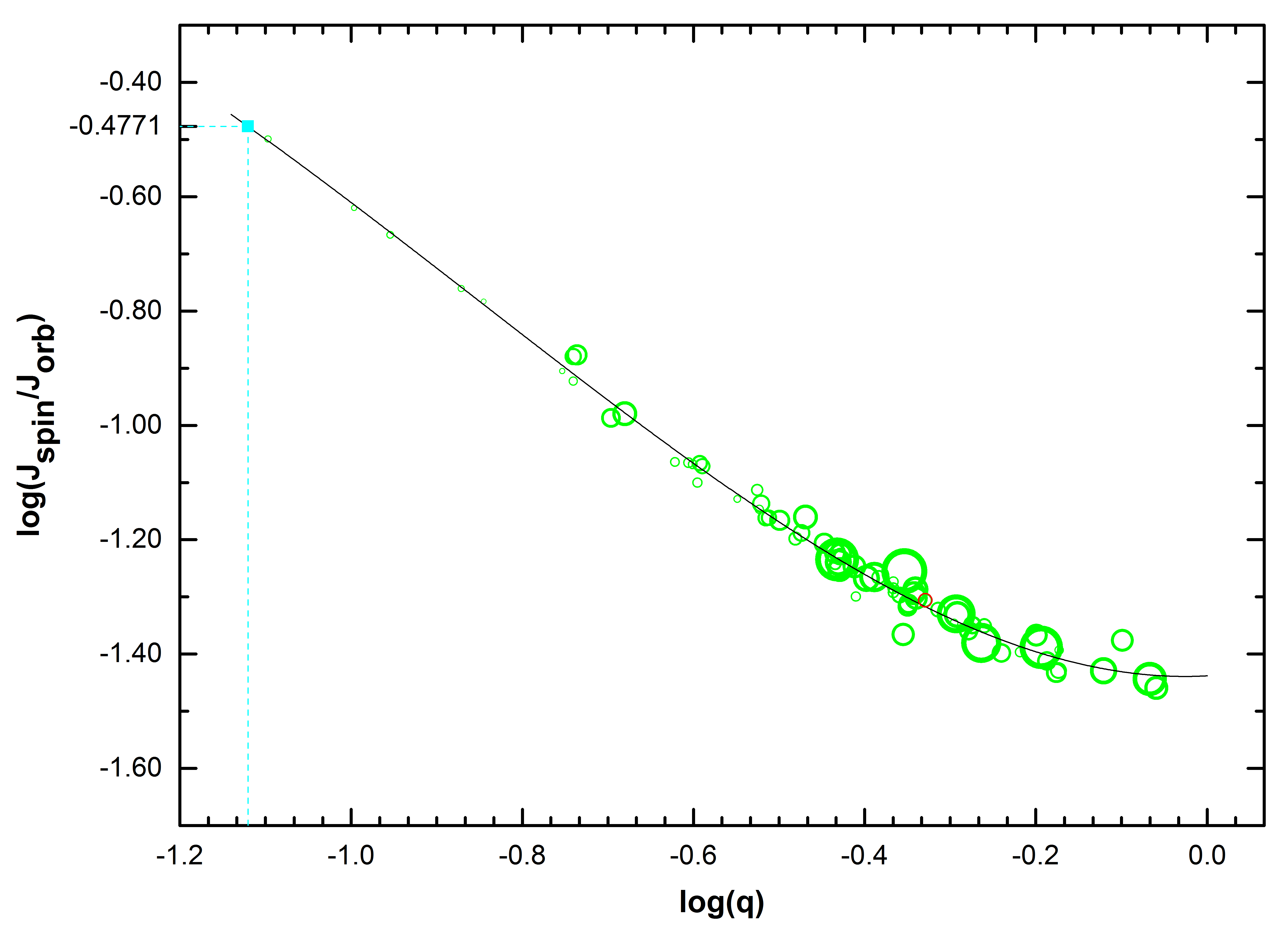
Figure 9: Plots of $log(q)$ - $log(J_{spin}/J_{orb})$ of W-subtype contact binaries. The least-square fitting line is a solid black line. The size of the circle corresponds to the total angular momentum. The cyan square point is the intersection of the black curve with the horizontal line y = log(1/3). BH Cas is signed by the red open circle.

5 Summary

We present the new photometric and optical spectral observations of BH Cas. The O$-$C analysis and the theoretical solution of optical light curves indicate BH Cas to be a W-subtype W UMa contact binary with an orbital period increased with a rate of $\textit{dP/dt}\,=\,+3.27\times 10^{-7}\textrm{d}\,\textrm{yr}^{-1}$. The change of the orbital period may be caused by the mass transfer from $M_{2}$ to $M_{1}$. One cyclical oscillation ($A^{\prime}=0.00300$ days and $P^{\prime}=20.09$ yrs) superimposed on the long-term period increasing tendency, which we attribute to a additional components in the system, e.g., a low-mass star. In the multi-band optical light curves, the strong spot activities and the optical flare are detected at the same time on a W UMa-type system for the first time. Solutions using the W-D code suggest the existence of a cool spot on the secondary star. The spectra observed at phases $\sim$0.0 and $\sim 0.5$ in 2018 and 2019 led to spectral typing of K3V$\pm 1$ and G8V$\pm 2$, respectively. The primary star likely has a spectral type of K3V$\pm 1$. The absolute parameters of BH Cas are obtained, including the mass, radius, and surface gravity, etc. The X-ray data extracted from the XMM-Newton show a light curve with no evidence of occultation as seen in the optical, and X-ray spectra consistent with black-body or bremsstrahlung thermal emission.

6 Acknowledgements

We thank the anonymous referee very much for his/her constructive suggestions, which helped to improve the paper a lot. We acknowledge the support of the staff of the Xinglong 2.16m telescope. This work was partially supported by the Open Project of the Key Laboratory of Optical Astronomy, National Astronomical Observatories, Chinese Academy of Science. We also acknowledge the support of X-ray data based on observations obtained with XMM-Newton, an ESA science mission with instruments and contributions directly funded by ESA Member States and NASA. This research is supported by the National Natural Science Foundation of China (grant Nos.11873081, 11661161016), the program of the light in Chinese Western Region (LCWR; grant Nos.2015-XBQN-A-02),2017 Heaven Lake Hundred-Talent Program of Xinjiang Uygur Autonomous Region of China, the Youth Innovation Promotion Association CAS (grant Nos.2018080). We thanks to Prof. Wenping Chen and Weiyang Wang, for their comments on this paper.

Appendix A BASIC Parameters of W UMa type and Near-contact binaries

Table 10: Fundamental properties of W-subtype W UMa type binaries. Columns are organized as name, subtype, period, radii of primary and secondary, primary and secondary masses, the ratio of spin specific angular momentum to orbital specific angular momentum, the sum of spin specific angular momentum to orbital specific angular momentum and the numbers for references.

Name	Subtype	Period	R1	R2	M1	M2	Jspin/Jorb	Jspin+Jorb	Ref
		d	(R⊙)	(R⊙)	(M⊙)	(M⊙)
GSC 03122-02426	W	0.30	1.30	0.83	2.19	0.81	0.058	97.046	44
DN Cam	W	0.50	1.78	1.22	1.85	0.82	0.056	101.841	1,41
ER Ori	W	0.42	1.39	1.14	1.53	0.98	0.041	95.960	5,35
EF Boo	W	0.43	1.46	1.09	1.61	0.82	0.047	86.367	35,41
AA UMa	W	0.47	1.47	1.11	1.56	0.85	0.042	89.033	35,41
BI Cvn	W	0.38	1.37	0.92	1.59	0.65	0.054	67.387	28
RR Cen	W	0.61	2.10	1.05	1.82	0.38	0.105	55.342	37
YY Eri	W	0.32	1.20	0.77	1.55	0.62	0.054	59.627	7,41
FZ Ori	W	0.39	1.16	1.082	1.17	1.00	0.036	76.048	23
ET Leo	W	0.35	1.36	0.84	1.59	0.54	0.069	55.806	4,41
V502 Oph	W	0.45	1.51	0.93	1.51	0.56	0.058	59.990	7,41
W UMa	W	0.33	1.17	0.85	1.35	0.69	0.0467	59.373	7
AE Phe	W	0.36	1.29	0.81	1.38	0.63	0.052	57.474	7
UX Eri	W	0.45	1.45	0.91	1.45	0.54	0.056	55.873	27
V402 Aur	W	0.60	1.98	0.92	1.64	0.33	0.103	44.808	35,46
TY Pup	W	0.82	2.64	1.37	1.65	0.30	0.133	47.196	31
AW Vir	W	0.35	1.08	0.95	1.11	0.84	0.037	60.954	26
V728 Her	W	0.47	1.81	0.92	1.65	0.3	0.132	38.843	35
BB Peg	W	0.36	1.29	0.83	1.42	0.53	0.060	50.613	11
V417 Aql	W	0.37	1.31	0.84	1.40	0.50	0.062	47.971	35,41
AM Leo	W	0.37	1.23	0.85	1.29	0.59	0.045	51.551	41,47
VY Sex	W	0.44	1.50	0.86	1.42	0.45	0.068	47.013	4,41
UV Lyn	W	0.42	1.39	0.89	1.36	0.5	0.060	48.656	34,35
V781 Tau	W	0.41	1.21	0.85	1.29	0.57	0.043	51.488	10,36
IK Boo	W	0.30	0.91	0.85	0.99	0.86	0.035	53.483	14
CW Cas	W	0.32	1.09	0.75	1.25	0.56	0.049	45.809	9
RZ Com	W	0.34	1.12	0.78	1.23	0.55	0.048	45.413	7,41
AH Vir	W	0.41	1.41	0.84	1.36	0.41	0.073	40.798	35
SW Lac	W	0.32	1.03	0.94	0.98	0.78	0.042	50.284	35,41
QW Gem	W	0.36	1.26	0.75	1.31	0.44	0.065	40.256	15,35
EM Lac	W	0.39	1.19	0.97	1.06	0.67	0.043	50.143	26
EZ Hya	W	0.45	1.54	0.85	1.37	0.35	0.086	37.070	35
V842 Her	W	0.42	1.46	0.81	1.36	0.35	0.085	35.970	35
SS Ari	W	0.41	1.36	0.80	1.31	0.40	0.069	38.605	35
GZ And	W	0.31	1.01	0.74	1.12	0.59	0.044	43.216	1,35
V752 Cen	W	0.37	1.28	0.75	1.3	0.4	0.069	37.217	2,35
VY Cet	W	0.34	1.01	0.83	1.02	0.68	0.037	46.856	26
V1139 Cas	W	0.30	0.94	0.76	1.02	0.66	0.039	43.522	17
TW Cet	W	0.32	0.99	0.76	1.06	0.61	0.040	43.019	35,41
V1128 Tau	W	0.31	1.01	0.76	1.09	0.58	0.045	41.729	43
V870 Ara	W	0.40	1.67	0.61	1.5	0.12	0.317	16.553	32,41
AO Cam	W	0.33	1.09	0.73	1.12	0.49	0.050	37.837	1,3
CK Boo	W	0.36	1.45	0.59	1.39	0.16	0.215	17.710	40
U Peg	W	0.38	1.22	0.74	1.15	0.38	0.063	32.372	25,35
EP And	W	0.40	1.27	0.82	1.10	0.41	0.059	34.267	19
AB And	W	0.33	1.05	0.76	1.01	0.49	0.048	34.909	8
V1007 Cas	W	0.33	1.16	0.69	1.14	0.34	0.073	28.141	18
BV Dra	W	0.35	1.12	0.76	1.04	0.43	0.054	32.526	12,35
V757 Cen	W	0.34	0.97	0.80	0.88	0.59	0.037	36.905	35
FU Dra	W	0.31	1.12	0.61	1.17	0.29	0.086	24.393	34,35
GW Cep	W	0.32	1.05	0.67	1.06	0.39	0.057	29.363	26
GM Dra	W	0.34	1.25	0.61	1.21	0.22	0.120	20.532	3,41
V1191 Cyg	W	0.31	1.31	0.52	1.29	0.13	0.240	13.984	33
TX Cnc	W	0.39	1.28	0.91	1.32	0.60	0.051	54.093	20
BH Cas	W	0.41	0.85	0.96	0.45	0.47	0.049	33.296	This work
BX Peg	W	0.28	0.97	0.62	1.02	0.38	0.059	26.720	30,41
V789 Her	W	0.32	1.15	0.62	1.13	0.27	0.091	22.648	18
FU Dra	W	0.31	1.10	0.60	1.12	0.28	0.086	22.799	21
V546 And	W	0.38	1.23	0.66	1.08	0.28	0.079	23.469	6
UY UMa	W	0.38	1.40	0.63	1.19	0.16	0.173	16.242	42
TY Boo	W	0.32	1.00	0.69	0.93	0.40	0.052	27.006	29,41
VW Cep	W	0.28	0.91	0.62	0.93	0.40	0.051	25.827	7
AR Boo	W	0.34	1.00	0.65	0.90	0.35	0.050	23.972	16
V829 Her	W	0.36	1.07	0.74	0.86	0.37	0.053	24.723	35,46
XY Leo	W	0.28	0.83	0.66	0.76	0.46	0.040	24.900	32,41
OU Ser	W	0.30	1.09	0.51	1.02	0.18	0.124	14.429	24,35
V345 Gem	W	0.27	1.09	0.49	1.05	0.15	0.165	12.492	38
BW Dra	W	0.29	0.98	0.55	0.92	0.26	0.074	17.958	12,35
LR Cam	W	0.43	1.27	0.73	0.9	0.27	0.071	20.821	39
V523 Cas	W	0.23	0.74	0.55	0.75	0.38	0.045	19.616	43
CC Com	W	0.22	0.71	0.53	0.72	0.38	0.045	18.639	13
RW Dor	W	0.29	0.80	0.67	0.64	0.43	0.040	20.507	35
RW Com	W	0.24	0.71	0.46	0.56	0.20	0.061	8.971	22,35

Note. — The asterisk (*) refers to assumed, fixed values.

References

- Andrae et al. (2018) Andrae, R., Fouesneau, M., Creevey, O., et al. 2018, A&A, 616, A8
- Applegate (1992) Applegate, J. H. 1992, ApJ, 385, 621
- Arbutina (2007) Arbutina, B. 2007, MNRAS, 377, 1635
- Arbutina (2009) Arbutina, B. 2009, MNRAS, 394, 501
- Arranz Heras & Sanchez-Bajo (2009) Arranz Heras, T., & Sanchez-Bajo, F. 2009, The Observatory, 129, 88
- Baran et al. (2004) Baran, A., Zola, S., Rucinski, S. M., et al. 2004, Acta Astron., 54, 195
- Binnendijk (1970) Binnendijk, L. 1970, Vistas in Astronomy, 12, 217
- Brandt et al. (1997) Brandt, W. N., Ward, M. J., Fabian, A. C., & Hodge, P. W. 1997, MNRAS, 291, 709
- Barone et al. (1993) Barone, F., di Fiore, L., Milano, L., & Russo, G. 1993, ApJ, 407, 237
- Beljawsky (1931) Beljawsky, S. 1931, Astronomische Nachrichten, 243, 115
- Chabrier et al. (2000) Chabrier, G., Baraffe, I., Allard, F., & Hauschildt, P. 2000, ApJ, 542, 464
- Chen et al. (2006) Chen, W. P., Sanchawala, K., & Chiu, M. C. 2006, AJ, 131, 990
- Covey et al. (2007) Covey, K. R., Ivezić, Ž., Schlegel, D., et al. 2007, AJ, 134, 2398
- Cox (2000) Cox, A. N. 2000, Allen’s Astrophysical Quantities,
- Fan et al. (2016) Fan, Z., Wang, H., Jiang, X., et al. 2016, PASP, 128, 115005
- Fox-Machado et al. (2018) Fox-Machado, L., Cang, T. Q., Michel, R., Fu, J. N., & Li, C. Q. 2018, PASP, 130, 104201
- Gaia Collaboration (2018) Gaia Collaboration 2018, VizieR Online Data Catalog, 1345,
- Gazeas et al. (2005) Gazeas, K. D., Baran, A., Niarchos, P., et al. 2005, Acta Astron., 55, 123
- Gazeas et al. (2006) Gazeas, K. D., Niarchos, P. G., Zola, S., Kreiner, J. M., & Rucinski, S. M. 2006, Acta Astron., 56, 127
- Gazeas & Niarchos (2006) Gazeas, K. D., & Niarchos, P. G. 2006, MNRAS, 370, L29
- Goecking et al. (1994) Goecking, K.-D., Duerbeck, H. W., Plewa, T., et al. 1994, A&A, 289, 827
- Gondoin (2004) Gondoin, P. 2004, A&A, 415, 1113
- Gürol et al. (2015) Gürol, B., Bradstreet, D. H., & Okan, A. 2015, New A, 36, 100
- Harmanec (1988) Harmanec, P. 1988, Bulletin of the Astronomical Institutes of Czechoslovakia, 39, 329
- Hilditch et al. (1988) Hilditch, R. W., King, D. J., & McFarlane, T. M. 1988, MNRAS, 231, 341
- Hoffman et al. (2006) Hoffman, D. I., Harrison, T. E., McNamara, B. J., et al. 2006, AJ, 132, 2260
- Hrivnak (1988) Hrivnak, B. J. 1988, ApJ, 335, 319
- Hu et al. (2016) Hu, C.-P., Yang, T.-C., Chou, Y., et al. 2016, AJ, 151, 170
- Huenemoerder et al. (2006) Huenemoerder, D. P., Testa, P., & Buzasi, D. L. 2006, ApJ, 650, 1119
- Huruhata (1952) Huruhata, M. 1952, PASP, 64, 200
- Jansen et al. (2001) Jansen, F., Lumb, D., Altieri, B., et al. 2001, A&A, 365, L1
- Jiang et al. (2010) Jiang, T.-Y., Li, L.-F., Han, Z.-W., & Jiang, D.-K. 2010, PASJ, 62, 457
- Kalberla et al. (2005) Kalberla, P. M. W., Burton, W. B., Hartmann, D., et al. 2005, A&A, 440, 775
- Kallrath et al. (2006) Kallrath, J., Milone, E. F., Breinhorst, R. A., et al. 2006, A&A, 452, 959
- Kalomeni et al. (2007) Kalomeni, B., Yakut, K., Keskin, V., et al. 2007, AJ, 134, 642
- Kaluzny & Rucinski (1986) Kaluzny, J., & Rucinski, S. M. 1986, AJ, 92, 666
- Kandulapati et al. (2015) Kandulapati, S., Devarapalli, S. P., & Pasagada, V. R. 2015, MNRAS, 446, 510
- Kesseli et al. (2017) Kesseli, A. Y., West, A. A., Veyette, M., et al. 2017, ApJS, 230, 16
- Kopal (1978) Kopal, Z. 1978, Astrophysics and Space Science Library, 68
- Köse et al. (2011) Köse, O., Kalomeni, B., Keskin, V., Ulaş, B., & Yakut, K. 2011, Astronomische Nachrichten, 332, 626
- Kriwattanawong et al. (2017) Kriwattanawong, W., Sanguansak, N., & Maungkorn, S. 2017, PASJ, 69, 62
- Kreiner et al. (2003) Kreiner, J. M., Rucinski, S. M., Zola, S., et al. 2003, A&A, 412, 465
- Kukarkin (1938) Kukarkin,B. 1938, Veranderl.Sterne Nishni-Novgorod, 5,195
- Lanza & Rodonò (2002) Lanza, A. F., & Rodonò, M. 2002, Astronomische Nachrichten, 323, 424
- Lee et al. (2008) Lee, J. W., Youn, J.-H., Kim, C.-H., Lee, C.-U., & Kim, H.-I. 2008, AJ, 135, 1523
- Lee et al. (2009) Lee, J. W., Youn, J.-H., Lee, C.-U., Kim, S.-L., & Koch, R. H. 2009, AJ, 138, 478
- Li et al. (2004) Li, L., Han, Z., & Zhang, F. 2004, MNRAS, 351, 137
- Li et al. (2015) Li, K., Hu, S.-M., Guo, D.-F., et al. 2015, New A, 34, 217
- Li et al. (2018) Li, K., Xia, Q.-Q., Hu, S.-M., Guo, D.-F., & Chen, X. 2018, PASP, 130, 074201
- Li & Zhang (2006) Li, L., & Zhang, F. 2006, MNRAS, 369, 2001
- Liao et al. (2013) Liao, W.-P., Qian, S.-B., Li, K., et al. 2013, AJ, 146, 79
- Liu et al. (2007) Liu, L., Qian, S.-B., Boonrucksar, S., et al. 2007, PASJ, 59, 607
- Liu et al. (2012) Liu, L., Qian, S.-B., He, J.-J., et al. 2012, PASJ, 64, 48
- Lu & Rucinski (1999) Lu, W., & Rucinski, S. M. 1999, AJ, 118, 515
- Lucy (1967) Lucy, L. B. 1967, ZAp, 65, 89
- Ma et al. (2018) Ma, S.-G., Esamdin, A., Ma, L., et al. 2018, Ap&SS, 363, 68
- Mallik (1997) Mallik, S. V. 1997, A&AS, 124, 359
- McCartney (1997) McCartney, S. 1997, The Third Pacific Rim Conference on Recent Development on Binary Star Research, 130, 129
- Milone et al. (1987) Milone, E. F., Wilson, R. E., & Hrivnak, B. J. 1987, ApJ, 319, 325
- Metcalfe (1999) Metcalfe, T. S. 1999, AJ, 117, 2503
- Milone (1968) Milone, E. E. 1968, AJ, 73, 708
- Molík (1998) Molík, P. 1998, 20th Stellar Conference of the Czech and Slovak Astronomical Institutes, 81
- Müller (1903) Müller, G. 1903, Popular Astronomy, 11, 138
- Niarchos et al. (2001) Niarchos, P. G., Aslanidis, D., Zola, S., & Theodossiou, E. 2001, 5th Hellenic Astronomical Conference, 77.1
- Nef & Rucinski (2008) Nef, P. D., & Rucinski, S. M. 2008, MNRAS, 385, 2239
- O’Connell (1951) O’Connell, D. J. K. 1951, Publications of the Riverview College Observatory, 2, 85
- Pasham et al. (2013) Pasham, D. R., Strohmayer, T. E., & Mushotzky, R. F. 2013, ApJ, 771, L44
- Pi et al. (2017) Pi, Q.-f., Zhang, L.-y., Bi, S.-l., et al. 2017, AJ, 154, 260
- Prasad et al. (2014) Prasad, V., Pandey, J. C., Patel, M. K., & Srivastava, D. C. 2014, Ap&SS, 353, 575
- Pribulla et al. (1999) Pribulla, T., Chochol, D., Rovithis-Livaniou, H., & Rovithis, P. 1999, A&A, 345, 137
- Pribulla & Vanko (2002) Pribulla, T., & Vanko, M. 2002, Contributions of the Astronomical Observatory Skalnate Pleso, 32, 79
- Prša & Zwitter (2005) Prša, A., & Zwitter, T. 2005, ApJ, 628, 426
- Shengbang & Qingyao (2000) Shengbang, Q., & Qingyao, L. 2000, Ap&SS, 271, 331
- Qian (2001) Qian, S. 2001, MNRAS, 328, 635
- Qian (2003) Qian, S. 2003, MNRAS, 342, 1260
- Qian et al. (2007) Qian, S.-B., Yuan, J.-Z., Xiang, F.-Y., et al. 2007, AJ, 134, 1769
- Qian et al. (2008) Qian, S.-B., He, J.-J., Liu, L., Zhu, L.-Y., & Liao, W. P. 2008, AJ, 136, 2493
- Qian et al. (2012) Qian, S.-B., Zhang, J., Zhu, L.-Y., et al. 2012, MNRAS, 423, 3646
- Qian et al. (2014) Qian, S.-B., Wang, J.-J., Zhu, L.-Y., et al. 2014, ApJS, 212, 4
- Rainger et al. (1990) Rainger, P. P., Hilditch, R. W., & Bell, S. A. 1990, MNRAS, 246, 42
- Riaz et al. (2018) Riaz, R., Vanaverbeke, S., & Schleicher, D. R. G. 2018, MNRAS, 478, 5460
- Rovithis-Livaniou et al. (2000) Rovithis-Livaniou, H., Kranidiotis, A. N., Rovithis, P., & Athanassiades, G. 2000, A&A, 354, 904
- Ruciński (1969) Ruciński, S. M. 1969, Acta Astron., 19, 245
- Samec & Hube (1991) Samec, R. G., & Hube, D. P. 1991, AJ, 102, 1171
- Sarotsakulchai et al. (2018) Sarotsakulchai, T., Qian, S.-B., Soonthornthum, B., et al. 2018, AJ, 156, 199
- Shapley (1948) Shapley, H. 1948, Harvard Observatory Monographs, 7, 249
- Song et al. (2016) Song, F.-F., Esamdin, A., Ma, L., et al. 2016, Research in Astronomy and Astrophysics, 16, 154
- Stȩpień et al. (2001) Stȩpień, K., Schmitt, J. H. M. M., & Voges, W. 2001, A&A, 370, 157
- Stone (1974) Stone, R. P. S. 1974, ApJ, 193, 135
- Strüder et al. (2001) Strüder, L., Briel, U., Dennerl, K., et al. 2001, A&A, 365, L18
- Szalai et al. (2007) Szalai, T., Kiss, L. L., Mészáros, S., Vinkó, J., & Csizmadia, S. 2007, A&A, 465, 943
- Tout & Hall (1991) Tout, C. A., & Hall, D. S. 1991, MNRAS, 253, 9
- Turner et al. (2001) Turner, M. J. L., Abbey, A., Arnaud, M., et al. 2001, A&A, 365, L27
- Ulaş et al. (2012) Ulaş, B., Kalomeni, B., Keskin, V., Köse, O., & Yakut, K. 2012, New A, 17, 46
- van Hamme (1993) van Hamme, W. 1993, AJ, 106, 2096
- Vanko et al. (2001) Vanko, M., Pribulla, T., Chochol, D., et al. 2001, Contributions of the Astronomical Observatory Skalnate Pleso, 31, 129
- Vilhu & Maceroni (2007) Vilhu, O., & Maceroni, C. 2007, Binary Stars as Critical Tools Tests in Contemporary Astrophysics, 240, Harmanec
- Wilson & Devinney (1971) Wilson, R. E., & Devinney, E. J. 1971, ApJ, 166, 605
- Wilson (1979) Wilson, R. E. 1979, ApJ, 234, 1054
- Wilson (2012) Wilson, R. E. 2012, AJ, 144, 73
- Yakut & Eggleton (2005) Yakut, K., & Eggleton, P. P. 2005, ApJ, 629, 1055
- Yakut et al. (2005) Yakut, K., Ulaş, B., Kalomeni, B., & Gülmen, Ö. 2005, MNRAS, 363, 1272
- Yang et al. (2005) Yang, Y.-G., Qian, S.-B., Zhu, L.-Y., He, J.-J., & Yuan, J.-Z. 2005, PASJ, 57, 983
- Yang et al. (2009) Yang, Y.-G., Qian, S.-B., Zhu, L.-Y., & He, J.-J. 2009, AJ, 138, 540
- Yang & Dai (2010) Yang, Y.-G., & Dai, H.-F. 2010, PASJ, 62, 1045
- Yang et al. (2012) Yang, Y.-G., Qian, S.-B., & Soonthornthum, B. 2012, AJ, 143, 122
- Yildiz & Doğan (2013) Yildiz, M., & Doğan, T. 2013, MNRAS, 430, 2029
- Yu et al. (2017) Yu, Y.-X., Zhang, X.-D., Hu, K., & Xiang, F.-Y. 2017, New A, 55, 13
- Zhang & Zhang (2004) Zhang, X. B., & Zhang, R. X. 2004, MNRAS, 347, 307
- Zhang et al. (2011) Zhang, X.-B., Ren, A.-B., Luo, C.-Q., & Luo, Y.-P. 2011, Research in Astronomy and Astrophysics, 11, 583
- Zhou et al. (2016) Zhou, X., Qian, S.-B., He, J.-J., Zhang, J., & Zhang, B. 2016, New A, 48, 12
- Zoła et al. (2001) Zoła, S., Niarchos, P., Manimanis, V., & Dapergolas, A. 2001, A&A, 374, 164
- Zola et al. (2004) Zola, S., Rucinski, S. M., Baran, A., et al. 2004, Acta Astron., 54, 299
- Zola et al. (2010) Zola, S., Gazeas, K., Kreiner, J. M., et al. 2010, MNRAS, 408, 464