Efficient high order accurate staggered semi-implicit discontinuous Galerkin methods for natural convection problems

Abstract

In this article we propose a new family of high order staggered semi-implicit discontinuous Galerkin (DG) methods for the simulation of natural convection problems. Assuming small temperature fluctuations, the Boussinesq approximation is valid and in this case the flow can simply be modeled by the incompressible Navier-Stokes equations coupled with a transport equation for the temperature and a buoyancy source term in the momentum equation. Our numerical scheme is developed starting from the work presented in [1, 2, 3], in which the spatial domain is discretized using a face-based staggered unstructured mesh. The pressure and temperature variables are defined on the primal simplex elements, while the velocity is assigned to the dual grid. For the computation of the advection and diffusion terms, two different algorithms are presented: i) a purely Eulerian upwind-type scheme and ii) an Eulerian-Lagrangian approach. The first methodology leads to a conservative scheme whose major drawback is the time step restriction imposed by the CFL stability condition due to the explicit discretization of the convective terms. On the contrary, computational efficiency can be notably improved relying on an Eulerian-Lagrangian approach in which the Lagrangian trajectories of the flow are tracked back. This method leads to an unconditionally stable scheme if the diffusive terms are discretized implicitly. Once the advection and diffusion contributions have been computed, the pressure Poisson equation is solved and the velocity is updated. As a second model for the computation of buoyancy-driven flows, in this paper we also consider the full compressible Navier-Stokes equations. The staggered semi-implicit DG method first proposed in [4] for all Mach number flows is properly extended to account for the gravity source terms arising in the momentum and energy conservation laws. In order to assess the validity and the robustness of our novel class of staggered semi-implicit DG schemes, several classical benchmark problems are considered, showing in all cases a good agreement with available numerical reference data. Furthermore, a detailed comparison between the incompressible and the compressible solver is presented. Finally, advantages and disadvantages of the Eulerian and the Eulerian-Lagrangian methods for the discretization of the nonlinear convective terms are carefully studied.

1 Introduction

Natural convection problems play an important role in computational fluid dynamics. They appear in numerous engineering applications and natural phenomena ranging from the design of cooling devices in industrial processes, electronics, building isolation or solar energy collectors, to the simulation of atmospheric flows. In the last decades, the scientific community has put a lot of efforts into the study of these phenomena, see e.g. [5, 6, 7, 8, 9, 10] for a non-exhaustive overview. Nowadays, the main challenge is to develop efficient high order numerical methods which are able to capture even small scale structures of the flow, avoiding the use of RANS turbulence models (see [11, 12]). In this paper, we propose a novel family of high order accurate staggered semi-implicit discontinuous Galerkin (DG) methods, which extends the works presented in [1, 3, 4] appropriately to deal also with gravity driven flows.

Depending on the magnitude of the temperature perturbation and on the importance of density changes, natural convection problems are usually divided into two main groups. If the Mach number and the temperature fluctuations are small, the incompressible Navier-Stokes equations under the usual Boussinesq assumption can be applied. Otherwise, the full compressible Navier-Stokes equations have to be employed. In the following, we will mainly focus on the first case. However, in this paper also the compressible model will be considered, thus allowing for a direct comparison of the results obtained using the two different systems of governing partial differential equations. Therefore, we will be able to further validate the applicability of the Boussinesq approach for the flow regimes we are interested in.

In the literature there are numerous approaches that have been proposed for the solution of the Navier-Stokes equations, such as finite difference methods [13, 14, 15, 16] or continuous finite element schemes [17, 18, 19, 20, 21, 22, 23]. Nevertheless, the construction of high order numerical methods, and especially of high order discontinuous Galerkin (DG) finite element schemes, is still a very active research field, which has started with the pioneering works of Bassi and Rebay [24], and Baumann and Oden [25, 26]. Later, several high order DG methods for the incompressible and compressible Navier-Stokes equations have been proposed, see for example [27, 28, 29, 30, 31, 32, 33, 34, 35, 36, 37, 38, 39]. We also would like to mention recent works on semi-implicit DG schemes that can be found in [40, 41, 42, 43, 44], to which our approach is indirectly related.

The algorithm proposed in this article makes use of the novel family of staggered semi-implicit DG schemes that has been introduced in [1, 2, 3] for the incompressible Navier-Stokes equations in two and three space dimensions and which was later also extended to the full compressible regime in [4], following the work outlined in [45, 46, 47]. These arbitrary high order accurate DG schemes are constructed on staggered unstructured meshes. The pressure, the density and the energy are defined on the triangular or tetrahedral primal grid, whereas the velocity is computed on a face-based staggered dual mesh. While the use of staggered grids is a very common practice in the finite difference and finite volume framework (see e.g. [13, 14, 48]), its use is not so widespread in the context of high order DG schemes. The first staggered DG methods, which adopted a vertex-based dual grid, have been proposed in [49, 50]. Other recent high order staggered DG algorithms that rely on an edge-based dual grid have been advanced in [51, 52]. For high order staggered semi-implicit discontinuous Galerkin schemes on uniform and adaptive Cartesian meshes, see [53, 54].

Focusing on the incompressible model, we propose two different approaches for the computation of the nonlinear convective terms. On the one hand, we consider the methodology already introduced in [3]. There, the convective subsystem for the velocity is solved considering the Rusanov flux function for an explicit upwind-type discretization of the nonlinear convective terms. Instead, the viscous terms are discretized implicitly, making again use of the dual mesh in order to obtain the discrete gradients, without needing any additional numerical flux function for the viscous terms. One of the major drawbacks of this approach is its high computational cost coming from the small time step dictated by the CFL stability condition due to the explicit discretization of the convective terms. Moreover, to avoid spurious oscillations, a limiter should be used (see [4]). As an alternative option, which is at the same time able to deal with large gradients and substantially reduces the computational cost, we propose the use of an Eulerian-Lagrangian approach, recently forwarded in [55] also in the context of high order in space staggered DG schemes. The trajectory of the flow particles is followed backward in time by integrating the associated trajectory equations at the aid of a high order Taylor series expansion, where time derivatives are replaced by spatial derivatives using the Cauchy-Kovalevskaya procedure, similar to the ADER approach of Toro and Titarev [56, 57, 58]. The high order spatial discretization of the DG scheme is then employed to obtain a high order time integration for each point needed to solve numerically the advection part of the governing equations. For further information on efficient semi-Lagrangian and Eulerian-Lagrangian schemes we refer the reader to [59, 60, 61, 62, 63, 64, 65, 66, 67, 68, 69].

The use of the Boussinesq assumption yields the coupling of the incompressible Navier-Stokes equations with an additional conservation equation for the temperature. The computation of the related advection and diffusion terms is performed similarly to what is done for the velocity in the momentum equation. Nevertheless, let us remark that the temperature is defined on the primal mesh so that interpolation from one mesh to the other is avoided in the fully Eulerian approach. Once the new temperature is known, the gravity source term in the momentum equation can be evaluated. Finally, the pressure Poisson equation is solved and the velocity at the new time step is computed.

Regarding the compressible Navier-Stokes equations, we extend the numerical scheme introduced in [4] to consider the additional gravity terms. To this end, two new terms are included in the pressure system which has been obtained by formal substitution of the discrete momentum equation into the discrete energy equation. The first gravity term, coming from the momentum equation, is computed jointly with the convective and viscous terms of the momentum equation at the beginning of each time step. Meanwhile, the gravity term embedded in the energy equation is computed at each Picard iteration using the updated values of the linear momentum density.

The rest of the paper is organized as follows. In Section 2 we recall the incompressible and compressible Navier-Stokes equations. For the incompressible model, the Boussinesq assumption is made to account for fluid flow with small temperature variations under gravity effects. Concerning the compressible model, we consider the full Navier-Stokes equations including the conservation law for the total energy density and assuming here the equation of state for an ideal gas. Section 3 is devoted to the description of the semi-implicit staggered DG method used to solve the incompressible model in two and three space dimensions. We start by recalling some basic definitions about the usage of staggered meshes and the polynomial spaces which are employed. Next, we derive the numerical method considering two different frameworks for the discretization of convective and diffusive terms, namely an Eulerian and an Eulerian-Lagrangian approach. The extension of the algorithm to the compressible case is described in Section 4. Several benchmarks are presented in Section 6, aiming at assessing the validity, efficiency and the robustness of our novel numerical schemes. The main pros and cons of the Eulerian and the Eulerian-Lagrangian approaches are analyzed as well. Finally, we compare the results obtained with the incompressible solver against those computed with the compressible solver in the low Mach number regime.

2 Governing equations

As already mentioned, natural convection problems may be studied using two different models: the incompressible and the compressible Navier-Stokes equations, both including proper gravitational terms. The choice of the model usually depends on specific features of the flow under consideration, like the magnitude of the temperature fluctuations or the importance of capturing density variations. Here, we are mainly interested in small temperature changes, so that we will firt focus on the incompressible case. Later, even the full compressible model will be studied and numerical results will be compared considering both approaches.

2.1 Incompressible Navier-Stokes equations

Let us consider the laminar flow of a single phase Newtonian fluid without neither radiation nor chemical reactions. Let furthermore $\beta$ be the thermal expansion coefficient of the fluid, $\theta_{0}$ the reference temperature of the flow and $\theta_{\mathrm{b}}-\theta_{0}$ the maximum temperature fluctuation. Under the assumption

$$\beta(\theta_{\mathrm{b}}-\theta_{0})\ll 1,$$ (1)

the Boussinesq approximation for buoyancy-driven flows holds. Therefore, natural convection problems with small temperature gradients may be analyzed by solving the system of incompressible Navier-Stokes equations coupled with an energy conservation equation through an additional source term in the momentum equation. The governing PDE system reads as follows:

$$\nabla\cdot\mathbf{v}=0,$$ (2)

$$\frac{\partial\mathbf{v}}{\partial t}+\nabla\cdot\mathbf{F}^{\mathbf{v}}_{c}+\nabla p=\nabla\cdot\left(\nu\nabla\mathbf{v}\right)+\left(1-\beta\delta\theta\right)\mathbf{g},$$ (3)

$$\frac{\partial{\theta}}{\partial{t}}+\nabla\cdot\mathbf{F}^{\theta}_{c}=\nabla\cdot\left(\alpha\nabla\theta\right),$$ (4)

where $\mathbf{v}$ is the velocity field; $p=P/\rho$ indicates the normalized fluid pressure; $P$ is the physical pressure and $\rho$ is the fluid density, which according to the Boussinesq approximation is assumed to be constant everywhere apart from the gravity source term in the momentum equation; $\nu=\mu/\rho$ is the kinematic viscosity coefficient; $\mathbf{F}^{\mathbf{v}}_{c}=\mathbf{v}\otimes\mathbf{v}$ is the flux tensor of the nonlinear convective terms; $\delta\theta:=\theta-\theta_{0}$ is the temperature difference; $\mathbf{g}$ is the gravity acceleration; $\theta$ is the temperature; $\mathbf{F}_{c}^{\theta}=\mathbf{v}\theta$ is the flux tensor of the nonlinear convective terms of the energy equation; $\alpha=\kappa/(\rho c_{P})$ is the thermal diffusivity, which depends on the thermal conductivity $\kappa$, the density $\rho$ and the heat capacity $c_{P}$. Let us also introduce the following notation:

$$\mathbf{F}^{\mathbf{v}}:=\mathbf{F}_{c}^{\mathbf{v}}-\nu\nabla\mathbf{v},\qquad\mathbf{L}^{\mathbf{v}}\left(\mathbf{v}\right):=\frac{\partial}{\partial t}\mathbf{v}+\nabla\cdot\mathbf{F}^{\mathbf{v}},$$ (5)

$$\mathbf{F}^{\theta}:=\mathbf{F}^{\theta}_{c}-\nabla\cdot\alpha\nabla\theta,\qquad\mathbf{L}^{\theta}\left(\theta,\mathbf{v}\right):=\frac{\partial}{\partial t}\theta+\nabla\cdot\mathbf{F}^{\theta}.$$ (6)

2.2 Compressible Navier-Stokes equations

Large temperature fluctuations may produce substantial changes in the density of a fluid. As a consequence, the incompressible model (2)-(4) is no longer valid for large temperature fluctuations. In this case, one must use the full compressible Navier-Stokes equations under gravitational effects, that read

$$\frac{\partial\rho}{\partial t}+\nabla\cdot\left(\rho\mathbf{v}\right)=0,$$ (7)

$$\frac{\partial\rho\mathbf{v}}{\partial t}+\nabla\cdot\mathbf{F}^{\rho\mathbf{v}}_{c}+\nabla P=\nabla\cdot\bm{\sigma}+\rho\mathbf{g},$$ (8)

$$\frac{\partial{\rho E}}{\partial{t}}+\nabla\cdot\mathbf{F}^{\rho E}_{c}=\nabla\cdot\left(\bm{\sigma}\mathbf{v}+\kappa\nabla\theta\right)+\rho\mathbf{g}\cdot\mathbf{v},$$ (9)

where $\mathbf{F}^{\rho\mathbf{v}}_{c}=\rho\mathbf{v}\otimes\mathbf{v}$ is the convective flux for the momentum equation; $\bm{\sigma}=\mu(\nabla{\mathbf{v}}+\nabla{\mathbf{v}}^{\top})-\frac{2}{3}\mu\left(\nabla\cdot{\mathbf{v}}\right)\mathbf{I}$ is the viscous stress tensor; $\rho E=\rho{e}+\rho{k}$ is the total energy density; $\rho{k}=\frac{1}{2}\rho{\mathbf{v}}^{2}$ is the kinetic energy density; $e=e(P,\rho)$ represents the specific internal energy per unit mass and is given by the equation of state (EOS) as a function of the pressure $P$ and the density $\rho$; $H=e+\frac{P}{\rho}$ denotes the specific enthalpy; $\mathbf{F}^{\rho E}_{c}=\mathbf{v}\left(\rho E+P\right)=\rho\mathbf{v}k+\rho\mathbf{v}H$ is the convective flux for the energy conservation equation; $\kappa$ is the thermal conductivity coefficient. Let us also define the following operators:

$$\mathbf{F}^{\rho\mathbf{v}}:=\mathbf{F}^{\rho\mathbf{v}}_{c}-\bm{\sigma},\qquad\mathbf{L}^{\rho\mathbf{v}}\left(\rho\mathbf{v}\right):=\frac{\partial}{\partial t}\mathbf{v}+\nabla\cdot\mathbf{F}^{\rho\mathbf{v}}.$$ (10)

In our approach we assume that we are dealing with an ideal gas, so that the thermal and caloric equation of state (EOS) that are needed to close the above system are given by

$$P=\rho R\theta,\qquad e=c_{v}\theta,\qquad\textnormal{hence}\qquad P=(\gamma-1)\rho e,$$ (11)

with $R=c_{P}+c_{v}$ denoting the specific gas constant; $c_{P}$ and $c_{v}$ representing the heat capacities at constant pressure and at constant volume, respectively, and $\gamma=c_{P}/c_{v}$ being the usual ratio of specific heats.

3 Numerical method for the incompressible model

System (2)-(4) will be solved starting by the staggered semi-implicit discontinuous Galerkin scheme detailed in [1, 2, 3]. Here, we recall the main ingredients of the algorithm, while for an exhaustive description the reader is referred to the aforementioned references.

3.1 Staggered unstructured mesh

The computational domain is discretized using a face-based staggered unstructured meshes, as adopted in [1, 2, 3, 4]. In what follows, we briefly summarize the grid construction and the main notation for the two dimensional triangular grid. After that, the primal and dual spatial elements are extended to the three dimensional case.

The spatial computational domain $\Omega\subset\mathbb{R}^{2}$ is covered with a set of $N_{e}$ non-overlapping triangular elements $\mathbf{T}_{i}$ with $i=1\ldots N_{e}$. By denoting with $N_{d}$ the total number of edges, the $j-$th edge will be called $\Gamma_{j}$. $\mathcal{B}(\Omega)$ refers to the set of indices $j$ corresponding to boundary edges. The three edges of each triangle $\mathbf{T}_{i}$ constitute the set $S_{i}$ defined by $S_{i}=\{j\in[1,N_{d}]\,\,|\,\,\Gamma_{j}\mbox{ is an edge of }\mathbf{T}_{i}\}$. For every $j\in[1\ldots N_{d}]-\mathcal{B}(\Omega)$ there exist two triangles $i_{1}$ and $i_{2}$ that share $\Gamma_{j}$. We assign arbitrarily a left and a right triangle called $\ell(j)$ and $r(j)$, respectively. The standard positive direction is assumed to be from left to right. Let $\vec{n}_{j}$ denote the unit normal vector defined on the edge $j$ and oriented with respect to the positive direction. For every triangular element $i$ and edge $j\in S_{i}$, the neighbor triangle of element $\mathbf{T}_{i}$ that share the edge $\Gamma_{j}$ is denoted by $\mathbb{\wp}(i,j)$.

For every $j\in[1,N_{d}]-\mathcal{B}(\Omega)$ the quadrilateral element associated to $j$ is called $\mathbf{R}_{j}$ and it is defined, in general, by the two centers of gravity of $\ell(j)$ and $r(j)$ and the two terminal nodes of $\Gamma_{j}$, see also [70, 71, 72, 52]. We denote by $\mathbf{T}_{i,j}=\mathbf{R}_{j}\cap\mathbf{T}_{i}$ the intersection element for every $i$ and $j\in S_{i}$. Figure 1 summarizes the notation, the primal triangular mesh and the dual quadrilateral grid.

Figure 1: Triangular mesh element with its three neighbors and the associated staggered edge-based dual control volumes, together with the notation used throughout the paper.

According to [2], we will call the main grid, or primal grid, the mesh of triangular elements $\{\mathbf{T}_{i}\}_{i\in[1,N_{e}]}$, whereas the quadrilateral grid $\{\mathbf{R}_{j}\}_{j\in[1,N_{d}]}$ is addressed as the dual grid.

The definitions given above are then readily extended to three space dimensions within a domain $\Omega\subset\mathbb{R}^{3}$.

Figure 2: Tetrahedral element of the primary mesh with $S_{i}=\{j_{1},j_{2},j_{3},j_{4}\}$ (left) and non-standard dual face-based hexahedral element associated to the face $j_{3}$ (right).

An example of the resulting main and dual grids in three space dimensions is reported in Figure 2. The main grid consists of tetrahedral simplex elements, and the face-based dual elements contain the three vertices of the common triangular face of two tetrahedra (a left and a right one), and the two barycenters of the two tetrahedra that share the same face. Therefore, in three space dimensions the dual grid consists of non-standard five-point hexahedral elements. The same face-based staggered dual mesh has also been used in [71, 73, 74, 75].

3.2 Basis functions

The basis functions are chosen according to [1, 3], thus, in the two dimensional case we first construct the polynomial basis up to a generic polynomial of degree $p$ on some triangular and quadrilateral reference elements with local coordinates $\xi$ and $\eta$. The reference triangle is considered to be $T_{std}=\{(\xi,\eta)\in\mathbb{R}^{2}\,\,|\,\,0\leq\xi\leq 1,\,\,0\leq\eta\leq 1-\xi\}$ and the reference quadrilateral element is defined as $R_{std}=[0,1]^{2}$. Then, the standard nodal approach of conforming continuous finite elements yields $N_{\phi}=\frac{(p+1)(p+2)}{2}$ basis functions denoted with $\{\phi_{k}\}_{k\in[1,N_{\phi}]}$ on $T_{std}$, and $N_{\psi}=(p+1)^{2}$ basis functions referred to as $\{\psi_{k}\}_{k\in[1,N_{\psi}]}$ on $R_{std}$. The transformation between the reference coordinates $\bm{\xi}=(\xi,\eta)$ and the physical coordinates $\mathbf{x}=(x,y)$ is performed by the maps $T_{i}:\mathbf{T}_{i}\longrightarrow T_{std}$ for every $i=1\ldots N_{e}$ and $T_{j}:\mathbf{R}_{j}\longrightarrow R_{std}$ for every $j=1\ldots N_{d}$, with the associated inverse relations, namely $T_{i}^{-1}:\mathbf{T}_{i}\longleftarrow T_{std}$ and $T_{j}^{-1}:\mathbf{R}_{j}\longleftarrow R_{std}$, respectively.

For the three-dimensional tetrahedra, we use again the standard nodal basis functions of conforming finite elements based on the reference element $T_{std}=\{(\xi,\eta,\zeta)\in\mathbb{R}^{3}\,\,|\,\,0\leq\xi\leq 1,\,\,0\leq\eta\leq 1-\xi,\,\,0\leq\zeta\leq 1-\xi-\eta\}$ and then we define a map to connect the reference space, $\bm{\xi}=(\xi,\eta,\zeta)$, to the physical space, $\mathbf{x}=(x,y,z)$, and vice-versa. Unfortunately, the non-standard five-point hexahedral elements of the dual mesh entail the definition of a polynomial basis directly in the physical space using a simple modal basis based on rescaled Taylor monomials, such as the ones proposed in [3]. We thus obtain $N_{\phi}=N_{\psi}=\frac{1}{6}(p+1)(p+2)(p+3)$ basis functions per element for both the main grid and the dual mesh.

3.3 Staggered semi-implicit DG scheme

The discrete pressure and temperature are defined on the main grid, that is $p_{i}(\mathbf{x},t)=p_{h}(\mathbf{x},t)|_{\mathbf{T}_{i}}$ and $\theta_{i}(\mathbf{x},t)=\theta_{h}(\mathbf{x},t)|_{\mathbf{T}_{i}}$, while the discrete velocity is defined on the dual grid, namely ${\mathbf{v}}_{j}(\mathbf{x},t)={\mathbf{v}}_{h}(\mathbf{x},t)|_{\mathbf{R}_{j}}$.

Therefore, the numerical solution of (2)-(4) is given within each spatial element by

$$p_{i}(\mathbf{x},t) = \sum\limits_{l=1}^{N_{\phi}}\phi_{l}^{(i)}(\mathbf{x})\bar{p}_{l,i}(t)=:\mathbf{\phi}^{(i)}(\mathbf{x})\bar{\mathbf{p}}_{i}(t),$$ (12)

$$\mathbf{v}_{j}(\mathbf{x},t) = \sum\limits_{l=1}^{N_{\psi}}\psi_{l}^{(j)}(\mathbf{x})\hat{\mathbf{v}}_{l,j}(t)=:\mathbf{\psi}^{(j)}(\mathbf{x})\hat{\mathbf{v}}_{j}(t),$$ (13)

$$\theta_{i}(\mathbf{x},t) = \sum\limits_{l=1}^{N_{\phi}}\phi_{l}^{(i)}(\mathbf{x})\bar{\theta}_{l,i}(t)=:\mathbf{\phi}^{(i)}(\mathbf{x})\bar{\bm{\theta}}_{i}(t).$$ (14)

In the rest of the paper, we use the convention that variables indexed by $j$ are defined on the dual grid, while the index $i$ is used for the quantities which refer to the main grid. Furthermore, we will use the hat symbol to denote degrees of freedom on the dual grid, whereas bars are used to distinguish degrees of freedom on the primal mesh. The set of variables on the main grid will be denoted by $\{Q_{i}\}_{i\in[1,N_{e}]}$, while $\{Q_{j}\}_{j\in[1,N_{d}]}$ corresponds to the unknowns defined on the dual grid. The vector of basis functions $\mathbf{\phi}^{(i)}(\mathbf{x})$ is generated via the map $T_{i}^{-1}$ from $\mathbf{\phi}(\bm{\xi})$ on $T_{std}$. The vector $\mathbf{\psi}^{(j)}(\mathbf{x})$ is generated from $\mathbf{\psi}(\bm{\xi})$ on $R_{std}$ through the mapping $T_{j}^{-1}$ in the two dimensional case, and it is directly defined in the physical space for each element in the three dimensional case, see [3].

Multiplying equations (2) and (4) by $\phi_{k}$, equation (3) by $\psi_{\kappa}$ and integrating on the related control volumes $\mathbf{T}_{i}$ and $\mathbf{R}_{j}$, respectively, we obtain the weak formulation of the incompressible model (2)-(4) for every $i=1\ldots N_{e}$, $\kappa=1\ldots N_{\phi}$, $j=1\ldots N_{d}$ and $k=1\ldots N_{\psi}$:

$$\int_{\mathbf{T}_{i}}\phi_{\kappa}^{(i)}\nabla\cdot\mathbf{v}\,d\mathbf{x}=0,$$ (15)

$$\int_{\mathbf{R}_{j}}{\psi_{k}^{(j)}\left(\frac{\partial{\mathbf{v}}}{\partial{t}}+\nabla\cdot\mathbf{F}^{\mathbf{v}}\right)\,d\mathbf{x}}+\int_{\mathbf{R}_{j}}\psi_{k}^{(j)}\nabla p\,d\mathbf{x}=\int_{\mathbf{R}_{j}}{\psi_{k}^{(j)}\left(1-\beta\delta\theta\right)\mathbf{g}\,d\mathbf{x}},$$ (16)

$$\int_{\mathbf{T}_{i}}\phi_{\kappa}^{(i)}\frac{\partial{\theta}}{\partial{t}}\,d\mathbf{x}+\int_{\mathbf{T}_{i}}\phi_{\kappa}^{(i)}\nabla\cdot\mathbf{F}^{\theta}\,d\mathbf{x}=0.$$ (17)

Integration by parts of (15) leads to

$$\oint_{\partial\mathbf{T}_{i}}\phi_{\kappa}^{(i)}\mathbf{v}\cdot\vec{n}_{i}\,dS-\int_{\mathbf{T}_{i}}\nabla\phi_{\kappa}^{(i)}\cdot\mathbf{v}\,d\mathbf{x}=0,$$ (18)

with $\vec{n}_{i}$ indicating the outward pointing unit normal vector. Next, taking into account the discontinuities of $p_{h}$ and $\theta_{h}$ on $\Gamma_{j}$ and $\mathbf{v}_{h}$ on the edges of $\mathbf{R}_{j}$, the weak form becomes

$$\sum_{j\in S_{i}}\left(\int_{\Gamma_{j}}{\phi_{\kappa}^{(i)}\mathbf{v}_{j}\cdot\vec{n}_{ij}\,dS}-\int_{\mathbf{T}_{i,j}}{\nabla\phi_{\kappa}^{(i)}\cdot\mathbf{v}_{j}\,d\mathbf{x}}\right)=0,$$ (19)

$$\int_{\mathbf{R}_{j}}{\psi_{k}^{(j)}\left(\frac{\partial{\mathbf{v}_{j}}}{\partial{t}}+\nabla\cdot\mathbf{\mathbf{F}}^{\mathbf{v}}_{j}\right)\,d\mathbf{x}}+\int_{\mathbf{T}_{\ell(j),j}}\psi_{k}^{(j)}\nabla p_{\ell(j)}\,d\mathbf{x}+\int_{\mathbf{T}_{r(j),j}}\psi_{k}^{(j)}\nabla p_{r(j)}\,d\mathbf{x}+\int_{\Gamma_{j}}{\phi_{k}^{(j)}\left(p_{r(j)}-p_{\ell(j)}\right)\vec{n}_{j}\,dS}$$

$$=\int_{\mathbf{R}_{j}}{\psi_{k}^{(j)}\mathbf{g}\,d\mathbf{x}}-\int_{\mathbf{T}_{\ell(j),j}}\psi_{k}^{(j)}\beta\delta\theta_{\ell(j)}\,\mathbf{g}\,d\mathbf{x}-\int_{\mathbf{T}_{r(j),j}}{\psi_{k}^{(j)}\beta\delta\theta_{r(j)}\,\mathbf{g}\,d\mathbf{x}},$$ (20)

$$\int_{\mathbf{T}_{i}}\phi_{\kappa}^{(i)}\frac{\partial{\theta}_{i}}{\partial{t}}\,d\mathbf{x}+\int_{\mathbf{T}_{i}}\phi_{\kappa}^{(i)}\nabla\cdot\mathbf{F}^{\theta}_{i}\,d\mathbf{x}=0,$$ (21)

where $\vec{n}_{ij}=\vec{n}_{i}|_{\Gamma_{j}}$. Note that the pressure has a discontinuity along $\Gamma_{j}$ inside the dual element $\mathbf{R}_{j}$ and hence the pressure gradient in (16) needs to be interpreted in the sense of distributions, as in path-conservative finite volume schemes [76, 77]. This leads to the jump terms present in (20), see [2]. Alternatively, the same jump term can be produced also via forward and backward integration by parts, see e.g. the well-known work of Bassi and Rebay [24]. Using definitions (12)-(14), we rewrite the above equations as

$$\sum_{j\in S_{i}}\left(\int_{\Gamma_{j}}{\phi_{\kappa}^{(i)}\phi_{l}^{(j)}\vec{n}_{ij}\,dS\cdot\hat{\mathbf{v}}_{l,j}^{n+1}}-\int_{\mathbf{T}_{i,j}}{\nabla\phi_{\kappa}^{(i)}\phi_{l}^{(j)}\,d\mathbf{x}\cdot\hat{\mathbf{v}}_{l,j}^{n+1}}\right)=0,$$ (22)

$$\int_{\mathbf{R}_{j}}\psi_{k}^{(j)}\psi_{l}^{(j)}\,d\mathbf{x}\,\mathbf{L}_{h}^{\mathbf{v}}(\hat{\mathbf{v}}_{l,j})+\int_{\mathbf{T}_{\ell(j),j}}\psi_{k}^{(j)}\nabla\phi_{l}^{(\ell(j))}\,d\mathbf{x}\,\,\bar{p}_{l,\ell(j)}+\int_{\mathbf{T}_{r(j),j}}\psi_{k}^{(j)}\nabla\phi_{l}^{(r(j))}\,d\mathbf{x}\,\,\bar{p}_{l,r(j)}+\int_{\Gamma_{j}}\psi_{k}^{(j)}\phi_{l}^{(r(j))}\vec{n}_{j}\,dS\,\,\bar{p}_{l,r(j)}$$

$$-\int_{\Gamma_{j}}\psi_{k}^{(j)}\phi_{l}^{(\ell(j))}\vec{n}_{j}\,dS\,\,\bar{p}_{l,\ell(j)}=\int_{\mathbf{R}_{j}}{\psi_{k}^{(j)}\mathbf{g}\,d\mathbf{x}}-\beta\int_{\mathbf{T}_{r(j),j}}\psi_{k}^{(j)}\phi_{l}^{(r(j))}\,d\mathbf{x}\,\,\delta\bar{\theta}_{l,r(j)}\,\mathbf{g}-\beta\int_{\mathbf{T}_{\ell(j),j}}\psi_{k}^{(j)}\phi_{l}^{(\ell(j))}\,d\mathbf{x}\,\,\delta\bar{\theta}_{l,\ell(j)}\,\mathbf{g},$$ (23)

$$\int_{\mathbf{T}_{i}}\phi_{\kappa}^{(i)}\phi_{l}^{(i)}d\mathbf{x}\,\mathbf{L}_{h}^{\theta}(\bar{\theta}_{l,i},\bar{\mathbf{v}}_{l,i})=0,$$ (24)

where the Einstein summation convention over repeated indexes holds. Moreover, $\mathbf{L}_{h}^{\mathbf{v}}$ and $\mathbf{L}^{\theta}_{h}$ represent appropriate discretizations of the operators $\mathbf{L}^{\mathbf{v}}$ and $\mathbf{L}^{\theta}$, which will be defined later.

For every $i$ and $j$ equations (22)-(24) can be written in a compact matrix form as

$$\sum_{j\in S_{i}}\bm{\mathcal{D}}_{i,j}\hat{\mathbf{v}}_{j}=0,$$ (25)

$$\hat{\bm{M}}_{j}\mathbf{L}_{h}^{\mathbf{v}}(\hat{\mathbf{v}}_{j})+\bm{\mathcal{R}}_{j}\bar{\mathbf{p}}_{r(j)}-\bm{\mathcal{L}}_{j}\bar{\mathbf{p}}_{\ell(j)}=\bm{\mathcal{G}}_{j}-\bm{\mathcal{R}}_{j}^{\theta}\,\delta\bar{\bm{\theta}}_{r(j)}-\bm{\mathcal{L}}_{j}^{\theta}\,\delta\bar{\bm{\theta}}_{\ell(j)},$$ (26)

$$\bar{\bm{M}}_{i}\,\mathbf{L}_{h}^{\theta}(\bar{\bm{\theta}}_{i},\bar{\mathbf{v}}_{i})=0,$$ (27)

with the matrix definitions

$$\bm{\mathcal{D}}_{i,j} = \int_{\Gamma_{j}}\phi_{\kappa}^{(i)}\psi_{l}^{(j)}\vec{n}_{ij}dSdt-\int_{\mathbf{T}_{i,j}^{st}}\nabla\phi_{\kappa}^{(i)}\psi_{l}^{(j)}\,d\mathbf{x}dt,$$ (28)

$$\hat{\bm{M}}_{j} = \int_{\mathbf{R}_{j}}\psi_{k}^{(j)}\psi_{l}^{(j)}\,d\mathbf{x},$$ (29)

$$\bm{\mathcal{R}}_{j} = \int_{\Gamma_{j}}\psi_{k}^{(j)}\phi_{l}^{(r(j))}\vec{n}_{j}dS+\int_{\mathbf{T}_{r(j),j}}\psi_{k}^{(j)}\nabla\phi_{l}^{(r(j))}\,d\mathbf{x},$$ (30)

$$\bm{\mathcal{L}}_{j} = \int_{\Gamma_{j}}\psi_{k}^{(j)}\phi_{l}^{(\ell(j))}\vec{n}_{j}dS-\int_{\mathbf{T}_{\ell(j),j}}\psi_{k}^{(j)}\nabla\phi_{l}^{(\ell(j))}\,d\mathbf{x},$$ (31)

$$\bm{\mathcal{G}}_{j} = \int_{\mathbf{R}_{j}}\psi_{k}^{(j)}\mathbf{g}\,d\mathbf{x},$$ (32)

$$\bm{\mathcal{R}}^{\theta}_{j} = \int_{\mathbf{T}_{r(j),j}}\psi_{k}^{(j)}\phi_{l}^{(r(j))}\,d\mathbf{x},$$ (33)

$$\bm{\mathcal{L}}^{\theta}_{j} = \int_{\mathbf{T}_{\ell(j),j}}\psi_{k}^{(j)}\phi_{l}^{(\ell(j))}\,d\mathbf{x},$$ (34)

$$\bar{\bm{M}}_{i} = \int_{\mathbf{T}_{i}}\phi_{\kappa}^{(i)}\phi_{l}^{(i)}d\mathbf{x}.$$ (35)

The action of the matrices $\bm{\mathcal{L}}_{j}$ and $\bm{\mathcal{R}}_{j}$ can be generalized by introducing the new matrix $\bm{\mathcal{Q}}_{i,j}$, defined as

$$\bm{\mathcal{Q}}_{i,j}=\int_{\mathbf{T}_{i,j}}\psi_{k}^{(j)}\nabla\phi_{l}^{(i)}\,d\mathbf{x}-\int_{\Gamma_{j}}\psi_{k}^{(j)}\phi_{l}^{(i)}\sigma_{i,j}\vec{n}_{j}dS,$$ (36)

with the sign function $\sigma_{i,j}$ given by

$$\sigma_{i,j}=\frac{r(j)-2i+\ell(j)}{r(j)-\ell(j)}.$$ (37)

In this way, $\bm{\mathcal{Q}}_{\ell(j),j}=-\bm{\mathcal{L}}_{j}$ and $\bm{\mathcal{Q}}_{r(j),j}=\bm{\mathcal{R}}_{j}$, hence the momentum equation (26) writes

$$\hat{\bm{M}}_{j}\mathbf{L}_{h}^{\mathbf{v}}(\hat{\mathbf{v}}_{j})+\bm{\mathcal{Q}}_{r(j),j}\bar{\mathbf{p}}_{r(j)}+\bm{\mathcal{Q}}_{\ell(j),j}\bar{\mathbf{p}}_{\ell(j)}=\bm{\mathcal{G}}_{j}-\bm{\mathcal{R}}_{j}^{\theta}\,\delta\bar{\bm{\theta}}_{r(j)}-\bm{\mathcal{L}}_{j}^{\theta}\,\delta\bar{\bm{\theta}}_{\ell(j)}.$$ (38)

Time discretization using the theta ($\Theta$) method leads to

$$\sum\limits_{j\in S_{i}}\bm{\mathcal{D}}_{i,j}\hat{\mathbf{v}}_{j}^{n+1}=0,$$ (39)

$$\frac{1}{\Delta t}\hat{\bm{M}}_{j}\left(\hat{\mathbf{v}}_{j}^{n+1}-\mathbf{F}_{t}^{\mathbf{v}}\left(\mathbf{v}^{n}\right)\right)+\bm{\mathcal{Q}}_{r(j),j}{\color[rgb]{0,0,0}\bar{\mathbf{p}}_{r(j)}^{n+\Theta}}+\bm{\mathcal{Q}}_{\ell(j),j}{\color[rgb]{0,0,0}\bar{\mathbf{p}}_{\ell(j)}^{n+\Theta}}=\bm{\mathcal{G}}_{j}-\bm{\mathcal{R}}_{j}^{\theta}\,\delta\bar{\bm{\theta}}_{r(j)}^{n+1}-\bm{\mathcal{L}}_{j}^{\theta}\,\delta\bar{\bm{\theta}}_{\ell(j)}^{n+1},$$ (40)

$$\bar{\bm{M}}_{i}\,\bar{\bm{\theta}}_{i}^{n+1}-\bar{\bm{M}}_{i}\,\bar{\mathbf{F}}_{t}^{\theta}\left({\bm{\theta}^{n}},{\mathbf{v}^{n}}\right)=0,$$ (41)

where $\bar{\mathbf{p}}^{n+\Theta}=\Theta\bar{\mathbf{p}}^{n+1}+(1-\Theta)\bar{\mathbf{p}}^{n}$, with $\Theta$ an implicitness factor to be taken in the range $\Theta\in\left[\frac{1}{2},1\right]$, and $\mathbf{F}_{t}^{\mathbf{v}}\left(\mathbf{v}^{n}\right)$ and $\bar{\mathbf{F}}_{t}^{\theta}\left({\bm{\theta}^{n}},{\mathbf{v}^{n}}\right)$ are proper discretizations of the convective and diffusive terms of the momentum and energy equations, respectively, which read

$$\mathbf{F}_{t}^{\mathbf{v}}\left(\mathbf{v}^{n}\right)=\hat{\mathbf{v}}_{j}^{n}-\Delta t\hat{\bm{M}}_{j}^{-1}\hat{\bm{\Upsilon}}^{\mathbf{v}}_{j},\quad\hat{\bm{\Upsilon}}^{\mathbf{v}}_{j}=\int_{\mathbf{R}_{j}}\psi_{k}^{(j)}\nabla\cdot\mathbf{F}^{\mathbf{v}}\,d\mathbf{x},$$ (42)

$$\bar{\mathbf{F}}_{t}^{\theta}\left({\bm{\theta}^{n}},{\mathbf{v}^{n}}\right)=\bar{\bm{\theta}}_{i}^{n}-\Delta t\bar{\bm{M}}_{i}^{-1}\overline{\bm{\Upsilon}}_{i}^{\theta},\quad\overline{\bm{\Upsilon}}_{i}^{\theta}=\int_{\mathbf{T}_{i}}\phi_{\kappa}^{(i)}\nabla\cdot\mathbf{F}^{\theta}\,d\mathbf{x}.$$ (43)

Two different approaches are considered in this work to obtain a numerical approximation of the operators (42)-(43): i) a fully Eulerian discretization and ii) an Eulerian-Lagrangian method. The Eulerian scheme provides a fully conservative formulation, contrarily to the Eulerian-Lagrangian approach [55]. However, the latter scheme would be unconditionally stable, so that no CFL restrictions need to be considered for the time step, thus substantially reducing the computational cost of the algorithm.

3.4 Pressure system

Formal substitution of equation (40) into (39), i.e. making use of the Schur complement, leads to a linear system in which the pressure is the only unknown, that is a scalar quantity:

$$\sum\limits_{j\in S_{i}}\bm{\mathcal{D}}_{i,j}\hat{\bm{M}}_{j}^{-1}\left(\bm{\mathcal{Q}}_{r(j),j}{\color[rgb]{0,0,0}\bar{\mathbf{p}}_{r(j)}^{n+\Theta}}+\bm{\mathcal{Q}}_{\ell(j),j}{\color[rgb]{0,0,0}\bar{\mathbf{p}}_{\ell(j)}^{n+\Theta}}\right)=\sum\limits_{j\in S_{i}}\bm{\mathcal{D}}_{i,j}\hat{\bm{M}}_{j}^{-1}\left(\bm{\mathcal{G}}_{j}-\bm{\mathcal{R}}_{j}^{\theta}\,\delta\bar{\bm{\theta}}_{r(j)}^{n+1}-\bm{\mathcal{L}}_{j}^{\theta}\,\delta\bar{\bm{\theta}}_{\ell(j)}^{n+1}\right)+\frac{1}{\Delta t}\sum\limits_{j\in S_{i}}\bm{\mathcal{D}}_{i,j}\mathbf{F}^{\mathbf{v}}_{t}\left(\mathbf{v}^{n}\right).$$ (44)

The above system is symmetric and in general positive semi-definite, see [2, 4], so that an efficient conjugate gradient method can be applied in order to obtain the new pressure $\bar{\mathbf{p}}^{n+1}$. The previous equation (44) coupled with (40)-(41) constitute the system of equations to be solved.

3.5 Nonlinear advection and diffusion

In the framework of semi-implicit schemes [78, 79, 80, 81, 74, 47], the nonlinear convective terms are typically discretized explicitly, while the pressure terms are treated implicitly. For more details on how these numerical methods are related to flux-vector splitting schemes, see [46].

Following [3], we exploit the advantages of using staggered grids to develop a suitable discretization of the nonlinear advection and diffusion terms. Therefore, the velocity field is first interpolated from the dual grid to the main grid:

$$\bar{\mathbf{v}}_{i} = \bar{\bm{M}}^{-1}_{i}\sum_{j\in S_{i}}\bm{\mathcal{M}}_{i,j}\hat{\mathbf{v}}_{j},$$ (45)

with

$$\bm{\mathcal{M}}_{i,j}=\int_{\mathbf{T}_{i,j}}\phi_{\kappa}^{(i)}\psi_{l}^{(j)}\,d\mathbf{x},$$ (46)

$$\hat{\mathbf{v}}_{j}={\hat{\bm{M}}}_{j}^{\,-1}\left(\bm{\mathcal{M}}_{\ell(j),j}^{\top}\bar{\mathbf{v}}_{\ell(j)}+\bm{\mathcal{M}}_{r(j),j}^{\top}\bar{\mathbf{v}}_{r(j)}\right).$$ (47)

Next, the nonlinear convective terms can be easily discretized with a standard DG scheme on the main grid. Finally, the staggered mesh is used again in order to define the gradient of the velocity on the dual elements, which yields a very simple and sparse system for the discretization of the viscous terms. A similar procedure is employed to discretize the convective and viscous terms of the energy equation. Let us remark that for this particular equation, the temperature is already defined on the primal elements, thus interpolation between the two meshes is avoided. Let us define two auxiliary variables for the diffusion terms, namely the stress tensor $\bm{\sigma}$ and the heat flux $\mathbf{q}$ as

$$\bm{\sigma}=-\nu\nabla\mathbf{v},\qquad\mathbf{q}=-\alpha\nabla\theta.$$ (48)

Then, the convective and viscous subsystems of the momentum and energy equations read

$$\frac{\partial{\mathbf{v}}}{\partial{t}}+\nabla\cdot\mathbf{F}_{c}^{\mathbf{v}}+\nabla\cdot\bm{\sigma} = 0,$$ (49)

$$\bm{\sigma} = -\nu\nabla\mathbf{v};$$ (50)

$$\frac{\partial{\theta}}{\partial{t}}+\nabla\cdot\mathbf{F}^{\theta}_{c}+\nabla\cdot\mathbf{q} = 0,$$ (51)

$$\mathbf{q} = -\alpha\nabla\theta.$$ (52)

Defining the temperature and the velocity on the primal elements and the auxiliary variables (48) on the dual grid, we obtain a weak formulation for equations (49)-(50) and (51)-(52), that is

$$\int_{\mathbf{T}_{i}}\phi_{\kappa}^{(i)}\frac{\partial{\mathbf{v}}}{\partial{t}}d\mathbf{x}+\int_{\partial\mathbf{T}_{i}}\phi_{\kappa}^{(i)}\nabla\cdot\mathbf{G}_{c}^{\mathbf{v}}\left(\bar{\mathbf{v}}^{-},\bar{\mathbf{v}}^{+}\right)dS-\int_{\mathbf{T}_{i}}\phi_{\kappa}^{(i)}\cdot\mathbf{F}_{c}^{\mathbf{v}}\left(\bar{\mathbf{v}}_{i}\right)\cdot\vec{n}_{i}\,dS$$

$$+\sum_{j\in S_{i}}\left(\int_{\Gamma_{j}}\phi_{\kappa}^{(i)}\bm{\sigma}_{j}\cdot\vec{n}_{ij}\,dS-\int_{\mathbf{T}_{i,j}}\nabla\phi_{\kappa}^{(i)}\cdot\bm{\sigma}_{j}\,d\mathbf{x}\right)=0,$$ (53)

$$\int_{\mathbf{R}_{j}}\psi_{k}^{(j)}\bm{\sigma}_{j}d\mathbf{x}=-\nu\left(\int_{\mathbf{T}_{\ell(j),j}}\psi_{k}^{(j)}\nabla\bar{\mathbf{v}}_{\ell(j)}d\mathbf{x}+\int_{\mathbf{T}_{r(j),j}}\psi_{k}^{(j)}\nabla\bar{\mathbf{v}}_{r(j)}d\mathbf{x}+\int_{\Gamma_{j}}\psi_{k}^{(j)}\left(\bar{\mathbf{v}}_{r(j)}-\bar{\mathbf{v}}_{\ell(j)}\right)\otimes\vec{n}_{j}dS\right);$$ (54)

$$\int_{\mathbf{T}_{i}}\phi_{\kappa}^{(i)}\frac{\partial{\theta}}{\partial{t}}d\mathbf{x}+\int_{\partial\mathbf{T}_{i}}\phi_{\kappa}^{(i)}\nabla\cdot\mathbf{G}_{c}^{\theta}\left(\bar{\theta}^{-},\bar{\theta}^{+},\bar{\mathbf{v}}^{-},\bar{\mathbf{v}}^{+}\right)dS-\int_{\mathbf{T}_{i}}\phi_{\kappa}^{(i)}\cdot\mathbf{F}^{\theta}_{c}\left(\bar{\theta}_{i},\bar{\mathbf{v}}_{i}\right)\cdot\vec{n}_{i}dS$$

$$+\sum_{j\in S_{i}}\left(\int_{\Gamma_{j}}\phi_{\kappa}^{(i)}\mathbf{q}_{j}\cdot\vec{n}_{ij}\,dS-\int_{\mathbf{T}_{i,j}}\nabla\phi_{\kappa}^{(i)}\cdot\mathbf{q}_{j}\,d\mathbf{x}\right)=0,$$ (55)

$$\int_{\mathbf{R}_{j}}\psi_{k}^{(j)}\mathbf{q}_{j}d\mathbf{x}=-\alpha\left(\int_{\mathbf{T}_{\ell(j),j}}\psi_{k}^{(j)}\nabla\bar{\theta}_{\ell(j)}d\mathbf{x}+\int_{\mathbf{T}_{r(j),j}}\psi_{k}^{(j)}\nabla\bar{\theta}_{r(j)}d\mathbf{x}+\int_{\Gamma_{j}}\psi_{k}^{(j)}\left(\bar{\theta}_{r(j)}-\bar{\theta}_{\ell(j)}\right)\vec{n}_{j}dS\right).$$ (56)

Accounting for the discretization in time, the former systems are expressed in matrix notation as

$$\frac{1}{\Delta t}\bar{\bm{M}}_{i}\left(\bar{\mathbf{v}}_{i}^{n+1}-\bar{\mathbf{v}}_{i}^{n}\right)+\bm{\Upsilon}_{i}^{\mathbf{v},c}+\sum_{j\in S_{i}}\bm{\mathcal{D}}_{i,j}\bm{\sigma}^{n+1}_{j} = 0,$$ (57)

$$\hat{\bm{M}}_{j}\bm{\sigma}^{n+1}_{j} = -\nu\left(\bm{\mathcal{Q}}_{r(j),j}\bar{\mathbf{v}}_{r(j)}^{n+1}+\bm{\mathcal{Q}}_{\ell(j),j}\bar{\mathbf{v}}_{\ell(j)}^{n+1}\right),$$ (58)

$$\frac{1}{\Delta t}\bar{\bm{M}}_{i}\left(\bar{\bm{\theta}}_{i}^{n+1}-\bar{\bm{\theta}}_{i}^{n}\right)+\bm{\Upsilon}_{i}^{\theta,c}+\sum_{j\in S_{i}}\bm{\mathcal{D}}_{i,j}\mathbf{q}^{n+1}_{j} = 0,$$ (59)

$$\hat{\bm{M}}_{j}\mathbf{q}^{n+1}_{j} = -\alpha\left(\bm{\mathcal{Q}}_{r(j),j}\bar{\bm{\theta}}_{r(j)}^{n+1}+\bm{\mathcal{Q}}_{\ell(j),j}\bar{\bm{\theta}}_{\ell(j)}^{n+1}\right),$$ (60)

with

$$\bm{\Upsilon}_{i}^{\mathbf{v},c}=\int_{\partial\mathbf{T}_{i}}\phi_{\kappa}^{(i)}\mathbf{G}_{c}^{\mathbf{v}}\left(\bar{\mathbf{v}}^{-},\bar{\mathbf{v}}^{+}\right)\cdot\vec{n}_{i}\,dS-\int_{\mathbf{T}_{i}}\nabla\phi_{\kappa}^{(i)}\cdot\mathbf{F}^{\mathbf{v}}_{c}\left(\bar{\mathbf{v}}_{i}\right)d\mathbf{x},$$ (61)

$$\bm{\Upsilon}_{i}^{\theta,c}=\int_{\partial\mathbf{T}_{i}}\phi_{\kappa}^{(i)}\mathbf{G}_{c}^{\theta}\left(\bar{\theta}^{-},\bar{\theta}^{+},\bar{\mathbf{v}}^{-},\bar{\mathbf{v}}^{+}\right)\cdot\vec{n}_{i}dS-\int_{\mathbf{T}_{i}}\nabla\phi_{\kappa}^{(i)}\cdot\mathbf{F}^{\theta}_{c}\left(\bar{\theta}_{i},\bar{\mathbf{v}}_{i}\right)d\mathbf{x}.$$ (62)

$\bm{\Upsilon}_{i}^{\mathbf{v},c}$ and $\bm{\Upsilon}_{i}^{\theta,c}$ are standard DG discretizations of the nonlinear convective terms, and $\mathbf{v}^{-}$, $\mathbf{v}^{+}$, $\bm{\theta}^{-}$, and $\bm{\theta}^{+}$ refer to the boundary extrapolated values from within the cell and from the neighbors, respectively. Furthermore, we use the Rusanov flux [82] as approximate Riemann solver:

$$\mathbf{G}_{c}^{\mathbf{v}}\left(\bar{\mathbf{v}}^{-},\bar{\mathbf{v}}^{+}\right)\cdot\vec{n}_{i}=\frac{1}{2}\left(\mathbf{F}^{\mathbf{v}}_{c}(\bar{\mathbf{v}}^{+})+\mathbf{F}^{\mathbf{v}}_{c}(\bar{\mathbf{v}}^{-})\right)\cdot\vec{n}_{i}\,-\frac{1}{2}s^{\mathbf{v}}_{\max}\left(\bar{\mathbf{v}}^{+}-\bar{\mathbf{v}}^{-}\right),$$ (63)

$$\mathbf{G}_{c}^{\theta}\left(\bar{\theta}^{-},\bar{\theta}^{+},\bar{\mathbf{v}}^{-},\bar{\mathbf{v}}^{+}\right)\cdot\vec{n}_{i}=\frac{1}{2}\left(\mathbf{F}^{\theta}_{c}(\bar{\theta}^{+},\bar{\mathbf{v}}^{+})+\mathbf{F}^{\theta}_{c}(\bar{\theta}^{-},\bar{\mathbf{v}}^{-})\right)\cdot\vec{n}_{i}\,-\frac{1}{2}s_{\max}^{\theta}\left(\bar{\theta}^{+}-\bar{\theta}^{-}\right),$$ (64)

where $s^{\mathbf{v}}_{\max}=\max\left(2|\bar{\mathbf{v}}^{+}\cdot\vec{n}_{i}|,2|\bar{\mathbf{v}}^{-}\cdot\vec{n}_{i}|\right)$ and $s_{\max}^{\theta}=\max\left(|\bar{\mathbf{v}}^{+}\cdot\vec{n}_{i}|,|\bar{\mathbf{v}}^{-}\cdot\vec{n}_{i}|\right)$ are the maximum eigenvalues of the convective operators $\mathbf{F}^{\mathbf{v}}_{c}$ and $\mathbf{F}^{\theta}_{c}$, respectively. Finally, substituting (58) into (57), and (60) into (59), we obtain

$$\frac{1}{\Delta t}\bar{\bm{M}}_{i}\left(\bar{\mathbf{v}}_{i}^{n+1}-\bar{\mathbf{v}}_{i}^{n}\right)+\bm{\Upsilon}_{i}^{\mathbf{v},c}\left(\bar{\mathbf{v}}^{n+1}\right)-\nu\sum_{j\in S_{i}}\bm{\mathcal{D}}_{i,j}\hat{\bm{M}}_{j}^{-1}\left(\bm{\mathcal{Q}}_{r(j),j}\bar{\mathbf{v}}_{r(j)}^{n+1}+\bm{\mathcal{Q}}_{\ell(j),j}\bar{\mathbf{v}}_{\ell(j)}^{n+1}\right)=0,$$ (65)

$$\frac{1}{\Delta t}\bar{\bm{M}}_{i}\left(\bar{\bm{\theta}}_{i}^{n+1}-\bar{\bm{\theta}}_{i}^{n}\right)+\bm{\Upsilon}_{i}^{\theta,c}\left(\bar{\theta}^{n+1},\bar{\mathbf{v}}^{n+1}\right)-\alpha\sum_{j\in S_{i}}\bm{\mathcal{D}}_{i,j}\hat{\bm{M}}_{j}^{-1}\left(\bm{\mathcal{Q}}_{r(j),j}\bar{\bm{\theta}}_{r(j)}^{n+1}+\bm{\mathcal{Q}}_{\ell(j),j}\bar{\bm{\theta}}_{\ell(j)}^{n+1}\right)=0.$$ (66)

In order to avoid the solution of a nonlinear system due to the presence of the nonlinear operator related to the convective terms, a fractional step scheme combined with an outer Picard iteration is used:

$$\frac{1}{\Delta t}\bar{\bm{M}}_{i}\bar{\mathbf{v}}_{i}^{n+1,k+\frac{1}{2}}-\nu\sum_{j\in S_{i}}\bm{\mathcal{D}}_{i,j}\hat{\bm{M}}_{j}^{-1}\left(\bm{\mathcal{Q}}_{r(j),j}\bar{\mathbf{v}}_{r(j)}^{n+1,k+\frac{1}{2}}+\bm{\mathcal{Q}}_{\ell(j),j}\bar{\mathbf{v}}_{\ell(j)}^{n+1,k+\frac{1}{2}}\right)=\frac{1}{\Delta t}\bar{\bm{M}}_{i}\bar{\mathbf{v}}_{i}^{n}$$

$$-\bm{\Upsilon}_{i}^{\mathbf{v},c}\left(\bar{\mathbf{v}}^{n+1,k}\right)-\sum_{j\in S_{i}}\bm{\mathcal{M}}_{i,j}\hat{\bm{M}}_{j}^{-1}\left(\bm{\mathcal{Q}}_{r(j),j}\hat{\mathbf{p}}_{r(j)}^{n+1,k}+\bm{\mathcal{Q}}_{\ell(j),j}\hat{\mathbf{p}}_{\ell(j)}^{n+1,k}\right),$$ (67)

$$\frac{1}{\Delta t}\bar{\bm{M}}_{i}\bar{\bm{\theta}}_{i}^{n+1,k+\frac{1}{2}}-\alpha\sum_{j\in S_{i}}\bm{\mathcal{D}}_{i,j}\hat{\bm{M}}_{j}^{-1}\left(\bm{\mathcal{Q}}_{r(j),j}\bar{\bm{\theta}}_{r(j)}^{n+1,k+\frac{1}{2}}+\bm{\mathcal{Q}}_{\ell(j),j}\bar{\bm{\theta}}_{\ell(j)}^{n+1,k+\frac{1}{2}}\right)=\frac{1}{\Delta t}\bar{\bm{M}}_{i}\bar{\bm{\theta}}_{i}^{n}-\bm{\Upsilon}_{i}^{\theta,c}\left(\bar{\theta}^{n+1,k},\bar{\mathbf{v}}^{n+1,k}\right).$$ (68)

The previous procedure constitutes a discretization of the nonlinear convective and viscous terms on the main grid, both for the momentum and the energy equations, where $\bm{\sigma}$ and $\mathbf{q}$ are computed on the face-based dual mesh. To recover the contribution of the convective and viscous terms in the dual grid, as required in (40), we perform the following projection:

$$\mathbf{F}^{\mathbf{v}}_{t}\left(\mathbf{v}^{n+1,k+\frac{1}{2}}\right)={\hat{\bm{M}}}_{j}^{\,-1}\left(\bm{\mathcal{M}}_{\ell(j),j}^{\top}\bar{\mathbf{v}}_{\ell(j)}^{n+1,k+\frac{1}{2}}+\bm{\mathcal{M}}_{r(j),j}^{\top}\bar{\mathbf{v}}_{r(j)}^{n+1,k+\frac{1}{2}}\right).$$ (69)

3.6 Eulerian-Lagrangian approach

Instead of applying the Eulerian advection scheme illustrated in Section 3.5 for the approximation of the convection and diffusion terms, $\mathbf{F}^{\mathbf{v}}_{t}\left(\mathbf{v}^{n+1,k+\frac{1}{2}}\right)$ and $\bar{\mathbf{F}}_{t}^{\theta}\left({\bm{\theta}^{n+1,k+\frac{1}{2}}},{\mathbf{v}^{n+1,k+\frac{1}{2}}}\right)$, we may take into account the Lagrangian trajectory of the flow particles and use an Eulerian-Lagrangian approach. Specifically, the departure point $x^{*}$ of the Lagrangian trajectory has to be determined in order to compute the corresponding value of the transferred quantities, namely velocity $\mathbf{v}^{*}$ and temperature $\bm{\theta}^{*}$. The Lagrangian trajectory is defined by the solution $\mathbf{x}(\tau)$ of the trajectory equation

$$\frac{d\mathbf{x}}{d\tau}=-{\mathbf{v}}(\mathbf{x}(\tau)),\qquad\textnormal{with}\qquad\mathbf{x}(0)=\mathbf{x}_{l}^{n+1}\quad\textnormal{and}\quad\tau\in[0,\Delta t],$$ (70)

where $\mathbf{x}_{l}^{n+1}$ is the location of a generic quadrature point from which the backtracking of the trajectory is started. Furthermore, $\tau$ represents the rescaled time coordinate referred to the time step $\Delta t:=t^{n+1}-t^{n}$, and can be easily evaluated as $\tau=t-t^{n}$, while ${\mathbf{v}}(\mathbf{x}(\tau))$ is the local fluid velocity. The foot point of the characteristics, which is nothing but the sought departure point, is given by $\mathbf{x}^{*}=\mathbf{x}(\Delta t)$. In order to solve the system of ordinary differential equations (ODE) (70), we rely on the approach presented in [65, 66], hence using a high order Taylor method, which leads to the solution $\mathbf{x}_{r+1}$ at the new time $\tau_{r+1}$:

$$\mathbf{x}_{r+1}=\mathbf{x}_{r}+\Delta\tau\frac{d\mathbf{x}}{d\tau}+\frac{\Delta\tau^{2}}{2}\frac{d^{2}\mathbf{x}}{d\tau^{2}}+\frac{\Delta\tau^{3}}{6}\frac{d^{3}\mathbf{x}}{d\tau^{3}}+\mathcal{O}(4).$$ (71)

Expansion (71) allows the scheme to be up to third order accurate in $\tau$. The index $r$ represents the iteration number if a sub-time stepping is chosen for the approximation of the time step interval $[0,\Delta t]$. High order time derivatives are then replaced by high order spatial derivatives using repeatedly the trajectory equation (70) via the Cauchy-Kovalevskaya procedure, which is also typical for the ADER approach of Toro and Titarev [56, 57, 58]. Thus, assuming that ${\mathbf{v}}={\mathbf{v}}(\mathbf{x})={\mathbf{v}}(\mathbf{x},t^{n})$ is frozen during one time step, one obtains

$$\frac{d\mathbf{x}}{d\tau} =-{\mathbf{v}},$$ (72a)

$$\frac{d^{2}\mathbf{x}}{d\tau^{2}} =\frac{d}{d\tau}\left(\frac{d\mathbf{x}}{d\tau}\right)=-\frac{d{\mathbf{v}}}{d\tau}=-\frac{\partial{\mathbf{v}}}{\partial\mathbf{x}}\frac{d\mathbf{x}}{d\tau}=\frac{\partial{\mathbf{v}}}{\partial\mathbf{x}}{\mathbf{v}},$$ (72b)

$$\frac{d^{3}\mathbf{x}}{d\tau^{3}} =\frac{d}{d\tau}\left(\frac{\partial{\mathbf{v}}}{\partial\mathbf{x}}{\mathbf{v}}\right)=\frac{d}{d\tau}\left(\frac{\partial{\mathbf{v}}}{\partial\mathbf{x}}\right){\mathbf{v}}+\frac{\partial{\mathbf{v}}}{\partial\mathbf{x}}\frac{d{\mathbf{v}}}{d\tau}=\frac{\partial}{\partial\mathbf{x}}\left(\frac{\partial{\mathbf{v}}}{\partial\mathbf{x}}\right)\frac{d\mathbf{x}}{d\tau}{\mathbf{v}}-\left(\frac{\partial{\mathbf{v}}}{\partial\mathbf{x}}\right)^{2}{\mathbf{v}}$$

$$=-\left(\frac{\partial^{2}{\mathbf{v}}}{\partial\mathbf{x}^{2}}\right){\mathbf{v}}{\mathbf{v}}-\left(\frac{\partial{\mathbf{v}}}{\partial\mathbf{x}}\right)^{2}{\mathbf{v}}.$$ (72c)

In this work we follow the methodology detailed in [55], in which a staggered high order DG scheme has been used together with the Eulerian-Lagrangian technique previously illustrated. In the DG context, the Eulerian-Lagrangian scheme is used to compute the nonlinear convective terms inside a weak formulation of the governing PDE, therefore the starting points for the trajectory equation (70) are given by the Gaussian quadrature points in space within each control volume $T_{i}$. In order to guarantee sufficient accuracy, we integrate backward in time twice the minimum number of Gaussian points that ensures the formal order of accuracy of the scheme, hence performing over-integration. According to [55], the integration of the ODE (70) is carried out in a reference system with local coordinates $(\xi,\eta,\zeta)$, so that element and physical boundaries can be easily identified and treated. Finally, the high order spatial discretization of the DG scheme is employed to compute the values of the velocity and the temperature at the foot point $\mathbf{x}^{*}=\mathbf{x}(\Delta t)$ of each trajectory. Further details on the aforementioned methodology can be found in [55], whereas in [83] a study for determining the departure points of trajectories is proposed. If stiff problems are considered, in which the solution rapidly changes in time, a complete space-time method would be necessary to capture properly the flow trajectory and which will be subject of future work. However, for the applications considered in this work, that are concerned with natural convection problems, this is typically not the case, so that our Eulerian-Lagrangian algorithm can be adopted for the discretization of the convection and diffusion terms, $\mathbf{F}^{\mathbf{v}}_{t}\left(\mathbf{v}^{n+1,k+\frac{1}{2}}\right)$ and $\bar{\mathbf{F}}_{t}^{\theta}\left({\bm{\theta}^{n+1,k+\frac{1}{2}}},{\mathbf{v}^{n+1,k+\frac{1}{2}}}\right)$. The semi-implicit scheme for the Navier-Stokes equations together with the Eulerian-Lagrangian approach becomes unconditionally stable for arbitrary high order of accuracy and thus allows large time steps. For a detailed analysis in the case of semi-implicit finite difference schemes, see [80].

3.7 Overall method

Given $\bar{\mathbf{p}}_{i}^{n}$, $\hat{\mathbf{v}}_{j}^{n}$ and $\bar{\bm{\theta}}_{i}^{n}$, the final algorithm reads as follows.

1. The temperature at the new iteration, $\bar{\bm{\theta}}^{n+1,k+\frac{1}{2}}_{i}$, is obtained solving (68) when the fully Eulerian method is selected. Otherwise, the Eulerian-Lagrangian approach determines the term $\bar{\mathbf{F}}^{\theta}_{t}$ in equation (41) from which the temperature is updated.

2. The nonlinear convective and viscous terms for the momentum equation, $\mathbf{F}_{t}^{\mathbf{v}}\left(\mathbf{v}^{n+1,k+\frac{1}{2}}\right)$, are computed. Let us remark that within this term we are accounting for the contribution of the pressure at the previous Picard iteration, see Eqn. (67).

3. The pressure, $\bar{\mathbf{p}}_{i}^{n+1,k+1}$, results from solving system (44) after substitution of $\mathbf{F}_{t}^{\mathbf{v}}\left(\mathbf{v}^{n+1,k+\frac{1}{2}}\right)$ and $\bar{\bm{\theta}}^{n+1,k+\frac{1}{2}}_{i}$:

   $${\color[rgb]{0,0,0}\Theta\Delta t\sum\limits_{j\in S_{i}}\bm{\mathcal{D}}_{i,j}\hat{\bm{M}}_{j}^{-1}\left[\bm{\mathcal{Q}}_{r(j),j}\left(\bar{\mathbf{p}}_{r(j)}^{n+1,k+1}-\bar{\mathbf{p}}_{r(j)}^{n+1,k}\right)+\bm{\mathcal{Q}}_{\ell(j),j}\left(\bar{\mathbf{p}}_{\ell(j)}^{n+1,k+1}-\bar{\mathbf{p}}_{\ell(j)}^{n+1,k}\right)\right]=\sum\limits_{j\in S_{i}}\bm{\mathcal{D}}_{i,j}\mathbf{F}^{\mathbf{v}}_{t}\left(\mathbf{v}^{n+1,k+\frac{1}{2}}\right)}$$

   $${\color[rgb]{0,0,0}+\Delta t\sum\limits_{j\in S_{i}}\bm{\mathcal{D}}_{i,j}\hat{\bm{M}}_{j}^{-1}\left(\bm{\mathcal{G}}_{j}-\bm{\mathcal{R}}_{j}^{\theta}\,\delta\bar{\bm{\theta}}_{r(j)}^{n+1,k+\frac{1}{2}}-\bm{\mathcal{L}}_{j}^{\theta}\,\delta\bar{\bm{\theta}}_{\ell(j)}^{n+1,k+\frac{1}{2}}\right)-\left(1-\Theta\right)\Delta t\sum\limits_{j\in S_{i}}\bm{\mathcal{D}}_{i,j}\hat{\bm{M}}_{j}^{-1}\left[\bm{\mathcal{Q}}_{r(j),j}\bar{\mathbf{p}}_{r(j)}^{n}+\bm{\mathcal{Q}}_{\ell(j),j}\bar{\mathbf{p}}_{\ell(j)}^{n}\right]}.$$ (73)

4. The velocity, $\hat{\mathbf{v}}_{j}^{n+1,k+1}$, is then updated from (40):

   $$\hat{\mathbf{v}}_{j}^{n+1,k+1}=\mathbf{F}_{t}^{\mathbf{v}}\left(\mathbf{v}^{n+1,k+\frac{1}{2}}\right)+\Delta t\hat{\bm{M}}_{j}^{-1}\left[-{\color[rgb]{0,0,0}\bm{\mathcal{Q}}_{r(j),j}\left(\bar{\mathbf{p}}_{r(j)}^{n+\Theta,k+1}-\bar{\mathbf{p}}_{r(j)}^{n+\Theta,k}\right)-\bm{\mathcal{Q}}_{\ell(j),j}\left(\bar{\mathbf{p}}_{\ell(j)}^{n+1,k+1}-\bar{\mathbf{p}}_{\ell(j)}^{n+1,k}\right)}\right.\\ \left.+\bm{\mathcal{G}}_{j}-\bm{\mathcal{R}}_{j}^{\theta}\,\delta\bar{\bm{\theta}}_{r(j)}^{n+1,k+\frac{1}{2}}-\bm{\mathcal{L}}_{j}^{\theta}\,\delta\bar{\bm{\theta}}_{\ell(j)}^{n+1,k+\frac{1}{2}}\right].$$

Remark 1.

For the sake of simplicity, the former algorithm has been presented assuming the theta method is used for time discretization. As a consequence, the accuracy of the resulting scheme is of arbitrary order in space and only up to second order in time. Besides, the space-time extension for the Eulerian approach has been developed following [2, 3], hence obtaining arbitrary high order semi-implicit DG schemes at the aid of test and basis functions that depend on both space and time.

4 Numerical method for the compressible model

The staggered semi-implicit discontinuous Galerkin scheme described in the previous section for the incompressible model has been extended in [4] to solve the compressible Navier-Stokes equations at all Mach numbers. Concerning semi-implicit finite volume schemes for all and low Mach number flows, we refer the reader to [84, 85, 86, 87, 88].

To simulate natural convection problems, some modifications are needed in order to incorporate the gravitational terms. In what follows, we will provide the details associated to their inclusion. For well-balanced schemes for the compressible Euler equations with gravity source terms, see [89, 90, 91, 9, 92].

4.1 Staggered semi-implicit DG scheme

The computational domain is discretized as already explained in Section 3.1 and the basis functions are defined according to Section 3.2. Then, the discrete pressure $p_{h}$, the fluid density $\rho_{h}$ and the discrete total energy density $(\rho E)_{h}$ are computed on the main grid, while the discrete velocity vector field ${\mathbf{v}}_{h}$, the discrete momentum density $(\rho{\mathbf{v}})_{h}$, and the discrete specific enthalpy $H_{h}$ are defined on the dual grid.

The numerical solution of (7)-(9) at a given time $t$ is represented inside the control volumes of the primal and the dual grids by piecewise spatial polynomials. The discrete pressure is approximated using (12), while the total energy as well as the density on the main mesh and the momentum on the dual mesh read

$$\rho E_{i}(\mathbf{x},t) = \sum\limits_{l=1}^{N_{\phi}}\phi_{l}^{(i)}(\mathbf{x})\overline{\rho E}_{l,i}(t)=:\mathbf{\phi}^{(i)}(\mathbf{x})\overline{\bm{\rho}\bm{E}}_{i}(t),$$ (74)

$$\rho_{i}(\mathbf{x},t) = \sum\limits_{l=1}^{N_{\phi}}\phi_{l}^{(i)}(\mathbf{x})\bar{\rho}_{l,i}(t)=:\mathbf{\phi}^{(i)}(\mathbf{x})\bar{\bm{\rho}}_{i}(t),$$ (75)

$$\mathbf{v}_{j}(\mathbf{x},t) = \sum\limits_{l=1}^{N_{\psi}}\psi_{l}^{(j)}(\mathbf{x})\widehat{\rho\mathbf{v}}_{l,j}(t)=:\mathbf{\psi}^{(j)}(\mathbf{x},t)\widehat{\bm{\rho}\mathbf{v}}_{j}(t).$$ (76)

Similarly to what has been done in Section 3.3 for the incompressible system, a weak formulation of (7)-(9) is obtained by multiplication of the governing equations by appropriate test functions and integration over the associated control volumes:

$$\int_{\mathbf{T}_{i}}\phi_{\kappa}^{(i)}\frac{\partial\rho_{i}}{\partial t}d\mathbf{x}=-\sum_{j\in S_{i}}\left(\int_{\Gamma_{j}}{\phi_{\kappa}^{(i)}\left(\rho\mathbf{v}\right)_{j}\cdot\vec{n}_{ij}\,dS}-\int_{\mathbf{T}_{i,j}}{\nabla\phi_{\kappa}^{(i)}\cdot\left(\rho\mathbf{v}\right)_{j}\,d\mathbf{x}}\right)$$ (77)

$$\int_{\mathbf{R}_{j}}{\psi_{k}^{(j)}\left(\frac{\partial\left(\rho\mathbf{v}\right)_{j}}{\partial t}+\nabla\cdot\mathbf{F}^{\rho\mathbf{v}}_{j}\right)\,d\mathbf{x}}+\int_{\mathbf{T}_{\ell(j),j}}\psi_{k}^{(j)}\nabla p_{\ell(j)}\,d\mathbf{x}+\int_{\mathbf{T}_{r(j),j}}\psi_{k}^{(j)}\nabla p_{r(j)}\,d\mathbf{x}+\int_{\Gamma_{j}}{\phi_{k}^{(j)}\left(p_{r(j)}-p_{\ell(j)}\right)\vec{n}_{j}\,dS}=\int_{\mathbf{R}_{j}}{\psi_{k}^{(j)}\rho_{j}\mathbf{g}\,d\mathbf{x}},$$ (78)

$$\int_{\mathbf{T}_{i}}{\phi_{\kappa}^{(i)}\frac{\partial\left(\rho E\right)_{i}}{\partial t}d\mathbf{x}}+\int_{\mathbf{T}_{i}}{\phi_{\kappa}^{(i)}\nabla\cdot\left[k_{i}(\rho{\mathbf{v}})_{i}\right]d\mathbf{x}}+\int_{\mathbf{T}_{i}}{\phi_{\kappa}^{(i)}\nabla\cdot\left[H_{i}(\rho{\mathbf{v}})_{i}\right]\,d\mathbf{x}}=\int_{\mathbf{T}_{i}}{\phi_{\kappa}^{(i)}\nabla\cdot\left[\bm{\sigma}_{i}{\mathbf{v}}_{i}+\kappa\nabla\theta_{i}\right]d\mathbf{x}}+\int_{\mathbf{T}_{i}}\phi_{\kappa}^{(i)}\left(\rho\mathbf{v}\right)_{i}\cdot\mathbf{g}\,d\mathbf{x}.$$ (79)

The above weak formulation of the governing PDE accounts for the discontinuities of pressure and momentum along the boundaries of the primal and dual cells, respectively. Let $\mathbf{w}_{j}:=\bm{\sigma}_{j}\mathbf{v}_{j}$ be the work of the stress tensor in the energy equation and let $\mathbf{q}_{j}:=\kappa\nabla\theta_{j}$ define the heat flux vector. Using the polynomial approximations (74)-(76) in the semi-discrete system (77)-(79) leads to

$$\int_{\mathbf{T}_{i}}\phi_{\kappa}^{(i)}\phi_{l}^{(i)}d\mathbf{x}\frac{\partial\rho_{l,i}}{\partial t}=-\sum_{j\in S_{i}}\left(\int_{\Gamma_{j}}{\phi_{\kappa}^{(i)}\psi_{l}^{(j)}\vec{n}_{ij}\,dS\cdot\widehat{\rho\mathbf{v}}_{l,j}}-\int_{\mathbf{T}_{i,j}}{\nabla\phi_{\kappa}^{(i)}\psi_{l}^{(j)}\,d\mathbf{x}\cdot\widehat{\rho\mathbf{v}}_{l,j}}\right)$$ (80)

$$\int_{\mathbf{R}_{j}}\psi_{k}^{(j)}\psi_{l}^{(j)}\,d\mathbf{x}\,\mathbf{L}^{\rho\mathbf{v}}_{h}(\widehat{\rho\mathbf{v}}_{l,j})+\int_{\mathbf{T}_{\ell(j),j}}\psi_{k}^{(j)}\nabla\phi_{l}^{(\ell(j))}\,d\mathbf{x}\,\,\bar{p}_{l,\ell(j)}+\int_{\mathbf{T}_{r(j),j}}\psi_{k}^{(j)}\nabla\phi_{l}^{(r(j))}\,d\mathbf{x}\,\,\bar{p}_{l,r(j)}$$

$$+\int_{\Gamma_{j}}\psi_{k}^{(j)}\phi_{l}^{(r(j))}\vec{n}_{j}\,dS\,\,\bar{p}_{l,r(j)}-\int_{\Gamma_{j}}\psi_{k}^{(j)}\phi_{l}^{(\ell(j))}\vec{n}_{j}\,dS\,\,\bar{p}_{l,\ell(j)}=\int_{\mathbf{R}_{j}}{\psi_{k}^{(j)}\psi_{l}^{(j)}\,d\mathbf{x}}\;\hat{\rho}_{l,j}\mathbf{g},$$ (81)

$$\int_{\mathbf{T}_{i}}{\phi_{\kappa}^{(i)}\phi_{l}^{(i)}d\mathbf{x}}\frac{\partial\left(\rho E\right)_{l,i}}{\partial t}+\sum_{j\in S_{i}}\left(\int_{\Gamma_{j}}\phi_{\kappa}^{(i)}\psi_{l}^{(j)}\psi_{r}^{(j)}\vec{n}_{i,j}\,dS\cdot H_{l,j}(\rho{\mathbf{v}})_{r,j}-\int_{\mathbf{T}_{i,j}}\nabla\phi_{\kappa}^{(i)}\psi_{l}^{(j)}\psi_{r}^{(j)}d\mathbf{x}\cdot H_{l,j}(\rho{\mathbf{v}})_{r,j}\right)$$

$$+\int_{\mathbf{T}_{i}}{\phi_{\kappa}^{(i)}\nabla\cdot\mathbf{F}^{k}_{c}\left(k,(\rho\mathbf{v})\right)d\mathbf{x}}=\sum_{j\in S_{i}}\left(\int_{\Gamma_{j}}\phi_{k}^{(i)}\psi_{l}^{(j)}\vec{n}_{i,j}\,dS\cdot\mathbf{w}_{l,j}-\int_{\mathbf{T}_{i,j}}\nabla\phi_{k}^{(i)}\psi_{l}^{(j)}\,d\mathbf{x}\cdot\mathbf{w}_{l,j}\right)$$

$$+\sum_{j\in S_{i}}\left(\int_{\Gamma_{j}}\phi_{k}^{(i)}\psi_{l}^{(j)}\vec{n}_{i,j}\,dS\cdot\mathbf{q}_{l,j}-\int_{\mathbf{T}_{i,j}}{\nabla\phi_{k}^{(i)}\psi_{l}^{(j)}\,d\mathbf{x}\cdot\mathbf{q}_{l,j}}\right)+\int_{\mathbf{T}_{i}}\phi_{\kappa}^{(i)}\phi_{l}^{(i)}\,d\mathbf{x}\,\left(\rho\mathbf{v}\right)_{l,i}\cdot\mathbf{g}.$$ (82)

Finally, discretization in time of the above system yields

$$\int_{\mathbf{T}_{i}}\phi_{\kappa}^{(i)}\phi_{l}^{(i)}d\mathbf{x}\,\bar{\rho}_{l,i}^{n+1}=\int_{\mathbf{T}_{i}}\phi_{\kappa}^{(i)}\phi_{l}^{(i)}d\mathbf{x}\,\bar{\rho}_{l,i}^{n}-\Delta t\,\sum_{j\in S_{i}}\left(\int_{\Gamma_{j}}{\phi_{\kappa}^{(i)}\psi_{l}^{(j)}\vec{n}_{ij}\,dS\cdot\widehat{\rho\mathbf{v}}_{l,j}^{n}}-\int_{\mathbf{T}_{i,j}}\nabla\phi_{\kappa}^{(i)}\psi_{l}^{(j)}\,d\mathbf{x}\cdot\widehat{\rho\mathbf{v}}_{l,j}^{n}\right)$$ (83)

$$\frac{1}{\Delta t}\int_{\mathbf{R}_{j}}\psi_{k}^{(j)}\psi_{l}^{(j)}\,d\mathbf{x}\,\widehat{\rho\mathbf{v}}^{n+1}_{l,j}-\frac{1}{\Delta t}\int_{\mathbf{R}_{j}}\psi_{k}^{(j)}\psi_{l}^{(j)}\,d\mathbf{x}\,\hat{\mathbf{F}}^{\rho\mathbf{v}}_{t}(\widehat{\bm{\rho}\mathbf{v}}_{l,j}^{n})+\int_{\mathbf{T}_{\ell(j),j}}\psi_{k}^{(j)}\nabla\phi_{l}^{(\ell(j))}\,d\mathbf{x}\,\,\bar{p}_{l,\ell(j)}^{n+1}$$

$$+\int_{\mathbf{T}_{r(j),j}}\psi_{k}^{(j)}\nabla\phi_{l}^{(r(j))}\,d\mathbf{x}\,\,\bar{p}_{l,r(j)}^{n+1}+\int_{\Gamma_{j}}\psi_{k}^{(j)}\phi_{l}^{(r(j))}\vec{n}_{j}\,dS\,\,\bar{p}_{l,r(j)}^{n+1}-\int_{\Gamma_{j}}\psi_{k}^{(j)}\phi_{l}^{(\ell(j))}\vec{n}_{j}\,dS\,\,\bar{p}_{l,\ell(j)}^{n+1}=\int_{\mathbf{R}_{j}}{\psi_{k}^{(j)}\psi_{l}^{(j)}\,d\mathbf{x}}\;\hat{\rho}_{l,j}^{n}\mathbf{g},$$ (84)

$$\frac{1}{\Delta t}\int_{\mathbf{T}_{i}}{\phi_{\kappa}^{(i)}\phi_{l}^{(i)}d\mathbf{x}}\left(\overline{\rho E}\right)_{l,i}^{n+1}-\frac{1}{\Delta t}\int_{\mathbf{T}_{i}}{\phi_{\kappa}^{(i)}\phi_{l}^{(i)}d\mathbf{x}}\left(\overline{\rho E}\right)_{l,i}^{n}+\sum_{j\in S_{i}}\left(\int_{\Gamma_{j}}\phi_{\kappa}^{(i)}\psi_{l}^{(j)}\psi_{r}^{(j)}\vec{n}_{i,j}\,dS\cdot\hat{H}_{l,j}^{n+1}(\widehat{\rho\mathbf{v}})_{r,j}^{n+1}-\int_{\mathbf{T}_{i,j}}\nabla\phi_{\kappa}^{(i)}\psi_{l}^{(j)}\psi_{r}^{(j)}d\mathbf{x}\cdot\hat{H}_{l,j}^{n+1}(\widehat{\rho\mathbf{v}})_{r,j}^{n+1}\right)$$

$$+\int_{\mathbf{T}_{i}}\phi_{\kappa}^{(i)}\nabla\cdot\mathbf{F}^{k}_{c}\left(k^{n+1},(\rho\mathbf{v})^{n+1}\right)d\mathbf{x}=\sum_{j\in S_{i}}\left(\int_{\Gamma_{j}}\phi_{k}^{(i)}\psi_{l}^{(j)}\vec{n}_{i,j}\,dS\cdot\hat{\mathbf{w}}_{l,j}^{n+1}-\int_{\mathbf{T}_{i,j}}\nabla\phi_{k}^{(i)}\psi_{l}^{(j)}\,d\mathbf{x}\cdot\hat{\mathbf{w}}_{l,j}^{n+1}\right)$$

$$+\sum_{j\in S_{i}}\left(\int_{\Gamma_{j}}\phi_{k}^{(i)}\psi_{l}^{(j)}\vec{n}_{i,j}\,dS\cdot\hat{\mathbf{q}}_{l,j}^{n+1}-\int_{\mathbf{T}_{i,j}}\nabla\phi_{k}^{(i)}\psi_{l}^{(j)}\,d\mathbf{x}\cdot\hat{\mathbf{q}}_{l,j}^{n+1}\right)+\int_{\mathbf{T}_{i}}\phi_{\kappa}^{(i)}\phi_{l}^{(i)}\,d\mathbf{x}\,\left(\overline{\rho\mathbf{v}}\right)_{l,i}^{n+1}\cdot\mathbf{g},$$ (85)

where the convective and diffusive terms

$$\hat{\mathbf{F}}^{\rho\mathbf{v}}_{t}(\widehat{\bm{\rho}\mathbf{v}}_{j}^{n})=\widehat{\bm{\rho}\mathbf{v}}_{j}^{n}-\Delta t\mathcal{\bm{M}}^{-1}_{j}\bm{\Upsilon}_{j}^{\rho\mathbf{v}},\quad\bm{\Upsilon}_{j}^{\rho\mathbf{v}}=\int_{\mathbf{R}_{j}}\psi_{k}^{(i)}\nabla\cdot\mathbf{F}^{\rho\mathbf{v}},$$ (86)

$$\int_{\mathbf{T}_{i}}\phi_{\kappa}^{(i)}\nabla\cdot\mathbf{F}^{k}_{c}\left(k^{n+1},(\rho\mathbf{v})^{n+1}\right)d\mathbf{x}=\bm{\Upsilon}_{i}^{k,c},$$ (87)

are evaluated following the procedure introduced in Section 3.5. The density on the dual mesh, needed in (84), is recovered from its value on the primal mesh as

$$\hat{\bm{\rho}}_{j}^{n}=\hat{\bm{M}}_{j}^{-1}\left(\bm{\mathcal{M}}^{\top}_{\ell(j),j}\bar{\bm{\rho}}_{\ell(j)}^{n}+\bm{\mathcal{M}}^{\top}_{r(j),j}\bar{\bm{\rho}}_{r(j)}^{n}\right).$$ (88)

By introducing

$${\bm{\mathcal{E}}}_{ij}=\int\limits_{\Gamma_{j}}{\phi_{k}^{(i)}\psi_{l}^{(j)}\psi_{r}^{(j)}\vec{n}_{i,j}dS}-\int\limits_{\mathbf{T}_{ij}}{\nabla\phi_{k}^{(i)}\psi_{l}^{(j)}\psi_{r}^{(j)}d\mathbf{x}},$$ (89)

and using the matrix definitions (28)-(35), the above system is written more compactly as

$$\bar{\bm{M}}_{i}\bar{\bm{\rho}}_{i}^{n+1}=\bar{\bm{M}}_{i}\bar{\bm{\rho}}_{i}^{n}-\Delta t\,\sum_{j\in S_{i}}\bm{\mathcal{D}}_{i,j}\widehat{\bm{\rho}\mathbf{v}}_{j}^{n},$$ (90)

$$\hat{\bm{M}}_{j}(\widehat{\bm{\rho\mathbf{v}}})_{j}^{n+1}=\hat{\bm{M}}_{j}(\widehat{\bm{\rho\mathbf{v}}})_{j}^{n}+\Delta t\,\left(-\hat{\bm{\Upsilon}}_{j}^{\rho\mathbf{v},n}-\bm{\mathcal{Q}}_{r(j),j}\hat{\bm{p}}_{r(j)}^{n+1}-\bm{\mathcal{Q}}_{\ell(j),j}\hat{\bm{p}}_{\ell(j)}^{n+1}+\hat{\bm{M}}_{j}\hat{\bm{\rho}}_{j}^{n}\mathbf{g}\right),$$ (91)

$$\bar{\bm{M}}_{i}(\overline{\bm{\rho E}})_{i}^{n+1}=\bar{\bm{M}}_{i}(\overline{\bm{\rho E}})_{i}^{n}+\Delta t\,\left[-\bar{\bm{\Upsilon}}_{i}^{k,c,n+1}-\sum_{j\in S_{i}}{{\bm{\mathcal{E}}}_{ij}\hat{\mathbf{H}}_{j}^{n+1}(\widehat{\bm{\rho\mathbf{v}}})_{j}^{n+1}}+\sum_{j\in S_{i}}{\bm{\mathcal{D}}_{i,j}\left(\hat{\mathbf{w}}_{j}^{n+1}+\hat{\mathbf{q}}_{j}^{n+1}\right)}+\bar{\bm{M}}_{i}\overline{\bm{\rho}\mathbf{v}}_{i}^{n+1}\cdot\mathbf{g}\right].$$ (92)

4.2 Pressure system and Picard iteration

The pressure appearing in the momentum equation (91) is discretized implicitly as well as the momentum in the energy equation. Then, a pressure equation can be derived by formal substitution of the discrete momentum equation (91) into the discrete energy equation (92):

$$\bar{\bm{M}}_{i}\left[(\overline{\bm{\rho e}})_{i}^{n+1}+(\overline{\bm{\rho k}})_{i}^{n+1}\right]-\Delta t\sum_{j\in S_{i}}{\bm{\mathcal{E}}}_{ij}\hat{\mathbf{H}}_{j}^{n+1}\left[\hat{\bm{M}}_{j}^{-1}\,\left(\bm{\mathcal{Q}}_{r(j),j}\hat{\bm{p}}_{r(j)}^{n+1}+\bm{\mathcal{Q}}_{\ell(j),j}\hat{\bm{p}}_{\ell(j)}^{n+1}\right)\right]=\bar{\bm{M}}_{i}(\overline{\bm{\rho E}})_{i}^{n}+\Delta t\,\left[-\bar{\bm{\Upsilon}}_{i}^{k,c,n+1}\right.$$

$$\left.-\sum_{j\in S_{i}}{\bm{\mathcal{E}}}_{ij}\hat{\mathbf{H}}_{j}^{n+1}\hat{\bm{M}}_{j}^{-1}\left(\hat{\bm{M}}_{j}(\widehat{\bm{\rho\mathbf{v}}})_{j}^{n}-\Delta t\,\left(\hat{\bm{\Upsilon}}_{j}^{\rho\mathbf{v},n}+\hat{\bm{M}}_{j}\hat{\bm{\rho}}_{j}^{n}\mathbf{g}\right)\right)+\sum_{j\in S_{i}}{\bm{\mathcal{D}}_{i,j}\left(\hat{\mathbf{w}}_{j}^{n+1}+\hat{\mathbf{q}}_{j}^{n+1}\right)}+\bar{\bm{M}}_{i}\overline{\bm{\rho}\mathbf{v}}_{i}^{n+1}\cdot\mathbf{g}\right].$$ (93)

Here, $(\overline{\bm{\rho e}})_{i}^{n+1}=\bm{\rho}\mathbf{e}\left(\bar{\mathbf{p}}_{i}^{n+1},\bar{\bm{\rho}}_{i}^{n+1}\right)$ is to be understood as a componentwise evaluation of the internal energy density $\rho e$ for each component of the input vectors $\bar{\mathbf{p}}_{i}^{n+1}$ and $\bar{\bm{\rho}}_{i}^{n+1}$. Due to the dependency of the enthalpy on the pressure, and due to the presence of the kinetic energy in the total energy, system (93) is highly nonlinear. In order to obtain a linear system for the pressure, a simple but very efficient Picard iteration is used, as suggested in [93, 94, 95, 47, 1, 3]. Consequently, some nonlinear terms are discretized at the previous Picard iteration, and thus become essentially explicit. Specifically, only pressure remains fully implicit. Therefore, at each Picard iteration, $m=1,\ldots,N_{Pic}$, we need to solve

$$\bar{\bm{M}}_{i}\,\left[{\bm{\rho}}\mathbf{e}\left(\bar{\mathbf{p}}_{i}^{n+1,m+1},\bar{\bm{\rho}}_{i}^{n+1}\right)\right]-\Delta t\,\sum_{j\in S_{i}}{{\bm{\mathcal{E}}}_{ij}\hat{\mathbf{H}}_{j}^{n+1,m}\left[\Delta t\,\hat{\bm{M}}_{j}^{-1}\left(\bm{\mathcal{Q}}_{r(j)j}\bar{\bm{p}}_{r(j)}^{n+1,m+1}+\bm{\mathcal{Q}}_{\ell(j)j}\bar{\bm{p}}_{\ell(j)}^{n+1,m+1}\right)\right]}$$

$$=\bar{\bm{M}}_{i}^{-}(\overline{\bm{\rho E}})_{i}^{n}+\Delta t\,\left\{-\bar{\bm{M}}_{i}(\overline{\bm{\rho k}})_{i}^{n+1,m}-\overline{\bm{\Upsilon}}^{k,c,n+1,m}_{i}+\sum_{j\in S_{i}}{\bm{\mathcal{D}}_{i,j}\left(\hat{\mathbf{w}}_{j}^{n+1,m}+\hat{\mathbf{q}}_{j}^{n+1,m}\right)}\right.$$

$$\left.-\sum_{j\in S_{i}}{{\bm{\mathcal{E}}}_{ij}\hat{\mathbf{H}}_{j}^{n+1,m}\left[\hat{\bm{M}}_{j}^{-1}\left(\hat{\bm{M}}_{j}^{-}(\widehat{\bm{\rho\mathbf{v}}})_{j}^{n}-\Delta t\,\hat{\bm{\Upsilon}}_{j}^{\rho\mathbf{v},n}\right)+\Delta t\,\hat{\bm{\rho}}_{j}^{n}\mathbf{g}\right]}+\bar{\bm{M}}_{i}\overline{\bm{\rho}\mathbf{v}}_{i}^{n+1,m}\cdot\mathbf{g}\right\},$$ (94)

$$\hat{\bm{M}}_{j}(\widehat{\bm{\rho\mathbf{v}}})_{j}^{n+1,m+1}+\Delta t\,\left(\bm{\mathcal{Q}}_{r(j),j}\hat{\bm{p}}_{r(j)}^{n+1,m+1}+\bm{\mathcal{Q}}_{\ell(j),j}\hat{\bm{p}}_{\ell(j)}^{n+1,m+1}\right)=\hat{\bm{M}}_{j}(\widehat{\bm{\rho\mathbf{v}}})_{j}^{n}+\Delta t\,\left(-\hat{\bm{\Upsilon}}_{j}^{\rho\mathbf{v},n}+\hat{\bm{M}}_{j}\hat{\bm{\rho}}_{j}^{n}\mathbf{g}\right),$$ (95)

$$\bar{\bm{M}}_{i}(\overline{\bm{\rho E}})_{i}^{n+1}=\bar{\bm{M}}_{i}(\overline{\bm{\rho E}})_{i}^{n}+\Delta t\,\left[-\overline{\mathbf{F}^{k}}^{n+1,m+1}_{i}-\sum_{j\in S_{i}}{{\bm{\mathcal{E}}}_{ij}\hat{\mathbf{H}}_{j}^{n+1,m}(\widehat{\bm{\rho\mathbf{v}}})_{j}^{n+1,m+1}}+\sum_{j\in S_{i}}{\bm{\mathcal{D}}_{i,j}\left(\hat{\mathbf{w}}_{j}^{n+1,m}+\hat{\mathbf{q}}_{j}^{n+1,m}\right)}+\bar{\bm{M}}_{i}\overline{\bm{\rho}\mathbf{v}}_{i}^{n+1,m+1}\cdot\mathbf{g}\right].$$ (96)

We typically use a total number of $N_{Pic}=2$ iterations. The above equations introduce an implicit discretization for pressure and momentum in the momentum equation and in the energy equation, respectively. Second order of accuracy in time can be easily achieved by taking $\bar{\mathbf{p}}_{i}^{n+\Theta,m+1}$ and $(\widehat{\bm{\rho\mathbf{v}}})_{j}^{n+\Theta,m+1}$ in the momentum and energy equations with $\Theta=0.5$, which yields a Crank-Nicolson discretization.

4.3 Overall method

Given $\bar{\bm{\rho}}_{i}^{n}$, $\bar{\mathbf{p}}_{i}^{n}$, $\widehat{\bm{\rho}\mathbf{v}}_{j}^{n}$, and $\overline{\bm{\rho}\bm{E}}_{i}^{n}$, the staggered semi-implicit DG algorithm for solving the compressible Navier-Stokes equations (7)-(9) can therefore be summarized as follows.

1. The density at the new time time step, $\bar{\bm{\rho}}_{i}^{n+1}$, is obtained using (90). This value is then projected onto the dual mesh, $\hat{\bm{\rho}}_{j}^{n+1}$, by means of (88).

2. System (94)-(95) is solved relying on a Picard iteration procedure in order to evaluate the pressure and the momentum at the new time step, $\bar{\mathbf{p}}_{i}^{n+1,m+1}$ and $\widehat{\bm{\rho}\mathbf{v}}_{j}^{n+1,m+1}$, respectively.

3. The updated total energy density, $\overline{\bm{\rho}\bm{E}}_{i}^{n+1}$, is computed from (96) once the Picard loop has finished.

5 Time step restriction

The maximum time step is restricted by a CFL-type condition based on the local flow velocity:

$$\Delta t_{\mathrm{max}}=\frac{\mathrm{CFL}}{2p+1}\cdot\frac{h_{\mathrm{min}}}{2\left|\mathbf{v}_{\mathrm{max}}\right|}$$ (97)

with $\mathrm{CFL}<1/d$, $d$ the space dimension, $h_{\mathrm{min}}$ the smallest insphere diameter (in 3D) or incircle radius (in 2D) and $\mathbf{v}_{\mathrm{max}}$ is the maximum convective speed. If viscous terms are present, the eigenvalues of the viscous operator have to be considered as well (see [33, 4]).

As commented in Section 3.6, if we employ the Eulerian-Lagrangian approach, the scheme becomes unconditionally stable for inviscid fluids, so that the time restriction is no more determined by the above CFL condition and $CFL\geq 1$ may be chosen. However, the parallel version of the code requires a safety factor to be specified, in order to ensure that the Lagrangian trajectories never exit the MPI neighborhood of each region (see [55] for further details).

6 Numerical test problems

In this section, classical benchmarks for natural convection problems are used in order to verify the validity and the efficiency of the novel algorithms presented in this work. Moreover, these tests allow us to analyze the strengths and drawbacks of our numerical schemes.

6.1 Taylor-Green Vortex with gravity

To analyse the accuracy of the proposed schemes, we consider a modification of the Taylor-Green vortex benchmark by including the gravity term in the momentum equation. The exact solution of this test case reads

$$u(x,y,t)=\sin(x)\cos(y)e^{-2\nu t},$$ (98)

$$v(x,y,t)=-\cos(x)\sin(y)e^{-2\nu t}+gt,$$ (99)

$$p(x,y,t)=\frac{1}{4}\left(\cos(2x)+\cos(2y)\right)e^{-4\nu t},$$ (100)

with $g=-9.81$. In order to satisfy the governing equations (2)-(3) with the definitions (98)-(100), the following source terms need to be added to the right hand side of the momentum equations:

$$\mathbf{s}_{u}=-gt\sin(x)\sin(y)e^{-2\nu t},$$ (101)

$$\mathbf{s}_{v}=gt\cos(x)\cos(y)e^{-2\nu t}.$$ (102)

The simulations are run on the computational domain $\Omega=[0,2\pi]^{2}$ with periodic boundaries on a sequence of successively refined unstructured grids. Two settings are considered with different viscosity coefficient, namely $\nu=0$ and $\nu=0.1$. The convergence results at $t_{\mathrm{end}}=0.1$ are shown in Table 1. We observe that the optimal convergence rates are achieved for this non-trivial test with gravity and viscosity terms in a transient regime. The space-time DG discretization of [2, 3] has been employed with $p$ and $p_{\gamma}$ denoting the polynomial degree in space and time, respectively. From the obtained results we can conclude that the scheme converges with the expected convergence rate of at least $p+\frac{1}{2}$.

$N_{e}$	$\nu=0$				$\nu=0.1$
	$(p,p_{\gamma})=(1,1)$		$(p,p_{\gamma})=(2,2)$		$(p,p_{\gamma})=(1,1)$		$(p,p_{\gamma})=(2,2)$
	$\epsilon\left(\mathbf{v}\right)$	$\mathcal{O}$	$\epsilon\left(\mathbf{v}\right)$	$\mathcal{O}$	$\epsilon\left(\mathbf{v}\right)$	$\mathcal{O}$	$\epsilon\left(\mathbf{v}\right)$	$\mathcal{O}$
$44$	$2.81E-01$		$6.72E-02$		$2.62E-01$		$4.45E-02$
$176$	$9.56E-02$	$1.6$	$1.33E-02$	$2.3$	$7.43E-02$	$1.8$	$5.02E-03$	$3.1$
$396$	$5.32E-02$	$1.4$	$5.25E-03$	$2.3$	$3.34E-02$	$2.0$	$1.43E-03$	$3.1$
$704$	$3.54E-02$	$1.4$	$2.65E-03$	$2.4$	$1.86E-02$	$2.0$	$5.91E-04$	$3.1$
$1100$	$2.59E-02$	$1.4$	$1.54E-03$	$2.4$	$1.18E-02$	$2.1$	$2.97E-04$	$3.1$
$1584$	$1.99E-02$	$1.4$	$9.80E-04$	$2.5$	$8.15E-03$	$2.0$	$1.70E-04$	$3.1$
$2156$	$1.59E-02$	$1.5$	$6.66E-04$	$2.5$	$5.96E-03$	$2.0$	$1.06E-04$	$3.0$

Table 1: Taylor-Green vortex. Numerical convergence results for the velocity vector field.

6.2 Differentially heated cavity

The differentially heated cavity test (DHC) has been proposed in [96] to assess the performance of numerical methods used to solve the incompressible Navier-Stokes equations with heat transport. The problem is defined on a squared shaped domain $\Omega=[0,L]^{2}$ with two opposite differentially heated walls and characteristic length $L=1$. Due to the small temperature gap between the walls $\delta\theta$ the Boussinesq assumption can be applied, which means that changes in the density can be neglected everywhere in the incompressible Navier-Stokes equations, apart from the buoyancy forces (gravity source term) in the momentum equation.

We consider the computational domain defined in Figure 3. Five different sets of parameters have been set according to values of the Rayleigh number $Ra=\frac{\beta\delta\theta gL^{3}}{\nu\alpha}$ between $10^{3}$ and $10^{7}$ with Prandtl number $Pr=0.71$ (see Table 2 for further details on the operating conditions). Initially, we assume a constant temperature $\theta(\mathbf{x},0)=\theta_{0}=0$ and a fluid at rest, i.e. $\mathbf{v}(\mathbf{x},0)=0$. Adiabatic boundary conditions are prescribed at the bottom and top walls, whereas the exact temperature is imposed in the two heated walls, which is $\theta_{h}=0.5$ on the left and $\theta_{c}=-0.5$ on the right, hence $\delta\theta=\theta_{h}-\theta_{c}=1$.

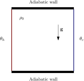
Figure 3: Differentially heated cavity test. Computational domain and boundary conditions.

Rayleigh	$\mathbf{g}$	$\rho_{0}$	$\alpha$	$\beta$	$\nu$
$10^{3}$	$\left(0,-9.81\right)^{T}$	$1$	$6.836\cdot 10^{-3}$	$3.4112\cdot 10^{-3}$	$4.874\cdot 10^{-3}$
$10^{4}$			$2.171\cdot 10^{-3}$		$1.541\cdot 10^{-3}$
$10^{5}$			$6.836\cdot 10^{-4}$		$4.874\cdot 10^{-4}$
$10^{6}$			$2.171\cdot 10^{-4}$		$1.541\cdot 10^{-4}$
$10^{7}$			$6.836\cdot 10^{-5}$		$4.874\cdot 10^{-5}$

Table 2: Differentially heated cavity test. Operating conditions.

The staggered mesh employed has $5172$ primal elements. The simulations were run considering the numerical parameters $p=2$, $p_{\gamma}=0$, i.e. we use piecewise quadratic polynomials in space and a first order scheme in time. The steady state stopping criterion is defined as

$$\frac{1}{\Delta t}\left\|\mathbf{v}^{n+1}-\mathbf{v}^{n}\right\|_{L^{2}\left(\Omega\right)}\leq 10^{-4}.$$ (103)

In order to analyze and compare the numerical results with available data in the literature, let us introduce the Nusselt number at the heated walls:

$$Nu_{\Gamma}=\frac{1}{\left|\Gamma\right|}\int_{{\Gamma}}Nu_{\mathrm{loc}}\,dA,\quad Nu_{\mathrm{loc}}=\frac{\kappa\,L}{\kappa_{0}\left(\theta_{h}-\theta_{c}\right)}\frac{\partial\theta}{\partial\vec{n}},$$ (104)

where $\Gamma$ refers to one of the heated walls, $L$ denotes the characteristic length and $\kappa$ is the thermal conductivity with $\kappa_{0}=\kappa\left(\theta_{0}\right)$.

The Nusselt numbers obtained at both heated walls using the fully Eulerian and the Eulerian-Lagrangian schemes are shown in Table 3. The average values presented in [96], [97], [98], [99] and [6] have been included for comparison purposes. To avoid overestimation of the Nusselt number by the Eulerian-Lagrangian scheme we need to bound the time step. More precisely, the time step given by (97) is halved, thus allowing the small structures embedded in the flow to be properly tracked.

Ra	STIN2D Eu.		STIN2D EL		Ref. [96]	Ref. [97]	Ref. [98]	Ref. [99]	Ref. [6]
	$\Gamma_{h}$	$\Gamma_{c}$	$\Gamma_{h}$	$\Gamma_{c}$	Average	Average	Average	Average	Average
$10^{3}$	$1.1199$	$1.1199$	$1.1212$	$1.1212$	$1.118$	$1.117$	$1.1149$	$1.117$	$1.112$
$10^{4}$	$2.2471$	$2.2471$	$2.2486$	$2.2486$	$2.243$	$2.243$	$2.2593$	$2.254$	$2.198$
$10^{5}$	$4.5283$	$4.5302$	$4.6605$	$4.5302$	$4.519$	$4.521$	$4.4832$	$4.598$	$4.465$
$10^{6}$	$8.8651$	$8.8655$	$8.8592$	$8.8595$	$8.800$	$8.806$	$8.8811$	$8.976$	$8.783$
$10^{7}$	$16.8394$	$16.8428$	$16.7684$	$16.7714$	$--$	$16.40$	$16.3869$	$16.656$	$16.46$

Table 3: Differentially heated cavity (DHC) test. Comparison of the Nusselt number obtained with the Eulerian (Eu) and Eulerian-Lagrangian (EL) advection scheme with available reference solutions from the literature.

Ra	STIN2D Eu.	STIN2D EL	Ref. [96]	Ref. [97]	Ref. [98]	Ref. [99]
$10^{3}$	$3.7227$	$3.7324$	$3.679$	$3.692$	$3.6962$	$3.686$
$10^{4}$	$19.6342$	$19.6372$	$19.51$	$19.63$	$19.6177$	$19.79$
$10^{5}$	$68.9334$	$68.9526$	$68.22$	$68.85$	$68.6920$	$70.63$
$10^{6}$	$220.603$	$220.212$	$216.75$	$221.6$	$220.8331$	$227.11$
$10^{7}$	$701.051$	$700.679$	$--$	$702.3$	$703.2526$	$714.48$

Table 4: Differentially heated cavity (DHC) test. Comparison of the normalized maximum vertical velocity at $y=0.5$ obtained with the Eulerian (Eu) and Eulerian-Lagrangian (EL) advection schemes with available reference solutions from the literature.

Ra	STIN2D Eu.	STIN2D EL	Ref. [96]	Ref. [98]	Ref. [99]
$10^{3}$	$3.6736$	$3.6828$	$3.634$	$3.6493$	$3.489$
$10^{4}$	$16.1856$	$16.1877$	$16.2$	$16.1798$	$16.12$
$10^{5}$	$34.8869$	$34.896$	$34.81$	$34.7741$	$33.39$
$10^{6}$	$64.8511$	$64.9075$	$65.33$	$64.6912$	$65.40$
$10^{7}$	$148.681$	$149.561$	$--$	$145.2666$	$143.56$

Table 5: Differentially heated cavity (DHC) test. Comparison of the normalized maximum horizontal velocity at $x=0.5$ obtained with the Eulerian (Eu) and Eulerian-Lagrangian (EL) advection schemes with available reference solutions from the literature.

Figures 4-8 depict the numerical solution of temperature and velocity. Moreover, streamlines and vorticity contours are shown in Figure 9. A good agreement is observed between the results computed with our two different advection schemes (Eulerian upwind scheme and Eulerian-Lagrangian scheme) and with the data reported in literature (see [100, 97, 101, 102, 98, 99, 103, 6]). Comparison with available data is also carried out considering the vertical and horizontal velocities in the mid planes, which have been plotted in Figures 11-10. Furthermore, the normalized maximum velocities in the mid plane are reported in Tables 4-5.

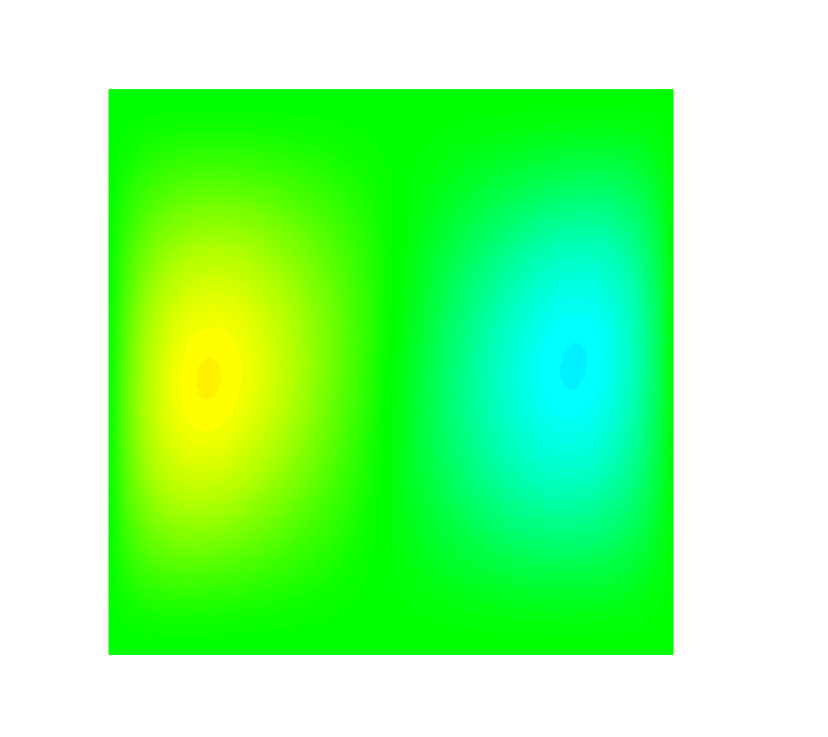
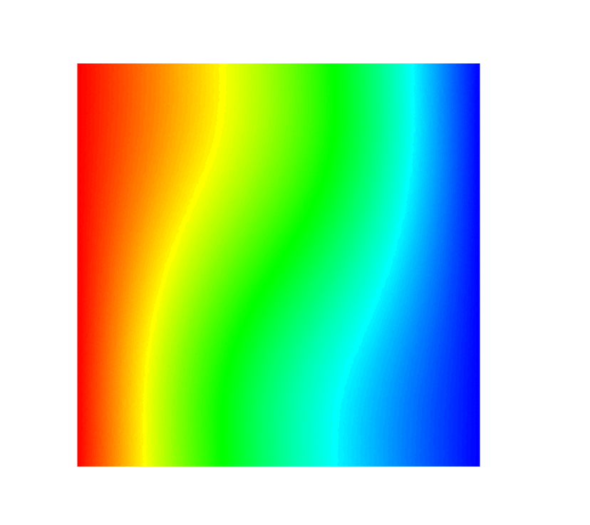
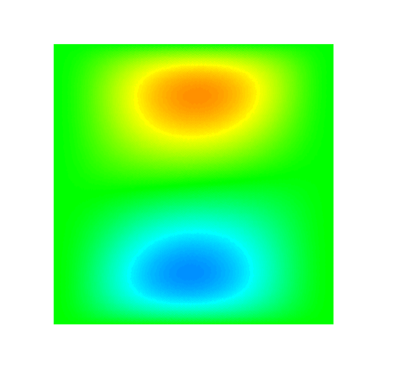
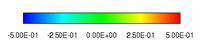
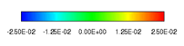
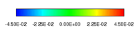
Figure 4: DHC. From left to right: temperature, horizontal and vertical velocity contours at $Ra=10^{3}$. Top: Eulerian advection scheme. Bottom: Eulerian-Lagrangian advection scheme.

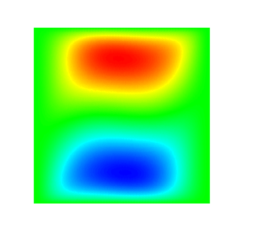
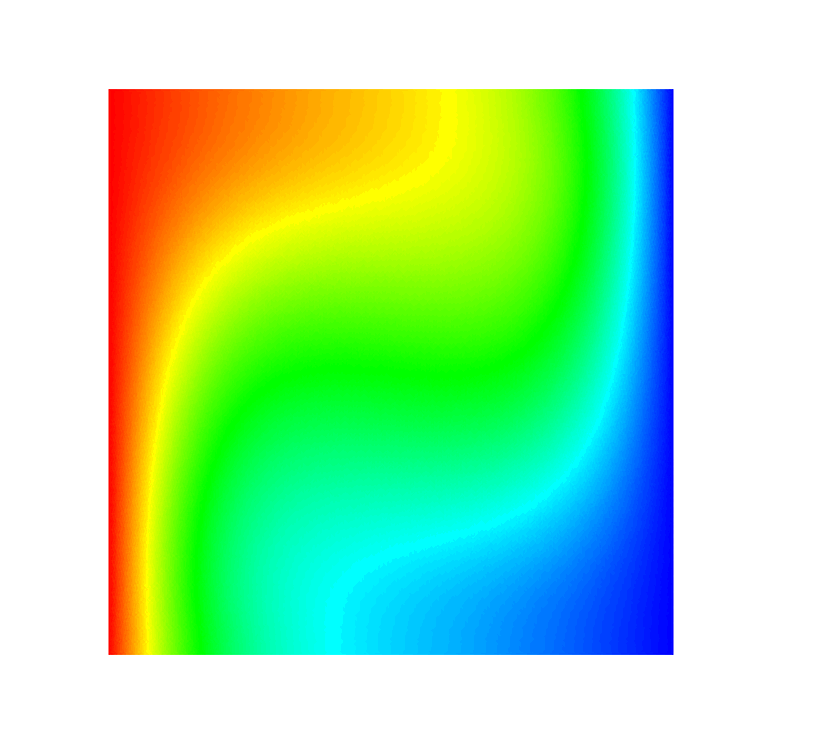
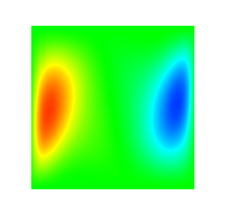
Figure 5: DHC. From left to right: temperature, horizontal and vertical velocity contours at $Ra=10^{4}$. Top: Eulerian advection scheme. Bottom: Eulerian-Lagrangian advection scheme.

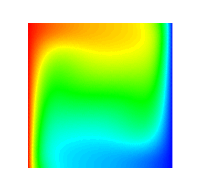
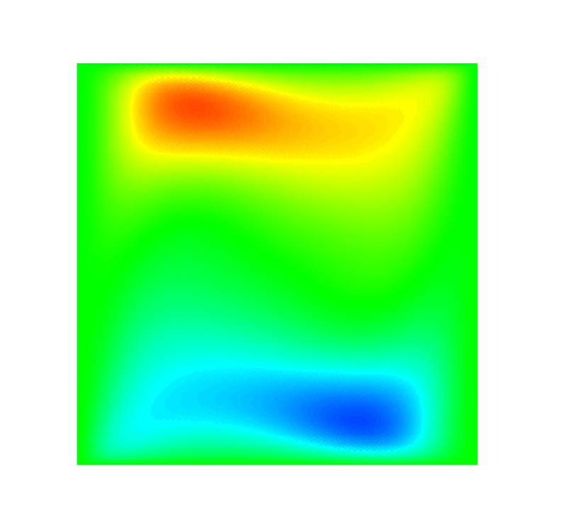
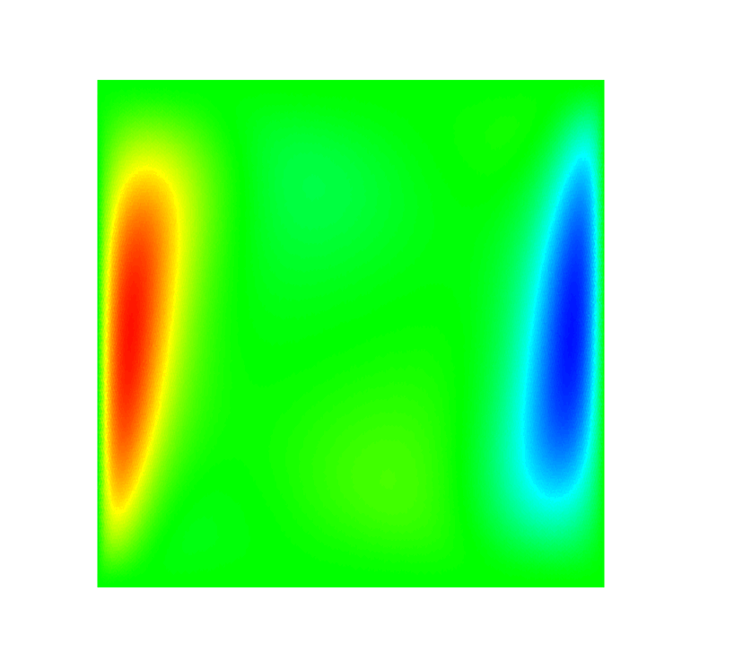
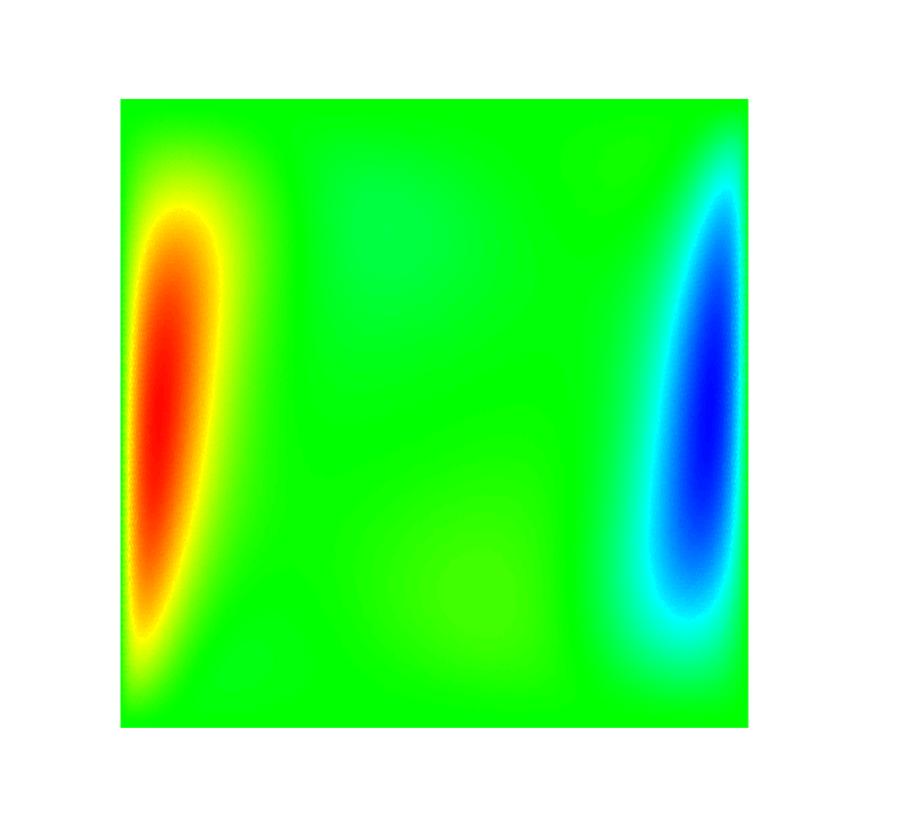
Figure 6: DHC. From left to right: temperature, horizontal and vertical velocity contours, $Ra=10^{5}$. Top: Eulerian advection scheme. Bottom: Eulerian-Lagrangian advection scheme.

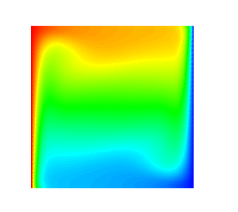
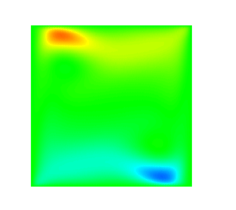
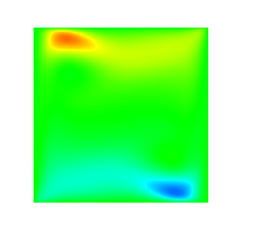
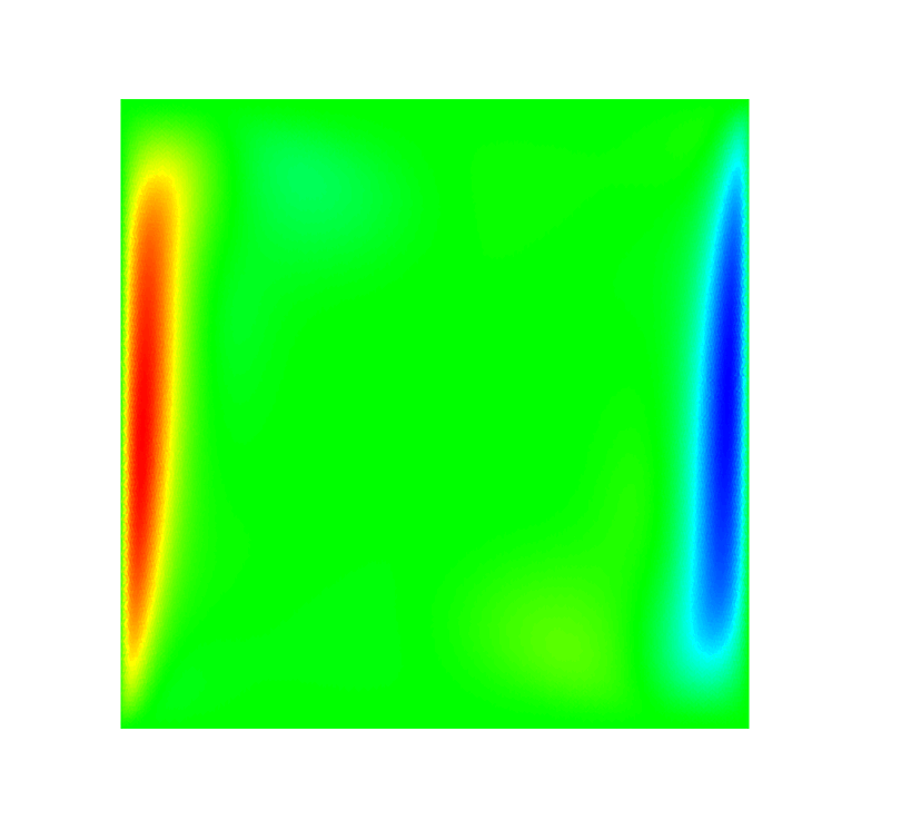
Figure 7: DHC. From left to right: temperature, horizontal and vertical velocity contours, $Ra=10^{6}$. Top: Eulerian advection scheme. Bottom: Eulerian-Lagrangian advection scheme.

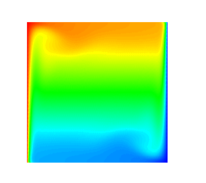
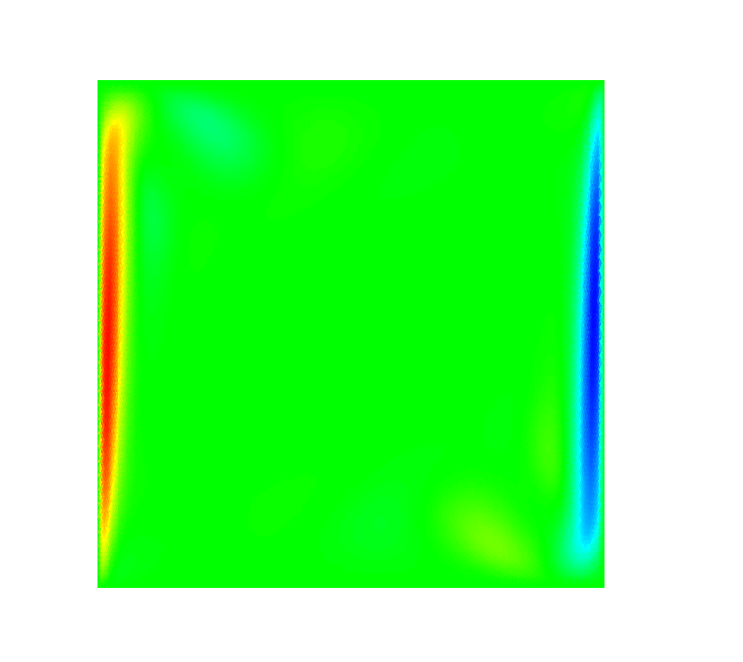
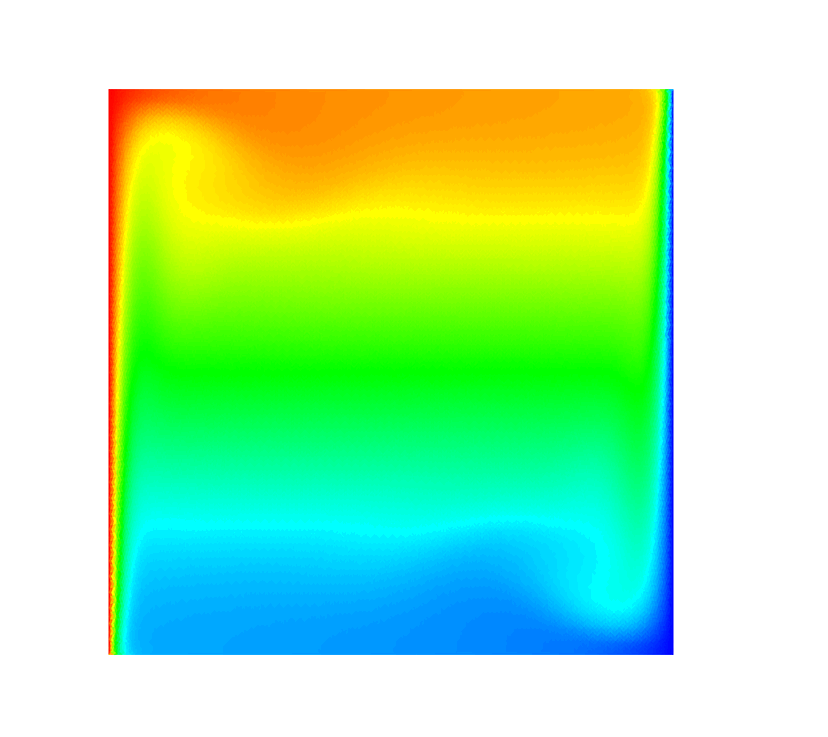
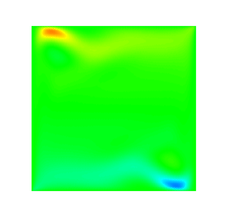
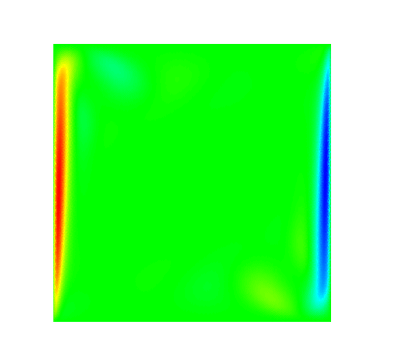
Figure 8: DHC. From left to right: temperature, horizontal and vertical velocity contours, $Ra=10^{7}$. Top: Eulerian advection scheme. Bottom: Eulerian-Lagrangian advection scheme.

$Ra=10^{3}$                               $Ra=10^{4}$

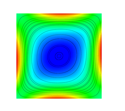
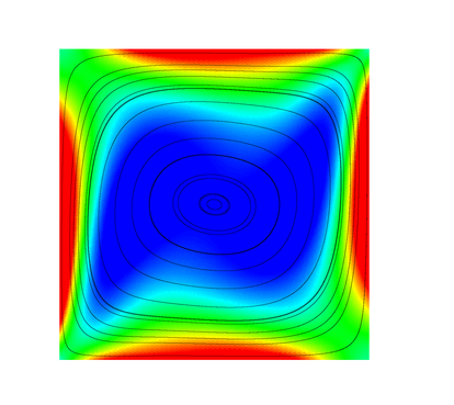
$Ra=10^{5}$                               $Ra=10^{6}$                               $Ra=10^{7}$

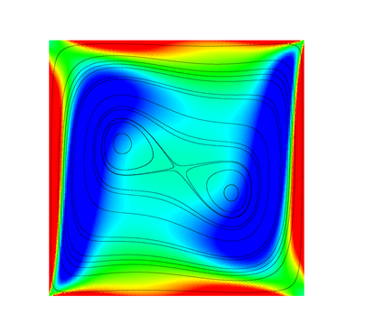
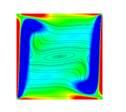
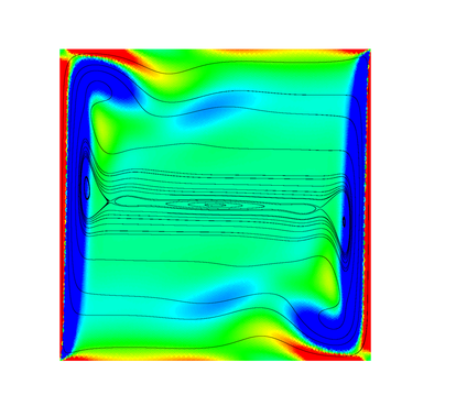
Figure 9: DHC. Streamlines and vorticity contours obtained using the Eulerian-Lagrangian approach for advection.

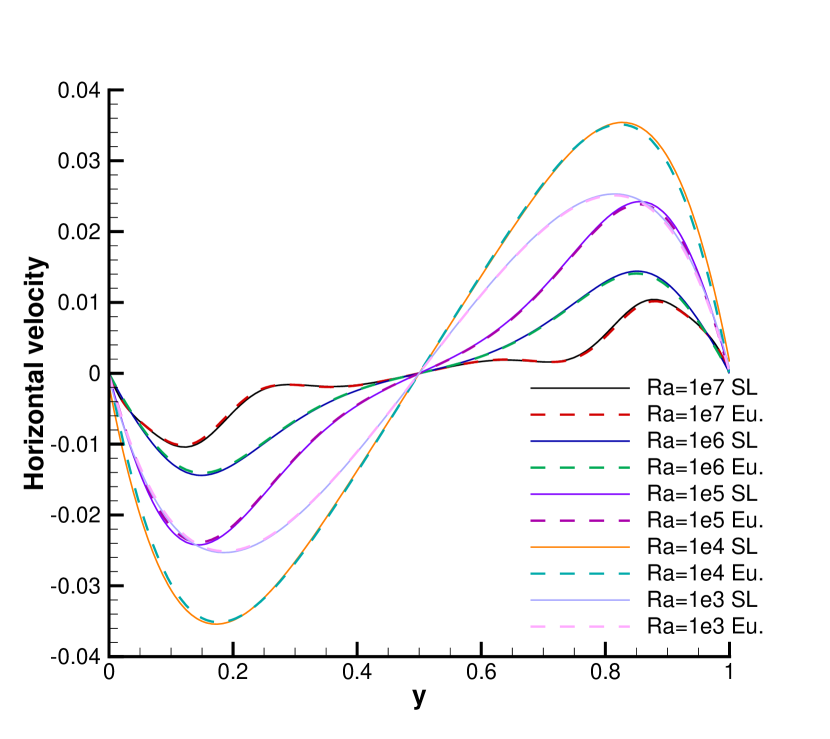
Figure 10: DHC. Horizontal velocity, $x=0.5$.

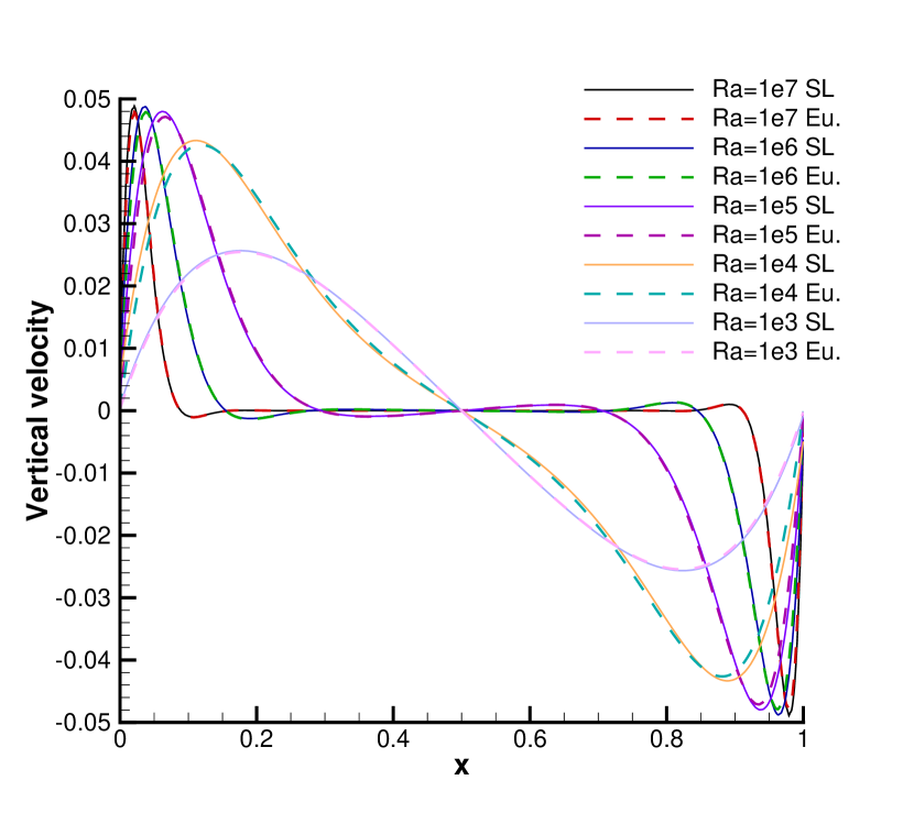
Figure 11: DHC. Vertical velocity, $y=0.5$.

6.3 Cavity with differentially heated cylinders

We propose a modification to the previous test case on a more complex geometry where six cylinders of radius $r=0.1$ are subtracted from the square cavity, see Figure 12.

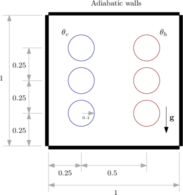
Figure 12: Cavity with differentially heated cylinders. Computational domain and boundary conditions.

We assume an initial fluid at rest with constant temperature $\theta_{0}=293.15K$, density $\rho_{0}=1$ and $\mathbf{g}=\left(0,-9.81\right)^{T}$. Dirichlet boundary conditions are imposed on the cylinder walls, where the exact temperature is prescribed. Specifically, the left cylinders are cooled with $\theta_{c}=292.65K$, whereas the right ones are heated with $\theta_{h}=293.65K$. The remaining walls are assumed to be adiabatic. The computational domain is paved with a primal mesh of $18396$ elements and two different settings are considered, according to the diffusion coefficients: $\left(\mu_{T_{1}},\alpha_{T_{1}}\right)=\left(4.874\cdot 10^{-4},6.86\cdot 10^{-4}\right)$ and $\left(\mu_{T_{2}},\alpha_{T_{2}}\right)=\left(4.874\cdot 10^{-6},6.865\cdot 10^{-6}\right)$.

Figure 13 shows the contour plots of temperature, horizontal and vertical velocity obtained for the first setup using the fully Eulerian and the Eulerian-Lagrangian schemes with $p=2$, $\Theta=0.51$. A good agreement is observed between the two approaches. To illustrate the mesh convergence, the results corresponding to a mesh refinement factor of 2 are included as well.

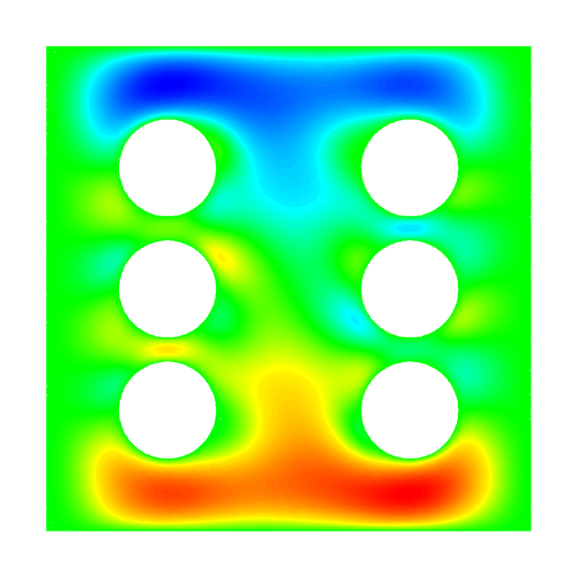
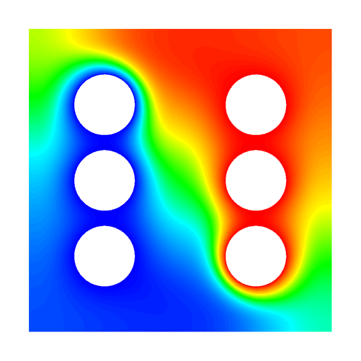
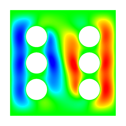
Figure 13: Cavity with differentially heated cylinders. From left to right: temperature, horizontal and vertical velocity contours for $\left(\mu,\alpha\right)=\left(4.874\cdot 10^{-4},6.86\cdot 10^{-4}\right)$. Top: Eulerian advection scheme. Center: Eulerian-Lagrangian advection scheme. Bottom: Eulerian advection scheme with mesh refinement factor 2.

The reduced viscosity coefficient defined in the second setup leads to an unsteady flow field, developing many secondary vortices and flow instabilities. The simulation was run relying on the Eulerian-Lagrangian scheme which reduces the computational cost. Nevertheless, to capture the sub-scale structures of the flow, we have fixed the time step to be $5/2$ times greater than the one computed from (97). In Figure 14 we depict the results obtained at different output times.

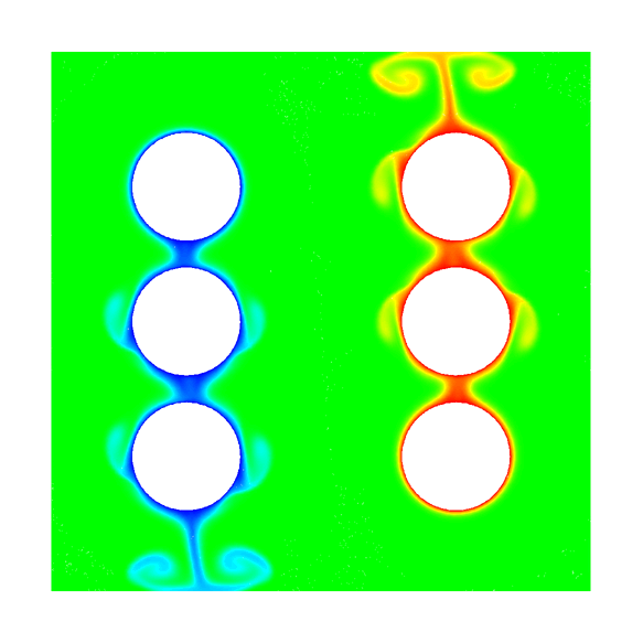
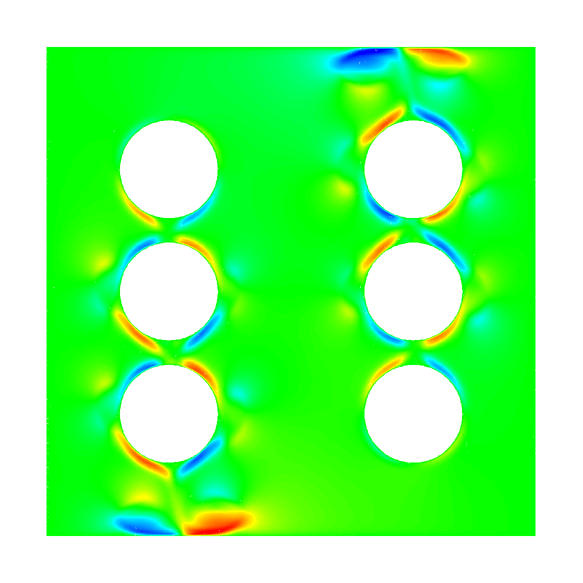
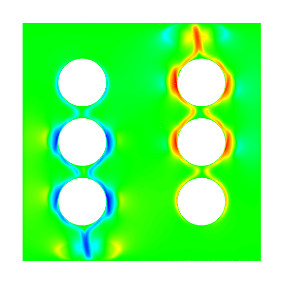
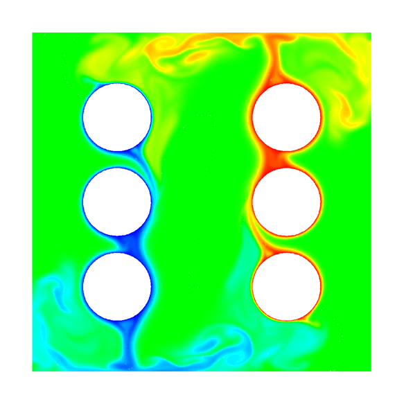
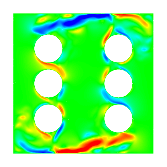
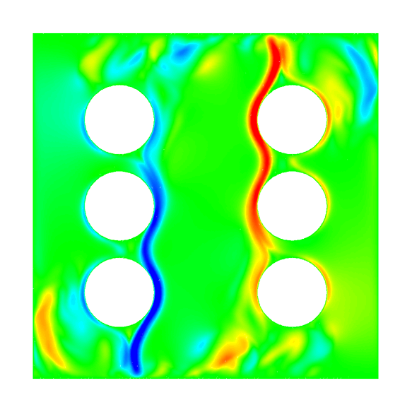
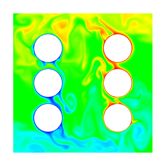
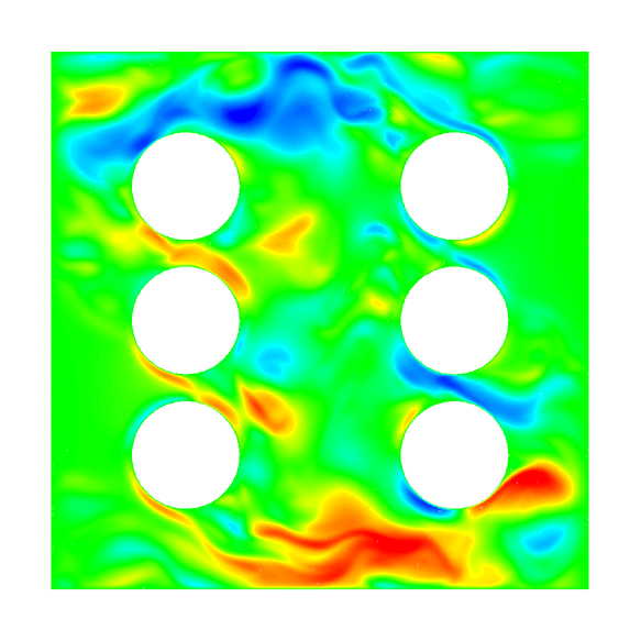
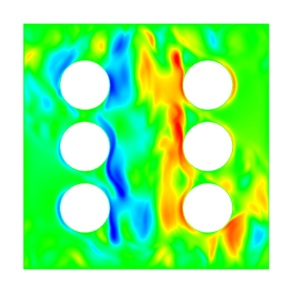
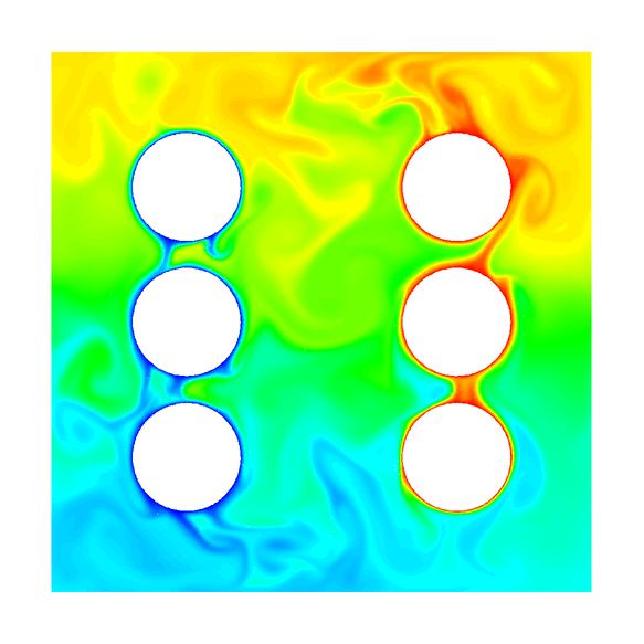
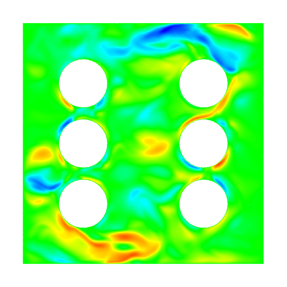
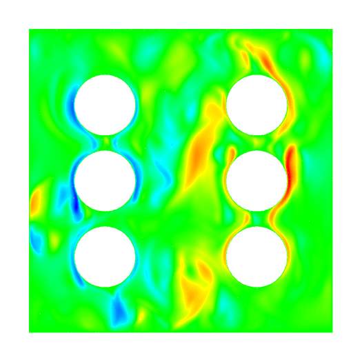
Figure 14: Cavity with differentially heated cylinders. From left to right: temperature, horizontal and vertical velocity contours for $\left(\mu,\alpha\right)=\left(4.874\cdot 10^{-4},6.86\cdot 10^{-4}\right)$. From top to bottom: output time $20s$, $50s$, $80s$, $200s$.

6.4 Warm bubble in two space dimensions

As fourth test case we propose to solve the smooth rising bubble benchmark problem introduced in [5], which has been widely used to test numerical solvers of thermal convection problems (see [104, 105, 106, 10]). This problem assumes an initial fluid at rest and a warm bubble embedded in it. During the simulation, the bubble will rise and deform gradually acquiring a mushroom-type shape and later also developing secondary Kelvin-Helmholtz-type flow instabilities. Although no exact solution is known, the analysis of the results can be qualitatively performed taking into account the symmetry of the bubble as well as other numerical results available in the literature.

The computational domain is a square of $1$km side length. The bubble is initially placed at $\mathbf{x}_{b}=(0.5,0.35)$ km and is assigned the following initial temperature fluctuation:

$$\theta(\mathbf{x},0)-\theta_{0}=\left\{\begin{array}[]{lr}0,&\mathrm{if}\;r>r_{b},\\ \dfrac{\theta_{b}}{2}\left[1+\cos\left(\dfrac{\pi r}{r_{b}}\right)\right],&\mathrm{if}\;r\leq r_{b},\end{array}\right.$$ (107)

with $r=\left\|\mathbf{x}-\mathbf{x}_{b}\right\|$ representing the distance from the center of the bubble, $r_{b}=0.25$km being its radius and $\theta_{b}=0.5$K denoting the maximal initial amplitude of the perturbation. The temperature perturbation (107) is imposed over a background temperature which is assumed to be $\theta_{0}=303.15$K.

The use of the Eulerian scheme, without any limiter, to solve Euler equations may produce high velocity gradients in the boundary of the warm bubble. To avoid the growth of instabilities in the numerical solution, we may add a small artificial viscosity. However, as already discussed in [104, 105, 107], this leads to a smoothness of the boundary of the bubble, that is affected by numerical dissipation. Figure 15 shows the results obtained at time instants $t\in\left\{600,700,800,900\right\}$s using a constant artificial viscosity with $\mu=10^{-6}$ and a very coarse primal mesh composed of only $5172$ triangles. We run the test problem using piecewise polynomials of degree $p=4$ in order to represent the discrete solution. We observe that the evolution of the main shape of the bubble agrees with the results available in literature. Moreover, for large times, long-wave oscillations arise on top of the main structure.

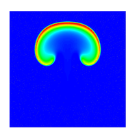
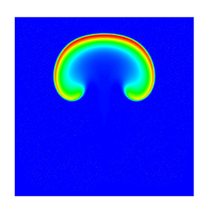
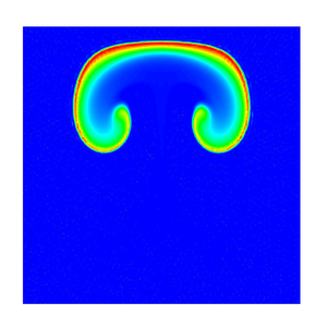
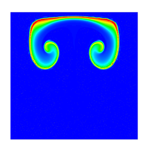
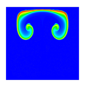
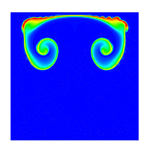
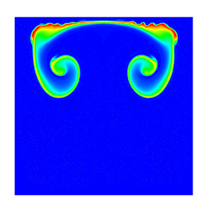
Figure 15: Warm bubble test in 2D: temperature contours. $\mu=10^{-6}$, $p=4$, $\Theta=0.51$. Left: Eulerian advection scheme. Right: Eulerian-Lagrangian advection scheme. From top to bottom: output time $600$s, $700$s, $800$s, $900$s.

An alternative strategy to get a stable solution with very little numerical dissipation is the use of a Eulerian-Lagrangian advection scheme. In this case we do not need to add any artificial viscosity, even for high order DG discretization. Moreover, the use of this methodology yields to a reduction on the computational cost of the algorithm. For the test case shown in this section, the implementation based on the Eulerian-Lagrangian advection scheme was overall 4.3 times faster than the implementation based on the classical Eulerian advection scheme. This improvement is related to the increase of the time step size allowed by the Eulerian-Lagrangian approach.

The results obtained using the Eulerian-Lagrangian approach for $\mu=0$ are depicted in Figure 16 for the intermediate time instants $t\in\left\{600,700,800,900\right\}$s. We observe that the solution at the beginning of the simulation is almost symmetric, where the small discrepancies which arise are due to the unstructured and non-symmetric mesh that is used. After $800$s mushroom-shaped structures start to grow from the cap of the main shape. Moreover, for long times small vortex structures develop on the top of the long waves resulting in secondary Kelvin-Helmholtz instabilities. At this step the flow becomes completely turbulent and therefore the initial symmetry is lost. The comparison against the results depicted in Figure 15, where a non-zero artificial viscosity was employed, show that the viscosity required by the Eulerian scheme to provide a stable solution is already too high to properly capture the small vortexes generated within the fluid flow. Therefore, the use of a Eulerian-Lagrangian scheme with zero viscosity is a key point in order to avoid the damping of Kelvin-Helmholtz instabilities. Furthermore, Figure 16, which shows the results obtained considering spatial polynomial degrees $2$ and $4$, highlights the importance of employing a high order scheme in order to capture the small secondary vortex structures.

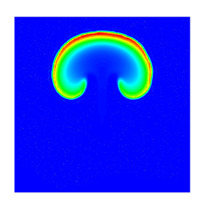
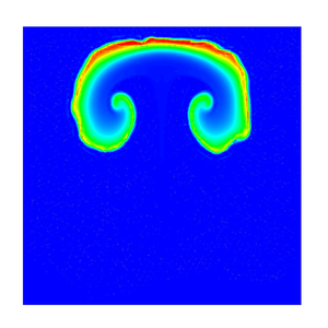
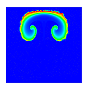
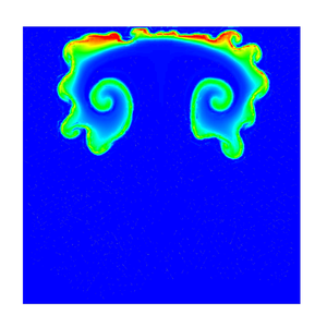
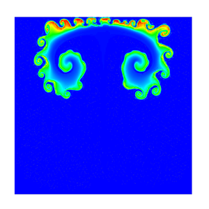
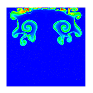
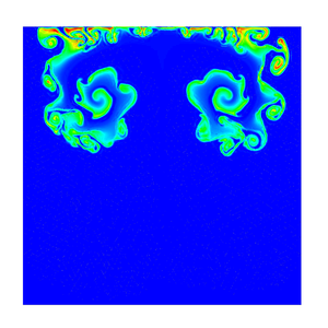
Figure 16: Warm bubble test in 2D: temperature contours. Eulerian-Lagrangian advection scheme, $\mu=0$. Left: $p=2$, $\Theta=0.51$. Right: $p=4$, $\Theta=0.51$. From top to bottom: output time $600$s, $700$s, $800$s, $900$s.

6.5 Warm bubble in three space dimensions

We now extend the warm bubble test to a three-dimensional domain, following the setup described in [107, 106]. To this end, we define the computational domain $\Omega=\left[0,1\right]\times\left[0,1\right]\times\left[0,1.5\right]$ km. The warm bubble is initially located at $\mathbf{x}_{b}=(0.5,0.5,0.35)$ and the temperature is defined by (107) with $r=\left\|\mathbf{x}-\mathbf{x}_{b}\right\|$. Furthermore, we consider $r_{b}=0.25$km, $\theta_{0}=303.15$K and zero viscosity, i.e. $\nu=0$.

The computational mesh counts a total number of $1,331,442$ primal tetrahedral elements and we use piecewise polynomials of degree $p=3$ for the representation of the discrete solution. This amounts to a total of $26,628,840$ degrees of freedom for the pressure. The computer code was parallelized using the MPI standard and the simulation was run on 960 CPU cores of the SuperMUC-NG supercomputer at the LRZ in Garching, Germany. Figures 17-18 depict the numerical results obtained at different time instants. The three-dimensional results mimic the behavior of the warm bubble already observed in the two-dimensional setting. The differences in temperature induce a velocity field in the flow that will produce an upward movement of the bubble, which yields the development of the main mushroom-shaped structure for the temperature. However, we observe that the Kelvin-Helmholtz instabilities arising in the bi-dimensional test case do not appear in 3D. This may be due to the coarse grid resolution used here. As already noticed in Figure 16, an increase in the spatial order of accuracy of the scheme could improve the final results.

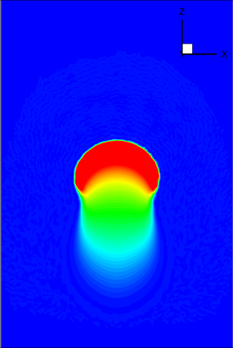
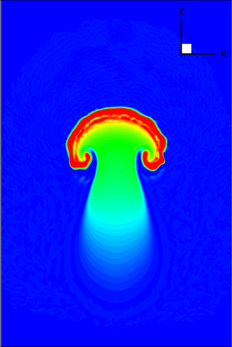
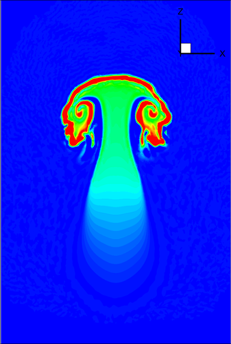
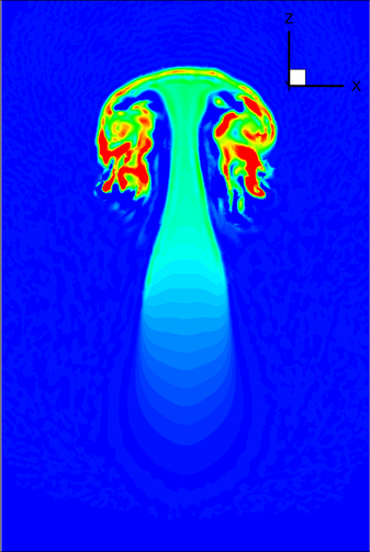
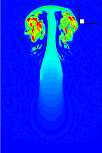
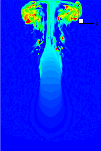
Figure 17: Warm bubble test in 3D: temperature contours in the plane $x=0.5$ at times $t\in\left\{400,500,600,700,800,900\right\}$s.

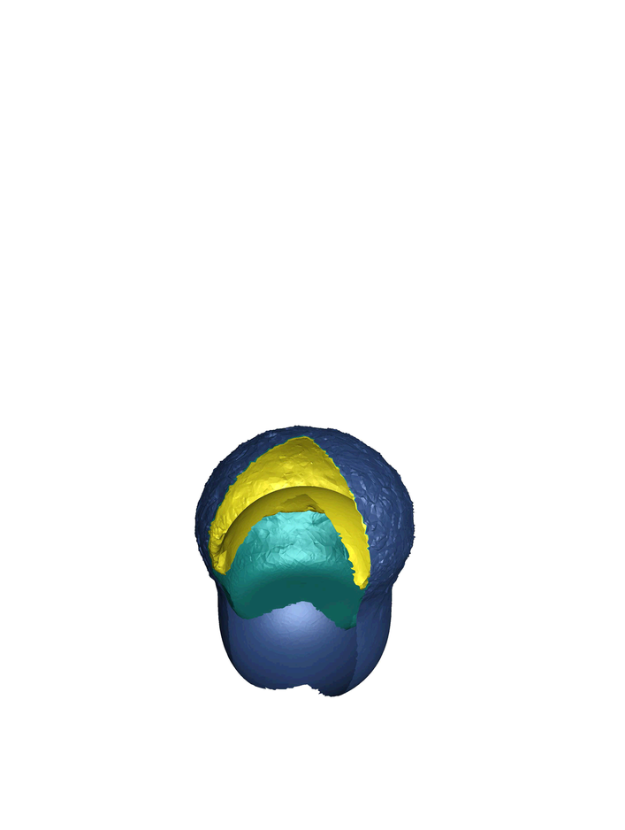
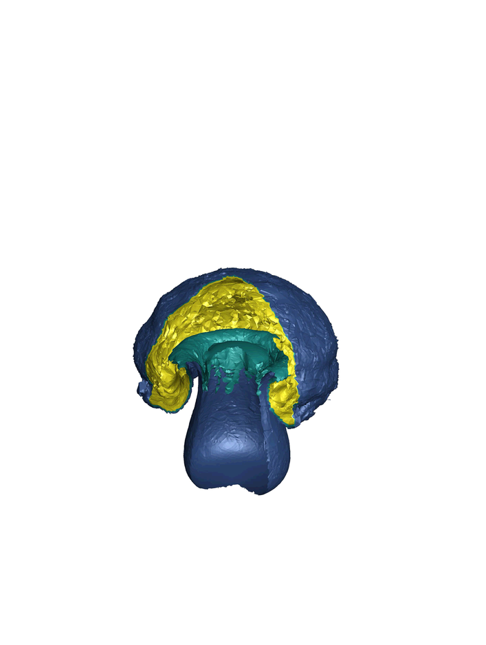
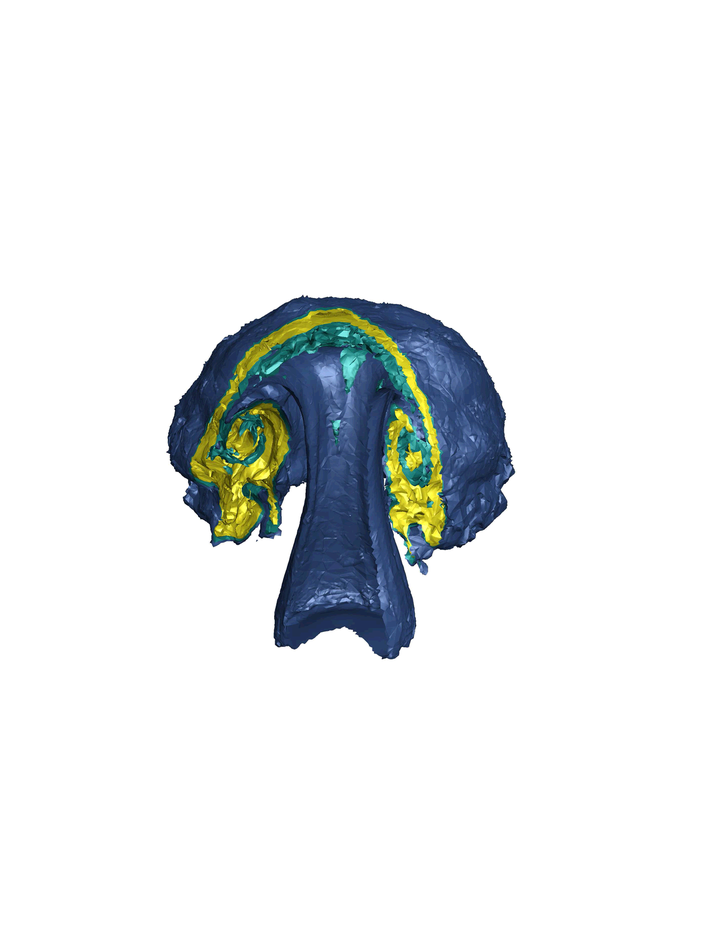
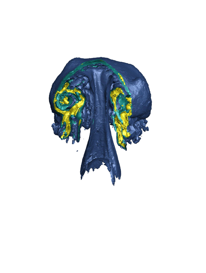
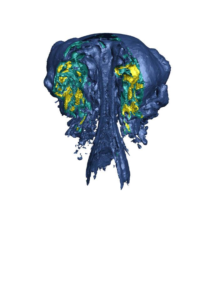
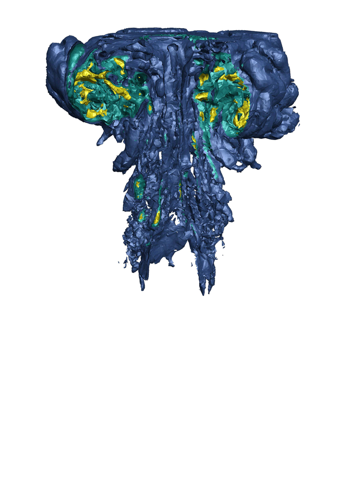
Figure 18: Warm bubble test in 3D: isosurfaces of $\theta$ at times $t\in\left\{400,500,600,700,800,900\right\}$s.

6.6 Comparison of incompressible and compressible flow solvers for a Gaussian bubble in 2D

In this section we compare the results obtained with both the incompressible and the compressible flow solver by considering a rising bubble test defined in the computational domain $\Omega=\left[-0.5,1.5\right]\times\left[-0.5,1.5\right]$ with periodic boundary conditions on the lateral boundaries. The initial temperature profile is the one of a Gaussian bubble and reads

$$\theta(\mathbf{x},0)=\left\{\begin{array}[]{lr}386.48=\theta_{0},&\mathrm{if}\;r>r_{b},\\ \dfrac{p_{0}}{R\left(1.0-0.1e^{-\frac{r^{2}}{\sigma^{2}}}\right)},&\mathrm{if}\;r\leq r_{b},\end{array}\right.$$ (110)

where $r=\left\|\mathbf{x}-\mathbf{x}_{b}\right\|$ is the distance from the center of the bubble $\mathbf{x}_{b}=(0.5,0.35)$; $r_{b}=0.25$ is the bubble radius and $\sigma=2$ is a halfwidth; $p_{0}=10^{5}$ is the initial pressure; and $R=287$ denotes the specific gas constant. Moreover, we consider the following operating conditions:

$$c_{\pi}=1004.5,\quad\gamma=1.4,\quad\mu=1.68\cdot 10^{-5},\quad\alpha=2.625\cdot 10^{-5},\quad\beta=2.587\cdot 10^{-3},\quad\mathbf{g}=\left(0,-9.81\right)^{T}.$$

Consequently, the main dimensionless numbers are given by

$$Re=8.049\cdot 10^{2},\quad Pr=0.71,\quad Gr=7.603\cdot 10^{6},\quad Pe=5.715\cdot 10^{2},\quad Ra=5.399\cdot 10^{5},\quad\beta\Delta\theta=1.72\cdot 10^{-3},\quad M\sim 10^{-2}.$$

The simulations were run in the Eulerian framework taking $p=3$, $\Theta=0.51$. The primal mesh consists of $3602$ control volumes. Figures 19, 20 and 21 depict the numerical results at output times $t\in\left\{10,20,30\right\}$. As expected, we notice that the temperature and velocity contours obtained with the incompressible (INS) and compressible (CNS) flow solver are really close to each other. This is confirmed by a more detailed analysis of the numerical solution computed along specific cuts along the $x-$axis in the computational domain, as we can observe in the plots included at the right hand side of Figures 19-21. Therefore, for a flow regime verifying the hypothesis related to the Boussinesq approximation, we can use both sets of equations to solve natural convection problems obtaining similar results. One of the main advantages of the incompressible model is the lower computational cost compared to the compressible one, that is approximately seven times slower. Moreover, the algorithm for the incompressible model is much simpler, since we can neglect density variations, hence avoiding the non-linearity of the system presented for the compressible case (see Section 4.2). On the other hand, the compressible model is more general. Since the algorithm has been developed to perform well at all Mach numbers, see [4], we are able to simulate a broader variety of problems including both small and large temperature fluctuations.

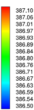
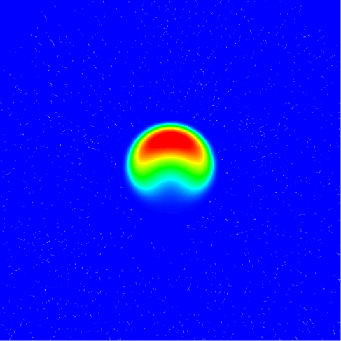
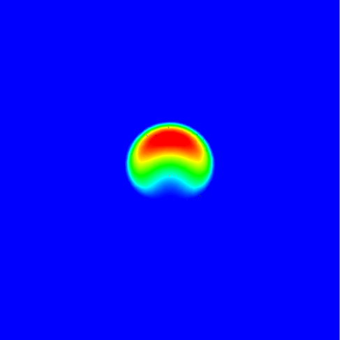
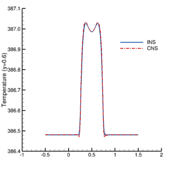
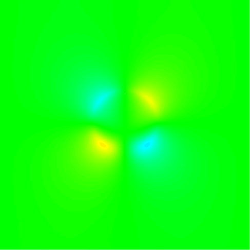
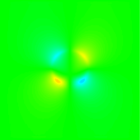
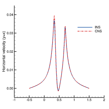
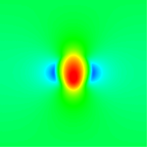
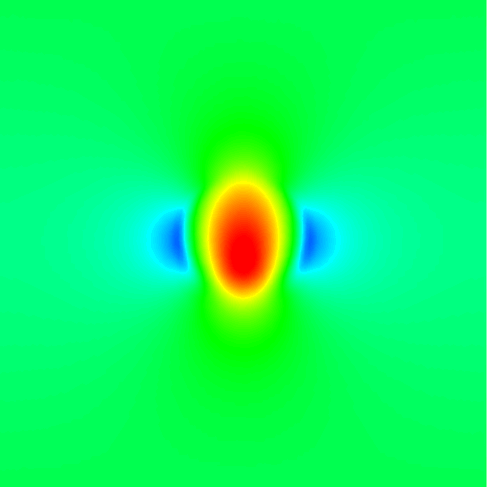
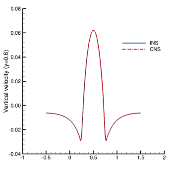
Figure 19: Gaussian bubble test. From top to bottom: temperature, horizontal and vertical velocity, $t=10s$. Left: incompressible flow solver. Center: compressible flow solver. Right: profile obtained over a specific line.

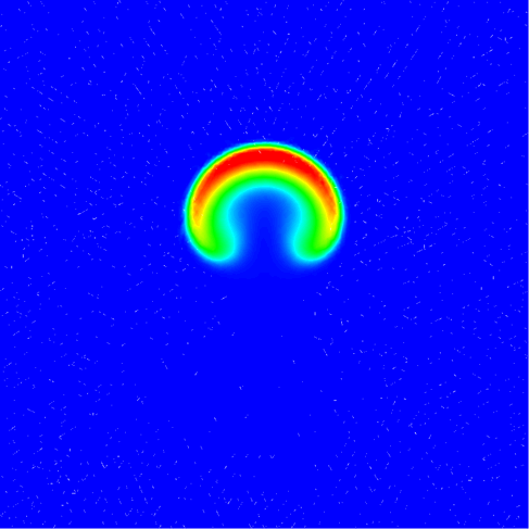
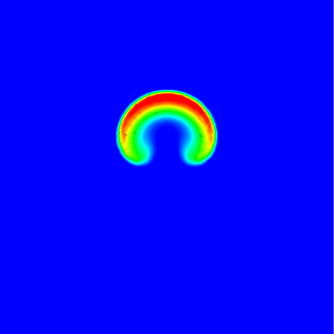
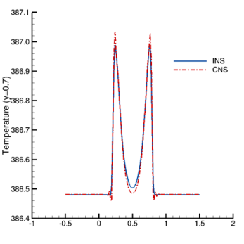
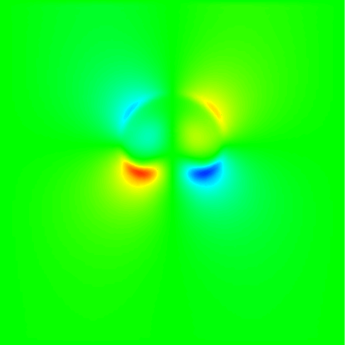
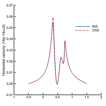
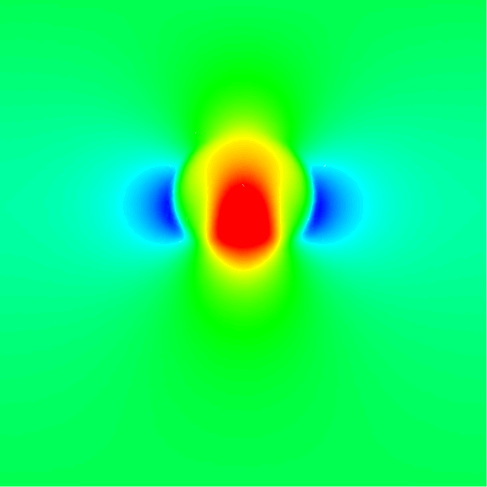
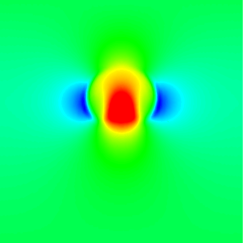
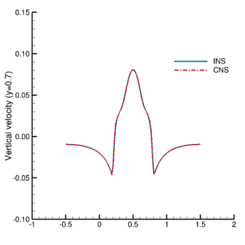
Figure 20: Gaussian bubble test. From top to bottom: temperature, horizontal and vertical velocity, $t=15s$. Left: incompressible flow solver. Center: compressible flow solver. Right: profile obtained over a specific line.

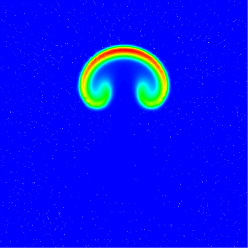
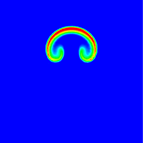
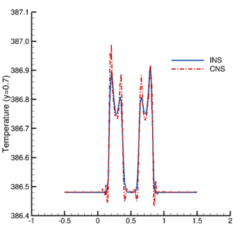
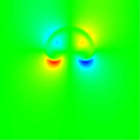
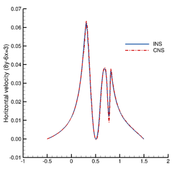
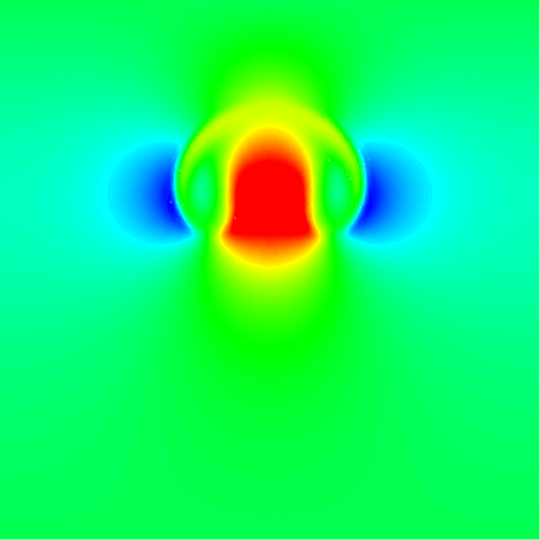
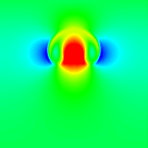
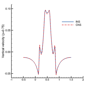
Figure 21: Gaussian bubble test. From top to bottom: temperature, horizontal and vertical velocity, $t=20s$. Left: incompressible flow solver. Center: compressible flow solver. Right: profile obtained over a specific line.

As second part of this test case, we compare the results obtained considering two different time discretizations. Figure 22 reports the numerical solution computed with the incompressible model, when using two sets of space-time basis functions, namely $(p,p_{\gamma})=(3,1)$ and $(p,p_{\gamma})=(3,2)$. We can observe that the theta method produces the same results of the second and third order accurate space-time DG schemes.

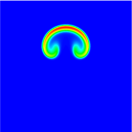
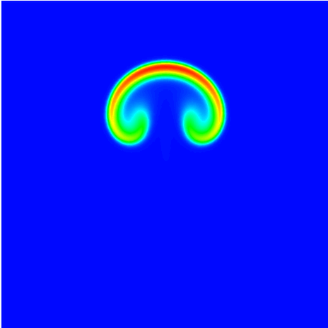
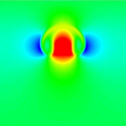
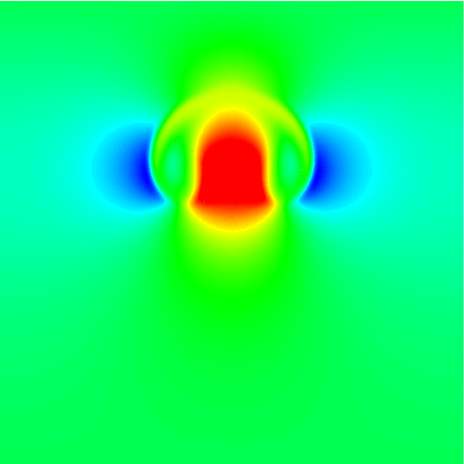
Figure 22: Gaussian bubble test. From top to bottom: temperature, horizontal and vertical velocity, $t=20s$. Left: $p=3$, $\Theta=0.51$. Center: $(p,p_{\gamma})=(3,1)$. Right: $(p,p_{\gamma})=(3,2)$.

6.7 Locally heated cavity

As last test case, we introduce a locally heated cavity test which looks similar to the classical one reported in Section 6.2. Positive and negative heat sources on the bottom and upper wall, respectively, are imposed as boundary conditions. Due to the physical instability of the chosen boundary conditions, we drive the generation of the rising/falling structures by setting sinusoidal functions. The computational domain $\Omega=[-0.8,0.8]\times[-0.45,0.45]$, is initially discretized using $5172$ triangular elements. Then, we perform some refinements in order to show mesh convergence. We use adiabatic no-slip walls for the left and right boundaries and we prescribe

$$\mathbf{v}=\bm{0},\quad\theta(x,y,t)=\left\{\begin{array}[]{lr}0.1-0.1|\cos(16x)|,&\mathrm{if}\;y=-0.45,\\ -0.1+0.1|\sin(16x)|,&\mathrm{if}\;y=-0.45,\end{array}\right.$$ (111)

on the top and bottom boundaries. Finally, we set $\mathbf{g}=\left(0,-9.81\right)^{T}$, $\mu=10^{-4}$, $\alpha=10^{-3}$, and $p=3$. The resulting time evolution of the temperature for mesh refinements by a factor of $2,3,4$ and $5$ in each space dimension is reported in Figures 23-24. We can observe the generation of some mushroom-shape structures that arise from the flow that is only driven by the temperature boundary conditions. Later in time, they start to mix and to form complex substructures. Let us remark that, for refinement levels $2$ and $3$, we obtain essentially the same results up to $t=12s$. However, at $t=14s$ we encounter some small differences that become evident at the final time, see Figure 23. However, a good agreement is observed for long time solutions when increasing the mesh resolution, see Figure 24.

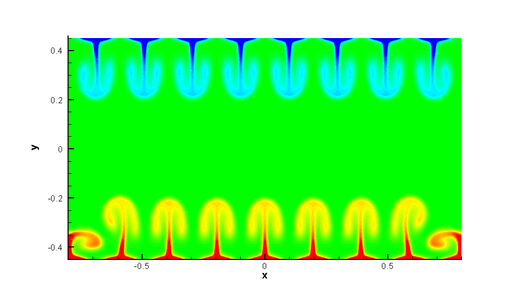
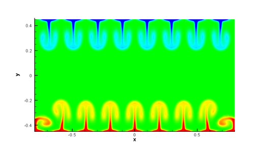
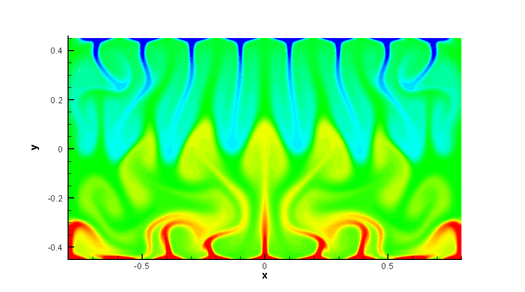
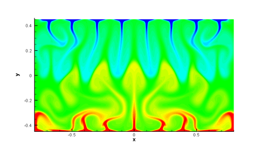
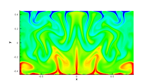
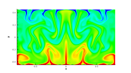
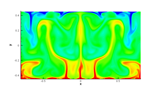
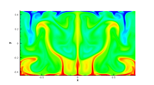
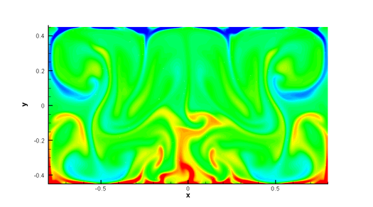
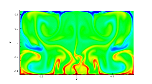
Figure 23: Locally heated cavity. From top to bottom: temperature profile at times $t\in\left\{5,10,12,14,17\right\}$. Left: mesh refinement factor 2. Right: mesh refinement factor 3.

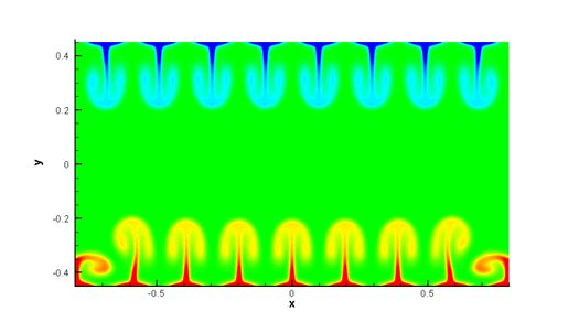
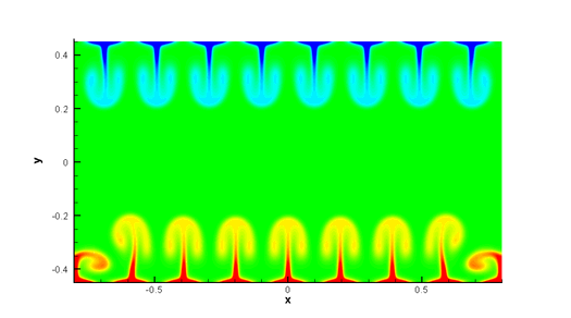
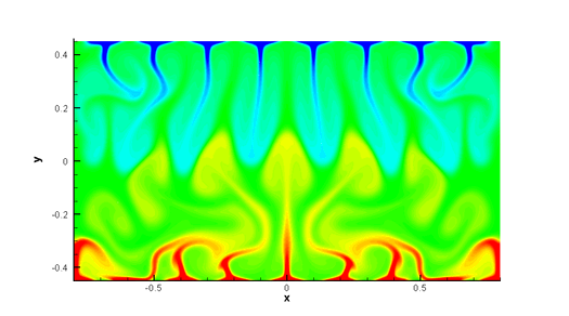
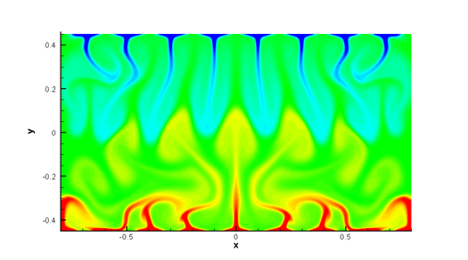
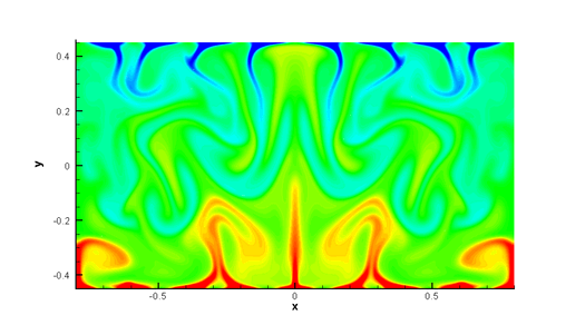
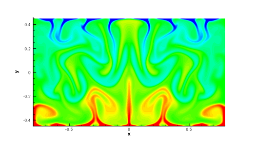
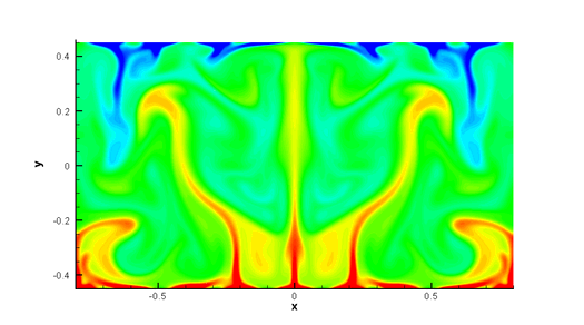
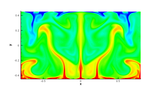
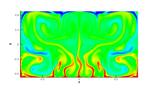
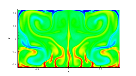
Figure 24: Locally heated cavity. From top to bottom: temperature profile at times $t\in\left\{5,10,12,14,17\right\}$. Left: mesh refinement factor 4. Right: mesh refinement factor 5.

7 Conclusions

In this work, we have presented a new high order accurate staggered semi-implicit discontinuous Galerkin finite element scheme for the solution of natural convection problems. The algorithm is based on the work proposed in [1, 3, 4]. A unified framework for the discretization of incompressible and compressible Navier-Stokes equations with gravity terms has been introduced. The computational cost of the global algorithm has been reduced thanks to the development of a novel Eulerian-Lagrangian approach for the treatment of the nonlinear convective terms, which leads to an unconditionally stable scheme for the incompressible Navier-Stokes system. Furthermore, the new methodology is able to handle flows with large temperature and velocity gradients. The final algorithms developed within this work have been assessed using several classical benchmarks, showing good agreement with the reference data. A detailed comparison between the fully Eulerian and the Eulerian-Lagrangian approaches for advection has been performed, highlighting the main advantages and drawbacks of both methodologies. Moreover, the numerical results obtained with the incompressible Navier-Stokes equations in combination with the Boussinesq approximation have also been validated against a numerical solution of the full compressible Navier-Stokes equations. We have shown computational results for a rising bubble in three space dimensions using more than 26 million spatial degrees of freedom, which clearly shows that the proposed computational approach can also be used on modern massively parallel distributed memory supercomputers. This test case has been set to demonstrate the potential capability of the proposed high order staggered semi-implicit DG algorithm for direct numerical simulations (DNS) on unstructured grids at moderate Reynolds numbers, i.e. the full resolution of all small scale structures present in the flow without the use of any turbulence models.

Future research will involve the development of a conservative Eulerian-Lagrangian approach for the treatment of convective and viscous terms as well as its extension to the compressible regime. Another research direction will be the use of subgrid scale turbulence models for large eddy simulations (LES) of gravity-driven flows at high Reynolds numbers.

References

- [1] M. Tavelli, M. Dumbser, A staggered semi-implicit discontinuous Galerkin method for the two dimensional incompressible Navier-Stokes equations, Appl. Math. Comput. 248 (2014) 70 – 92.
- [2] M. Tavelli, M. Dumbser, A staggered space-time discontinuous Galerkin method for the incompressible Navier-Stokes equations on two-dimensional triangular meshes, Comput. Fluids 119 (2015) 235 – 249.
- [3] M. Tavelli, M. Dumbser, A staggered space-time discontinuous Galerkin method for the three-dimensional incompressible Navier-Stokes equations on unstructured tetrahedral meshes, J. Comput. Phys. 319 (2016) 294 – 323.
- [4] M. Tavelli, M. Dumbser, A pressure-based semi-implicit space-time discontinuous Galerkin method on staggered unstructured meshes for the solution of the compressible Navier-Stokes equations at all Mach numbers, J. Comput. Phys. 341 (2017) 341 – 376.
- [5] F. X. Giraldo, M. Restelli, A study of spectral element and discontinuous Galerkin methods for the Navier-Stokes equations in nonhydrostatic mesoscale atmospheric modeling: Equation sets and test cases, J. Comput. Phys. 227 (8) (2008) 3849 – 3877.
- [6] M. Benítez, A. Bermúdez, A second order characteristics finite element scheme for natural convection problems, J. Comput. Appl. Math. 235 (11) (2011) 3270 – 3284.
- [7] A. Baïri, E. Zarco-Pernia, J.-M. G. de María, A review on natural convection in enclosures for engineering applications. the particular case of the parallelogrammic diode cavity, Appl. Therm. Eng. 63 (1) (2014) 304 – 322.
- [8] D. Das, M. Roy, T. Basak, Studies on natural convection within enclosures of various (non-square) shapes - a review, Int. J. Heat Mass Transfer 106 (2017) 356 – 406.
- [9] E. Gaburro, M. J. Castro, M. Dumbser, Well-balanced Arbitrary-Lagrangian-Eulerian finite volume schemes on moving nonconforming meshes for the Euler equations of gas dynamics with gravity, Mon. Not. R. Astron. Soc. 477 (2) (2018) 2251–2275.
- [10] T. H. Yi, Time integration of unsteady nonhydrostatic equations with dual time stepping and multigrid methods, J. Comput. Phys. 374 (2018) 873–892.
- [11] S. Marras, M. Nazarov, F. X. Giraldo, Stabilized high-order galerkin methods based on a parameter-free dynamic sgs model for les, J. Comput. Phys. 301 (2015) 77 – 101.
- [12] I. V. Miroshnichenko, M. A. Sheremet, Turbulent natural convection heat transfer in rectangular enclosures using experimental and numerical approaches: A review, Renewable Sustainable Energy Rev. 82 (2018) 40 – 59.
- [13] F. Harlow, J. Welch, Numerical calculation of time-dependent viscous incompressible flow of fluid with a free surface, Phys. Fluids 8 (1965) 2182–2189.
- [14] S. V. Patankar, D. B. Spalding, A calculation procedure for heat, mass and momentum transfer in three-dimensional parabolic flows, Int J Heat Mass Transfer 15 (10) (1972) 1787–1806.
- [15] V. Patankar, Numerical Heat Transfer and Fluid Flow, Hemisphere Publishing Corporation, 1980.
- [16] J. van Kan, A second-order accurate pressure correction method for viscous incompressible flow, SIAM Journal on Scientific and Statistical Computing 7 (1986) 870–891.
- [17] C. Taylor, P. Hood, A numerical solution of the Navier-Stokes equations using the finite element technique, Computers and Fluids 1 (1973) 73–100.
- [18] A. Brooks, T. Hughes, Stream-line upwind/Petrov Galerkin formulstion for convection dominated flows with particular emphasis on the incompressible Navier-Stokes equation, Computer Methods in Applied Mechanics and Engineering 32 (1982) 199–259.
- [19] T. Hughes, M. Mallet, M. Mizukami, A new finite element formulation for computational fluid dynamics: II. Beyond SUPG, Computer Methods in Applied Mechanics and Engineering 54 (1986) 341–355.
- [20] M. Fortin, Old and new finite elements for incompressible flows, International Journal for Numerical Methods in Fluids 1 (1981) 347–364.
- [21] R. Verfürth, Finite element approximation of incompressible Navier-Stokes equations with slip boundary condition II, Numerische Mathematik 59 (1991) 615–636.
- [22] J. G. Heywood, R. Rannacher, Finite element approximation of the nonstationary Navier-Stokes Problem. I. Regularity of solutions and second order error estimates for spatial discretization, SIAM J. Numer. Anal. 19 (1982) 275–311.
- [23] J. G. Heywood, R. Rannacher, Finite element approximation of the nonstationary Navier-Stokes Problem. III. Smoothing property and higher order error estimates for spatial discretization, SIAM J. Numer. Anal. 25 (1988) 489–512.
- [24] F. Bassi, S. Rebay, A high-order accurate discontinuous finite element method for the numerical solution of the compressible Navier-Stokes equations, J. Comput. Phys. 131 (1997) 267–279.
- [25] C. Baumann, J. Oden, A discontinuous hp finite element method for convection-diffusion problems, Comput. Methods Appl. Mech. Eng. 175 (3-4) (1999) 311–341.
- [26] C. Baumann, J. Oden, A discontinuous hp finite element method for the euler and navier-stokes equations, Int. J. Numer. Methods Fluids 31 (1) (1999) 79–95.
- [27] F. Bassi, A. Crivellini, D. D. Pietro, S. Rebay, On a robust discontinuous galerkin technique for the solution of compressible flow, J. Comput. Phys. 218 (2006) 208–221.
- [28] R. Hartmann, P. Houston, Symmetric interior penalty DG methods for the compressible Navier–Stokes equations I: Method formulation, Int. J. Num. Anal. Model. 3 (2006) 1–20.
- [29] F. Bassi, A. Crivellini, D. D. Pietro, S. Rebay, An implicit high-order discontinuous Galerkin method for steady and unsteady incompressible flows, Computers and Fluids 36 (2007) 1529–1546.
- [30] G. Gassner, F. Lorcher, C. D. Munz, A contribution to the construction of diffusion fluxes for finite volume and discontinuous Galerkin schemes, J. Comp. Phys. 224 (2) (2007) 1049 – 1063.
- [31] K. Shahbazi, P. F. Fischer, C. R. Ethier, A high-order discontinuous galerkin method for the unsteady incompressible navier-stokes equations, J. Comput. Phys. 222 (2007) 391–407.
- [32] R. Hartmann, P. Houston, An optimal order interior penalty discontinuous galerkin discretization of the compressible Navier-Stokes equations, J. Comput. Phys. 227 (2008) 9670–9685.
- [33] M. Dumbser, Arbitrary high order PNPM schemes on unstructured meshes for the compressible Navier-Stokes equations, Comput. Fluids 39 (1) (2010) 60–76.
- [34] E. Ferrer, R. Willden, A high order discontinuous galerkin finite element solver for the incompressible navier-stokes equations, Computer and Fluids 46 (2011) 224–230.
- [35] N. Nguyen, J. Peraire, B. Cockburn, An implicit high-order hybridizable discontinuous galerkin method for the incompressible navier-stokes equations, J. Comput. Phys. 230 (2011) 1147–1170.
- [36] S. Rhebergen, B. Cockburn, A space-time hybridizable discontinuous Galerkin method for incompressible flows on deforming domains, J. Comput. Phys. 231 (2012) 4185–4204.
- [37] S. Rhebergen, B. Cockburn, J. J. van der Vegt, A space-time discontinuous Galerkin method for the incompressible Navier-Stokes equations, J. Comput. Phys. 233 (2013) 339–358.
- [38] A. Crivellini, V. D’Alessandro, F. Bassi, High-order discontinuous Galerkin solutions of three-dimensional incompressible RANS equations, Computers and Fluids 81 (2013) 122–133.
- [39] B. Klein, F. Kummer, M. Oberlack, A SIMPLE based discontinuous Galerkin solver for steady incompressible flows, J. Comput. Phys. 237 (2013) 235–250.
- [40] G. Tumolo, L. Bonaventura, M. Restelli, A semi-implicit, semi-Lagrangian, p-adaptive discontinuous Galerkin method for the shallow water equations , J. Comput. Phys. 232 (2013) 46–67.
- [41] F. X. Giraldo, M. Restelli, High-order semi-implicit time-integrators for a triangular discontinuous galerkin oceanic shallow water model, Int. J. Numer. Methods Fluids 63 (2010) 1077–1102.
- [42] V. Dolejsi, Semi-implicit interior penalty discontinuous Galerkin methods for viscous compressible flows, Comm. Comput. Phys. 4 (2008) 231–274.
- [43] V. Dolejsi, M. Feistauer, A semi-implicit discontinuous Galerkin finite element method for the numerical solution of inviscid compressible flow, J. Comput. Phys. 198 (2004) 727–746.
- [44] V. Dolejsi, M. Feistauer, J. Hozman, Analysis of semi-implicit DGFEM for nonlinear convection-diffusion problems on nonconforming meshes, Comput. Methods Appl. Mech. Eng. 196 (2007) 2813–2827.
- [45] J. Park, C.-D. Munz, Multiple pressure variables methods for fluid flow at all Mach numbers, International journal for numerical methods in fluids 49 (8) (2005) 905–931.
- [46] E. Toro, M. Vázquez-Cendón, Flux splitting schemes for the Euler equations, Computers and Fluids 70 (2012) 1–12.
- [47] M. Dumbser, V. Casulli, A conservative, weakly nonlinear semi-implicit finite volume scheme for the compressible Navier-Stokes equations with general equation of state, Applied Mathematics and Computation 272 (2016) 479–497.
- [48] V. Casulli, D. Greenspan, Pressure method for the numerical solution of transient, compressible fluid flows, International Journal for Numerical Methods in Fluids 4 (11) (1984) 1001–1012.
- [49] Y. J. Liu, C. W. Shu, E. Tadmor, M. Zhang, Central discontinuous Galerkin methods on overlapping cells with a non-oscillatory hierarchical reconstruction, SIAM J. Numer. Anal. 45 (2007) 2442–2467.
- [50] Y. J. Liu, C. W. Shu, E. Tadmor, M. Zhang, L2-stability analysis of the central discontinuous Galerkin method and a comparison between the central and regular discontinuous Galerkin methods, Mathematical Modeling and Numerical Analysis 42 (2008) 593–607.
- [51] E. Chung, B. Engquist, Optimal discontinuous Galerkin methods for wave propagation, SIAM J. Numer. Anal. 44 (2006) 2131–2158.
- [52] E. T. Chung, C. S. Lee, A staggered discontinuous Galerkin method for the convection–diffusion equation, Journal of Numerical Mathematics 20 (2012) 1–31.
- [53] F. Fambri, M. Dumbser, Spectral semi-implicit and space-time discontinuous Galerkin methods for the incompressible Navier-Stokes equations on staggered Cartesian grids, Applied Numerical Mathematics 110 (2016) 41–74.
- [54] F. Fambri, M. Dumbser, Semi-implicit discontinuous Galerkin methods for the incompressible Navier-Stokes equations on adaptive staggered Cartesian grids, Computer Methods in Applied Mechanics and Engineering 324 (2017) 170–203.
- [55] M. Tavelli, W. Boscheri, A high‐order parallel eulerian‐lagrangian algorithm for advection‐diffusion problems on unstructured meshes, Int. J. Numer. Methods Fluids (2019). doi:https://doi.org/10.1002/fld.4756.
- [56] E. Toro, V. Titarev, Solution of the generalized Riemann problem for advection-reaction equations, Proc. Roy. Soc. London (2002) 271–281.
- [57] V. A. Titarev, E. F. Toro, ADER schemes for three-dimensional nonlinear hyperbolic systems, Journal of Computational Physics 204 (2005) 715–736.
- [58] E. F. Toro, V. A. Titarev, Derivative Riemann solvers for systems of conservation laws and ADER methods, Journal of Computational Physics 212 (1) (2006) 150–165.
- [59] P. Welander, Studies on the general development of motion in a two-dimensional ideal fluid, Tellus 17 (1955) 141–156.
- [60] A. Wiin-Nielson, On the application of trajectory methods in numerical forecasting, Tellus 11 (1959) 180–186.
- [61] A. Robert, A stable numerical integration scheme for the primitive meteorological equations, Atmos. Ocean 19 (1981) 35–46.
- [62] J. Bates, A. McDonald, Multiply-upstream, semi-Lagrangian advective schemes: analysis and application to a multi-level primitive equation model, Mon. Wea. Rev. 110 (1982) 1831–1842.
- [63] V. Casulli, On Eulerian-Lagrangian methods for the Navier-Stokes equations at high Reynolds number, International Journal for Numerical Methods in Fluids 8 (1988) 1349–1360.
- [64] V. Casulli, G. S. Stelling, Semi-implicit subgrid modelling of three-dimensional free-surface flows, Int. J. Numer. Methods Fluids 67 (2011) 441–449.
- [65] W. Boscheri, M. Dumbser, M. Righetti, A semi-implicit scheme for 3D free surface flows with high-order velocity reconstruction on unstructured Voronoi meshes, Int. J. Numer. Methods Fluids 72 (2013) 607–631.
- [66] W. Boscheri, G. Pisaturo, M. Righetti, High order divergence-free velocity reconstruction for free surface flows on unstructured voronoi meshes, Int. J. Numer. Methods Fluids 90 (2019) 296–321.
- [67] L. Bonaventura, A Semi-implicit Semi-Lagrangian Scheme Using the Height Coordinate for a Nonhydrostatic and Fully Elastic Model of Atmospheric Flows, J. Comput. Phys. 158 (2000) 186–213.
- [68] M. Restelli, L. Bonaventura, R. Sacco, A semi-lagrangian discontinuous Galerkin method for scalar advection by incompressible flows, J. Comput. Phys. 216 (2006) 195–215.
- [69] L. Bonaventura, R. Ferretti, L. Rocchi, A fully semi-Lagrangian discretization for the 2D incompressible Navier-Stokes equations in the vorticity-streamfunction formulation, Applied Mathematics and Computation 323 (2018) 132–144.
- [70] A. Bermúdez, A. Dervieux, J. A. Desideri, M. E. Vázquez-Cendón, Upwind schemes for the two-dimensional shallow water equations with variable depth using unstructured meshes, Comput. Methods Appl. Mech. Eng. 155 (1) (1998) 49–72.
- [71] E. F. Toro, A. Hidalgo, M. Dumbser, FORCE schemes on unstructured meshes I: Conservative hyperbolic systems, J. Comput. Phys. 228 (9) (2009) 3368 – 3389.
- [72] M. Tavelli, M. Dumbser, A high order semi-implicit discontinuous Galerkin method for the two dimensional shallow water equations on staggered unstructured meshes, Appl. Math. Comput. 234 (2014) 623–644.
- [73] M. Dumbser, A. Hidalgo, M. Castro, C. Parés, E. F. Toro, FORCE schemes on unstructured meshes II: Non-conservative hyperbolic systems, Comput. Methods Appl. Mech. Eng. 199 (2010) 625–647.
- [74] A. Bermúdez, J. L. Ferrín, L. Saavedra, M. E. Vázquez-Cendón, A projection hybrid finite volume/element method for low-Mach number flows, J. Comp. Phys. 271 (2014) 360–378.
- [75] S. Busto, J. L. Ferrín, E. F. Toro, M. E. Vázquez-Cendón, A projection hybrid high order finite volume/finite element method for incompressible turbulent flows, J. Comput. Phys. 353 (2018) 169–192.
- [76] M. J. Castro, J. M. Gallardo, C. Parés, High-order finite volume schemes based on reconstruction of states for solving hyperbolic systems with nonconservative products. applications to shallow-water systems, Mathematics of Computations 75 (2006) 1103–1134.
- [77] C. Parés, Numerical methods for nonconservative hyperbolic systems: a theoretical framework, SIAM J. Numer. Anal. 44 (2006) 300–321.
- [78] V. Casulli, D. Greenspan, Pressure method for the numerical solution of transient, compressible fluid flows, Int. J. Numer. Methods Fluids 4 (1984) 1001–1012.
- [79] V. Casulli, R. T. Cheng, Semi-implicit finite difference methods for three–dimensional shallow water flow, Int. J. Numer. Methods Fluids 15 (1992) 629–648.
- [80] V. Casulli, E. Cattani, Stability, accuracy and efficiency of a semi-implicit method for three-dimensional shallow water flow, Computers & Mathematics with Applications 27 (1994) 99–112.
- [81] V. Casulli, R. A. Walters, An unstructured grid, three–dimensional model based on the shallow water equations, Int. J. Numer. Methods Fluids 32 (2000) 331–348.
- [82] V. V. Rusanov, The calculation of the interaction of non-stationary shock waves and obstacles, USSR Computational Mathematics and Mathematical Physics 1 (1962) 304–320.
- [83] J. L. McGregor, Economical determination of departure points for semi-lagrangian models, Monthly Weather Review 121 (1) (1993) 221–230.
- [84] R. Klein, Semi-implicit extension of a godunov-type scheme based on low mach number asymptotics I: one-dimensional flow, Journal of Computational Physics 121 (1995) 213–237.
- [85] R. Klein, N. Botta, T. Schneider, C. Munz, S.Roller, A. Meister, L. Hoffmann, T. Sonar, Asymptotic adaptive methods for multi-scale problems in fluid mechanics, Journal of Engineering Mathematics 39 (2001) 261–343.
- [86] C. Munz, S. Roller, R. Klein, K. Geratz, The extension of incompressible flow solvers to the weakly compressible regime, Computers and Fluids 32 (2003) 173–196.
- [87] S. Boscarino, G. Russo, L. Scandurra, All Mach number second order semi-implicit scheme for the Euler equations of gasdynamics, Journal of Scientific Computing 77 (2018) 850–884.
- [88] F. Cordier, P. Degond, A. Kumbaro, An Asymptotic-Preserving all-speed scheme for the Euler and Navier-Stokes equations, Journal of Computational Physics 231 (2012) 5685–5704.
- [89] N. Botta, R. Klein, S. Langenberg, S. Lützenkirchen, Well balanced finite volume methods for nearly hydrostatic flows, Journal of Computational Physics 196 (2004) 539–565.
- [90] R. Käppeli, S. Mishra, Well-balanced schemes for the euler equations with gravitation, Journal of Computational Physics 259 (2014) 199–219.
- [91] P. Chandrashekar, C. Klingenberg, A second order well-balanced finite volume scheme for Euler Equations with gravity, Journal on Scientific Computing 37 (2015) B382–B402.
- [92] C. Klingenberg, G. Puppo, M. Semplice, Arbitrary order finite volume well-balanced schemes for the Euler equations with gravity, SIAM Journal on Scientific Computing 41 (2019) A695–A721.
- [93] M. Dumbser, D. S. Balsara, E. F. Toro, C.-D. Munz, A unified framework for the construction of one-step finite volume and discontinuous Galerkin schemes on unstructured meshes, J. Comput. Phys. 227 (18) (2008) 8209–8253.
- [94] M. Dumbser, O. Zanotti, Very high order pnpm schemes on unstructured meshes for the resistive relativistic mhd equations, J. Comput. Phys. 228 (18) (2009) 6991 – 7006.
- [95] V. Casulli, P. Zanolli, A nested newton-type algorithm for finite volume methods solving richards’ equation in mixed form, SIAM J. Sci. Comput. 32 (4) (2010) 2255–2273.
- [96] G. de Vahl Davis, Natural convection of air in a square cavity: a benchmark numerical solution, International Journal for Numerical Methods in Fluids 3 (1983) 249–264.
- [97] N. Massarotti, P. Nithiarasu, O. Zienkiewicz, Characteristic-based-split CBS algorithm for incompressible flow problems with heat transfer, Int. J. Numer. Methods Heat Fluid Flow 8 (8) (1998) 969–990.
- [98] D. A. Mayne, A. S. Usmani, M. Crapper, h-adaptive finite element solution of high rayleigh number thermally driven cavity problem, Int. J. Numer. Methods Heat Fluid Flow 10 (6) (2000) 598–615.
- [99] D. C. Wan, B. S. V. Patnaik, G. W. Wei, A new benchmark quality solution for the buoyancy-driven cavity by discrete singular convolution, Numerical Heat Transfer, Part B: Fundamentals 40 (3) (2001) 199–228.
- [100] E. F. Moore, R. W. Davis, Numerical solutions for steady natural convection in a square cavity, NASA STI/Recon Technical Report N 85 (Mar. 1984).
- [101] C. Shu, H. Xue, Comparison of two approaches for implementing stream function boundary conditions in DQ simulation of natural convection in a square cavity, Int. J. Heat Fluid Flow 19 (1) (1998) 59–68.
- [102] M. T. Manzari, An explicit finite element algorithm for convection heat transfer problems, International Journal of Numerical Methods for Heat & Fluid Flow 9 (8) (1999) 860–877.
- [103] Q.-H. Deng, G.-F. Tang, Numerical visualization of mass and heat transport for conjugate natural convection/heat conduction by streamline and heatline, Int. J. Heat Mass Transfer 45 (11) (2002) 2373 – 2385.
- [104] A. Müller, J. Behrens, F. X. Giraldo, V. Wirth, Comparison between adaptive and uniform discontinuous galerkin simulations in dry 2D bubble experiments, J. Comput. Phys. 235 (2013) 371 – 393.
- [105] L. Yelash, A. Müller, M. Lukáová-Medvid’ová, F. Giraldo, V. Wirth, Adaptive discontinuous evolution Galerkin method for dry atmospheric flow, J. Comput. Phys. 268 (2014) 106 – 133.
- [106] G. Bispen, M. Lukáová-Medvid’ová, L. Yelash, Asymptotic preserving IMEX finite volume schemes for low Mach number Euler equations with gravitation, J. Comput. Phys. 335 (2017) 222 –248.
- [107] P. Tsoutsanis, D. Drikakis, Addressing the challenges of implementation of high-order finite-volume schemes for atmospheric dynamics on unstructured meshes, ECCOMAS Congress 2016 - Proceedings of the 7th European Congress on Computational Methods in Applied Sciences and Engineering, National Technical University of Athens, 2016, pp. 684–708.