Star Formation Efficiencies at Giant Molecular Cloud Scales in the Molecular Disk of the Elliptical Galaxy NGC 5128 (Centaurus A)

Abstract

We present ALMA CO(1–0) observations toward the dust lane of the nearest elliptical and radio galaxy, NGC 5128 (Centaurus A), with high angular resolution ($\sim 1\arcsec$, or 18 pc), including information from large to small spatial scales and total flux. We find a total molecular gas mass of 1.6$\times$10⁹ $M_{\odot}$ and we reveal the presence of filamentary components more extended than previously seen, up to a radius of 4 kpc. We find that the global star formation rate is $\sim$1 $M_{\odot}$ yr^-1, which yields a star formation efficiency (SFE) of 0.6 Gyr^-1 (depletion time $\tau=$ 1.5 Gyr), similar to those in disk galaxies. We show the most detailed view to date (40 pc resolution) of the relation between molecular gas and star formation within the stellar component of an elliptical galaxy, from several kpc scale to the circumnuclear region close to the powerful radio jet. Although on average the SFEs are similar to those of spiral galaxies, the circumnuclear disk (CND) presents SFEs of 0.3 Gyr^-1, lower by a factor of 4 than the outer disk. The low SFE in the CND is in contrast to the high SFEs found in the literature for the circumnuclear regions of some nearby disk galaxies with nuclear activity, probably as a result of larger shear motions and longer AGN feedback. The higher SFEs in the outer disk suggests that only central molecular gas or filaments with sufficient density and strong shear motions will remain in $\sim$1 Gyr, which will later result in the compact molecular distributions and low SFEs usually seen in other giant ellipticals with cold gas.

1. Introduction

Cold molecular clouds are the sites of star formation (SF) in galaxies and their relation under various galactic environments is essential to understand galaxy evolution. The relation is usually expressed in the form of the so called Kennicutt-Schmidt (KS) SF law, i.e. the correlation between star formation rate (SFR) and molecular gas content (Schmidt 1959; Kennicutt 1998; Bigiel et al. 2008). Although this relation holds for several orders of magnitude, other processes may break the KS law at scales smaller than giant molecular cloud scales, such as star forming activities (e.g. Onodera et al. 2010; Miura et al. 2014). Also, at larger scales, different SF laws are present depending on the specific properties of the environment. Starburst galaxies are known to be characterized by much higher star formation efficiencies (SFEs), or equivalently lower depletion times, than other local disk galaxies (e.g. Daddi et al. 2010). The central regions of a sample of four spiral galaxies possessing low luminosity Active Galactic Nuclei (AGN) are characterized by higher SFEs than in other regions (Casasola et al. 2015).

However, the KS SF laws in elliptical galaxies are too poorly known to infer the fate of their molecular gas and to compare it with the properties of the more widely studied disk galaxies. Molecular gas has been detected in a significant fraction of early type galaxies (Young et al. 2014b), and recent (less than 1 Gyr ago) SF has also been detected in $\sim$ 20% of the early type galaxies (e.g. Yi et al. 2005). Nevertheless, high angular resolution studies in elliptical galaxies are hampered by a lack of objects that are located nearby and samples of early type galaxies usually mix ellipticals with a large number of lenticular galaxies. Furthermore, significantly less molecular gas exists in elliptical galaxies, and it is more centrally concentrated than in spiral galaxies of comparable total mass (Wei et al. 2010). Regarding SF activities, conflicting results exist in the literature. The derived SFR and molecular gas surface densities place the E/S0 galaxies overlapping the range spanned by the disks and centers of spiral galaxies and the relatively constant efficiency SF laws, although with a larger scatter (e.g. Wei et al. 2010; Crocker et al. 2011; Kokusho et al. 2017), while others suggest that the SF in early type galaxies is suppressed and the corresponding SF surface densities lie below the standard KS relation of late-type galaxies (Davis et al. 2014, 2015; van de Voort et al. 2018).

Besides these conflicting results, it has not been possible to resolve spatially, and with sufficient signal to noise ratio (S/N), the molecular and SF properties of a large number of molecular cloud samples within giant elliptical galaxies to properly address the issue. The molecular gas properties have been difficult to obtain because instrumentation in the past was not able to provide high angular resolution combined with sufficient sensitivity and dynamic range. The Atacama Large Millimeter/submillimeter Array (ALMA) is now starting to provide insight into the molecular properties of truly elliptical galaxies. Also, it is not straightforward to obtain the SFR in these objects, as the recipes used for spiral galaxies may not be valid for ellipticals.

The main goal of this paper is to provide the resolved KS SF law at giant molecular cloud (GMC) scales within the nearest giant elliptical and radio galaxy, NGC 5128 (Cen A), with high sensitivity from kpc scales to regions close to the powerful AGN. Cen A is at a distance of $D$ $\simeq$ 3.8 Mpc (Harris et al. 2010, where 1″= 18 pc) and is thus the closest target among the class of elliptical galaxies for resolved studies of the molecular gas component and its relation to SF. Furthermore, it is also ideal to investigate the influence of its massive densely packed stellar body and powerful nuclear activity on the molecular gas. The gaseous component in Cen A is believed to have been replenished recently (a few 10⁸ yr) by gas from an external source, probably the accretion of an H I-rich galaxy (e.g. Struve et al. 2010). The recent gas accretion event allows us to study with unprecedented detail a relatively stable and settled molecular disk extending several kpc within the elliptical galaxy. This promises to shed light onto the SF activities and survival of molecular gas within an elliptical galaxy before it is consumed or destroyed.

The dust lane along the minor axis of Cen A may contain a molecular gas reservoir of 10⁸ – 10⁹ $M_{\odot}$ (converted to our convention of distance) as traced by several molecular transitions (e.g. Phillips et al. 1987; Eckart et al. 1990; Rydbeck et al. 1993; Liszt 2001; McCoy et al. 2017). The molecular disk is also associated with other components of the interstellar medium, such as ionized gas traced by H$\alpha$ (e.g. Nicholson et al. 1992), mainly stellar emission traced by the near infrared (Quillen et al. 1993), and dust in the submillimeter (e.g. Hawarden et al. 1993; Leeuw et al. 2002) and mid-IR continuum emission (e.g. Mirabel et al. 1999; Quillen et al. 2006b). The molecular gas distribution forms a kpc scale spiral feature (Espada et al. 2012). Inside there is a $\sim$ 400 pc sized ($\sim$ 24″) circumnuclear disk (CND) at a position angle ($P.A.$) of $155\arcdeg$, which is perpendicular to the inner radio and X-ray jet, at least in projection (Espada et al. 2009). The estimated total gas mass in this component is 9 $\times$ 10⁷ $M_{\odot}$ (Israel et al. 2014, 2017). The CND has been studied in detail, even with a linear resolution of $\sim$ 5 pc (0$\farcs$3) in several molecular transitions. Multiple internal filaments and shocks are seen to be present likely caused by non-circular motions (Espada et al. 2017).

The molecular gas in both the extended disk and the CND finds its origin in the same recently accreted galaxy and the basic physical properties are expected to be similar throughout. A relatively constant metallicity as a function of radius of $Z$ $\simeq$ 0.75 $Z_{\odot}$ was found (Israel et al. 2017), even in the CND, probably because the accreted gas is already well-mixed. Parkin et al. (2014) infer by comparing atomic cooling line and ionized gas data with photodissociation region models that the strength of the impinging far-ultraviolet radiation field in the dust lane varies from $G_{0}$ = 55 and 550, and the total hydrogen densities range between $n$ = 500 and 5000 cm^-3. The molecular gas throughout Cen A is not unlike that in the disks of spiral galaxies, except for the lack of radial gradients (Parkin et al. 2014). However, the central gas should differ from the extended disk gas insofar as it is influenced by its proximity to a major AGN. A possible consequence of the activities of the AGN is that the large scale average gas-to-dust mass ratio was found to be $\sim$100, but towards the CND $\sim$275 (Parkin et al. 2012). Israel et al. (2017) found that the radiation field in the CND is weaker by an order of magnitude than in the extended disk, which was interpreted as a lack of SF in the former.

The properties of molecular gas and the corresponding SF activities along the dust lane of Cen A with sufficiently high angular resolution to resolve giant molecular clouds are largely unknown. Although global estimates of SFRs comprising all the molecular disk exist in the literature, a more detailed analysis of the resolved SF law and SFEs is still missing. In this paper, we report high angular resolution, dynamic range, and sensitive CO(1–0) observations obtained with ALMA covering most of the dust lane, which enable us to obtain molecular gas surface densities which can be compared with the SFR surface densities at resolutions of $\sim$ 40 pc. In a companion paper we exploit the CO(1–0) data cube to build a complete census of GMCs across the molecular disk of Cen A (Miura et al. 2019, hereafter Paper II).

The outline of this paper is as follows. The ALMA observations, archival data compilation and data reduction are summarized in § 2. In § 3 we present the CO maps, the different molecular gas components, and derive their main properties, and in § 4 we obtain global SFR properties using Spitzer mid-IR and GALEX FUV data. In § 5 we present local ($\sim$ 40 pc resolution) molecular gas and SFR surface densities, as well as the resulting KS SF law. In § 6 we discuss our results in the context of other literature samples, highlighting the comparison with the SF law properties found in other early type galaxies.

2. Observations and Archival Data

2.1. ALMA CO(1–0) Observations

We observed the CO(1–0) line towards a pointed mosaic covering most of the dust lane of Cen A (see Fig. 1). The observations include 12m, 7m, and Total Power (TP) arrays, and thus the maps capture information from large to small spatial scales. The mosaic’s size was defined as 5′$\times$1$\farcm$4 and a position angle of P.A. = 120°. This was done with 46 pointings in the 12m array and 19 pointings in the 7m array. Nyquist sampling was used for the separation of the different pointings. The half power beam width (HPBW) is $50\farcs 6$ and $86\farcs 8$ at 115 GHz for the 12m and 7m antennas, respectively. The TP array raster map was a rectangular field of $405\arcsec\times 189\arcsec$.

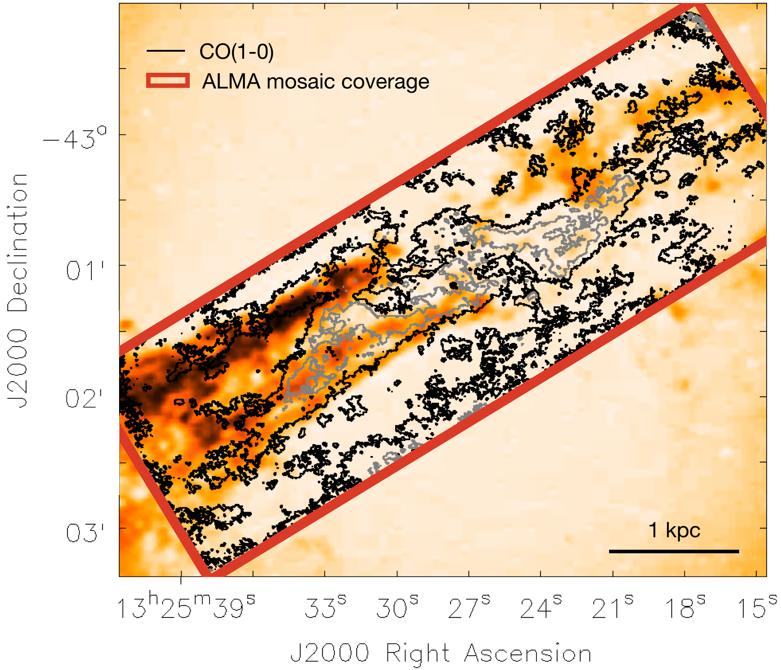
Figure 1.— ALMA band 3 field of view and CO(1–0) integrated intensity contours over the optical image (POSS2-Blue) of NGC 5128 (Centaurus A). Most of the dust lane is covered by the ALMA observations. The contour levels are 3 (black) and 15 $\sigma$ (gray), where $\sigma=0.14$ Jy beam^-1km s^-1. The HPBW of the CO(1–0) map is $1\farcs$39 $\times$ $1\farcs$05 (P.A. = 62°).

The ALMA CO datasets were obtained during 2014 and 2015 as part of program 2013.1.00803.S (P.I. D. Espada). The CO(1–0) dataset consisted of 10 executions: two for the 12m arrays (one extended and one compact configuration dataset), two 7m array, and six TP array datasets. The extended and compact 12m array configurations had longest baseline lengths of 650.3 m and 348.5 m, respectively. The execution IDs, observation dates, time on source and calibrators used are given in Table 1. The total time on source for extended 12m / compact 12m / 7m and TP arrays were 27.8/13.9/57.2/116.2 min.

The spectral setup was designed to observe the CO(1–0) line ($\nu_{\rm rest}$=115.271 GHz). The spectral window in the upper sideband where the line was centered had a bandwidth of $\sim$2450 km s^-1 (937.5 MHz) and a velocity resolution of 1.2 km s^-1  (488.281 kHz). Additional spectral windows were placed at lower frequencies (centre sky frequencies 112.914, 100.999 and 102.699 GHz) using bandwidths of 1875 MHz and resolutions of 31.25 MHz.

Data calibration and imaging were performed using the Common Astronomy Software Applications (CASA; McMullin et al. 2007). We used the packages containing the calibration files provided by the ALMA project. The datasets were delivered using different CASA versions so we opted to perform the data reduction under version 5.1.1 using the scriptForPI.py script provided by ALMA.

The calibration scheme for all the datasets was standard. We carried out phase calibration (using water vapor radiometer data), system temperature calibration, as well as bandpass, phase, amplitude and absolute flux calibration using the calibrators indicated in Table 1. We calibrated each of the interferometric datasets independently and concatenated them after performing line-free continuum subtraction. We checked that visibilities from different elements (extended and compact 12m, 7m, TP arrays) had correct weights after calibration. These weights were calculated inside CASA by taking into account the system temperature ($T_{\rm sys}$) variance, integration time, and antenna diameters.

The single dish data were calibrated in units of antenna temperature ($T_{a}^{*}$) in Kelvin with frequent observations of blank sky (i.e. OFF position). Further residual baseline corrections were done using line-free channels. A scaling factor of 41 Jy K^-1 between $T_{a}^{*}$ and flux density (Kelvin to Jy/beam factor) as obtained by the observatory using a bright quasar for band 3 was applied to the data to convert them to units of Jy/beam.

The CO(1–0) interferometric 12m and 7m data were combined and imaged using the

CLEAN } task with Briggs weighting and robust parameter equal to 0.5.
In this step CASA 5.4 was used as inaccuracies in the primary beam pattern have been recently found in earlier CASA versions.

he spatial resolution of the final images is $1\farcs$39 $\times$ $1\farcs$05 (24.8 $\times$ 18.9 pc), and P.A. = 62°. The resulting data cubes were then combined in CASA with the single dish data cubes using the feathering technique. We generated CO data cubes ranging from $V_{\rm LSRK}=242$ km s^-1 to 820 km s^-1 (Kinematic Local Standard of Rest velocity) and with 2.0 km s^-1 resolution. The combined CO(1–0) data cube is characterized by a typical noise level of 10 mJy beam^-1 for a channel width of 2 km s^-1.

Finally, we produced moment maps. We first smoothed the CO(1–0) datacubes to 20 $\times$ 20 pixels (the size of a pixel is 0$\farcs$2 $\times$ 0$\farcs$2) in the spatial coordinates (Gaussian kernel) and 3 pixels (boxcar) in velocity. Then we obtained masks for regions above a 1$\sigma$ threshold in the CO(1–0) smoothed datacube, which were then applied to the original datacube after visual inspection. Note that at the edges of the mosaic there are regions with lower sensitivity but we exclude them from our analysis. Also, we flagged the absorption line information (e.g. Espada et al. 2010) towards the continuum emission in our analysis. Fig. 2 shows the good agreement between the ALMA single-dish CO(1–0) profile and that obtained from the masked combined CO(1–0) data cube.

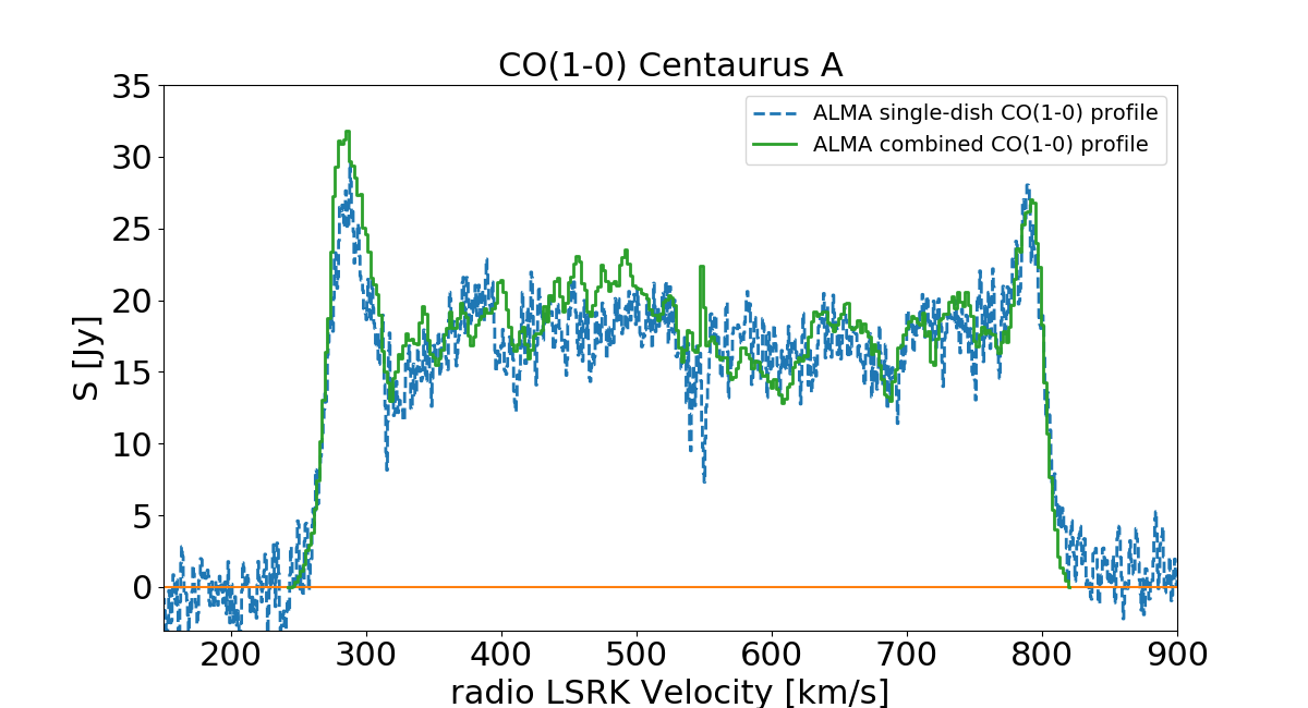
Figure 2.— ALMA single-dish CO(1–0) profile (green full line) compared to the profile obtained from the masked and combined (12m+7m+TP arrays) CO(1–0) data cube (blue dashed line).

2.2. Spitzer 3.6 $\mu$m, 8 $\mu$m, and 24 $\mu$m Archival Data

We compiled Spitzer 3.6 $\mu$m (emission mostly from the old stellar population), 8 $\mu$m (polycyclic aromatic hydrocarbons -PAH, plus warm dust emission), and 24 $\mu$m (warm dust) data from the Spitzer Heritage Archive. The 3.6 $\mu$m and 8 $\mu$m data were obtained with the IRAC instrument (InfraRed Array Camera, Fazio et al. 2004), and the 24 $\mu$m data with the MIPS instrument (Multiband Imaging Photometer for Spitzer, Rieke et al. 2004) onboard the Spitzer Space Telescope (Werner et al. 2004).

The IRAC 3.6 $\mu$m and 8 $\mu$m maps used in this paper were presented in Quillen et al. (2006a) and Quillen et al. (2006b). The angular resolutions (Full Width at Half Maximum, FWHM) are 2$\farcs$2 and 2$\farcs$4, respectively. The MIPS data are post-BCD (higher-level products) processed using the MIPS Data Analysis Tool (Gordon et al. 2005). The FWHM of the MIPS point-spread function (PSF) at 24 $\mu$m is 6$\farcs$0. To remove the backgrounds in all the maps, we first excluded the sources in each image by masking them and then used a sigma clipping technique to robustly estimate the background level which had to be subtracted.

We also removed the old-stellar emission contribution as traced by the 3.6 $\mu$m data from the 8.0 $\mu$m image, assuming that fluxes at 3.6 $\mu$m trace stellar emission only. To do this we followed the recipe $L_{\nu}\ ({\rm PAH})=L_{\nu}\ (8\,\mu{\rm m})-0.232\times L_{\nu}\ (3.6\,\mu{\rm m})$ (Helou et al. 2004; Boquien et al. 2010).

2.3. GALEX FUV Data

The far ultraviolet (FUV, $1350-1750\,\AA$) emission from the young stars of Cen A is investigated through the Galaxy Evolution Explorer (GALEX) (Martin et al. 2005) image, delivered by Gil de Paz et al. (2007), where a description of the reduction procedure is given. We corrected for the Galactic extinction using the conversion factor $A_{\rm FUV}=7.9E(B-V)$ (Gil de Paz et al. 2007) and the Schlafly & Finkbeiner (2011) recalibration of the Schlegel et al. (1998) infrared-based dust map, assuming an $R_{V}=3.1$ Fitzpatrick (1999) reddening law. The image was provided with the background already subtracted and no further treatment has been applied.

3. Molecular Gas

3.1. Molecular Components

We are able to resolve for the first time the molecular component along the dust lane of Cen A into tens of parsec scale molecular clouds thanks to ALMA’s high resolution, sensitivity and high dynamic range. Figs. 3 and 4 show the CO(1–0) integrated-intensity map, velocity field and velocity dispersion map of the molecular disk of Cen A.

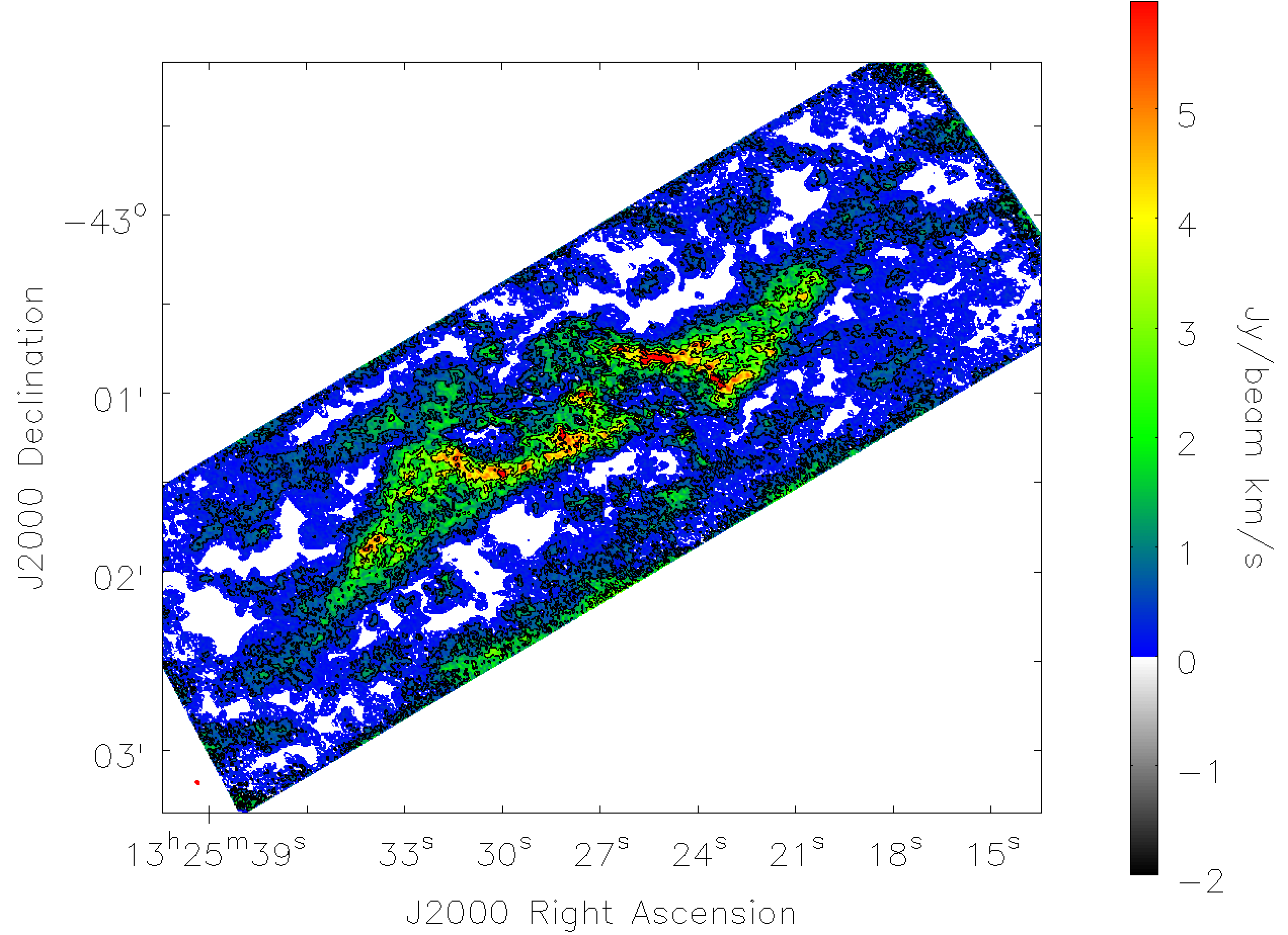
Figure 3.— CO(1–0) integrated-intensity map of the molecular disk of Centaurus A in color scale and contours. The contour levels are 3, 7, 15, 25, and 40 $\sigma$, where $\sigma=0.14$ Jy beam^-1km s^-1. The synthesized beam is shown as a red ellipse in the lower left corner. The HPBW of the CO(1–0) map is $1\farcs$39 $\times$ $1\farcs$05 (P.A. = 62°).

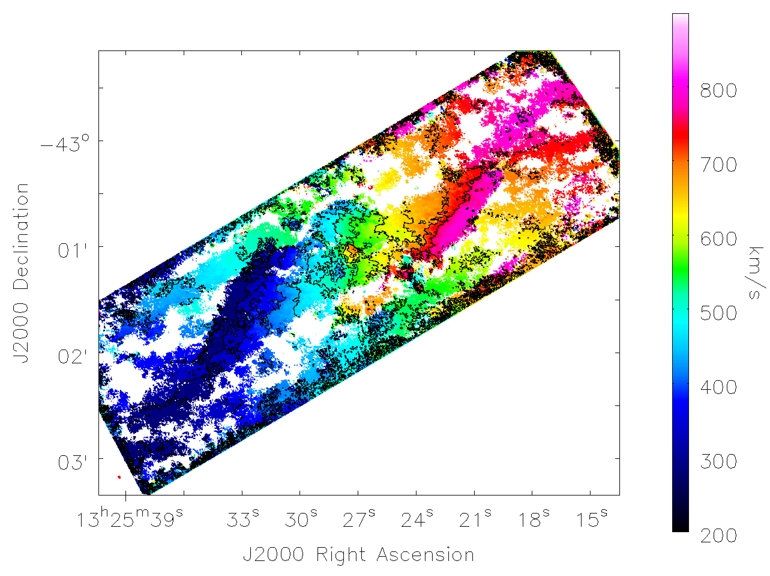
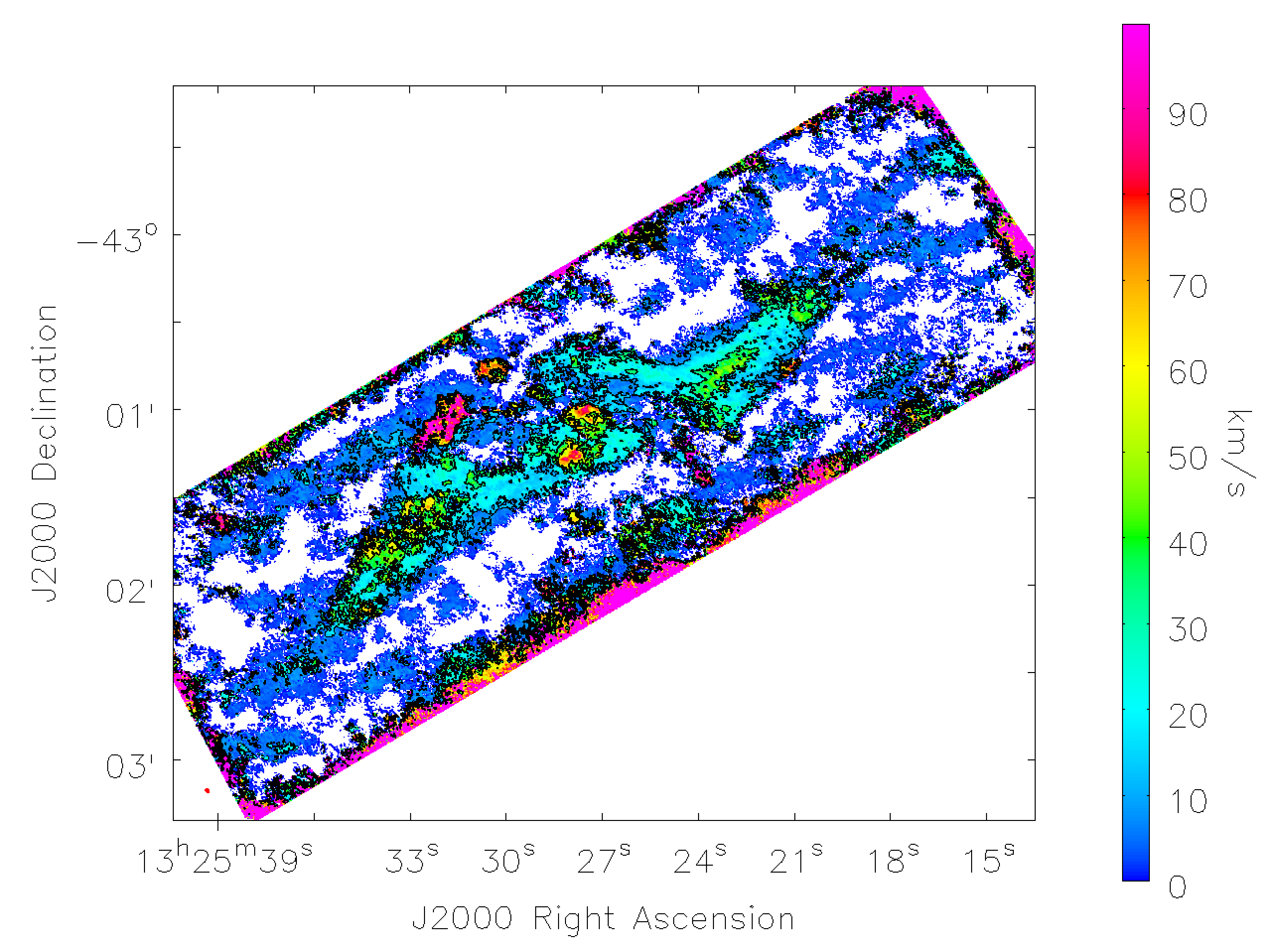
Figure 4.— Top) Intensity-weighted velocity field (moment 1) of the molecular disk of Centaurus A. Contours range from 300 to 800 km s^-1  in bins of 50 km s^-1. Bottom) Velocity dispersion map (moment 2). The contour levels are 10, 30 and 50 km s^-1.

Fig. 5 presents the IRAC 8 $\mu$m over the CO(1–0) contours for comparison. The peculiar morphology seen in the 8 $\mu$m emission (also in the 24 $\mu$m emission) is usually referred to as the ”parallelogram structure” ($\sim$3 kpc in size), which can be partially reproduced by a model of a warped and thin disk seen in projection (Quillen et al. 2006b). This model can match partly the distribution of CO emission, but there are some differences such as the lack of emission on the NE and SW sides of that parallelogram, as well as the curvature of CO(1-0) emission in the form of spiral arms, which are not as clear in the 8 $\mu$m map (Espada et al. 2009, 2012). It is not clear within the warped and thin disk model how the gas of the CND is maintained, since an assumption to reproduce the observed morphologies is the existence of a gap of cold gas and dust from $r$ = 0.2 kpc to 0.8 kpc (Quillen et al. 2006b; Espada et al. 2009).

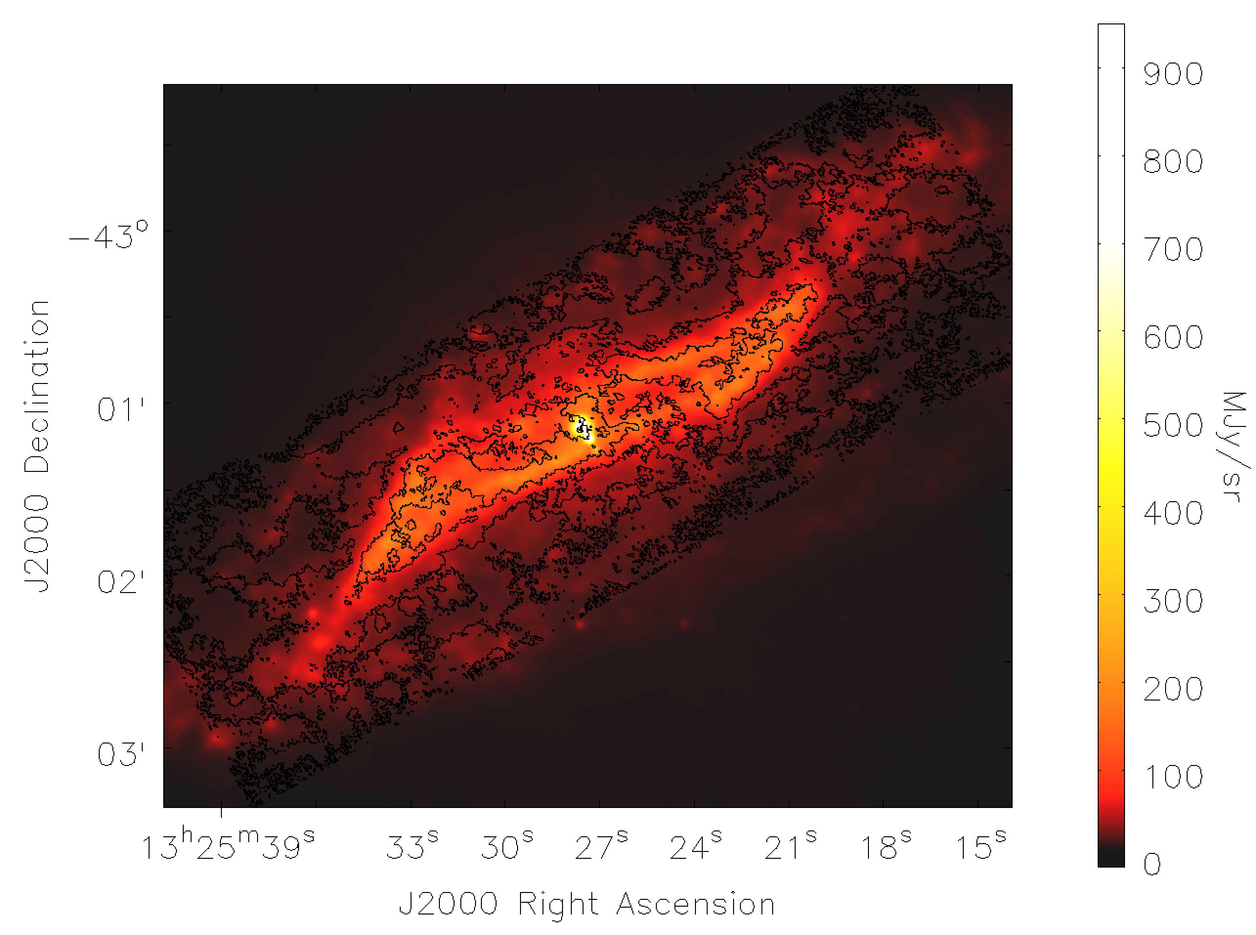
Figure 5.— Spitzer/IRAC 8 $\mu$m map of Centaurus A in color scale shown with the CO(1–0) integrated intensity contours. The contour levels are 1 and 13 $\sigma$, where $\sigma$=0.14 Jy beam^-1km s^-1.

The CO emission is distributed mainly in three distinct regions: the large scale disk, the spiral arm features, and the circumnuclear disk (CND). The distribution and kinematics of the CND and spiral arm regions within the inner 1 kpc are in agreement with previous SubMillimeter Array (SMA) CO(2–1) observations (Espada et al. 2009). The extension of the spiral arms beyond the 1 kpc scale, reported in Espada et al. (2012) using SMA CO(2–1) mosaic observations, is also in agreement, although their field of view was smaller, and the image was less sensitive and characterized by a poorer dynamic range than the one presented here. Besides the main CO components previously observed, the ALMA CO(1–0) map reveals a much shallower and extended molecular disk relative to the previous SMA data, and is composed of multiple filamentary structures covering the dust lane.

The velocity field of Cen A (Fig. 4, top panel) shows that the outer disk component follows the kinematics of the parallelogram disk (i.e. receding side on the NW, and approaching on the SE). However, the different filaments in the outermost regions are kinematically distinct to those in the parallelogram structure. Other peculiar components appear at $\sim$30″ ($\sim$500 pc) to the N and S of the CND, which is probably gas entrained by the jet or associated with the shell-like structure reported by Quillen et al. (2006a). The majority of the clouds in the molecular disk outskirts have velocity dispersions of about $\sim$5 km s^-1 (Fig. 4 bottom), except along the arms and parallelogram structure, where dispersions are $\sim$ 20 km s^-1, and are largest towards the CND. The large velocity dispersions found in the CND are compatible with the results presented in Espada et al. (2017) using the CO(3–2) transition, but as explained there, we note that the velocity dispersions do not exceed $\sim$40 km s^-1. Large velocity dispersions above 40 km s^-1 , in the CND or elsewhere, are usually composed of multiple lines along the line of sight.

3.2. Molecular Gas Mass

First we obtained the CO luminosities, given by:

$$L_{\rm CO(1-0)}=(c^{2}/2k_{B})\,S_{\rm CO(1-0)}\,\nu_{\rm obs}^{-2}\,D_{\rm L}^{2},$$ (1)

where $c$ is the light speed, $k_{B}$ is the Boltzmann constant, $S_{\rm CO}$ is the integrated CO line flux in Jy km s^-1, $\nu_{\rm obs}$ is the observed rest frequency in GHz, 115.271 GHz, and $D_{\rm L}$ is the luminosity distance to the source in Mpc (e.g. Solomon & Vanden Bout 2005). It yields:

$$L_{\rm CO(1-0)}=2445\times S_{\rm CO(1-0)}\,D_{\rm L}^{2}[{\rm K\,\mbox{km s${}^{-1}$}\,pc^{2}}],$$ (2)

and for the case of Cen A we obtain:

$$L_{\rm CO(1-0)}=3.47\times 10^{8}\,{\rm K\,\mbox{km s${}^{-1}$}\,pc}^{2}.$$ (3)

The agreement of this luminosity from the combined dataset with that of the ALMA CO(1–0) single dish data assures that we recover all the flux, as shown also by the profiles in Fig. 2. We also note that single dish data are very important to achieve this. Only 47% of the total flux in the ALMA CO(1–0) single dish data is recovered by the 7m array data.

The luminosity estimates using single dish maps from the literature based on CO(1–0) data (SEST) were found to be 1.73 $\times$ 10⁸ K km s^-1 pc² (corrected by the different distance convention, from 3 to 3.8 Mpc) (Rydbeck et al. 1993; Eckart et al. 1990), lower by about a factor of two than ours. This is partly caused by the larger area covered by our map and to extended emission. A comparison of the integrated flux in our combined map and the pointings along the parallelogram structure in Israel et al. (2014), for a common region encompassing 116″ $\times$ 45″ along a P.A. of 125°, agrees to within 10% (around 4500 Jy km s^-1).

We used as conversion factors between the CO integrated intensity and H₂ column density, $X_{\rm CO}$ $=N_{\rm H_{2}}/I_{\rm CO}$, $X_{\rm CO}$ = 2 $\times$ 10²⁰ cm^-2 (K km s^-1)^-1 for the outer disk, and $X_{\rm CO}$ = 5 $\times$ 10²⁰ cm^-2 (K km s^-1)^-1 for the CND. The factor for the external regions of the disk mass was obtained in Paper II using the virial method (i.e. the comparison of the CO luminosity and virial masses of identified GMCs in the Cen A molecular disk) using the same CO(1–0) data that are presented here. This factor matches the recommended factor for the disk of the Milky Way (e.g. Dame et al. 2001) and other nearby disk galaxies (Bolatto et al. 2013). As for the CND, the larger factor we assume is motivated by the value obtained by Israel et al. (2014) using global single-dish measurements of the CO spectral line energy distribution towards the CND and Large Velocity Gradient (LVG) analysis, $X_{\rm CO}$ = 4 $\times$ 10²⁰ cm^-2 (K km s^-1)^-1. In Paper II, we also confirm a larger factor using the virial method, $X_{\rm CO}$ = $(5\pm 2)\times 10^{20}$ cm^-2(K km s^-1)^-1, in agreement within the uncertainties. In contrast to this result it should be noted that in the circumnuclear regions of starburst galaxies and mergers, as well as in the Galactic center, lower factors are usually found down to a full order of magnitude (e.g. Bolatto et al. 2013). Larger values than the Milky Way disk $X_{\rm CO}$ factor are usually found in low metallicity dwarf galaxies (e.g. Bolatto et al. 2013; Miura et al. 2018). The larger factor is probably caused by high excitation conditions coupled with CO-dark H₂ gas, but it is not likely due to lower metallicities (Paper II).

Finally, we calculated the molecular gas masses as in Bolatto et al. (2013):

$$M_{\rm mol}[{\rm M}_{\odot}]=4.3\times X_{\rm 2}~{}L_{\rm CO(1-0)},$$ (4)

where the factor 1.36 for elements other than hydrogen (Cox 2000) is taken into account, and $X_{\rm 2}$ is the $X_{\rm CO}$ factor normalized to 2 $\times$ $10^{20}$ cm^-2 (K km s^-1)^-1.

The total molecular gas mass in the observed field is $M_{\rm mol}$ $\simeq$ 1.6 $\times$ 10⁹ $M_{\odot}$. The smaller CO luminosity found in the literature as discussed above is reflected in a lower reported molecular gas mass (i.e. $M_{\rm mol}$ = 0.7 $\times$ $10^{9}$ $M_{\odot}$, corrected by different distances, X factors and including the 1.36 factor to account for He), but they are consistent when considering the smaller area covered (i.e. the parallelogram structure). Our CO(1–0) map is sensitive to more extended gas that is beyond the parallelogram structure. In Table 2 we show the derived molecular gas masses of different regions along the disk (i.e. CND, spiral arms, outer disk, etc.).

4. Star Formation Rate

4.1. Validity of using 8 $\mu$m PAH Data as Star Formation Rate Tracer

One of the goals of the present work is to disentangle how the SF activities may vary in the different environments of this galaxy, from the CND close to the AGN to the outermost parts of the molecular disk. We need to reach a high spatial resolution to investigate the KS law locally in Cen A. Approaching the excellent spatial resolution ($\sim 18$ pc) of the ALMA maps for the SFR is not possible but the use of the 8 $\mu$m instead of 24 $\mu$m emission to trace the SFR mitigates this issue by a factor of 2 (Maragkoudakis et al. 2017), and so we chose the 8 $\mu$m band for our analysis because of its higher angular resolution (2$\farcs$4, or 43 pc) compared to that of the 24 $\mu$m data (6$\farcs$0, or 108 pc). Moreover, Elson et al. (2019) showed that the 8 $\mu$m PAH emission is a robust SFR tracer down to physical spatial resolutions of 49 pc.

PAH emission represents generally more than 70% of the 8 $\mu$m emission (Calzetti 2011) and dominates by more than a factor of 100 above the warm dust emission and about a factor of 5 above the stellar continuum (Li & Draine 2001; Dale et al. 2005; Young et al. 2014a). As a consequence, PAH emission (and in particular from the Spitzer 8 $\mu$m band) has been used in the literature to estimate SFR in galaxies (Calzetti et al. 2005; Wu et al. 2005; Pérez-González et al. 2006; Zhu et al. 2008; Pancoast et al. 2010; Calzetti 2011; Kennicutt & Evans 2012; Young et al. 2014a; Cluver et al. 2017; Kokusho et al. 2017; Maragkoudakis et al. 2017; Hall et al. 2018; Elson et al. 2019; Mahajan et al. 2019). Nevertheless, there may be variations from galaxy to galaxy, due to metallicity or different beam filling factors (Engelbracht et al. 2005; Calzetti et al. 2005; Pérez-González et al. 2006; Young et al. 2014a), so it is necessary to assess the validity of the 8 $\mu$m PAH emission as a reliable star formation tracer in Cen A.

To do so, we compared the 8 $\mu$m PAH emission of Cen A to the more robust and widely used 24 $\mu$m emission (Calzetti et al. 2005; Alonso-Herrero et al. 2006; Pérez-González et al. 2006). In Fig. 5 we show the 8 $\mu$m map (with CO(1–0) contours for comparison). We checked the spatial pixel-to-pixel agreement between 8 $\mu$m PAH and 24 $\mu$m fluxes ($F_{\rm 8\,\mu{\rm m}\,PAH}$ and $F_{24\,\mu{\rm m}}$, respectively, in units of MJy sr^-1) in Fig. 6. The 8 $\mu$m PAH map was convolved to the FWHM of the 24 $\mu$m map (6″). We note that in this comparison only data points outside the inner 10″ are shown because of the difficulty to subtract the bright central AGN component in the 24 $\mu$m map, which is worsened by the complex shape of the point spread function. Also we note that we clipped some data points at the low noise level end. We find a very tight (with a correlation coefficient of 0.98) linear correlation which can be expressed as:

$$\log F_{\nu}(\rm 8\,\mu{\rm m}\,PAH)=1.01\times\log F_{\nu}(24\,\mu{\rm m})+0.71\quad.$$ (5)

In Cen A, the linear coefficient against the 24 $\mu$m emission and the very tight correlation over more than two orders of magnitude ensures that the 8 $\mu$m PAH emission is a reliable SFR tracer which, hence, could be linked to the hot dust reprocessing photons from star forming regions (as traced by the 24 $\mu$m emission). Crocker et al. (2011) found that, in a sample of 12 elliptical and lenticular galaxies, the 8 $\mu$m PAH and the 24 $\mu$m emissions yield similar SFR estimates. Therefore the 8 $\mu$m PAH emission will be used to study the spatially resolved KS law in § 5. In the next subsection we will estimate the global SFR in Cen A from a variety of standard SFR tracers.

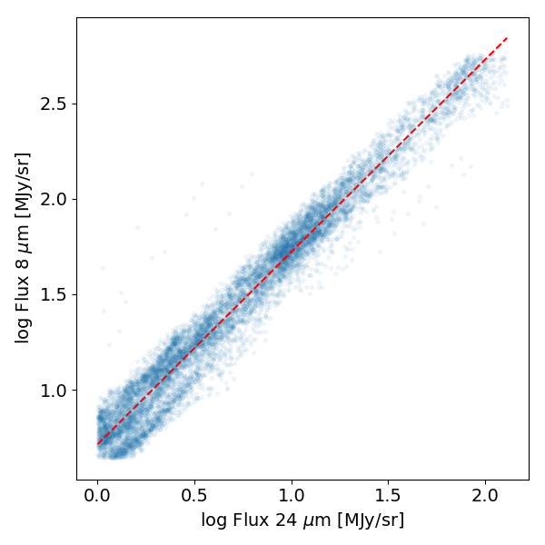
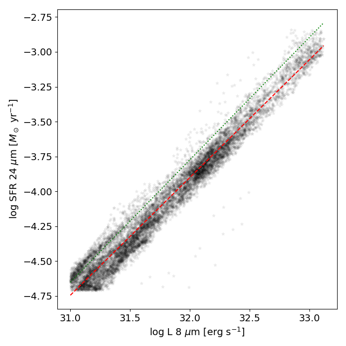
Figure 6.— Left) Correlation between the 8 $\mu$m (PAH) and 24 $\mu$m flux densities in decimal log scale. The (red) dashed line shows the linear fit to the data points, with a slope of 1.01 and correlation coefficient of 0.98. Right) Correlation between the $\Sigma_{\rm SFR}$ (obtained from 24 $\mu$m following the calibration in Calzetti 2013) and the 8 $\mu$m PAH luminosity surface densities ($\Sigma_{L(\rm 8\,\mu{\rm m}\,PAH)}$) in decimal log scale. The (red) dashed line shows the linear fit to the data points. The calibration provided by Boquien et al. (2011) in their Table 2 for M 33 is also shown for comparison as a (green) dotted line.

4.2. Global Star Formation Rate from Various Tracers

A large number of luminosity-to-SFR calibrations can be found in the literature and these conversions can vary by up to $\sim 50$% and create artificial offsets between different works (Kennicutt & Evans 2012), so it is necessary to use homogenized calibrations. In this section, we use the homogenized SF calibrations compiled by Calzetti (2013) (from works by Calzetti et al. 2005, 2007; Kennicutt et al. 2007, 2009; Liu et al. 2011; Hao et al. 2011). All the calibrations make the implicit assumption that the stellar initial mass function (IMF) is constant across all environments and given by the double-power law expression with slope $-1.3$ in the range $0.1-0.5\,M_{\odot}$ and slope $-2.3$ in the range $0.5-120\,M_{\odot}$ (Kroupa 2001) unless noted otherwise.

First, we use a mixed indicator combining the FUV flux from massive stars as well as its dust-obscured counterpart (Calzetti 2013):

$$\begin{split}{\rm SFR_{\rm FUV+24\,\mu{\rm m}}}\ [M_{\odot}\,{\rm yr}^{-1}]=\\ 4.6\cdot 10^{-44}\times[L({\rm FUV})+3.89\cdot L({24\,\mu{\rm m}})]\quad,\end{split}$$ (6)

where $L$ is the luminosity in units of erg s^-1 for a wavelength (or range) $\lambda$. We obtained $L{\rm(FUV)}$ = 4.32 $\times$ 10⁴² erg s^-1 and $L{\rm(24\,\mu{\rm m})}$ = 5.19 $\times$ 10⁴² erg s^-1. This leads to ${\rm SFR_{\rm FUV+24\,\mu{\rm m}}}=1.13\pm 0.09\,M_{\odot}\,{\rm yr}^{-1}$ for Cen A. Second, we use the monochromatic calibration by Rieke et al. (2009) referenced to the same Kroupa (2001) IMF to be consistent with the other calibrations by Calzetti (2013):

$${\rm SFR}_{24\,\mu{\rm m}}\ [M_{\odot}\,{\rm yr}^{-1}]=2.04\times 10^{-43}L({24\,\mu{\rm m}})\ [{\rm erg\,s}^{-1}]\quad,$$ (7)

and it yields ${\rm SFR}_{24\,\mu{\rm m}}=1.06\pm 0.11\,M_{\odot}\,{\rm yr}^{-1}$. Another standard monochromatic calibration, based on the 70 $\mu$m emission (Eq. 22 in Calzetti et al. 2010), reads:

$${\rm SFR}_{70\,\mu{\rm m}}\ [M_{\odot}\,{\rm yr}^{-1}]=5.9\times 10^{-44}L({70\,\mu{\rm m}})\ [{\rm erg\,s}^{-1}]\quad.$$ (8)

We obtain $L{\rm(70\,\mu{\rm m})}$ = 1.95 $\times$ 10⁴³ erg s^-1 (from the 70 $\mu$m flux in Bendo et al. 2012), and it yields ${\rm SFR}_{70\,\mu{\rm m}}=1.15\pm 0.23\,M_{\odot}\,{\rm yr}^{-1}$. Finally, we estimate the total IR (TIR) flux (in W m^-2) in the range $3-1000\,\mu$m, $F({\rm TIR})$, by using the following relation (Dale & Helou 2002; Verley et al. 2010):

$$\begin{split}F({\rm TIR})=10^{-14}\times[19.5\ F_{\nu}(24\,\mu{\rm m})+3.3\ F_{\nu}(70\,\mu{\rm m})\\ +2.6\ F_{\nu}(160\,\mu{\rm m})]\quad,\end{split}$$ (9)

where $F_{\nu}(24\,\mu{\rm m})$, $F_{\nu}(70\,\mu{\rm m})$, and $F_{\nu}(160\,\mu{\rm m})$ are the MIPS flux densities in Jy for Cen A as listed in Table 3 of Bendo et al. (2012). This TIR flux turns into a luminosity of $L(\rm TIR)=1.29\pm 0.16\times 10^{10}\,L_{\odot}$. We can then derive the SFR based on dust-processed stellar light from the TIR luminosity using the following calibration (Calzetti 2013), where the assumptions are a mass range of the stars in the IMF spanning $0.1-100\,M_{\odot}$ and the SF remaining constant during $100$ Myr:

$${\rm SFR_{TIR}}\ [M_{\odot}\,{\rm yr}^{-1}]=2.8\times 10^{-44}\,L({\rm TIR})\ [{\rm erg\,s^{-1}}]\quad,$$ (10)

which leads to SFR_TIR = 1.38 $\pm$ 0.17 $M_{\odot}$ yr^-1 for Cen A. All these estimates of global SFR lead to a consistent result for a SFR in Cen A of about 1 $M_{\odot}$ yr^-1.

The SFRs we have obtained are also in agreement with previous measurements in the literature obtained from IRAS data. The total infrared luminosity was estimated as $L({\rm TIR})$ $\approx$ 2 $L({\rm FIR})=1.12\times 10^{10}\,L_{\odot}$ (Voss & Gilfanov 2006; Marston & Dickens 1988) (corrected to our distance convention distance). Without the contribution of the AGN as estimated by Voss & Gilfanov (2006), then $L({\rm TIR})\approx 9.4\times 10^{9}\,L_{\odot}$. The total SFR is estimated to be $\approx 1\,M_{\odot}\,{\rm yr}^{-1}$ (Colbert et al. 2004; Voss & Gilfanov 2006). Colbert et al. (2004) estimated SFR = $1\,M_{\odot}\,{\rm yr}^{-1}$ (converted to our distance convention) from a combination of $L({\rm FIR})$ and UV luminosity, $L({\rm UV})$, and a conversion factor to convert from $L({\rm FIR+UV})$ to SFR of $5.7\times 10^{-44}$. However, the contribution of the AGN was not subtracted. Voss & Gilfanov (2006) obtained SFR = $1.6\,M_{\odot}\,{\rm yr}^{-1}$ (also converted to our distance convention) from $L({\rm TIR})$ and after subtraction of the AGN contribution. In this estimate, Voss & Gilfanov (2006) used the SFR calibration of Kennicutt (1998), SFR_TIR ($M_{\odot}\,{\rm yr}^{-1})=4.5\times 10^{-44}L({\rm TIR})({\rm erg\,s}^{-1}$). To be able to compare this with our analysis we must convert it to a Kroupa IMF, and therefore we divided it by a factor of 1.59 (Bigiel et al. 2008). Finally, we obtain SFR $\simeq$ 1 M_⊙ yr^-1, which is consistent with all the previously mentioned estimates.

As the 8 $\mu$m PAH emission is so closely tied to the 24 $\mu$m emission (see Fig. 6), we can provide a calibration of the global SFR in Cen A from the 8 $\mu$m PAH emission to reproduce the global SFR obtained from the 24 $\mu$m emission (i.e. $1.06\,M_{\odot}\,{\rm yr}^{-1}$):

$$\begin{split}{\rm SFR}_{\rm 8\mu m\,PAH}\ [M_{\odot}\,{\rm yr}^{-1}]=\\ 6.14\times 10^{-44}L({\rm 8\mu m\,PAH})\ [{\rm erg\,s}^{-1}]\quad.\end{split}$$ (11)

5. Spatially Resolved Kennicutt-Schmidt Star Formation Law

We present the spatially resolved KS SF law using the ALMA CO(1–0) data to derive the molecular gas surface densities ($\Sigma_{\rm mol}$), along with the Spitzer 8 $\mu$m PAH emission. We used a common astrometric grid and we aligned both maps so that there are no artificial offsets. The pixel size in our analysis is 2$\farcs$4 (or 43 pc, i.e. that of the 8 $\mu$m map).

We derived the molecular surface densities, $\Sigma_{\rm mol}$, from the CO(1–0) map presented in § 2.1 and following the convention explained in § 3.2. The map is in units of $M_{\odot}$ pc^-2 and includes the contribution of helium and other heavy elements (a factor 1.36). We estimate that our $\Sigma_{\rm mol}$ map is complete down to surface densities of $\Sigma_{\rm mol}\simeq 4\,M_{\odot}\,{\rm pc}^{-2}$ (corresponding to 3$\sigma$ and a velocity width of 10 km s^-1).

To obtain the SFR surface densities, $\Sigma_{\rm SFR}$, from 8 $\mu$m PAH emission (old-stellar contribution corrected as explained in § 2.2), we take advantage of the very tight correlation between the 24 $\mu$m and the 8 $\mu$m PAH emissions. We estimate the SFR from the 24 $\mu$m emission using the local recipe by Calzetti et al. (2007) calibrated on 220 Hii knots in star forming regions from 33 nearby galaxies. A linear fit to recover the local SFR from 8 $\mu$m PAH emission leads to:

$$\log(\Sigma_{\rm SFR})=0.844\times\log(\Sigma_{L(\rm 8\,\mu{\rm m}\,PAH)})-30.923\quad,$$ (12)

where $\Sigma_{\rm SFR}$ is in units of $M_{\odot}\,{\rm yr}^{-1}\,{\rm kpc}^{-2}$ and $\Sigma_{L(\rm 8\,\mu{\rm m}\,PAH)}$ is the average 8 $\mu$m PAH luminosity surface density in ${\rm erg\,s}^{-1}\,{\rm kpc}^{-2}$.

Similarly, other authors have already reported that the 8 $\mu{\rm m}$ PAH emission correlates with the SFR, but follows a power law with a coefficient slightly less than unity. The sub-linear behaviour has been reported by Calzetti et al. (2005), Pérez-González et al. (2006), Young et al. (2014a), Cluver et al. (2017) and Tomičić et al. (2019), among others. The sub-linear trend is similar to that usually found for the 24 $\mu$m emission (see for example Calzetti et al. 2007; Boquien et al. 2011), as expected because of the strong linear correlation we obtained between the 8 $\mu$m PAH and 24 $\mu$m emissions (Eq. 5). In Fig. 6 (right) we show the result of the linear fit as well as the calibration provided by Boquien et al. (2011) in their Table 2. The two fits have a very similar slope but the Boquien et al. (2011) intercept is slightly higher than the one we find. The recipe provided by Boquien et al. (2011) has been calibrated in the M 33 galaxy, where a relatively high conversion factor is indicative of a rather low dust content (Verley et al. 2009).

Our surface density maps have been corrected by a fixed inclination of 70^∘. This is a good approximation for the average inclination of the disk. However, we note that the disk is likely warped, and the inclination may range from 60 to 120^∘ (Quillen et al. 2010). Fortunately, the uncertain inclination for each pixel and the possible issue of having different components along the line of sight should affect equally both $\Sigma_{\rm mol}$ and $\Sigma_{\rm SFR}$.

5.1. Kennicutt-Schmidt Star Formation Law

We present in Fig. 7 the spatially resolved KS SF law plot (i.e. $\Sigma_{\rm SFR}$ versus $\Sigma_{\rm mol}$) along the dust lane of Centaurus A. The scatter is large, but by visual inspection it is clear that there are two main clusters of data points, one cluster at high $\Sigma_{\rm mol}$ and $\Sigma_{\rm SFR}$, and another centered at $\Sigma_{\rm mol}$ and $\Sigma_{\rm SFR}$ about 1 dex smaller.

We used a machine learning technique to separate the dataset in the $\log\Sigma_{\rm SFR}-\log\Sigma_{\rm mol}$ parameter space (see Fig. 7) into clusters. We first remove the 19 points corresponding to the AGN to focus only on separating the low and high components in this parameter space. We use a Gaussian mixture model (GMM), based on an iterative expectation - maximization algorithm, to extract a mixture of multi-dimensional Gaussian probability distributions that best model our dataset (VanderPlas 2016). To separate our dataset into two components, random initializations are used, and we tested several covariance options (diagonal, spherical, tied, and full covariance matrices). A Bayesian Information Criterion (BIC) selects the best model, which is the one obtained with the full covariance matrix, allowing each cluster to be modeled by an ellipse with arbitrary orientation.

The results of the separation are shown in Fig. 7. This machine learning segregation is able to effectively separate the inner from the outer parts of the galaxy. The highest $\Sigma_{\rm SFR}$ – $\Sigma_{\rm mol}$ cluster corresponds to the CND, arms, and parallelogram regions while the lowest cluster defines the outer disk region. We also use a color/symbol scheme in Fig. 7 (bottom) to separate the data points from the different regions (i.e. CND, arms, parallelogram, and outer disk). Although the separation has a physical meaning regarding regions with high or low SFR/gas surface densities in the CND, arms and outer disk, note that in the parallelogram structure regions the surface densities may artificially be higher because of the projection effect.

The slope of the orthogonal distance regression fit to the data points characterizing the SF law is $N$ = 0.63 (intercept is –2.4). We note however that the scatter is large, there is a trend of decreasing slope for regions at inner radii ( for the CND $N$ = 0.28, and intercept –1.6), and also there might be further uncertainties in the fits due to projection effects, so this result should be taken with caution.

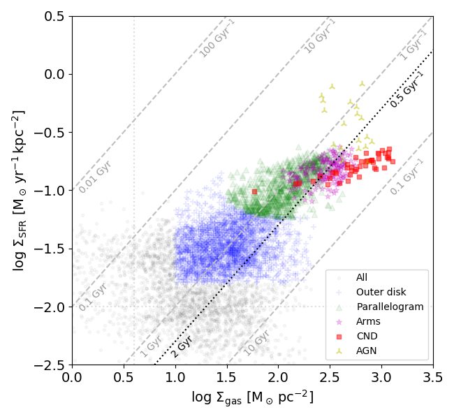
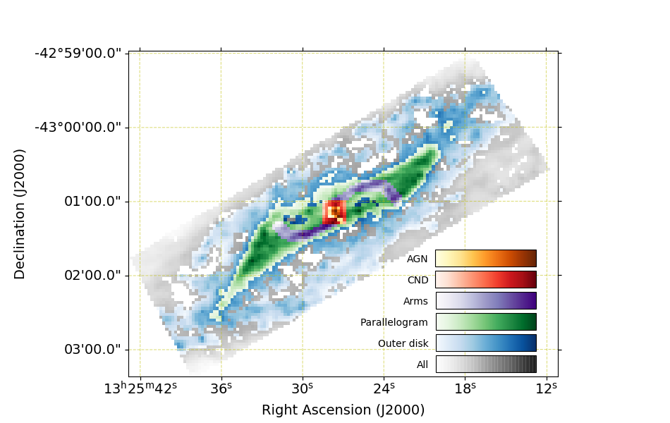
Figure 7.— Top) The Kennicutt-Schmidt star formation law plot of the molecular disk of Centaurus A: star formation rate surface density ($\Sigma_{\rm SFR}$), estimated from 8 $\mu$m PAH emission, as a function of molecular gas surface density ($\Sigma_{\rm mol}$) from the CO(1–0) emission. Each data point corresponds to a 2$\farcs$4 pixel (resolution of the 8 $\mu$m data). Dashed lines indicate constant SFEs at 0.1, 1, 10, and 100 Gyr^-1 (or depletion times 0.01, 0.1, 1, and 10 Gyr). Dotted (vertical and horizontal) lines show the estimated sensitivity limits for $\Sigma_{\rm mol}$ and $\Sigma_{\rm SFR}$. The dotted line at constant SFE 0.5 Gyr^-1 (or depletion time 2 Gyr) is displayed as reference for the SF law of disk galaxies (e.g. Bigiel et al. 2008). The CND (Espada et al. 2009) is marked as red squares, the spiral arms (Espada et al. 2012) as purple star symbols, the parallelogram structure (Quillen et al. 2006b) as green triangles, and the outer disk as blue crosses. Other regions are shown in grey color, and data-points that might be contaminated by the AGN are shown as yellow triangle symbols. Bottom) Scheme showing the main regions color coded as in the upper panel.

5.2. Star Formation Efficiency

In this section we study the Star Formation Efficiency (SFE), defined as the SFR per unit of molecular gas mass, $\Sigma_{\rm SFR}$ / $\Sigma_{\rm mol}$. The depletion time is then defined as the inverse of SFE, $\tau$ = 1/SFE. We find a total molecular gas mass of 1.6 $\times$ 10⁹ $M_{\odot}$ and a global SFR of $\sim$1 $M_{\odot}$ using different recipes, so the SFE is 0.6 Gyr^-1 (or depletion time $\tau=$ 1.5 Gyr), similar to that in spiral galaxies. For reference in the resolved KS plot in Fig. 7 (upper panel), we indicate constant SFE lines, at SFEs 0.1, 1, 10, and 100 Gyr^-1 (or equivalently depletion times $\tau=$ 0.01, 0.1, 1, and 10 Gyr).

Fig. 8 displays the map of the SFE. The SFEs across the disk vary by at least two orders of magnitude from pixel to pixel. We confirm with this plot that the SFEs along the arms and the CND are lower by a factor of 2 to 4 compared to the remaining area, and that higher SFEs are found preferentially in the outskirts of the disk (blue data points in Fig. 7 bottom panel).

In columns 3 to 5 of Table 2 we show the mean, median, and standard deviation of the SFEs obtained from the pixels within the different regions. While the mean SFE in the CND and arms is 0.3 – 0.5 Gyr^-1, in the outer disk it is 1.3 Gyr^-1. Also the standard deviation of the SFEs increases with radius, which likely implies variable physical conditions of molecular gas and star formation activities in the outskirts. This trend is contrary to what is observed in the central regions of other AGNs, as will be discussed in § 6.2.

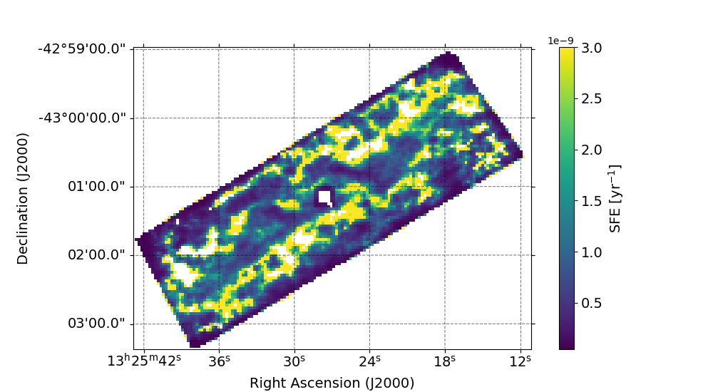
Figure 8.— Pixel-to-pixel map of the star formation efficiency (SFE = $\Sigma_{\rm SFR}$ / $\Sigma_{\rm mol}$) along the dust lane of Cen A.

6. Discussion

6.1. The Fate of Recently Accreted Gas in a Giant Elliptical Galaxy

Cen A is a rare case of a giant elliptical galaxy with a large amount of molecular gas recently accreted and with ongoing SF. In agreement with Young et al. (2009) for other early type galaxies, the bulk of its mid-IR emission can be mostly traced to SF. However, the SF law seems remarkably different to the trends observed for other early type galaxies. Thanks to its recent merger with a gas-rich galaxy, the recent SF history varied substantially compared to other objects of its class. The global SFE ($\sim$ 0.6 Gyr^-1) is compatible within the uncertainties to the average of local star forming galaxies, SFE $\sim$ 1 Gyr^-1 (e.g. Tacconi et al. 2018) found across different galaxy environments (Lisenfeld et al. 2011; Martinez-Badenes et al. 2012).

In the literature it is usually argued that SFEs are either equal or lower in early-type galaxies than the standard relation for late-type galaxies. The derived SFRs and molecular gas surface densities (measured globally) place E/S0 galaxies overlapping the range spanned by disk galaxies although with a larger scatter (Wei et al. 2010; Shapiro et al. 2010). Crocker et al. (2011) find that although 12 E/S0s in the SAURON project lie closely around a constant SFE, as in spiral galaxies, there are some hints of lower SFEs. In fact, it was reported that molecular gas-rich early-type galaxies in the ATLAS3D project have a median SFE of $\sim$0.4 – 0.09  Gyr^-1 (e.g. Davis et al. 2014, 2015), considerably lower than the typical SFEs of $\sim$1 Gyr^-1 in star forming galaxies. It has been suggested that the SF in early types is suppressed due to the stability of the molecular disks against gravitational fragmentation using the Toomre Q test (Davis et al. 2014; Boizelle et al. 2017). This result is supported by hydrodynamic models of Martig et al. (2013), where stars form two to five times less efficiently in early-type galaxies than in spirals. Davis et al. (2015) argue that dynamical effects induced by the minor merger might be responsible for the low SFE values. Recent studies using ALMA observations of some of the most extreme cases in terms of low SFE bulge-dominated galaxies with dust lanes confirmed that SFE ranges from 0.002 – 0.04 Gyr^-1 (van de Voort et al. 2018). However, Kokusho et al. (2017) find that most of the ATLAS3D local early type galaxies follow the same SF law as local later type star-forming galaxies. Contrary to recent results suggesting slightly lower SFEs, they claim that this is directly related to the somewhat lower SFRs derived in those works. They note however that there is evidence that early type galaxies whose cold gas has an external origin (kinematically misaligned gas with respect to stars) have more varied SFEs, which may suggest a more bursty and variable recent SF history. This might be the case for Cen A.

A parameter that is crucial to understand the different claims regarding the SFE in early-type galaxies is the stellar mass. In Cen A the stellar mass is $M_{\star}$ = 10¹¹ $M_{\odot}$ (Kormendy & Ho 2013). This value is within the range of the early-type galaxy sample with recent minor mergers studied by Davis et al. (2015). About 80% of their low mass E/S0s ($M_{\star}$ $<$ 4 $\times$ 10¹⁰ $M_{\odot}$) present high SFEs (above the KS law), and are usually star forming (i.e. blue sequence) objects (Wei et al. 2010). The fraction of E/S0s that are star forming increases with decreasing stellar mass (Kannappan et al. 2009). Indeed, Cen A’s stellar mass is close to the ”shutdown mass” (i.e. mass at which blue-sequence E/S0s first emerge, and above which nearly all galaxies are generally old and red) for blue sequence early type objects, $M_{\rm s}$ $\sim$ 1 – 2 $\times$ 10¹¹ $M_{\odot}$, which only a minority (2%) of E/S0s exceed (Kannappan et al. 2009). So in summary Cen A is at the massive end where it is rare to find a star-forming elliptical. It is therefore likely that it is mostly by accretion events that such an object can exist.

Next we put the case of Cen A in the context of previous works where the SFEs were found to be either equal or lower than the standard values of spiral galaxies. Because Cen A recently accreted material, it would match the selection criteria of galaxies in the samples of Davis et al. (2015) and van de Voort et al. (2018). Indeed they focus on a sample of bulge-dominated galaxies with large dust lanes and with signs of a recent minor merger. In these works it is argued that the SFE is suppressed as a result of dynamical effects. How can we reconcile the apparent contradiction of Cen A presenting a nearly standard SFE similar to star forming galaxies? This can be due to different impact parameters of the merger, merged galaxy properties (such as mass and gas fraction), and the dynamical relaxation time. At any rate, the case of Cen A shows that the SFE is not always suppressed in early-type galaxies after gas-rich minor mergers. ALMA observations of the elliptical and radio jet galaxy NGC 3557 have recently shown that its molecular disk within the inner hundreds of parsec presents a global SFE that may be compatible with the standard relation in spiral star-forming galaxies too (Vila-Vilaro et al. 2019).

In about 1 Gyr, objects like Cen A may look more similar to other objects of its class (i.e. giant elliptical galaxies without much molecular gas and with low SFEs). A fast evolutionary sequence may be playing a role, which would explain why only a minority of massive early type galaxies are in the blue sequence even though they are in high galaxy density environments where accretion events are relatively frequent. The molecular gas will be exhausted preferentially in the external regions. The SFE is higher in the outskirts by a factor of four than in the central regions of Cen A so it will be consumed faster. In addition, the gas will be either driven to the central regions, or destroyed because of a lack of self-shielding to massive SF combined with the hot environmental conditions within the elliptical galaxy (i.e. a hot ISM thermally radiating at X-rays, Henkel & Wiklind 1997). Dense gas that is stable against collapse due to inflowing motions, shear, and/or excess of shocks/turbulence will remain, preferentially in compact components or filamentary structures within the stellar component, which is the result observed in other massive elliptical galaxies.

6.2. The Low SFE in the CND of Cen A: A Comparison with Low Luminosity AGNs and Nuclear Starbursts

For the amount of molecular gas in the CND, the SFR is comparatively smaller than that found in other regions. The mean SFE in the CND is just about $\sim 0.3$ Gyr^-1 at 40 pc scales, four times smaller than in the outer regions (see § 5.2). Using photon-dominated region (PDR) modeling of the neutral and ionized gas from the far-infrared lines, Israel et al. (2017) claimed that because the radiation field in the CND is weaker by an order of magnitude than in the extended disk, no significant SF in the CND is required. The radiation field strength could be explained just by the radiation coming from the stellar component of the extended disk. We do find that the SFR in the CND is small but not negligible. We note that this SFR is a lower limit because we have excluded pixels close to the AGN that may be contaminated by it, but the SFE we quote is representative for the outer ($r$ = 100 – 200 pc) regions of the CND.

A source of uncertainty in the deduced low SFE of the CND is the $X_{\rm CO}$ factor used to calculate the molecular gas mass. For the CND we used a conversion factor $X_{\rm CO}$ = $5\times 10^{20}$ cm^-2(K km s^-1)^-1, while for the rest of the disk we applied $2\times 10^{20}$ cm^-2(K km s^-1)^-1. However, a different $X_{\rm CO}$ in the central regions is supported by an analysis in Israel et al. (2014) using LVG modeling on CO spectral line energy distribution, and Paper II using the virial method. These are independent methods so this result is likely robust. Moreover, in Paper II we found a gradual increase of $X_{\rm CO}$ towards inner radii. We note that $X_{\rm CO}$ is driven by metallicity in the low metallicity regime, but in the case of Cen A metallicity across the molecular disk (including the CND) is $\sim 0.75$ $Z_{\odot}$ and relatively constant.

The SFEs are also relatively constant at 1 – 2 Gyr^-1 along galactocentric radii on kpc scales (Leroy et al. 2008, 2013; Muraoka et al. 2019). However, Leroy et al. (2013) systematically found higher SFEs for a given $X_{\rm CO}$ in the inner kpc of a sample of 30 nearby disk galaxies that show nuclear molecular gas concentrations, including AGN and nuclear starbursts, but not galaxy-wide starbursts. Our finding of lower SFEs in the CND compared to the outer regions of Cen A contradicts this. Since $X_{\rm CO}$ is typically smaller by a factor of 2 below the galaxy mean on average close to their nuclei (Sandstrom et al. 2013), and in some cases 5 –10 times below the standard galaxy disk value, the resulting SFEs are higher than when assuming a constant $X_{\rm CO}$.

A direct comparison of SFEs between different objects requires the use of similar spatial scales. Using ALMA CO(2–1) maps of 14 disk galaxies, Utomo et al. (2018) found that on 120 pc scales SFEs range from 0.43 – 1.65 Gyr^-1, similar to the range we see for the different regions in Cen A, from SFE = 0.3 – 0.5 Gyr^-1 in the CND/arms region, to SFE = 1.3 Gyr^-1 in the outer disk. Casasola et al. (2015) studied the central regions (from 20 to 200 pc) of a sample of four galaxies possessing low luminosity AGNs, i.e. Seyfert and LINER nuclei, and they found that they were characterized by higher SFEs than the standard value for disk galaxies (adopting a common $X_{\rm CO}$ factor $2.2\times 10^{20}$ cm^-2(K km s^-1)^-1), with a behaviour that is in between galaxy-wide starburst systems and more quiescent galaxies. The SFR and gas surface densities of the central regions of these objects are comparable to those in the CND of Cen A, ranging from $\sim$ 0.01 to 1 $M_{\odot}$ yr^-1 kpc^-2 and $\sim$ 10² to 10³ $M_{\odot}$ pc^-2, respectively. Possible causes for the lower SFEs in the CND of Cen A are stronger shear motions and shocks. Also, the more continuous period of AGN feedback in the case of Cen A than in other AGNs may be responsible for the observed differences. However, we also note that other late-type AGN galaxies with low SFEs towards the circumnuclear regions also exist, such as in the inner spiral regions of NGC 1068 (Tsai et al. 2012). In our Galactic centre the current SFR per unit mass of dense gas was also found to be an order of magnitude smaller than in the disk (Longmore et al. 2013).

7. Summary

High angular/spectral resolution, sensitivity, and dynamic range ALMA CO(1–0) data is presented for the nearest giant elliptical and radio galaxy, Centaurus A (NGC 5128). We combined ALMA 12m, 7m and TP array data in order to recover the flux at all spatial scales. We performed a Kennicutt-Schmidt Star Formation law analysis at GMC scales ($\sim$ 40 pc) using ALMA CO(1–0) data for the molecular gas and archival Spitzer mid-IR data as a tracer of the SFR. We exclude from our analysis regions where the star formation rate (SFR) tracer is contaminated by emission from the active galactic nucleus (AGN). Our main results can be summarized as follows:

1. We revealed several filamentary molecular components beyond the previously known main molecular components (circumnuclear disk -CND-, arms, parallelogram structure; Espada et al. 2009, 2012) in the outer regions of the molecular disk, extending up to a radius of $\sim$ 3 kpc. There is a good correlation with the mid-IR continuum emission.

2. We obtained a total molecular gas mass across the dust lane of Cen A based on CO(1–0) emission of 1.6 $\times$ 10⁹ $M_{\odot}$. This is larger than previously reported because of a larger field of view and better sensitivity to extended flux in our observations. We use a conversion factor $X_{\rm CO}$ = $2\times 10^{20}$ cm^-2(K km s^-1)^-1, except for the CND where we use $5\times 10^{20}$ cm^-2(K km s^-1)^-1 as recommended in Miura et al. (2019, Paper II) using the virial method. This is compatible with Israel et al. (2014) using multi-transition analysis and LVG (Large Velocity Gradient) modeling.

3. The global SFR is $\simeq$ 1 $M_{\odot}$ yr^-1 based on Spitzer mid-IR data (and GALEX FUV data), also consistent with previous estimates based on IRAS data. Therefore the global star formation efficiency (SFE) is 0.6 Gyr^-1 (depletion time $\tau=$ 1.5 Gyr), similar to that in star forming galaxies ($\sim$ 1 Gyr, e.g. Tacconi et al. 2018).

4. The molecular gas and SFR surface densities at 40 pc scale range from $\Sigma_{\rm mol}$ = 4 to 10³ M_☉  pc^-2 and $\Sigma_{\rm SFR}$ = 10^-2 to 10^-0.7 M_☉  yr^-1 kpc^-2, similar to the typical ranges in nearby disk galaxies. Although the scatter is large, the slope of the orthogonal distance regression fit is $N$ = 0.63 (intercept is –2.4) and there is a trend of decreasing slope for regions at inner radii. For the CND $N$ = 0.28, and the intercept is –1.6.

5. In the pixel-to-pixel (40 pc) analysis we see that the mean/median SFEs (and standard deviations) for the different regions increase as a function of radius. The CND presents on average a lower SFE (0.3 Gyr^-1) by a factor of four than that in the outskirts of the molecular disk. This is compatible with the range (0.4 – 1.6 Gyr^-1) observed in nearby disk galaxies on 120 pc scales (Utomo et al. 2018).

6. The global SFE is in agreement with those found for other early-type galaxies in the literature that show similar SFEs to disk galaxies (e.g. Kokusho et al. 2017). However, this is not consistent with studies reporting lower SFEs for a sample of bulge-dominated galaxies with large dust lanes and with signs of a recent minor merger, properties that match those of Cen A (e.g. Davis et al. 2015; van de Voort et al. 2018). Cen A shows that not in all cases is the SFE suppressed in early-type galaxies after gas-rich minor mergers. However, regions with low SFE can also be found within the molecular disk of Cen A. The best example is the CND of Cen A where strong shear and shocks together with AGN activity (Espada et al. 2017) are likely important mechanisms to prevent SF.

7. Giant ellipticals ($M_{\star}$ $\geq$ 10¹¹ $M_{\odot}$) like Cen A with a large amount of molecular gas (likely of external origin), extending $\sim$3 kpc in radius, and with ongoing SF comparable to that of a spiral galaxy are rare. This can be partly explained because molecular gas can be exhausted by SF in $\sim$1 Gyr and destroyed by its feedback preferentially in those regions with lower gas densities (i.e. the outskirts of the disk) where self-shielding is limited. This is to be combined with the harsh environmental conditions within the elliptical galaxies, where a hot ISM is present thermally radiating at X-rays. At a later stage, only dense molecular gas stable against collapse due to dynamical effects will remain, usually in the form of compact components around the center or filamentary structures. These would be the resulting molecular components with low star forming efficiency usually observed in other massive ellipticals.

8. The low SFE in the CND of Centaurus A is also in contrast to that of low luminosity AGNs and nuclear starbursts, where SFEs are $\sim$1.25 times those of their corresponding disk region (Leroy et al. 2013). This can be partly a consequence of the high $X_{\rm CO}$ towards the CND of Cen A (Paper II, Israel et al. 2014), which is opposite to the trend observed on average close to the nuclei of AGN/nuclear starbursts by factors from 2 – 10 (Sandstrom et al. 2013). Possible causes are stronger shear motions, shocks and the more continuous period of AGN feedback in the case of Cen A than in low luminosity AGNs and nuclear starbursts.

Table 1Summary of ALMA CO(1–0) Data

Execution Block IDs	Observation date	Time on Source (min)	Configuration	Calibrators
CO(1–0)
uid://A002/X83dbe6/X9ec	2014-06-11	27.8	ext. 12m array	Ceres, J1427-4206, J1321-4342
uid://A002/X95e355/X1ac1	2014-12-06	13.9	comp. 12m array	Titan, J1427-4206, J1254-4424
uid://A002/X83f101/X165	2014-06-12	57.2	7m array	Mars, J1427-4206, J1321-4342
uid://A002/X83f101/X49a	2014-06-11	57.2	”	Mars, J1427-4206, J1321-4342
uid://A002/X99b784/Xc88	2015-01-16	19.4	TP array
uid://A002/X99c183/X33fa	2015-01-17	19.4	”
uid://A002/X99c183/X37b2	2015-01-17	19.4	”
uid://A002/X99c183/X3a1e	2015-01-17	19.4	”
uid://A002/X9d9aa5/X2058	2015-04-08	19.4	”
uid://A002/X9d9aa5/X23d7	2015-04-08	19.4	”

Table 2Molecular gas masses and SFEs in different regions of the disk of Centaurus A

Region	$M_{\rm mol}$[108 $M_{\odot}$]	mean SFE [Gyr-1]	Median SFE [Gyr-1]	stddev SFE [Gyr-1]
CND	1.65	0.32	0.26	0.24
Arms	2.72	0.55	0.49	0.21
Parallelogram	5.99	1.02	0.88	0.52
Outer disk	5.65	1.29	1.05	0.93

References

- Alonso-Herrero et al. (2006) Alonso-Herrero, A., Rieke, G. H., Rieke, M. J., et al. 2006, ApJ, 650, 835
- Astropy Collaboration et al. (2013) Astropy Collaboration, Robitaille, T. P., Tollerud, E. J., et al. 2013, A&A, 558, doi:10.1051/0004-6361/201322068
- Bendo et al. (2012) Bendo, G. J., Galliano, F., & Madden, S. C. 2012, MNRAS, 423, 197
- Bigiel et al. (2008) Bigiel, F., Leroy, A., Walter, F., et al. 2008, AJ, 136, 2846
- Boizelle et al. (2017) Boizelle, B. D., Barth, A. J., Darling, J., et al. 2017, ApJ, 845, 170
- Bolatto et al. (2013) Bolatto, A. D., Wolfire, M., & Leroy, A. K. 2013, ARA&A, 51, 207
- Boquien et al. (2010) Boquien, M., Bendo, G., Calzetti, D., et al. 2010, ApJ, 713, 626
- Boquien et al. (2011) Boquien, M., Calzetti, D., Combes, F., et al. 2011, AJ, 142, 111
- Calzetti (2011) Calzetti, D. 2011, in EAS Publications Series, Vol. 46, EAS Publications Series, ed. C. Joblin & A. G. G. M. Tielens, 133–141
- Calzetti (2013) Calzetti, D. 2013, Star Formation Rate Indicators, ed. J. Falcón-Barroso & J. H. Knapen, 419
- Calzetti et al. (2005) Calzetti, D., Kennicutt, R. C., J., Bianchi, L., et al. 2005, ApJ, 633, 871
- Calzetti et al. (2007) Calzetti, D., Kennicutt, R. C., Engelbracht, C. W., et al. 2007, ApJ, 666, 870
- Calzetti et al. (2010) Calzetti, D., Wu, S.-Y., Hong, S., et al. 2010, ApJ, 714, 1256
- Casasola et al. (2015) Casasola, V., Hunt, L., Combes, F., & García-Burillo, S. 2015, A&A, 577, A135
- Cluver et al. (2017) Cluver, M. E., Jarrett, T. H., Dale, D. A., et al. 2017, ApJ, 850, 68
- Colbert et al. (2004) Colbert, E. J. M., Heckman, T. M., Ptak, A. F., Strickland, D. K., & Weaver, K. A. 2004, ApJ, 602, 231
- Cox (2000) Cox, A. N. 2000, Allen’s astrophysical quantities
- Crocker et al. (2011) Crocker, A. F., Bureau, M., Young, L. M., & Combes, F. 2011, MNRAS, 410, 1197
- Daddi et al. (2010) Daddi, E., Elbaz, D., Walter, F., et al. 2010, ApJ, 714, L118
- Dale & Helou (2002) Dale, D. A., & Helou, G. 2002, ApJ, 576, 159
- Dale et al. (2005) Dale, D. A., Bendo, G. J., Engelbracht, C. W., et al. 2005, ApJ, 633, 857
- Dame et al. (2001) Dame, T. M., Hartmann, D., & Thaddeus, P. 2001, ApJ, 547, 792
- Davis et al. (2014) Davis, T. A., Young, L. M., Crocker, A. F., et al. 2014, MNRAS, 444, 3427
- Davis et al. (2015) Davis, T. A., Rowlands, K., Allison, J. R., et al. 2015, MNRAS, 449, 3503
- Eckart et al. (1990) Eckart, A., Cameron, M., Rothermel, H., et al. 1990, ApJ, 363, 451
- Elson et al. (2019) Elson, E. C., Kam, S. Z., Chemin, L., Carignan, C., & Jarrett, T. H. 2019, MNRAS, 483, 931
- Engelbracht et al. (2005) Engelbracht, C. W., Gordon, K. D., Rieke, G. H., et al. 2005, ApJ, 628, L29
- Espada et al. (2012) Espada, D., Matsushita, S., Peck, A. B., et al. 2012, ApJ, 756, L10
- Espada et al. (2009) Espada, D., Matsushita, S., Peck, A., et al. 2009, ApJ, 695, 116
- Espada et al. (2010) Espada, D., Peck, A. B., Matsushita, S., et al. 2010, ApJ, 720, 666
- Espada et al. (2017) Espada, D., Matsushita, S., Miura, R. E., et al. 2017, ApJ, 843, 136
- Fazio et al. (2004) Fazio, G. G., Hora, J. L., Allen, L. E., et al. 2004, The Astrophysical Journal Supplement Series, 154, 10
- Fitzpatrick (1999) Fitzpatrick, E. L. 1999, PASP, 111, 63
- Gil de Paz et al. (2007) Gil de Paz, A., Boissier, S., Madore, B. F., et al. 2007, ApJS, 173, 185
- Gordon et al. (2005) Gordon, K. D., Rieke, G. H., Engelbracht, C. W., et al. 2005, PASP, 117, 503
- Hall et al. (2018) Hall, C., Courteau, S., Jarrett, T., et al. 2018, ApJ, 865, 154
- Hao et al. (2011) Hao, C.-N., Kennicutt, R. C., Johnson, B. D., et al. 2011, ApJ, 741, 124
- Harris et al. (2010) Harris, G. L. H., Rejkuba, M., & Harris, W. E. 2010, PASA, 27, 457
- Hawarden et al. (1993) Hawarden, T. G., Sandell, G., Matthews, H. E., et al. 1993, MNRAS, 260, 844
- Helou et al. (2004) Helou, G., Roussel, H., Appleton, P., et al. 2004, The Astrophysical Journal Supplement Series, 154, 253
- Henkel & Wiklind (1997) Henkel, C., & Wiklind, T. 1997, Space Sci. Rev., 81, 1
- Hunter (2007) Hunter, J. D. 2007, Computing In Science & Engineering, 9, 90
- Israel et al. (2017) Israel, F. P., Güsten, R., Meijerink, R., Requena-Torres, M. A., & Stutzki, J. 2017, A&A, 599, A53
- Israel et al. (2014) Israel, F. P., Güsten, R., Meijerink, R., et al. 2014, A&A, 562, A96
- Kannappan et al. (2009) Kannappan, S. J., Guie, J. M., & Baker, A. J. 2009, AJ, 138, 579
- Kennicutt (1998) Kennicutt, Robert C., J. 1998, Annual Review of Astronomy and Astrophysics, 36, 189
- Kennicutt et al. (2009) Kennicutt, Robert C., J., Hao, C.-N., Calzetti, D., et al. 2009, ApJ, 703, 1672
- Kennicutt & Evans (2012) Kennicutt, R. C., & Evans, N. J. 2012, ARA&A, 50, 531
- Kennicutt et al. (2007) Kennicutt, Jr., R. C., Calzetti, D., Walter, F., et al. 2007, ApJ, 671, 333
- Kohno et al. (2002) Kohno, K., Tosaki, T., Matsushita, S., et al. 2002, Publications of the Astronomical Society of Japan, 54, 541
- Kokusho et al. (2017) Kokusho, T., Kaneda, H., Bureau, M., et al. 2017, A&A, 605, A74
- Kormendy & Ho (2013) Kormendy, J., & Ho, L. C. 2013, Annual Review of Astronomy and Astrophysics, 51, 511
- Kroupa (2001) Kroupa, P. 2001, MNRAS, 322, 231
- Leeuw et al. (2002) Leeuw, L. L., Hawarden, T. G., Matthews, H. E., Robson, E. I., & Eckart, A. 2002, ApJ, 565, 131
- Leroy et al. (2008) Leroy, A. K., Walter, F., Brinks, E., et al. 2008, AJ, 136, 2782
- Leroy et al. (2013) Leroy, A. K., Walter, F., Sandstrom, K., et al. 2013, AJ, 146, 19
- Li & Draine (2001) Li, A., & Draine, B. T. 2001, ApJ, 554, 778
- Lisenfeld et al. (2011) Lisenfeld, U., Espada, D., Verdes-Montenegro, L., et al. 2011, A&A, 534, A102
- Liszt (2001) Liszt, H. 2001, A&A, 371, 865
- Liu et al. (2011) Liu, G., Koda, J., Calzetti, D., Fukuhara, M., & Momose, R. 2011, ApJ, 735, 63
- Longmore et al. (2013) Longmore, S. N., Bally, J., Testi, L., et al. 2013, MNRAS, 429, 987
- Mahajan et al. (2019) Mahajan, S., Ashby, M. L. N., Willner, S. P., et al. 2019, MNRAS, 482, 560
- Maragkoudakis et al. (2017) Maragkoudakis, A., Zezas, A., Ashby, M. L. N., & Willner, S. P. 2017, MNRAS, 466, 1192
- Marston & Dickens (1988) Marston, A. P., & Dickens, R. J. 1988, A&A, 193, 27
- Martig et al. (2013) Martig, M., Crocker, A. F., Bournaud, F., et al. 2013, MNRAS, 432, 1914
- Martin et al. (2005) Martin, D. C., Fanson, J., Schiminovich, D., et al. 2005, ApJ, 619, L1
- Martinez-Badenes et al. (2012) Martinez-Badenes, V., Lisenfeld, U., Espada, D., et al. 2012, A&A, 540, A96
- McCoy et al. (2017) McCoy, M., Ott, J., Meier, D. S., et al. 2017, ApJ, 851, 76
- McMullin et al. (2007) McMullin, J. P., Waters, B., Schiebel, D., Young, W., & Golap, K. 2007, in Astronomical Society of the Pacific Conference Series, Vol. 376, Astronomical Data Analysis Software and Systems XVI, ed. R. A. Shaw, F. Hill, & D. J. Bell, 127
- Mirabel et al. (1999) Mirabel, I. F., Laurent, O., Sanders, D. B., et al. 1999, A&A, 341, 667
- Miura et al. (2019) Miura, R. E., Espada, D., & et al. 2019, ApJ, (Paper II)
- Miura et al. (2018) Miura, R. E., Espada, D., Hirota, A., et al. 2018, ApJ, 864, 120
- Miura et al. (2014) Miura, R. E., Kohno, K., Tosaki, T., et al. 2014, ApJ, 788, 167
- Muraoka et al. (2019) Muraoka, K., Sorai, K., Miyamoto, Y., et al. 2019, Publications of the Astronomical Society of Japan, 27
- Nicholson et al. (1992) Nicholson, R. A., Bland-Hawthorn, J., & Taylor, K. 1992, ApJ, 387, 503
- Onodera et al. (2010) Onodera, S., Kuno, N., Tosaki, T., et al. 2010, ApJ, 722, L127
- Pancoast et al. (2010) Pancoast, A., Sajina, A., Lacy, M., Noriega-Crespo, A., & Rho, J. 2010, ApJ, 723, 530
- Parkin et al. (2012) Parkin, T. J., Wilson, C. D., Foyle, K., et al. 2012, MNRAS, 422, 2291
- Parkin et al. (2014) Parkin, T. J., Wilson, C. D., Schirm, M. R. P., et al. 2014, ApJ, 787, 16
- Pedregosa et al. (2011) Pedregosa, F., Varoquaux, G., Gramfort, A., et al. 2011, Journal of Machine Learning Research, 12, 2825
- Perez & Granger (2007) Perez, F., & Granger, B. E. 2007, Computing in Science and Engineering, 9, 21
- Pérez-González et al. (2006) Pérez-González, P. G., Kennicutt, Robert C., J., Gordon, K. D., et al. 2006, ApJ, 648, 987
- Phillips et al. (1987) Phillips, T. G., Ellison, B. N., Keene, J. B., et al. 1987, ApJ, 322, L73
- Quillen et al. (2006a) Quillen, A. C., Bland-Hawthorn, J., Brookes, M. H., et al. 2006a, ApJ, 641, L29
- Quillen et al. (2006b) Quillen, A. C., Brookes, M. H., Keene, J., et al. 2006b, ApJ, 645, 1092
- Quillen et al. (1993) Quillen, A. C., Graham, J. R., & Frogel, J. A. 1993, ApJ, 412, 550
- Quillen et al. (2010) Quillen, A. C., Neumayer, N., Oosterloo, T., & Espada, D. 2010, PASA, 27, 396
- Rieke et al. (2009) Rieke, G. H., Alonso-Herrero, A., Weiner, B. J., et al. 2009, ApJ, 692, 556
- Rieke et al. (2004) Rieke, G. H., Young, E. T., Cadien, J., et al. 2004, in Proc. SPIE, Vol. 5487, Optical, Infrared, and Millimeter Space Telescopes, ed. J. C. Mather, 50–61
- Robitaille & Bressert (2012) Robitaille, T., & Bressert, E. 2012, APLpy: Astronomical Plotting Library in Python, Astrophysics Source Code Library, , , ascl:1208.017
- Rydbeck et al. (1993) Rydbeck, G., Wiklind, T., Cameron, M., et al. 1993, A&A, 270, L13
- Sandstrom et al. (2013) Sandstrom, K. M., Leroy, A. K., Walter, F., et al. 2013, ApJ, 777, 5
- Schlafly & Finkbeiner (2011) Schlafly, E. F., & Finkbeiner, D. P. 2011, ApJ, 737, 103
- Schlegel et al. (1998) Schlegel, D. J., Finkbeiner, D. P., & Davis, M. 1998, ApJ, 500, 525
- Schmidt (1959) Schmidt, M. 1959, ApJ, 129, 243
- Shapiro et al. (2010) Shapiro, K. L., Falcón-Barroso, J., van de Ven, G., et al. 2010, MNRAS, 402, 2140
- Solomon & Vanden Bout (2005) Solomon, P. M., & Vanden Bout, P. A. 2005, ARA&A, 43, 677
- Struve et al. (2010) Struve, C., Oosterloo, T. A., Morganti, R., & Saripalli, L. 2010, A&A, 515, A67
- Tacconi et al. (2018) Tacconi, L. J., Genzel, R., Saintonge, A., et al. 2018, ApJ, 853, 179
- The Astropy Collaboration et al. (2018) The Astropy Collaboration, Price-Whelan, A. M., Sipócz, B. M., et al. 2018, ArXiv e-prints, arXiv:1801.02634
- Tomičić et al. (2019) Tomičić, N., Ho, I. T., Kreckel, K., et al. 2019, ApJ, 873, 3
- Tsai et al. (2012) Tsai, M., Hwang, C.-Y., Matsushita, S., Baker, A. J., & Espada, D. 2012, ApJ, 746, 129
- Utomo et al. (2018) Utomo, D., Sun, J., Leroy, A. K., et al. 2018, ApJ, 861, L18
- van de Voort et al. (2018) van de Voort, F., Davis, T. A., Matsushita, S., et al. 2018, MNRAS, 476, 122
- Van Der Walt et al. (2011) Van Der Walt, S., Colbert, S. C., & Varoquaux, G. 2011, ArXiv e-prints, arXiv:1102.1523
- VanderPlas (2016) VanderPlas, J. 2016, Python data science handbook: essential tools for working with data (” O’Reilly Media, Inc.”)
- Verley et al. (2009) Verley, S., Corbelli, E., Giovanardi, C., & Hunt, L. K. 2009, A&A, 493, 453
- Verley et al. (2010) —. 2010, A&A, 510, A64
- Vila-Vilaro et al. (2019) Vila-Vilaro, B., Espada, D., Cortes, P., et al. 2019, ApJ, 870, 39
- Voss & Gilfanov (2006) Voss, R., & Gilfanov, M. 2006, A&A, 447, 71
- Wei et al. (2010) Wei, L. H., Vogel, S. N., Kannappan, S. J., et al. 2010, ApJ, 725, L62
- Werner et al. (2004) Werner, M. W., Roellig, T. L., Low, F. J., et al. 2004, ApJS, 154, 1
- Wu et al. (2005) Wu, H., Cao, C., Hao, C.-N., et al. 2005, ApJ, 632, L79
- Yi et al. (2005) Yi, S. K., Yoon, S. J., Kaviraj, S., et al. 2005, ApJ, 619, L111
- Young et al. (2014a) Young, J. E., Gronwall, C., Salzer, J. J., & Rosenberg, J. L. 2014a, MNRAS, 443, 2711
- Young et al. (2009) Young, L. M., Bendo, G. J., & Lucero, D. M. 2009, AJ, 137, 3053
- Young et al. (2014b) Young, L. M., Scott, N., Serra, P., et al. 2014b, MNRAS, 444, 3408
- Zhu et al. (2008) Zhu, Y.-N., Wu, H., Cao, C., & Li, H.-N. 2008, ApJ, 686, 155