Building a Maxey–Riley framework for surface ocean inertial particle dynamics

Abstract

A framework for the study of surface ocean inertial particle motion is built from the Maxey–Riley set. A new set is obtained by vertically averaging each term of the original set, adapted to account for Earth’s rotation effects, across the extent of a sufficiently small spherical particle that floats at an assumed unperturbed air–sea interface with unsteady nonuniform winds and ocean currents above and below, respectively. The inertial particle velocity is shown to exponentially decay in time to a velocity that lies close to an average of seawater and air velocities, weighted by a function of the seawater-to-particle density ratio. Such a weighted average velocity turns out to fortuitously be of the type commonly discussed in the search-and-rescue literature, which alone cannot explain the observed role of anticyclonic mesoscale eddies as traps for marine debris or the formation of great garbage patches in the subtropical gyres, phenomena dominated by finite-size effects. A heuristic extension of the theory is proposed to describe the motion of nonspherical particles by means of a simple shape factor correction, and recommendations are made for incorporating wave-induced Stokes drift, and allowing for inhomogeneities of the carrying fluid density. The new Maxey–Riley set outperforms an ocean adaptation that ignored wind drag effects and the first reported adaption that attempted to incorporate them.

I Introduction

The study of the motion of inertial (i.e., buoyant, finite-size) particles was pioneered by Stokes (1851) by solving the linearized Navier–Stokes equations for the oscillatory motion of a small solid sphere (pendulum) immersed in a fluid at rest. This was followed by the efforts of Basset (1888), Boussinesq (1885), and Oseen (1927) to model a solid sphere settling under gravity, also in a quiescent fluid. Tchen (1947) extended these efforts to model motion in nonuniform unsteady flow by writing the resulting equation, known as the BBO equation, on a frame of reference moving with the fluid. Several corrections to the precise form of the forces exerted on the particle due to the solid–fluid interaction were made along the years Corrsin and Lumely (1956) until the now widely accepted form of the forces was derived by Maxey and Riley (1983) from first principles, following an approach introduced by Riley (1971), and independently and nearly simultaneously by Gatignol (1983). The resulting equation, with a correction made by Auton, Hunt, and Prud’homme (1988), is commonly referred to as the Maxey–Riley equation.

The Maxey–Riley set is a classical mechanics second Newton’s law that provides the de-jure framework for modeling inertial particle motion in fluid mechanics Michaelides (1997); Provenzale (1999); Cartwright et al. (2010). Conveniently given in the form of an ordinary differential equation, it has for instance facilitated the understanding of why buoyant particles can behave quite differently than fluid (i.e., neutrally buoyant, infinitesimally small) particles no matter how small Babiano et al. (2000); Vilela, de Moura, and Grebogi (2006). Such an understanding would have been very difficult to be attained by solving the numerically expensive Navier–Stokes partial differential equations with a moving boundary.

Understanding inertial particle motion is crucial in oceanography for a number of reasons. These include a need of improving the success of search-and-rescue operations at sea Breivik et al. (2013); Bellomo et al. (2015), better understanding the drift of macroalgae Gower and King (2008); Brooks, Coles, and Coles (2019), or the motion of flotsam in general such as plastic litter Law et al. (2010); Cozar et al. (2014), airplane wreckage Trinanes et al. (2016); Miron et al. (2019a), tsunami debris Rypina et al. (2013); Matthews et al. (2017), and even sea-ice pieces in a warming climate Szanyi, Lukovich, and Barber (2016).

With the well-founded expectation that the Maxey–Riley set can provide insight into inertial particle motion in the ocean, two ocean adaptations of the set were recently proposed (additional applications in oceanography have been reported Nielsen (1994); Reigada et al. (2003); Peng and Dabiri (2009); Monroy et al. (2016), but we do not discuss them here as these mostly deal with settling of particles under gravity or biological problems rather than motion near the ocean surface). Beron-Vera et al. (2015) included Earth rotation effects, and restricting to quasigeostrophic carrying flow, investigated the motion of inertial particles near mesoscale eddies. These authors found that mesoscale eddies with coherent material boundaries Haller and Beron-Vera (2013, 2014); Haller et al. (2016) can attract or repel inertial particles depending on the buoyancy of the particles and the polarity of the eddies. The result was formalized by Haller et al. (2016) by providing rigorous conditions under which finite-time attractors or repellors can be found inside eddies. The prediction was supported in Beron-Vera et al. (2015) by an observation in the Pacific Ocean of two submerged drifting buoys (floats), which, deployed nearby inside a anticyclonic mesoscale eddy, one remained looping inside the eddy while the other was expelled away from it. According to the theory heavy (light) inertial particles should be attracted (repelled) by anticyclonic eddies and vice verse by cyclonic eddies. And indeed the observation adhered to the theoretical result since the float that remained trapped in the eddy was seen to take a slightly descending path while the float that escaped the eddy took a slightly ascending path. While some evidence was presented in Beron-Vera et al. (2015) for similar behavior at the ocean surface, the dynamics there can be expected to be different than those below due to the wind action. A consequence of this is the inability of the ocean adaptation of the Maxey–Riley set by Beron-Vera et al. (2015) to describe the accumulation of marine debris into large patches in the subtropical gyres Cozar et al. (2014).

The above motivated Beron-Vera, Olascoaga, and Lumpkin (2016) to extend the theory to account for the combined effect on a particle of ocean current and wind drag. With this in mind, Beron-Vera, Olascoaga, and Lumpkin (2016) proceeded heuristically by modeling the particle piece immersed in the seawater (air) as a sphere of the fractional volume that is immersed in the seawater (air), and assuming that it evolves according to the Maxey–Riley set. The subspheres were advected together and the forces acting on each of them were calculated at the same position. This heuristics resulted in a Maxey–Riley set, which, including Earth’s rotation and sphericity effects, predicted the formation of great garbage patches in the subtropical gyres as a phenomenon dominated by inertial effects, rather than Ekman convergence as commonly argued Maximenko and Niiler (2006); Brach et al. (2018). The Maxey–Riley equation for surface ocean inertial particle dynamics by Beron-Vera, Olascoaga, and Lumpkin (2016), just as that for subsurface ocean inertial particle dynamics by Beron-Vera et al. (2015), predicts accumulation of (light) particles into cyclonic eddies and repulsion from anticyclonic eddies. However, recent in-situ observations are showing the contrary Brach et al. (2018), consistent with the traditional paradigm Chelton et al. (2011) that does not account for inertial effects, which represents a puzzle. On the other hand, the neutrally buoyant limit of the Maxey–Riley equation of Beron-Vera, Olascoaga, and Lumpkin (2016) does not coincide with that of the standard Maxey–Riley set as it includes descriptors of the air component of the carrying flow when the particle is completely immersed in the seawater below the surface. Furthermore, results from a dedicated experiment involving satellite-tracked floating objects of different buoyancies, sizes, and shapes Olascoaga et al. (2019) are showing little trajectory prediction skill for the Maxey–Riley set proposed by Beron-Vera, Olascoaga, and Lumpkin (2016).

To improve the description of inertial particle motion at the air–sea interface provided by the Maxey–Riley set, a new ocean adaptation of the set is proposed here. The new set is obtained by vertically integrating the original set, appropriately extended to represent Earth’s rotation and sphericity effects, across a sufficiently small spherical particle which floats at an unperturbed air–sea interface with unsteady nonuniform winds and ocean currents above and below, respectively. The new set, while preserving the important capability of the one derived by Beron-Vera, Olascoaga, and Lumpkin (2016) in predicting garbage patch formation, predicts concentration of particles inside anticyclonic eddies consistent with observations, thereby explaining this phenomenon as a result of inertial effects. As the Maxey–Riley set proposed by Beron-Vera, Olascoaga, and Lumpkin (2016), the inertial particle velocity is shown to exponentially decay in time to a velocity that lies close to an average of seawater and air velocities, weighted by a certain function of the seawater-to-particle density ratio that conveys it additional margin for modeling in a wider range of conditions. This velocity coincidentally is of the type extensively discussed in the search-and-rescue literature and obtained mainly empirically or from considerations that are difficult to justify. In any case, the weighted average velocity alone cannot explain the observed role of anticyclonic mesoscale eddies as traps for marine debris or the formation of great garbage patches in the subtropical gyres, phenomena dominated by finite-size effects. A heuristic extension of the Maxey–Rile theory derived here to describe the motion of nonspherical particles is proposed, and recommendations are made for accounting for lateral gradients and time variations of the advecting fluid density.

The rest of the paper is organized as follows. Section 2 starts with the mathematical setup. In §3 we present the proposed ocean adaptation of the Maxey–Riley set after introducing and discussing the forcing terms involved. Limiting buoyancy behavior of the Maxey–Riley set and its small-size asymptotic dynamics (slow manifold reduction) are discussed in §4. The ability of the model derived to describe observed behavior is demonstrated in §5. Section 6 addresses corrections of the set to account for the motion of nonspherical particles, the incorporation of wave-induced drift, and the inclusion of memory effects and those produced by the carrying fluid density varying in space and time. Section 7 presents the conclusions of the paper. Finally, Appendix A includes the full spherical form of the Maxey–Riley set and its slow manifold reduction, and Appendix B presents some mathematical details.

II Setup

Let $x=(x^{1},x^{2})$ with $x_{1}$ (resp., $x_{2}$) pointing eastward (resp., northward) be position on some domain $D$ of the $\beta$ plane, i.e., $D\subset\mathbb{R}^{2}$ rotates with angular speed $\frac{1}{2}f$ where $f=f_{0}+\beta x^{2}$ is the Coriolis parameter; let $z$ denote the vertical direction; and let $t$ stand for time, ranging on some finite interval $I\subset\mathbb{R}$ (Figure 1). Consider a stack of two homogeneous fluid layers separated by an interface, assumed to be fixed at $z=0$ Figure 1. The fluid in the bottom layer represents the seawater and has density $\rho$. The top-layer fluid is much lighter, representing the air; its density is $\rho_{\mathrm{a}}\ll\rho$. Let $\mu$ and $\mu_{\mathrm{a}}$ stand for dynamic viscosities of seawater and air, respectively. The seawater and air velocities vary in horizontal position and time, and are denoted $v(x,t)$ and $v_{\mathrm{a}}(x,t)$, respectively. Consider finally a solid spherical particle, of radius $a$ and density $\rho_{\mathrm{p}}$, floating at the air–sea interface.

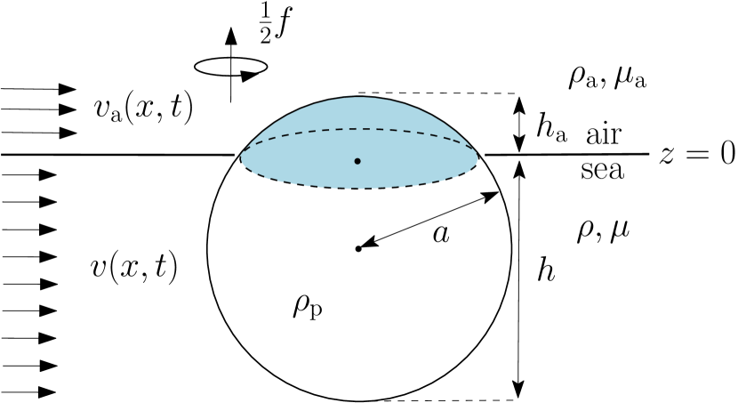
Figure 1: Solid spherical particle that floats at an assumed flat interface between homogeneous seawater and air, and is subjected to flow, added mass, and drag forces resulting from the action of unsteady, horizontally sheared ocean currents and winds. See text for variable and parameter definitions.

Let

$$\delta:=\frac{\rho}{\rho_{\mathrm{p}}},\quad\delta_{\mathrm{a}}:=\frac{\rho_{\mathrm{a}}}{\rho_{\mathrm{p}}}.$$ (1)

Clearly, $\delta\gg\delta_{\mathrm{a}}$. Let $0\leq\sigma\leq 1$ be the fraction of submerged (in seawater) particle volume. The emerged fraction then is $1-\sigma$, which is sometimes referred to as reserve buoyancy. Static (in the vertical) stability of the particle (Archimedes’ principle),

$$\sigma\delta+(1-\sigma)\delta_{\mathrm{a}}=1,$$ (2)

is satisfied for

$$\sigma=\frac{1-\delta_{\mathrm{a}}}{\delta-\delta_{\mathrm{a}}},$$ (3)

which requires

$$\delta\geq 1,\quad\delta_{\mathrm{a}}\leq 1.$$ (4)

We will conveniently assume Beron-Vera, Olascoaga, and Lumpkin (2016)

$$\delta_{\mathrm{a}}\ll 1,$$ (5)

so (3) can be well approximated by

$$\sigma=\delta^{-1}.$$ (6)

The height ($h_{\mathrm{a}}$) of the emerged spherical cap can be expressed in terms of $\delta$. This follows from equating its volume formula expressed in terms of $a$ and $h_{\mathrm{a}}$ with the volume of the emerged spherical cap. To wit,

$$\frac{\pi h_{\mathrm{a}}^{2}}{3}(3a-h_{\mathrm{a}})=(1-\delta^{-1})\frac{4}{3}\pi a^{3},$$ (7)

whose only physically meaningful root is

$$h_{\mathrm{a}}/a=\Phi:=\frac{\mathrm{i}\sqrt{3}}{2}\left(\frac{1}{\varphi}-\varphi\right)-\frac{1}{2\varphi}-\frac{\varphi}{2}+1$$ (8)

where

$$\varphi:=\sqrt[3]{\mathrm{i}\sqrt{1-(2\delta^{-1}-1)^{2}}+2\delta^{-1}-1}.$$ (9)

The depth ($h$) of the submerged spherical cap,

$$h=(2-\Phi)a.$$ (10)

For a neutrally buoyant particle, i.e., $\delta=1$, $\varphi=0$ and thus $\Phi=0$. Consequently, as expected, $h_{\mathrm{a}}=0$ (and hence $h=2a$). Near neutrality, $\Phi=\smash{\frac{2\sqrt{3}}{3}}\smash{\sqrt{\delta-1}}-\smash{\frac{2}{9}}(\delta-1)+O((\delta-1)^{2})$, which reveals the real nature of the root(s) of (7) explicitly. A half-emerged (equivalently, half-submerged) particle, namely, $h_{\mathrm{a}}=a=h$, corresponds to $\delta=2$. On the other hand, $h_{\mathrm{a}}\to 2a$ (and thus $h\to 0$) slowly as $\delta\to\infty$.

For future reference, the projected (in the flow direction) area of the emerged spherical cap, $A_{\mathrm{a}}$, can be readily seen to be given by

$$A_{\mathrm{a}}=\pi\Psi a^{2},\quad\Psi:=\pi^{-1}\cos^{-1}(1-\Phi)-\pi^{-1}(1-\Phi)\sqrt{1-(1-\Phi)^{2}},$$ (11)

a function of $\delta$ exclusively. In turn, the immersed projected area, denoted $A$, is equal to

$$A=\pi a^{2}-A_{\mathrm{a}}=\pi(1-\Psi)a^{2}.$$ (12)

When $\delta=1$, $A_{\mathrm{a}}=0$ (and hence $A=\pi a^{2}$), which immediately follows from $\Psi=\smash{\frac{16\sqrt[4]{3}}{9\pi}}(\delta-1)^{3/4}+O((\delta-1)^{5/4})$ as $\delta\to 1$. The situation in which $A_{\mathrm{a}}=\frac{1}{2}\pi a^{2}$ corresponds to $\delta=2$. Finally, $A_{\mathrm{a}}\to\pi a^{2}$ (and thus $A\to 0$) slowly as $\delta\to\infty$.

We close the setup with a few remarks. Ignoring the vertical shear of the ocean currents (resp., winds) below (resp., above) the interface over the extent of the particle piece that is immersed in the seawater (resp., air) is a reasonable approximation under the assumption that the particle is small. On the other hand, that the interface remains flat at all times is clearly a strong assumption. Recommendations for incorporating the effects of wind-induced (Stokes) drift are given below. In turn, ignoring lateral gradients and time variations of the carrying fluid density can be of consequence, particularly near frontal regions. Below we provide means for incorporating their effects as well.

III The Maxey–Riley set

III.1 The original fluid mechanics formulation

The exact motion of inertial particles such as that in Figure 1 is controlled by the Navier–Stokes equation with moving boundaries as such particles are extended objects in the fluid with their own boundaries. This approach results in complicated partial differential equations which are extremely difficult—if not impossible—to solve and analyze.

Here we are concerned with the approximation, formulated in terms of an ordinary differential equation, provided by the Maxey–Riley equation, which, as noted in the Introduction, has become the de-jure fluid mechanics paradigm for inertial particle dynamics.

More specifically, the Maxey–Riley equation is a classical mechanics Newton’s second law with several forcing terms that describe the motion of solid spherical particles immersed in the unsteady nonuniform flow of a homogeneous viscous fluid. Normalized by particle mass, $m_{\mathrm{p}}=\frac{4}{3}\pi a^{3}\rho_{\mathrm{p}}$, the relevant forcing terms for the horizontal motion of a sufficiently small particle are:

1. the flow force exerted on the particle by the undisturbed fluid,

   $$F_{\mathrm{flow}}=\frac{m_{\mathrm{f}}}{m_{\mathrm{p}}}\frac{\operatorname{D}\!{v_{\mathrm{f}}}}{\operatorname{D}\!{t}},$$ (13)

   where $m_{\mathrm{f}}=\frac{4}{3}\pi a^{3}\rho_{\mathrm{f}}$ is the mass of the displaced fluid (of density $\rho_{\mathrm{f}}$), and $\smash{\frac{\operatorname{D}\!{v_{\mathrm{f}}}}{\operatorname{D}\!{t}}}$ is the material derivative of the fluid velocity ($v_{\mathrm{f}}$) or its total derivative taken along the trajectory of a fluid particle, $x=X_{\mathrm{f}}(t)$, i.e., $\smash{\frac{\operatorname{D}\!{v_{\mathrm{f}}}}{\operatorname{D}\!{t}}}=\smash{\left[\frac{\operatorname{d}\!{}}{\operatorname{d}\!{t}}v_{\mathrm{f}}(x,t)\right]_{x=X_{\mathrm{f}}(t)}}=\partial_{t}v_{\mathrm{f}}+(\nabla v_{\mathrm{f}})v_{\mathrm{f}}$;

2. the added mass force resulting from part of the fluid moving with the particle,

   $$F_{\mathrm{mass}}=\frac{\frac{1}{2}m_{\mathrm{f}}}{m_{\mathrm{p}}}\left(\frac{\operatorname{D}\!{v_{\mathrm{f}}}}{\operatorname{D}\!{t}}-\dot{v}_{\mathrm{p}}\right),$$ (14)

   where $\dot{v}_{\mathrm{p}}$ is the acceleration of an inertial particle with trajectory $x=X_{\mathrm{p}}(t)$, i.e., $\dot{v}_{\mathrm{p}}=\smash{\frac{\operatorname{d}\!{}}{\operatorname{d}\!{t}}\left[v_{\mathrm{p}}(x,t)\right]_{x=X_{\mathrm{p}}(t)}}=\partial_{t}v_{\mathrm{p}}$ where $v_{\mathrm{p}}=\partial_{t}X_{\mathrm{p}}=\dot{x}$ is the inertial particle velocity;

3. the lift force, which arises when the particle rotates as it moves in a (horizontally) sheared flow,

   $$F_{\mathrm{lift}}=\frac{\frac{1}{2}m_{\mathrm{f}}}{m_{\mathrm{p}}}\omega_{\mathrm{f}}(v_{\mathrm{f}}-v_{\mathrm{p}})^{\perp},$$ (15)

   where $\omega_{\mathrm{f}}=\partial_{1}v^{2}_{\mathrm{f}}-\partial_{2}v^{1}_{\mathrm{f}}$ is the (vertical) vorticity of the fluid and

   $$w^{\perp}=Jw,\quad J:=\begin{pmatrix}0&-1\\ 1&0\end{pmatrix}$$ (16)

   for any vector $w$ in $\mathbb{R}^{2}$; and

4. the drag force caused by the fluid viscosity,

   $$F_{\mathrm{drag}}=\frac{12\mu_{\mathrm{f}}\frac{A_{\mathrm{f}}}{\ell_{\mathrm{f}}}}{m_{\mathrm{p}}}(v_{\mathrm{f}}-v_{\mathrm{p}}),$$ (17)

   where $\mu_{\mathrm{f}}$ is the dynamic viscosity of the fluid, and $A_{\mathrm{f}}$ ($=\pi a^{2}$) is the projected area of the particle and $\ell_{\mathrm{f}}$ ($=2a$) is the characteristic projected length, which we have intentionally left unspecified for future appropriate evaluation.

Except for the lift force (15), due to Auton (1987), the above forces are included in the original formulation by Maxey and Riley (1983) (cf. also Gatignol (1983)), yet with a form of the added mass term different than (14), which corresponds to the correction due to Auton, Hunt, and Prud’homme (1988). A Maxey–Riley model with lift force, which has not been so far considered in ocean dynamics despite its relevance in the presence of unbalanced (submesoscale) motions (e.g., Beron-Vera et al. (2018)), can be found in Montabone (2002, Chapter 4) (cf. similar forms in Henderson, Gwynllyw, and Barenghi (2007); Sapsis et al. (2011)).

In writing (14) and (17), terms proportional to $\nabla^{2}v_{\mathrm{f}}$, so-called Faxen corrections, have been ignored. These account for the horizontal variation of the flow field across the particle, which is negligible for a particle with a radius much smaller than the typical length scale of the flow. Also, the complete set of Maxey–Riley forces involves an additional term, the Basset–Boussinesq history or memory term. This is an integral term that accounts for the lagging boundary layer developed around the particle. The memory term turns the Maxey–Riley set into a fractional differential equation that does not generate a dynamical system as the corresponding flow map does not satisfy a semi-group property Farazmand and Haller (2015); Langlois, Farazmand, and Haller (2015). Numerical experimentation Daitche and Tél (2011) reveals that the Basset history term mainly tends to slow down the inertial particle motion. More rigorously, Langlois, Farazmand, and Haller (2015) show that the particle velocity decays algebraically, rather than exponentially as in the absence of the memory term, in time to a limit that is close, in the square of the particle’s radius, to the carrying fluid velocity. The memory term cannot be neglected on sufficiently small particle assumption grounds Daitche and Tél (2014); Langlois, Farazmand, and Haller (2015), but it may be under the assumption that the time it takes a particle to return to a region that has visited earlier is long compared to the time scale of the flow Sudharsan, Brunton, and Riley (2016), condition that should not be too difficult to be satisfied in the ocean, except, for instance, inside vortices.

III.2 The proposed adaptation to surface ocean dynamics

We first account for the geophysical nature of the fluid by including the Coriolis force. This amounts to replacing (13) and (14) with

$$F_{\mathrm{flow}}=\frac{m_{\mathrm{f}}}{m_{\mathrm{p}}}\left(\frac{\operatorname{D}\!{v_{\mathrm{f}}}}{\operatorname{D}\!{t}}+fv_{\mathrm{f}}^{\bot}\right)$$ (18)

and

$$F_{\mathrm{mass}}=\frac{\frac{1}{2}m_{\mathrm{f}}}{m_{\mathrm{p}}}\left(\frac{\operatorname{D}\!{v_{\mathrm{f}}}}{\operatorname{D}\!{t}}+fv_{\mathrm{f}}^{\bot}-\dot{v}_{\mathrm{p}}-fv_{\mathrm{p}}^{\bot}\right),$$ (19)

respectively. Geometric terms due to the planet’s sphericity, which should be included when $f$ is allowed to vary with $x^{2}$, making $(x^{1},x^{2})$ curvilinear rather than Cartesian Pedlosky (1987), were omitted as traditionally done for simplicity, yet recognizing that some consequences may be expected Ripa (1997a). Nevertheless, the full spherical form of the equations derived below, appropriate for operational use, is given in Appendix A.

Then, noting that fluid variables and parameters take different values when pertaining to seawater or air, e.g.,

$$v_{\mathrm{f}}(x,z,t)=\begin{cases}v_{\mathrm{a}}(x,t)&\text{if }z\in(0,h_{\mathrm{a}}],\\ v(x,t)&\text{if }z\in[-h,0),\end{cases}$$ (20)

we write

$$\dot{v}_{\mathrm{p}}+fv_{\mathrm{p}}^{\perp}=\langle F_{\mathrm{flow}}\rangle+\langle F_{\mathrm{mass}}\rangle+\langle F_{\mathrm{lift}}\rangle+\langle F_{\mathrm{drag}}\rangle,$$ (21)

where $\langle\,\rangle$ is an average over $z\in[-h,h_{\mathrm{a}}]$.

Specifically,

$$\langle F_{\mathrm{flow}}\rangle={} \frac{1}{2a}\int_{-h}^{h_{\mathrm{a}}}\frac{m_{\mathrm{f}}}{m_{\mathrm{p}}}\left(\frac{\operatorname{D}\!{v_{\mathrm{f}}}}{\operatorname{D}\!{t}}+fv_{\mathrm{f}}^{\bot}\right)\operatorname{d}\!{z}$$

$$={} \frac{1}{2a}\int_{(\Phi-2)a}^{0}\frac{\delta^{-1}\frac{4}{3}\pi a^{3}\rho}{\frac{4}{3}\pi a^{3}\rho_{\mathrm{p}}}\left(\frac{\operatorname{D}\!{v}}{\operatorname{D}\!{t}}+fv^{\bot}\right)\operatorname{d}\!{z}$$

$$+\frac{1}{2a}\int_{0}^{\Phi a}\frac{(1-\delta^{-1})\frac{4}{3}\pi a^{3}\rho_{\mathrm{a}}}{\frac{4}{3}\pi a^{3}\rho_{\mathrm{p}}}\left(\frac{\operatorname{D}\!{v_{\mathrm{a}}}}{\operatorname{D}\!{t}}+fv_{\mathrm{a}}^{\bot}\right)\operatorname{d}\!{z}$$

$$\overset{\hphantom{\delta_{\mathrm{a}}\ll 1}}{=}{} \frac{1}{2}(2-\Phi)\left(\frac{\operatorname{D}\!{v}}{\operatorname{D}\!{t}}+fv^{\bot}\right)+\frac{1}{2}(1-\delta^{-1})\Phi\delta_{\mathrm{a}}\left(\frac{\operatorname{D}\!{v_{\mathrm{a}}}}{\operatorname{D}\!{t}}+fv_{\mathrm{a}}^{\bot}\right),$$ (22)

where $\smash{\frac{\operatorname{D}\!{}}{\operatorname{D}\!{t}}}v$ (resp., $\smash{\frac{\operatorname{D}\!{}}{\operatorname{D}\!{t}}}v_{\mathrm{a}}$) is understood to be taken along the trajectory of a seawater (resp., air) particle, obtained by solving $\dot{x}=v$ (resp., $\dot{x}=v_{\mathrm{a}}$), namely, $\smash{\frac{\operatorname{D}\!{}}{\operatorname{D}\!{t}}}v=\partial_{t}v+(\nabla v)v$ (resp., $\smash{\frac{\operatorname{D}\!{}}{\operatorname{D}\!{t}}}v_{\mathrm{a}}=\partial_{t}v_{\mathrm{a}}+(\nabla v_{\mathrm{a}})v_{\mathrm{a}}$). Taking into account that $\delta_{\mathrm{a}}\ll 1$, (22) is well approximated by

$$\langle F_{\mathrm{flow}}\rangle=\left(1-\frac{\Phi}{2}\right)\left(\frac{\operatorname{D}\!{v}}{\operatorname{D}\!{t}}+fv^{\bot}\right).$$ (23)

Similarly,

$$\langle F_{\mathrm{mass}}\rangle \overset{\hphantom{\delta_{\mathrm{a}}\ll 1}}{=}\frac{1}{2a}\int_{-h}^{h_{\mathrm{a}}}\frac{\frac{1}{2}m_{\mathrm{f}}}{m_{\mathrm{p}}}\left(\frac{\operatorname{D}\!{v_{\mathrm{f}}}}{\operatorname{D}\!{t}}+fv_{\mathrm{f}}^{\bot}-\dot{v}_{\mathrm{p}}-fv_{\mathrm{p}}^{\bot}\right)\operatorname{d}\!{z}$$

$$\overset{\delta_{\mathrm{a}}\ll 1}{=}\frac{1}{2}\left(1-\frac{\Phi}{2}\right)\left(\frac{\operatorname{D}\!{v}}{\operatorname{D}\!{t}}+fv^{\bot}-\dot{v}_{\mathrm{p}}-fv_{\mathrm{p}}^{\bot}\right)$$ (24)

and

$$\langle F_{\mathrm{lift}}\rangle \overset{\hphantom{\delta_{\mathrm{a}}\ll 1}}{=}\frac{1}{2a}\int_{-h}^{h_{\mathrm{a}}}\frac{\frac{1}{2}m_{\mathrm{f}}}{m_{\mathrm{p}}}\omega_{\mathrm{f}}\left(v_{\mathrm{f}}-v_{\mathrm{p}}\right)^{\perp}\operatorname{d}\!{z}$$

$$\overset{\delta_{\mathrm{a}}\ll 1}{=}\frac{1}{2}\left(1-\frac{\Phi}{2}\right)\omega\left(v-v_{\mathrm{p}}\right)^{\perp}.$$ (25)

Now, to evaluate the drag force, appropriate projected length scales for the submerged and emerged particle pieces must be chosen. We conveniently take $\ell=kh$ and $\ell_{\mathrm{a}}=k_{\mathrm{a}}h_{\mathrm{a}}$ for some $k,k_{\mathrm{a}}>0$. For instance, if $\delta=1$ (resp., $\delta\to\infty$), namely, the particle is completely submerged below (resp., emerged above) the sea surface, $k=1$ (resp., $k_{\mathrm{a}}=1$) is an appropriate choice so $\ell=2a$ (resp., $\ell_{\mathrm{a}}=2a$). Thus, with this in mind,

$$\langle F_{\mathrm{drag}}\rangle= {}\frac{1}{2a}\int_{-h}^{h_{\mathrm{a}}}\frac{12\mu_{\mathrm{f}}\frac{A_{\mathrm{f}}}{\ell_{\mathrm{f}}}}{m_{\mathrm{p}}}(v_{\mathrm{f}}-v_{\mathrm{p}})\operatorname{d}\!{z}$$

$$= {}\frac{1}{2a}\int_{(\Phi-2)a}^{0}\frac{12\mu\frac{\pi(1-\Psi)a^{2}}{k(2-\Phi)a}}{\frac{4}{3}\pi a^{3}\rho_{\mathrm{p}}}(v-v_{\mathrm{p}})\operatorname{d}\!{z}$$

$$+\frac{1}{2a}\int_{0}^{\Phi a}\frac{12\mu_{\mathrm{a}}\frac{\pi\Psi a^{2}}{k_{\mathrm{a}}\Phi a}}{\frac{4}{3}\pi a^{3}\rho_{\mathrm{p}}}(v_{\mathrm{a}}-v_{\mathrm{p}})\operatorname{d}\!{z}$$

$$= {}\frac{9\mu k^{-1}(1-\Psi)}{2\rho_{\mathrm{p}}a^{2}}(v-v_{\mathrm{p}})+\frac{9\mu_{\mathrm{a}}k_{\mathrm{a}}^{-1}\Psi}{2\rho_{\mathrm{p}}a^{2}}(v_{\mathrm{a}}-v_{\mathrm{p}})$$

$$= {}\frac{3}{2}\left(1-\frac{\Phi}{6}\right)\frac{u-v_{\mathrm{p}}}{\tau},$$ (26)

where

$$u:=(1-\alpha)v+\alpha v_{\mathrm{a}},$$ (27)

and the parameters

$$\tau:=\frac{1-\frac{1}{6}\Phi}{3\left(k^{-1}(1-\Psi)+\gamma k_{\mathrm{a}}^{-1}\Psi\right)\delta}\cdot\frac{a^{2}}{\mu/\rho},\quad\alpha:=\frac{\gamma k_{\mathrm{a}}^{-1}\Psi}{k^{-1}(1-\Psi)+\gamma k_{\mathrm{a}}^{-1}\Psi},\quad\gamma:=\frac{\mu_{\mathrm{a}}}{\mu}.$$ (28)

Finally, plugging (23)–(26) in (21), we obtain, after some algebraic manipulation,

$$\boxed{\dot{v}_{\mathrm{p}}+\left(f+\tfrac{1}{3}R\omega\right)v_{\mathrm{p}}^{\perp}+\tau^{-1}v_{\mathrm{p}}=R\frac{\operatorname{D}\!{v}}{\operatorname{D}\!{t}}+R\left(f+\tfrac{1}{3}\omega\right)v^{\perp}+\tau^{-1}u,}$$ (29)

where

$$\quad R:=\frac{1-\frac{1}{2}\Phi}{1-\frac{1}{6}\Phi},$$ (30)

which is the explicit form of the Maxey–Riley set proposed in this paper. As a second-order ordinary differential equation in position, to integrate this classical mechanics motion law, not only initial position has to be specified but clearly also initial velocity.

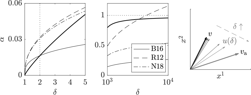
Figure 2: (left and middle) The behavior of the leeway factor $\alpha$ in (28) as a function of $\delta$ (with $\gamma=1/60$ and $k=1=k_{\mathrm{a}}$). B16, R12, and N18 indicate $\alpha(\delta)$ curves derived by Beron-Vera, Olascoaga, and Lumpkin (2016), Röhrs et al. (2012), and Nesterov (2018), respectively. (right) The $\delta$-weighted velocity in (27) for selected values of $\delta$.

In (28) parameter $\gamma>0$ is less than unity ($\gamma\approx 1/60$, typically), while parameters $\alpha$ and $\tau$ behave as follows. First recall that $0\leq\Phi<2$, so $0\leq\Psi<1$. Then given that $k,k_{\mathrm{a}}>0$, it is easy to see that $0\leq\alpha<1$. More specifically, $\alpha=0$ when $\delta=1$ and $\alpha\to 1$ slowly as $\delta\to\infty$ (cf. thick curve(s) in the left and middle panels of Figure 2). Parameter $\tau$, with units of time and representing a generalization of the so-called Stokes time Sozza et al. (2016), decays as a function of $\delta$ from $\smash{\frac{a^{2}}{3\mu/\rho}}$ (since $k=1$ is an appropriate choice when $\delta=1$) to 0. Yet it can be brought arbitrarily close to 0 for finite $\delta$ if the inertial particle radius ($a$) is small enough. Finally, parameter $R$ in (30) decays from 1 to 0 as $\delta$ increases from 1.

Because $\alpha\geq 0$, the convex combination $u$ in (27) can be interpreted as a $\delta$-weighted average of the seawater ($v$) and air ($v_{\mathrm{a}}$) velocities. In fact, $u$ coincides with $v$ in the neutrally buoyant case ($\delta=1$) in which the particle lies fully immersed in the seawater below the surface, whereas $u$ approaches $v_{\mathrm{a}}$ as the particle lightens (i.e., as $\delta$ departs from unity) until it becomes fully exposed to the air above the sea surface.

The original Maxey–Riley set was derived under the assumption that particle Reynolds number is less than unity, so the Stokes law for drag (17) can be used. The particle Reynolds number, $\mathrm{Re_{p}}:=\smash{\frac{V_{\mathrm{slip}}\ell_{\mathrm{f}}}{\mu_{\mathrm{f}}/\rho_{\mathrm{f}}}}$ where $V_{\mathrm{slip}}$ is a measure of the magnitude of the slip velocity, i.e., that of the particle velocity ($v_{\mathrm{p}}$) relative to that of the carrying flow ($v_{\mathrm{f}}$). The asymptotic analysis of set (29) as $\tau\to 0$ (or, equivalently, $a\to 0$ if $\delta$ is kept finite) in the following section will reveal that an appropriate measure of $V_{\mathrm{slip}}$ is that of $|v_{\mathrm{p}}-u|$. Furthermore, this asymptotic analysis will reveal that $v_{\mathrm{p}}-u=O(\tau)$, so the use of the Stokes drag law will be well justified for sufficiently small particles independent of the magnitude of the carrying flow velocity, effectively given by that of the $\delta$-weighted velocity $u$, and the carrying fluid kinematic viscosity, taken as that of either the seawater or the air, or some average thereof.

As it follows from the aforementioned asymptotic analysis, in the sizeless particle case ($\tau=0$), $v_{\mathrm{p}}$ coincides with $u$. The search-and-rescue literature (e.g., Breivik and Allen Breivik and Allen (2008) and references therein) often models windage effects on the drift of objects as an additive contribution to the ocean current. In our notation this is $v_{\mathrm{p}}=u$ for some $\alpha$, commonly referred to as a leeway factor. Obtained empirically, $\alpha$ is taken as some fixed value in the range 1–5% Duhec et al. (2015); Trinanes et al. (2016); Allshouse et al. (2017). However, formulas depending on the projected areas of emerged and submerged pieces of the objects and their floatation characteristics have been proposed Röhrs et al. (2012); Nesterov (2018). These formulas, seemingly valid for arbitrary shaped objects, are obtained by assuming that the drag in the seawater is exactly balanced by that in the air above, a hard to justify assumption apparently first made by Geyer (1989). Furthermore, these formulas consider a quadratic (in the slip particle) drag law. Such a law assumes that the particle is in Newton’s (rather than Stokes’) regime, which is valid for high particle Reynolds numbers Kundu, Cohen, and Dowling (2012). Assuming that the (constant) drag coefficient is the same below and above the sea surface as in Nesterov (2018), we show in the left and right panels of Figure 2 the resulting leeway factors as a function of $\delta$ for the case of spherical objects. Note for instance that the formula derived by Röhrs et al. (2012) (cf. also Daniel et al. (2002)) exceeds unity in the $\delta\to\infty$ limit, while that of Nesterov (2018) has not converged to unity for $\delta$ values for which a particle is almost completely exposed to the air (indeed, for $\delta=10^{3}$, $\Phi=h_{\mathrm{a}}/2a=0.9816$). For smaller $\delta$ values the leeway factors derived by these authors exceed $\alpha$ in (28) for $k=1=k_{\mathrm{a}}$. Figure 2 also shows the $\alpha$ curve obtained by Beron-Vera et al. (2015). Note that it lies below that one derived here, and it also very slowly tends to unity as $\delta\to\infty$. Because of this and the additional freedom in choosing $k$ and $k_{\mathrm{a}}$, the new formula for $u$ has more margin (leeway!) than its predecessor for modeling in an wider range of conditions.

III.3 Limitations and heuristic extensions

The Maxey–Riley theory for inertial ocean dynamics proposed in this paper has several limitations. First is its restriction to spherical particles (objects), which constrains its ability to account for the motion of flotsam in general. Posing the general problem of a rigid body of arbitrary shape moving in the flow of a fluid is a very difficult task, which is beyond the scope of our paper. However, a simple heuristic fix, which can be expected to be valid for sufficiently small objects, is to multiply $\tau$ in (28) by $K$, a shape factor satisfying Ganser (1993)

$$K^{-1}=\frac{1}{3}\frac{a_{\mathrm{n}}}{a_{\mathrm{v}}}+\frac{2}{3}\frac{a_{\mathrm{s}}}{a_{\mathrm{v}}}.$$ (31)

Here $a_{\mathrm{n}}$, $a_{\mathrm{s}}$, and $a_{\mathrm{v}}$ are the radii of the sphere with equivalent projected area, surface area, and equivalent volume, respectively, whose average provide an appropriate choice for $a$. A caveat is that $K$ is nonunique for nonisometric shapes owing to orientation dependence. If the orientation is not known, Ganser (1993) recommends to use the average of the two extreme values of $K$.

Second, in deriving the Maxey–Riley set (29) we have assumed a flat air–sea interface, ignoring the effects of the Stokes drift arising from material orbits not being closed under a wavy water surface Phillips (1997). A first step toward including these effects is at the level of the ocean component of the carrying flow, $v$. One option is to take $v$ as the output from a coupled ocean–wave circulation model Breivik et al. (2015). Another, less challenging option is to add Craik (1982) to any given representation of $v$ that ignores gravity wave effects, a Stokes drift velocity $v_{\mathrm{S}}$. To estimate $v_{\mathrm{S}}$ there several options depending on whether the directional wave spectrum is known Jenkins (1989) or not Webb and Fox-Kemper (2011); Tamura, Miyazawa, and Oey (2012); Breivik, Bidlot, and Janssen (2016). The simplest rule is to make $v_{\mathrm{S}}$ a small fraction of the air velocity $v_{\mathrm{a}}$ assuming that wind and waves are aligned and that the wave field is in a steady state Wu (1983).

Finally, ignoring lateral gradients and temporal variations of the density of the advecting fluid can be consequential, particularly near frontal regions. While the original Maxey–Riley set was derived for the case of homogeneous carrying fluid density, heuristic extensions to the inhomogeneous case have been proposed Tanga and Provenzale (1994), which can be considered. More specifically, Tanga and Provenzale (1994) considered the motion of particles in a stable stratified fluid with buoyancy oscillating around a reference density. This translated into making parameter $\delta$ in the original Maxey–Riley set a periodic function of time by making $\rho_{\mathrm{p}}$ a periodic function of time while $\rho$ is kept constant. These heuristics may be modified to investigate the situation in which an inertial particle with fixed density $\rho_{\mathrm{p}}$ moves through an ambient fluid with density $\rho$ changing in space and time. This corresponds to making $\delta$ a predefined arbitrary function of $x$ and $t$. In our case, $\rho$ is the density of the seawater. The air density does not appear in the Maxey–Riley set (29). Indeed, the only air parameter is the air viscosity, which can be kept safely fixed. The condition $\delta(x,t)\geq 1$ needed for the Maxey–Riley set to remain valid should not be difficult to be satisfied for an initially sufficiently buoyant particle.

IV Behavior at limiting particle buoyancies and small-size asymptotics

IV.1 The neutrally buoyant case

Setting $\delta=1$, the Maxey–Riley set (29) reduces to

$$\dot{v}_{\mathrm{p}}+\left(f+\tfrac{1}{3}\omega\right)v_{\mathrm{p}}^{\perp}+\tau^{-1}v_{\mathrm{p}}=\frac{\operatorname{D}\!{v}}{\operatorname{D}\!{t}}+\left(f+\tfrac{1}{3}\omega\right)v^{\perp}+\tau^{-1}v,$$ (32)

with

$$\tau=\frac{a^{2}}{3\mu/\rho}.$$ (33)

The resulting set coincides exactly with the Maxey–Riley equation for neutrally buoyant particles as considered in Montabone (2002, Chapter 7), which is the standard Maxey–Riley with Coriolis and lift forces included, but with Faxen corrections and memory term neglected (cf. Cartwright et al. (2010), Section 4.1) Evaluated at $\delta=1$, the Maxey–Riley set for inertial surface ocean dynamics derived by Beron-Vera, Olascoaga, and Lumpkin (2016) has the same form as (32) except for the terms produced by the lift force, which was not included in that formulation.

Such dynamics are quite special: they coincide, irrespective of the size of the particle (equivalently, the value of $\tau$), with those of Lagrangian (seawater in the present case) particles if $v_{\mathrm{p}}=v$ initially. To see this, following Babiano et al. (2000) closely, we add and subtract $(\nabla v)v_{\mathrm{p}}$ to and from the right-hand-side of (32) so it recasts as the linear system

$$\dot{y}=Ay,\quad y:=v_{\mathrm{p}}-v,\quad A:=-\left(\nabla v+\left(f+\tfrac{1}{3}\omega\right)J+\tau^{-1}\operatorname{Id}\right),$$ (34)

where $\dot{v}=\smash{\frac{\operatorname{d}\!{}}{\operatorname{d}\!{t}}}v=\partial_{t}v+(\nabla v)v_{\mathrm{p}}$ is the total derivative of $v$ taken a long a particle trajectory, satisfying $\dot{x}=v_{\mathrm{p}}$. Clearly, the trivial solution $y=0$ is invariant under the dynamics. In other words,

$$\mathcal{N}:=\{(x,t,v_{\mathrm{p}})\mid v_{\mathrm{p}}=v(x,t),\ (x,t)\in D\times I\}$$ (35)

represents an invariant manifold (modulo its boundary, which has corners due to finiteness of $I$) that is unique as it does not depend on the choice of $\tau$.

However, in the nonrotating case ($f=0$) and ignoring the lift force, the motion of neutrally buoyant particles of finite size is known from numerical analysis Babiano et al. (2000); Vilela, de Moura, and Grebogi (2006) as well as laboratory experimentation Sapsis et al. (2011) to possibly deviate from that of Lagrangian particles. Sapsis and Haller (2008) rigorously addressed this problem by deriving a sufficient condition for global attractivity of $\mathcal{N}$ in that case as well as a necessary condition for local instability of $\mathcal{N}$. It turns out that, because $J=-J^{\top}$, the same conditions as those obtained by Sapsis and Haller (2008) are found in the present geophysical setting with Coriolis and lift forces (cf. Appendix B for details). In other words, these terms contribute to neither setting the attractivity property of $\mathcal{N}$, nor controlling the growth of perturbations off $\mathcal{N}$.

Specifically, let $S:=\smash{\frac{1}{2}}(\nabla v+(\nabla v)^{\top})$ be the rate-of-strain tensor. Then for $\mathcal{N}$ to be globally attracting, i.e., for $v_{\mathrm{p}}$ to approach $v$ and hence neutrally buoyant finite-size particle motion to synchronize with seawater particle motion in the long run in $D$, it is sufficient that $S+\tau^{-1}\operatorname{Id}$ be positive definite for all $x\in D$ over the time interval $I$, or, equivalently,

$$\tau<\frac{2}{\sqrt{S_{\mathrm{n}}^{2}+S_{\mathrm{s}}^{2}}-\nabla\cdot v},$$ (36)

where $S_{\mathrm{n}}:=\partial_{1}v^{1}-\partial_{2}v^{2}$ and $S_{\mathrm{s}}:=\partial_{2}v^{1}+\partial_{1}v^{2}$ respectively are normal and shear strain components, for all $x\in D$ over the time interval $I$. Clearly, for the latter to be realized over the finite-time interval $I$, $v_{\mathrm{p}}$ must initially lie sufficiently close to $v$, a restriction that is not required when $I=\mathbb{R}$ as in Sapsis and Haller (2008). In the geophysically relevant incompressible case, (36) reduces to $\tau<\smash{1/\sqrt{|\det S|}}$ for all $(x,t)\in D\times I$. On the other hand, instantaneous divergence away from $\mathcal{N}$ will take place where $S+\tau^{-1}\operatorname{Id}$ is sign indefinite, or, equivalently, where (36) is violated.

IV.2 The maximally buoyant case

The limit $\delta\to\infty$ is dynamically less sophisticated than the $\delta=1$ case of the previous section. In this limit, $\tau=0$ and hence the Maxey–Riley set (29) reduces to simply

$$v_{\mathrm{p}}=v_{\mathrm{a}}.$$ (37)

A maximally buoyant particle lies on the assumed flat surface ocean and, irrespective of its size, its motion is synchronized at all times with that of air particle (i.e., Lagrangian) motion. In this limit, (29) and the Maxey–Riley set derived by Beron-Vera, Olascoaga, and Lumpkin (2016) behave identically.

IV.3 Slow manifold reduction

Because of the small particle size assumption, it is natural to investigate the asymptotic behavior of the Maxey–Riley set (29) as $\tau\to 0$, as it has been done for the Maxey–Riley set in its standard fluid mechanics form Rubin, Jones, and Maxey (1995); Burns, Davis, and Moore (1999); Mograbi and Bar-Ziv (2006); Haller and Sapsis (2008) and its earlier adaptations for ocean dynamics Beron-Vera et al. (2015); Beron-Vera, Olascoaga, and Lumpkin (2016).

To carry the above investigation formally, we first rescale space and time by a characteristic length scale $L$ and characteristic time scale $T=L/V$ where $V$ is a characteristic velocity. Then write the Maxey–Riley set (29) as an autonomous dynamical system in the extended phase space $D\times I\times\mathbb{R}^{2}$ with variables $(x,\varphi,v_{\mathrm{p}})$, where $\varphi=t$, namely,

$$\dot{x} =v_{\mathrm{p}},$$ (38)

$$\dot{\varphi} =1,$$ (39)

$$\tau\dot{v}_{\mathrm{p}} =u-v_{\mathrm{p}}-\tau\left(f+\tfrac{1}{3}R\omega\right)v_{\mathrm{p}}^{\perp}+\tau R\frac{\operatorname{D}\!{v}}{\operatorname{D}\!{t}}+\tau R\left(f+\tfrac{1}{3}\omega\right)v^{\perp}.$$ (40)

All variables are here understood with no fear of confusion to be dimensionless. In particular, the dimensionless $\tau$ parameter,

$$\tau=\frac{(1-\frac{1}{6}\Phi)}{3\left(k^{-1}(1-\Psi)+\gamma k_{\mathrm{a}}^{-1}\Psi\right)\delta}\cdot\mathrm{St},$$ (41)

where $\mathrm{St}:=\smash{\left(\frac{a}{L}\right)^{2}}\mathrm{Re}$ is a Stokes number with $\mathrm{Re}:=\smash{\frac{VL}{\mu/\rho}}$ the Reynolds number. We assume

$$\tau\ll 1.$$ (42)

Now, from (38)–(39) it is clear that $v_{\mathrm{p}}$ is a fast variable changing at $O(\tau^{-1})$ speed while $(x,\varphi)$, changing at $O(1)$ speed, is a slow variable. The coexistence of fast and slow variables in system (38)–(39) makes it a singular perturbation problem Fenichel (1979); Jones (1995). To see this, we rewrite (38)–(39) using the fast timescale Haller and Sapsis (2008)

$$\mathcal{T}:=\frac{t-t_{0}}{\tau},$$ (43)

where $t_{0}\neq 0$, namely,

$$x^{\prime} =\tau v_{\mathrm{p}},$$ (44)

$$\varphi^{\prime} =\tau,$$ (45)

$$v_{\mathrm{p}}^{\prime} =u-v_{\mathrm{p}}-\tau\left(f+\tfrac{1}{3}R\omega\right)v_{\mathrm{p}}^{\perp}+\tau R\frac{\operatorname{D}\!{v}}{\operatorname{D}\!{t}}+\tau R\left(f+\tfrac{1}{3}\omega\right)v^{\perp},$$ (46)

where ${}^{\prime}:=\smash{\frac{\operatorname{d}\!{}}{\operatorname{d}\!{\mathcal{T}}}}$. The $\tau=0$ limit of (44)–(46) has an invariant normally hyperbolic manifold (modulo its boundary) $\mathcal{S}_{0}$ filled with fixed points, which globally attracts its solutions exponentially fast in time. This critical manifold has a graph representation:

$$\mathcal{S}_{0}=\{(x,\varphi,v_{\mathrm{p}})\mid v_{\mathrm{p}}=u(x,\varphi),\ x\in D,\,\varphi\in I\}.$$ (47)

The motion of (44)–(46) at $\tau=0$ is trivial: trajectories off $\mathcal{S}_{0}$ are attracted to it and get stuck there. By contrast, (38)–(40) at $\tau=0$ blows the motion on $\mathcal{S}_{0}$ to produce nontrivial behavior on it, whereas the motion off $\mathcal{S}_{0}$ is not defined. The idea of Fenichel’s Fenichel (1979); Jones (1995) geometric singular perturbation theory is to enable realization of the fast and slow aspects of the motion simultaneously as follows.

Assume that $v$ and $v_{\mathrm{a}}$, and hence their $\delta$-weighted average $u$, are $C^{r}$ smooth (i.e., $r$ times continuously differentiable) in their arguments with $r>1$. Then when $0<\tau\ll 1$, there exists a unique (up to an $O(\smash{\mathrm{e}^{-1/\tau}})$ error), locally invariant (i.e., with trajectories only possibly leaving through the boundary), globally attracting manifold

$$\mathcal{S}_{\tau}:=\left\{(x,\varphi,v_{\mathrm{p}})\mid v_{\mathrm{p}}=u_{\tau}(x,\varphi),\ (x,\varphi)\in D\times I\right\},$$ (48)

where

$$u_{\tau}(x,\varphi)=u(x,\varphi)+\sum\nolimits_{1}^{r}\tau^{n}u_{n}(x,\varphi)+O(\tau^{r+1}),$$ (49)

which is $C^{r}$ $O(\tau)$-close to $\mathcal{S}_{0}$ and $C^{r}$-diffeomorphic to it. The manifold $\mathcal{S}_{\tau}$ is called a slow manifold since the restriction of (38)–(40) to $\mathcal{S}_{\tau}$ is a slowly varying system, namely,

$$x^{\prime}=\tau\left.v_{\mathrm{p}}\right|_{\mathcal{S}_{\tau}}=\tau u(x,t)+\sum\nolimits_{1}^{r}\tau^{n+1}u_{n}(x,t)+O(\tau^{r+2}).$$ (50)

Moreover, this system controls the motion off $\mathcal{S}_{\tau}$ as follows. When $\tau=0$, each point off $\mathcal{S}_{0}$ belongs to the stable manifold of $\mathcal{S}_{0}$, which is foliated by its distinct stable fibers (stable manifolds of points on $\mathcal{S}_{0}$). The stable manifold of $\mathcal{S}_{0}$ and its stable fibers perturb along with $\mathcal{S}_{0}$. Consequently, for $0<\tau\ll 1$ each point off $\mathcal{S}_{\tau}$ is connected to a point on $\mathcal{S}_{\tau}$ by a fiber in the sense that it follows a trajectory that approaches its partner on $\mathcal{S}_{\tau}$ exponentially fast in time.

The function defining $\mathcal{S}_{\tau}$ is found by plugging the Taylor expansion in (49) into (44)–(46) and equating $\tau$-power terms. This gives, following steps similar to those in Appendix C,

$$u_{1}={} R\frac{\operatorname{D}\!{v}}{\operatorname{D}\!{t}}+R\left(f+\tfrac{1}{3}\omega\right)v^{\perp}-\frac{\operatorname{D}\!{u}}{\operatorname{D}\!{t}}-\left(f+\tfrac{1}{3}R\omega\right)u^{\perp}$$ (51)

$$u_{n}={} -\left(f+\tfrac{1}{3}R\omega\right)u_{n-1}^{\perp}$$

$$-\partial_{t}u_{n-1}-(\nabla u_{n-1})u-(\nabla u)u_{n-1}$$

$$-\sum\nolimits_{m=1}^{n-2}(\nabla u_{m})u_{n-m-1},\quad n\geq 2,$$ (52)

which fully determine $\mathcal{S}_{\tau}$. Switching back to the original time scale, the leading-order contribution to the Maxey–Riley system (29) on the slow manifold $\mathcal{S}_{\tau}$, in dimensional variables, is

$$\boxed{\dot{x}=v_{\mathrm{p}}\sim u+\tau\bigg{(}R\frac{\operatorname{D}\!{v}}{\operatorname{D}\!{t}}+R\left(f+\tfrac{1}{3}\omega\right)v^{\perp}-\frac{\operatorname{D}\!{u}}{\operatorname{D}\!{t}}-\left(f+\tfrac{1}{3}R\omega\right)u^{\perp}\bigg{)}}$$ (53)

as $\tau\to 0$. The reduced system (53) may be referred to as the inertial equation following nomenclature employed in earlier work Haller and Sapsis (2008); Beron-Vera et al. (2015).

Several remarks are in order. Firstly, the nondimensionalization above makes sense in the $\delta$-range where $\alpha$ is small, which is rather large (cf. Fig. 2). Indeed, since the magnitude of $v$ is typically smaller than that of $v_{\mathrm{a}}$, if $v$ is scaled using $V$, then $v_{\mathrm{a}}$ can be scaled using $\alpha^{-1}V$ under the assumption that $\alpha$ is small enough. This way $u$ will scale like $V$ as required.

Second, rapid changes in time of the carrying flow velocity, represented by $u$, will lead to rapid changes on $\mathcal{S}_{\tau}$, thereby hindering its efficacy in absorbing trajectories of the Maxey–Riley equation over finite time Haller and Sapsis (2008, 2010). Yet appropriate redefinition of the slow manifold involving history integrals of the fast time scale Roberts (2008) can compensate the effects of such rapid variations even if they are stochastic.

Third, unlike the Maxey–Riley set (29), its slow manifold reduction (53) does not require specification of the initial velocity, which is not known in general. Also, (53) does not include the term $v_{\mathrm{p}}/\tau$ present in (29). This term is known to produce numerical instability in long backward-time integration, e.g., as required is source inversion Olascoaga et al. (2016); Miron et al. (2019a), unless specialized numerical techniques Gear and Kevrekidis (2003) are used. Furthermore, according to Theorem 2 of Sapsis and Haller (2008), the starting position $x(t_{0})$ of any solution $(x(t),v_{\mathrm{p}}(t))$ of (53) may be recovered with $O(\tau)$ precision.

Fourth, representing a simpler model than the full Maxey–Riley set (29), the reduced equation (53) can provide insight that is difficult—if not impossible—to be gained from the analysis of the full system, as we show below.

Lastly, we note one difference with the slow manifold of the Maxey–Riley set in its standard fluid mechanics setting with lift force. As we show in Appendix C, the lift force makes an $O(\tau^{2})$ contribution to the slow manifold in that setting. This is unlike the slow manifold in the present setting, in which case the contribution is $O(\tau)$.

V Qualitative performance relative to observations

V.1 Trapping of flotsam inside mesoscale eddies

Using in-situ measurements from sea campaign Expedition 7th Continent in the North Atlantic subtropical gyre, data from satellite observations and models, Brach et al. (2018) recently provided evidence that mesoscale anticyclonic eddies are more efficient at trapping flotasm within than cyclonic ones. Indeed, they found microplastic concentrations nearly ten times higher in an anticyclonic eddy surveyed than in a nearby cyclonic eddy. This phenomenon is predicted by the Maxey–Riley set proposed here.

Specifically, suppose that there are no winds ($v_{\mathrm{a}}=0$) and the ocean flow is quasigeostrophic. To wit, $v=\smash{\nabla^{\perp}}\psi+O(\mathrm{Ro}^{2})$, $\smash{\partial_{t}}v=O(\mathrm{Ro}^{2})$, and $f=f_{0}+O(\mathrm{Ro})$, where $\psi$ is a streamfuction (e.g., $\psi=g\smash{f_{0}^{-1}}\eta$) and $\mathrm{Ro}=V/L|f_{0}|>0$ small is the Rossby number Pedlosky (1987). Under these conditions, to the lowest order in $\mathrm{Ro}$, the reduced Maxey–Riley set (53) simplifies to

$$\dot{x}=v_{\mathrm{p}}\sim(1-\alpha)\nabla^{\perp}\psi+\tau(1-R-\alpha)f_{0}\nabla\psi.$$ (54)

As defined by Haller et al. (2016), a rotationally coherent vortex is a material region $U(t)$, $t\in[t_{0},t_{0}+T]\subset I$, enclosed by the outermost, sufficiently convex isoline of the Lagrangian averaged vorticity deviation (LAVD) field enclosing a local maximum. For the quasigeostrophic flow above, the LAVD is given by

$$\mathrm{LAVD}_{t_{0}}^{t}(x_{0}):=\int_{t_{0}}^{t}|\nabla^{2}\psi(F_{t_{0}}^{s}(x_{0}),s)-\overline{\nabla^{2}\psi}(s)|\operatorname{d}\!{s},$$ (55)

where $F_{t_{0}}^{t}(x_{0})$ is a trajectory of $\nabla^{\perp}\psi$ starting from $x_{0}$ at $t_{0}$ and the overline represents an average on $D$. As a consequence, the elements of the boundaries of such material regions $U(t)$ complete the same total material rotation relative to the mean material rotation of the whole fluid mass in the domain $D$ that contains them. This property of the boundaries is observed Haller et al. (2016) to restrict their filamentation to be mainly tangential under advection from $t_{0}$ to $t_{0}+T$.

Assume that $D$ is large enough so $\overline{\nabla^{2}\psi}$ nearly vanishes and bear in mind that $1-R-\alpha\geq 0$. Then applying on (54) Theorem of 2 of Haller et al. (2016), which essentially is an application of Liouville’s theorem, one finds that a trajectory launched from a nondegenerate maximum $x_{0}^{*}$ of $\mathrm{LAVD}_{t_{0}}^{t_{0}+T}(x_{0})$ attracts or repel trajectories of (54) depending on the sign of

$$f_{0}\nabla^{2}\psi(F_{t_{0}}^{t}(x_{0}^{*}),t),t)$$ (56)

over the time interval $[t_{0},t_{0}+T]$. More precisely, a rotationally coherent quasigeostrophic vortex $U(t)$ will contain an attractor (resp., repeller) over $[t_{0},t_{0}+T]$ staying $O(\tau)$-close to its center $F_{t_{0}}^{t}(x_{0}^{*})$ if (56) is negative (resp., positive). In other words, cyclonic (resp., anticyclonic) mesoscale such eddies disperse away (resp., concentrate within) inertial particles floating at the surface of the ocean. This result, which holds in the presence of a sufficiently calm uniform wind, is consistent with the observations reported by Brach et al. (2018).

The earlier oceanic implementations Beron-Vera et al. (2015); Beron-Vera, Olascoaga, and Lumpkin (2016) of the Maxey–Riley formalism predict the behavior that is at odds with the above result. This may be a consequence of the heuristics considered by Beron-Vera, Olascoaga, and Lumpkin (2016) being too restrictive. The case of Beron-Vera et al. (2015) is different because the only adaptation made was the inclusion of the Coriolis force. As considered, then, the set is not in principle meant to be valid for a particle floating at the sea surface, but rather for a particle immersed in a fluid as in the standard formulation. Indeed, that set does not seem possible to be obtained as a limit of the set derived here except for neutrally buoyant particles.

We finally note that Beron-Vera et al. (2015) present observational evidence of Sargassum (a pelagic brown algae) accumulating in a cold-core (i.e., cyclonic) Gulf Stream ring (eddy), which seems at odds with the observations discussed by Brach et al. (2018) (cf. also Brooks, Coles, and Coles (2019)). An important difference with microplastic particles is that Sargassum presents in the form of mats, which are better modeled as networks of buoyant particles than as individual particles. Work in progress Beron-Vera (2019) is revealing that elastic chains of sufficiently small buoyant particles evolving under the Maxey–Riley set derived here collect in cyclonic rotationally coherent quasigeostrophic eddies provided that the chains are sufficiently stiff.

V.2 Great garbage patches

The NOAA’s Global Drifter Program (GDP) is an array of drifting buoys used to measure the near surface ocean Lagrangian circulation Lumpkin and Pazos (2007). A GDP drifter follows the Surface Velocity Program design Niiler and Paduan (1995), with a spherical float, which includes a transmitter to relay data via satellite, tethered to a holey sock drogue (sea anchor), centered at 15 m depth. Beron-Vera, Olascoaga, and Lumpkin (2016) noted that GDP drifters have lost their drogues exhibit different time-asymptotic behavior than those that have not along their lifetime. More specifically, the undrogued drifters tend in the long run to accumulate in the centers of the subtropical gyres, most notably the Atlantic and Pacific subtropical gyres. By contrast drogued drifters tend to acquire more heterogeneous distributions in the long term. The regions where undrogued drifters concentrate coincide with the regions where microplastics maximize their densities as observations reveal Cozar et al. (2014). In particular, the region where flotsam accumulates in the North Pacific is referred to as the Great Pacific Garbage Patch Lebreton et al. (2018). We proceed to show that the Maxey–Riley set proposed here is able to predict “garbage patches” consistent with observed behavior, thereby allowing to interpret this behavior as produced by inertial effects as suggested by Beron-Vera, Olascoaga, and Lumpkin (2016) using an early version of the set derived here.

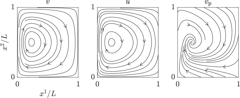
Figure 3: Streamlines of the Stommel wind-driven circulation model velocity (left), the $\delta$-weighted velocity resulting from this velocity and the wind field that drives the Stommel gyre (middle), and dominant part of inertial particle velocity on the slow manifold of the Maxey–Riley set resulting from feeding the later with the aforementioned sewater and air velocities (right).

We first do this by considering as in Beron-Vera, Olascoaga, and Lumpkin (2016) the conceptual model of wind-driven circulation due to Stommel (1948). The steady flow in such a barotropic model is quasigeostrophic, i.e., $v=\nabla^{\perp}\psi(x)=O(\mathrm{Ro})$, and has an anticyclonic basin-wide gyre in the northern hemisphere, so $\omega=\nabla^{2}\psi\leq 0$, driven by steady westerlies and trade winds, namely, $v_{\mathrm{a}}=W(x^{2})e_{1}$ with $W^{\prime}(x^{2})\geq 0$. The leading-order contribution to inertial particle velocity on the slow manifold (53) takes the form

$$v_{\mathrm{p}}=(1-\alpha)\nabla^{\perp}\psi+\alpha We_{1}+\tau f_{0}\big{(}(1-R-\alpha)\nabla\psi+\alpha We_{2}\big{)}$$ (57)

with an $O(\mathrm{R_{0}}^{2})$ error. The divergence of this velocity,

$$\nabla\cdot v_{\mathrm{p}}=\tau f_{0}\big{(}(1-R-\alpha)\nabla^{2}\psi-\alpha W^{\prime}(x^{2})\big{)}.$$ (58)

Recalling that $1-R(\delta)\geq\alpha(\delta)\geq 0$, it follows that $\nabla\cdot v_{\mathrm{p}}\leq 0$, which promotes attraction of inertial particles toward the interior of the gyre in a manner akin to undrogued drifters and plastic debris.

A precise localization of the attractor can be attained by inspecting the streamfunction and the wind field. A simple expression for the streamfuction is Haidvogel and Bryan (1992)

$$\psi=\frac{\pi F}{H\beta}\Big{(}1-x^{1}/L-\mathrm{e}^{-\frac{x^{1}}{r/\beta}}\Big{)}\sin\frac{\pi x^{2}}{L},$$ (59)

where $H$ is the (thermocline) depth, $r$ is the (bottom) friction coefficient, $L$ here is the length of a square domain, and $F$ is the wind stress (per unit density) amplitude, which sets the amplitude of the wind field:

$$W=\operatorname*{sign}\left(x^{2}-\tfrac{1}{2}L\right)\sqrt{\frac{\rho F}{\rho_{\mathrm{a}}C_{\mathrm{D}}}}\sqrt{\operatorname*{sign}\left(\tfrac{1}{2}L-x^{2}\right)\cos\frac{\pi x^{2}}{L}},$$ (60)

where $C_{\mathrm{D}}$ is a (dimensionless) drag coefficient. (We note that $W$ is $C^{\infty}$ everywhere except at $x^{2}=\frac{1}{2}L$, a set of measure zero. Thus (57) is a valid approximation to (29) almost everywhere in the domain.) Figure 3 shows streamlines of $v=\nabla^{\perp}\psi$ on the left, $u=(1-\alpha)\nabla^{\perp}\psi+\alpha We_{1}$ in the middle, and $v_{\mathrm{p}}$ given by (57) on the right. Parameters for the Stommel model are taken as in Stommel (1948) with $C_{\mathrm{D}}=1.2\times 10^{-3}$ (e.g., Large and Pond (1981)). Soft inertial parameters are chosen to represent undrogued GDP drifters, namely, $\delta=2$ and $a=17.5$ cm. We have set also $k=1=k_{\mathrm{a}}$. The rest of the parameters are hard, typical seawater and air values. This gives $R=0.6$ and $\tau=0.0968$ d. Variations of the soft parameters do not change the qualitative aspects of the solution. The streamlines of $v$ show a center, displaced westward, resulting from the $\beta$ effect. The streamlines of $u$ are similar, with a center in precisely the same place. This is located at $(x^{1},x^{2})=(-\smash{\frac{r}{\beta}}\log\smash{\frac{r}{\beta L}},\frac{1}{2}L)$. The stability type of this equilibrium is changed to a stable spiral when the inertial velocity is $v_{\mathrm{p}}$ considered. (Indeed, we have numerically verified that, at that point, $\nabla v$ and $\nabla u$ both have complex conjugate pure imaginary eigenvalues, while the complex conjugate eigenvalue pair of $\nabla v_{\mathrm{p}}$ has a negative real part.) This thus shows explicitly where inertial particles accumulate and further that finite-size effects, produced by the term proportional to $\tau$ in $v_{\mathrm{p}}$, are responsible for driving the accumulation. A search-and-rescue type model, i.e., one for which $\dot{x}=u$ neglecting those effects, is not enough to realize it, as Beron-Vera, Olascoaga, and Lumpkin (2016) noted earlier.

We finalize the Stommel model analysis by comparing the divergence of the inertial velocity (58) with that one that would result from the wind stress curl (Ekman divergence), namely,

$$\nabla\cdot v_{\mathrm{E}}=-\frac{\pi F}{f_{0}HL}\sin\frac{\pi x^{2}}{L},$$ (61)

which is nonpositive. The comparison in presented in Figure 4. Note that $|\nabla\cdot v_{\mathrm{p}}|$ dominates over $|\nabla\cdot v_{\mathrm{E}}|$ in the domain (left panel) while both are much smaller than $f_{0}$ (right panel), reason for which the Ekman convergence does not enter in the Stommel model (it is a higher-order effect in the Rossby number Ro). It is important to realize that the divergence $\smash{\overline{\nabla\cdot v_{\mathrm{p}}}^{1}/f_{0}}$ at $x^{2}=\smash{\frac{1}{2}}L$ is not a deficiency of the Maxey–Riley description of inertial effects, but rather a consequence of the convenient form of the wind stress assumed by Stommel in his model, which leads to a divergence of the associated wind there.

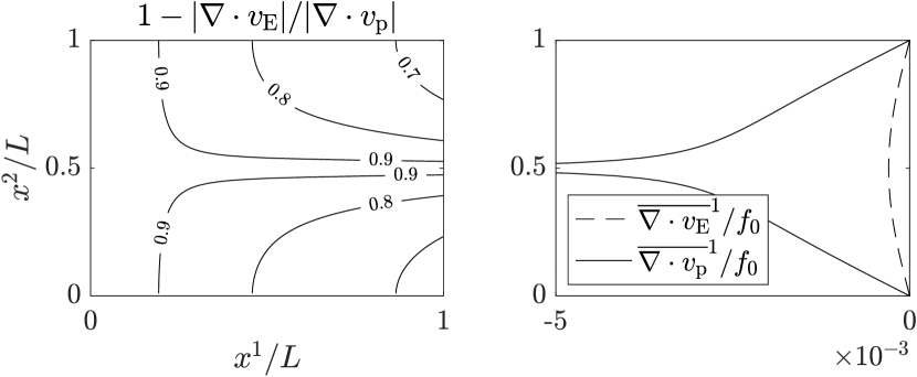
Figure 4: For the Stommel model, relative difference of inertial and Ekman divergence magnitudes (left) and zonally averaged inertial and Ekman divergences normalized by the Coriolis parameter (right).

We now proceed to test the ability of the Maxey–Riley set derived here to promote inertial particle concentration in the subtropical gyres in a realistic setting following Beron-Vera, Olascoaga, and Lumpkin (2016). We focus on the North Atlantic for simplicity as subtropical gyres in the other oceans behave similarly. The exception is the Indian Ocean, where aggregation of inertial particles is not so evident, suggesting that ocean and atmospheric conditions are peculiar there van der Mheen, Pattiaratchi, and van Sebille (2019); Miron et al. (2019a).

Thus we feed the full spherical form of the Maxey–Riley set (A.6) with $v$ as given by surface ocean velocity from the Global $1/12^{\circ}$ HYCOM (HYbrid-Coordinate Ocean Model) $+$ NCODA (Navy Coupled Ocean Data Assimilation) Ocean Reanalysis Cummings and Smedstad (2013), and $v_{\mathrm{a}}$ as the wind velocity from the National Centers for Environmental Prediction (NCEP) Climate Forecast System Reanalysis (CFSR) employed to construct the wind stress applied on the model. (To be more precise, the NCEP winds are provided at 10 m, so we multiply them by one half following Hsu, Meindl, and Gilhousen (1994) to infer $v_{\mathrm{a}}$.) This way ocean currents and winds are made dynamically consistent with each other.

Specifically, we partition the North Atlantic domain into $5^{\circ}\times 5^{\circ}$ longitude–latitude boxes and construct a matrix of probabilities, $P$, of the drifters and the inertial particles to transitioning, irrespective of the start time, among them over a short time. Such a time-independent $P$ represents a discrete autonomous transfer operator which governs the evolution of tracer probability densities, satisfying a stationary advection–diffusion process, on a Markov chain defined on the boxes of the partition Froyland, Stuart, and van Sebille (2014); Miron et al. (2017, 2019b, 2019a); Olascoaga et al. (2018). Thus given an initial probability vector $\mathbf{f}$, this is forward evolved under left multiplication by $P$, namely, $\mathbf{f}_{n}=\mathbf{f}P^{n}$, $n=1,2,\dotsc$. This way long-term evolution can be investigated in a probabilistic sense without the need of long trajectory records, which may be generated numerically but are not available from observations. To construct $P$ we set a transition time of 5 days, which is longer than the Lagrangian decorrelation time scale, estimated to be of the order of 1 day near the ocean surface LaCasce (2008), thereby guaranteeing sufficiently negligible memory into the past that the Markov assumption can be expected to hold well.

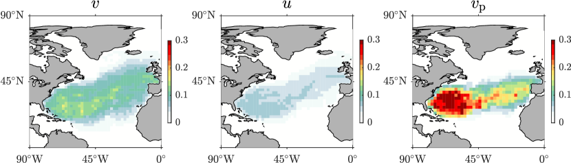
Figure 5: Long-term distribution in the North Atlantic of an initially uniform probability density under action of an autonomous transfer operator constructed using short-run trajectories produced by surface HyCOM velocity (left), $\delta$-weighted velocity where seawater velocity is the HyCOM and the air velocity is the NCP wind used to force HyCOM (middle), and trajectories produced by the Maxey–Riley set derived in this paper fed with these seawater and air velocities (right). Soft inertial parameters choices are $\delta=2$ and $a=17.5$ cm, representing undrogued GDP drifters, and $k=1=k_{\mathrm{a}}$. Densities are subjected to a fourth-root transformation.

Figure 5 shows distributions in the North Atlantic after 10 years of an initially uniform probability density evolving under the action of transition matrix constructed using trajectories produced by HyCOM surface ocean velocity output (left), trajectories of the $\delta$-weighted velocity $u$ resulting from setting $v$ to be the HyCOM velocity and $v_{\mathrm{a}}$ to be the NCEP winds used to force the model (middle), and trajectories produced by the Maxey–Riley set fed with these velocities. (The full spherical form (A.6) of the set is employed in these calculations; trajectories of $v$ and $u$ are computed by integrating the left set in (A.3) with $v_{\mathrm{f}}$ replaced by $v$ and $u$, respectively.) Parameters were taken as above to represent undrogued GDP drifters, $\delta=2$ and $a=17.5$ cm. Note the good qualitative agreement with the results based on the conceptual wind-driven circulation model of Stommel of Figure 3. Note the density values, which are subjected to a fourth-root transformation. Inertial particles reveal accumulation toward the center of the gyre, while seawater particles and particles evolving under the $\delta$-weighted velocity $u$ do not. Indeed, the densities corresponding to the latter are low and distributed more homogeneously over the gyre. Garbage patches in the ocean tend to localize in the center of the gyres consistent with the inertial particles. These reinforces the idea put forth by Beron-Vera, Olascoaga, and Lumpkin (2016) that inertial effects dominate the production of such patches. Ekman transport convergence, the only mechanism acting in the absence of inertial effects, does not control garbage accumulation despite earlier Maximenko, Hafner, and Niiler (2012) and recent van der Mheen, Pattiaratchi, and van Sebille (2019) claims. Furthermore, ignoring finite-size effects results in strong dispersion by view of the very low density values attained. This questions the validity of the leeway modeling framework. The results based on the slow manifold reduction of the Maxey–Riley set are indistinguishable from those based on the full set, which was $v$-initialized with mean HyCOM velocity. This provides support for the validity of the slow manifold reduction.

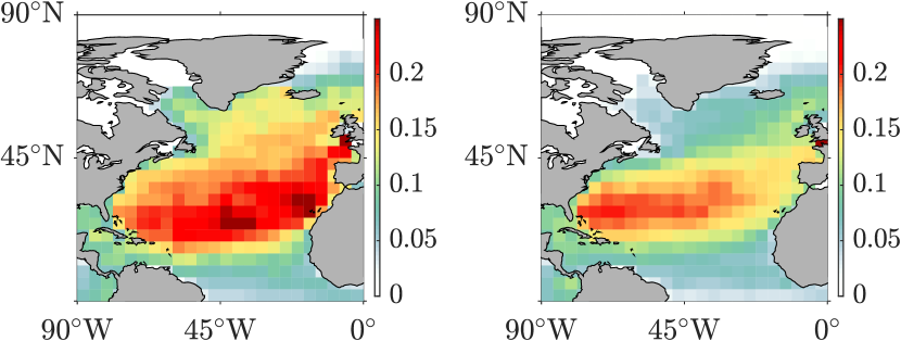
Figure 6: Long-term distribution in the North Atlantic of an initially uniform probability density under action of an autonomous transfer operator constructed using short-run drogued (left) and undrogued (right) trajectories of satellite-tracked drifting buoys from the NOAA Global Drifter Program. Densities are subjected to a fourth-root transformation

Finally, Figure 6 shows the distribution of an initially uniform probability density after 10 years of forward evolution under a discrete action of a transfer operator constructed using drogued (left) and undrogued (right) drifter trajectories from the GDP dataset. Note how undrogued drifter density in the long run tends to concentrate in the center of the gyre more evidently than drogued drifter density. Such a difference was not noted in previous work van Sebille, England, and Froyland (2012); Maximenko, Hafner, and Niiler (2012) which also used probabilistic approaches to investigate long-term behavior. Very importantly, note that this behavior resembles quite well the simulated behavior described above, providing a reality check for it. More specifically, the drogued drifters behave in a manner akin to seawater particles. The undrogued drifters, by contrast, behave more like inertial particles, which represent a prototype for flotsam in general as undrogued drifters and plastic debris present a similar tendency to aggregate in the interior of the subtropical gyres.

VI Concluding remarks

In this paper we have proposed a theory for the motion finite-size particles floating at the ocean surface based on the Maxey–Riley set, the de-jure fluid dynamics framework for inertial particle motion investigation. The theory thus consist of a Maxey–Riley set obtained by vertically averaging the various forces involved in the original Maxey–Riley set, appropriately adapted to account for planet’s rotation and sphericity effects, across an assumed small spherical particle that floats at a flat air–sea interface and thus is subjected to the action ocean currents and winds.

The inertial particle velocity of the resulting Maxey–Riley set is shown to decay exponentially fast in time to a limit that is $O(a^{2})$-close, where $a$ is the particle radius, to an average of the seawater and air velocities weighted by a function of the seawater-to-particle density ratio. This weighted average velocity has a form which is similar to the so-called leeway velocity that forms the basis for search-and-rescue modeling. Such a leeway model is not sufficient to explain the role of mesoscale eddies as traps for marine debris or the formation of garbage patches in subtropical gyres, which are phenomena dominated by finite-size effects.

The resulting Maxey–Riley set either outperforms or has potential for outperforming an earlier proposed set Beron-Vera, Olascoaga, and Lumpkin (2016) in various aspects. For instance, in the neutrally buoyant case, inertial particle motion is synchronized with seawater (i.e., Lagrangian) particle motion under the same conditions as in the original Maxey–Riley set without Coriolis and lift forces. Also, the newly proposed set predicts concentration of particles inside anticyclonic mesoscale eddies consistent with observations of marine microplastic debris. On the other hand, including lift force the new Maxey–Riley set is expected to better represent particle dispersion in the presence of fast submesoscale eddy motion. Furthermore, the proposed heuristic shape corrections raise the earlier set limitation to spherical particles. Finally, recommendations were made for accounting for Stokes drift effects are expected to improve the earlier set performance in the presence of waves, and for incorporating the effects of inhomogeneities of the carrying density field, which can be consequential near frontal regions.

We close by noting that a paper in preparation Olascoaga et al. (2019) reports on the results from a field experiment which involved the deployment, in the Gulf Stream and other areas of the North Atlantic, and subsequently tracking, using global satellite positioning, of buoys of varied buoyancies, sizes, and shapes. In that paper the Maxey–Riley set derived here is shown capable of reproducing individual trajectories with unexpected accuracy given the uncertainty around the ocean current and wind representations, providing strong support the validity of the set.

Appendix A Inertial ocean dynamics on the sphere

Let $a_{\odot}$ be the mean radius of the Earth, and consider the rescaled longitude ($\lambda$) and latitude ($\vartheta$) coordinates, namely,

$$x^{1}=(\lambda-\lambda_{0})\cdot a_{\odot}\cos\vartheta_{0},\quad x^{2}=(\vartheta-\vartheta_{0})\cdot a_{\odot},$$ (A.1)

respectively, measured from an arbitrary location on the surface of the planet. Consider further the following geometric coefficients Ripa (1997a):

$$\gamma_{\odot}:=\sec\vartheta_{0}\cos\vartheta,\quad\tau_{\odot}:=a_{\odot}^{-1}\tan\vartheta.$$ (A.2)

The (horizontal) velocity of a fluid particle and its acceleration as measured by a terrestrial observer are (cf. Ripa (1997a); Beron-Vera (2003))

$$v_{\mathrm{f}}=\begin{pmatrix}\gamma_{\odot}&0\\ 0&1\end{pmatrix}\dot{x},\quad a_{\mathrm{f}}=\dot{v}_{\mathrm{f}}+(f+\tau_{\odot}v_{\mathrm{f}}^{1})v_{\mathrm{f}}^{\perp},$$ (A.3)

respectively, where $f=2\Omega\sin\vartheta$. It is important to realize that this is not a mere change of coordinates from Cartesian to spherical. Very differently, this is a consequence of the gravitational force, which, attracting the particle to the nearest pole, is required to sustain a steady rotation, with angular velocity $\pm\Omega$, relative to a fixed frame, at any point on the planet’s surface. The terrestrial observer is then left with just the Coriolis force, in the absence of any other forces, to describe motion on the surface of the Earth. A very enlightening way to derive the formula for the acceleration in (A.3) is from Hamilton’s principle, with the Lagrangian as written by an observer standing in a fixed frame, so the only force acting on the particle (in the absence of any other forces) is the gravitational one, and the coordinates employed by this observer related to those rotating with the planet (A.1) (cf. Ripa (1997a); Beron-Vera (2003)). This is in essence what Pierre Simon de Laplace (1749–1827) did to derive his theory of tides and at the same time discover the Coriolis force over a quarter of a century before Gaspard Gustave de Coriolis (1792–1843) was born Ripa (1995). For a nice account on the history of this, many times misunderstood, force, cf. Ripa (1997b).

By a similar token, the fluid’s Eulerian acceleration takes the form

$$\frac{\operatorname{D}\!{v_{\mathrm{f}}}}{\operatorname{D}\!{t}}+(f+\tau_{\odot}v_{\mathrm{f}}^{1})v_{\mathrm{f}}^{\perp},$$ (A.4)

where

$$\frac{\operatorname{D}\!{v_{\mathrm{f}}}}{\operatorname{D}\!{t}}=\partial_{t}v_{\mathrm{f}}+(\nabla v_{\mathrm{f}})\dot{x}=\partial_{t}v_{\mathrm{f}}+(\gamma_{\odot}^{-1}\partial_{1}v_{\mathrm{f}})v_{\mathrm{f}}^{1}+(\partial_{2}v_{\mathrm{f}})v_{\mathrm{f}}^{2}.$$ (A.5)

Equations hold for a particle of fluid, either seawater or air, and also for an inertial particle. The acceleration of the inertial particle on the left-hand-side of (yet to be evaluated) Maxey–Riley set (21) and in the added mass force (14) is the $\beta$-plane form of $a_{\mathrm{f}}$ in (A.3) for the case of an inertial particle, resulting from making $\gamma_{\odot}=1$, $\tau_{\odot}=0$, and $f=f_{0}+\beta x^{2}$, which, despite its wide used, does not represent a consistent leading order in $|x^{2}|/a_{\odot}\ll 1$ approximation Ripa (1997a). In turn, the fluid’s Eulerian acceleration that appears in the flow force (13) and the added mass term (14) is the $\beta$-plane form of (A.4)–(A.5).

With the above in mind, the Maxey–Riley set (29) on the sphere then takes the form

$$\dot{v}_{\mathrm{p}}+\left(f+\tau_{\odot}v_{\mathrm{p}}^{1}+\tfrac{1}{3}R\omega\right)v_{\mathrm{p}}^{\perp}+\tau^{-1}v_{\mathrm{p}}=R\frac{\operatorname{D}\!{v}}{\operatorname{D}\!{t}}+R\left(f+\tau_{\odot}v^{1}+\tfrac{1}{3}\omega\right)v^{\perp}+\tau^{-1}u,$$ (A.6)

with $\frac{\operatorname{D}\!{}}{\operatorname{D}\!{t}}v$ given by (A.5) and

$$\omega=\gamma_{\odot}^{-1}\partial_{1}v^{2}-\gamma_{\odot}^{-1}\partial_{2}(\gamma_{\odot}v^{1})=\gamma_{\odot}^{-1}\partial_{1}v^{2}-\partial_{2}v^{1}+\tau_{\odot}v^{1}$$ (A.7)

as it follows from its definition, $\omega:=\smash{\lim_{\Delta x^{1}\Delta x^{2}\to 0}}\smash{\frac{1}{\gamma_{\odot}\Delta x^{1}\Delta x^{2}}}\smash{\oint}(\gamma_{\odot}v^{1}\operatorname{d}\!{x^{1}}+v^{2}\operatorname{d}\!{x^{2}})$, and noting that $\gamma_{\odot}^{\prime}(x^{2})/\gamma_{\odot}(x^{2})=-\tau_{\odot}(x^{2})$

Applying the slow-manifold reduction on (A.6) it follows, to leading order on the slow manifold, that

$$\dot{x}\sim u+\tau\bigg{(}R\frac{\operatorname{D}\!{v}}{\operatorname{D}\!{t}}+R\left(f+\tau_{\odot}v^{1}+\tfrac{1}{3}\omega\right)v^{\perp}-\frac{\operatorname{D}\!{u}}{\operatorname{D}\!{t}}-\left(f+\tau_{\odot}v^{1}+\tfrac{1}{3}R\omega\right)u^{\perp}\bigg{)},$$ (A.8)

where $\frac{\operatorname{D}\!{}}{\operatorname{D}\!{t}}u$ is as in (A.5) with $v_{\mathrm{f}}$ replaced by $u$.

Appendix B Attractivity and instability conditions for neutrally buoyant particles

To derive an attractivity condition for $\mathcal{N}$ in the present geophysical setting ($f\neq 0$) with lift force, we follow Sapsis and Haller (2008) closely by first fixing a solution $(y,x)(t)$ to (34), which fixes $A(x(t),t)$. Then noting that $y^{\top}Ay=y^{\top}(rA+(1-r)A^{\top})y$ for any $r\in\mathbb{R}$, one finds, using $r=\frac{1}{2}$, that $y^{\top}Ay\leq\max\operatorname*{spec}\smash{\frac{A+A^{\top}}{2}}\cdot|y|^{2}$, which follows from real symmetric $A+A^{\top}$ admitting an orthogonal diagonalization. Now, taking into account that $J=-J^{\top}$,

$$\frac{A+A^{\top}}{2}=S+\tau^{-1}\operatorname{Id}$$ (B.1)

and hence

$$\frac{1}{2}\frac{\operatorname{d}\!{}}{\operatorname{d}\!{t}}|y|^{2}=-y^{\top}(S+\tau^{-1}\operatorname{Id})y\leq-\min\operatorname*{spec}(S+\tau^{-1}\operatorname{Id})\cdot|y|^{2}.$$ (B.2)

Integrating from $t=t_{0}$ to $t>t_{0}$,

$$|y(t)|^{2}\leq|y(t_{0})|^{2}\mathrm{e}^{\textstyle{-\int_{t_{0}}^{t}(S(x(s),s)+\tau^{-1}\operatorname{Id})\operatorname{d}\!{s}}}.$$ (B.3)

Then for $|y(t)|$ to decay from $|y(t_{0})|$ as $t$ increases, it is sufficient that the integrand in (B.3) be positive for all $x\in D$ over the time interval $I$, from which the global attractivity condition (36) follows.

As noted by Sapsis and Haller (2008), perturbations off $\mathcal{N}$ which are initially sufficiently small will grow or decay depending on the sign of the instantaneous stability indicator

$$\Lambda(x_{0},t_{0})=\lim_{t\to t_{0}}\smash{\frac{2}{t-t_{0}}}\log||P_{t_{0}}^{t}||_{2}$$ (B.4)

Here $P_{t_{0}}^{t}$ satisfies

$$\dot{P}_{t_{0}}^{t}=A(x(t;t_{0},x_{0}),t)P_{t_{0}}^{t},\quad P_{t_{0}}^{t_{0}}=\operatorname{Id},$$ (B.5)

so $y(t;t_{0},y_{0},x_{0})=P_{t_{0}}^{t}y_{0}$, to wit, $P_{t_{0}}^{t}$ represents the fundamental matrix solution of (34) for initial condition $(y,x)(t_{0})=(y_{0},x_{0})$. Taylor expanding $P_{t_{0}}^{t}$ one finds

$$P_{t_{0}}^{t}=\operatorname{Id}+A_{0}\cdot(t-t_{0})+O((t-t_{0})^{2}),$$ (B.6)

where the shorthand notation $A_{0}=A(t_{0})$ is used, and hence

$$(P_{t_{0}}^{t})^{\top}P_{t_{0}}^{t}=\operatorname{Id}+(A_{0}+A_{0}^{\top})\cdot(t-t_{0})+O((t-t_{0})^{2}).$$ (B.7)

Then

$$(||P_{t_{0}}^{t}||_{2})^{2}=1-2\min\operatorname*{spec}(S_{0}+\tau^{-1}\operatorname{Id})\cdot(t-t_{0})+O((t-t_{0})^{2}),$$ (B.8)

where (B.1) was used. Now, using $\log\left(1+\smash{\sum_{1}^{\infty}}c_{n}\varepsilon^{n}\right)=c_{1}\varepsilon+O(\varepsilon^{2})$ for $\varepsilon>0$ small, one finds

$$\Lambda(x_{0},t_{0})=-2\min\operatorname*{spec}(S(x_{0},t_{0})+\tau^{-1}\operatorname{Id}).$$ (B.9)

Replacing $(x_{0},t_{0})$ with $(x(t),t)$, it follows that instantaneous divergence away from $\mathcal{N}$ will take place where $S+\tau^{-1}\operatorname{Id}$ is sign indefinite, or, equivalently, where (36) is violated.

Appendix C Slow manifold reduction in the standard fluid mechanics setting with lift force

The standard fluid mechanics Maxey–Riley equation with lift force is given by (cf. Montabone (2002), Chapter 4)

$$\dot{v}_{\mathrm{p}}+\tfrac{1}{2}R\omega v_{\mathrm{p}}^{\perp}+\tau^{-1}v_{\mathrm{p}}=\tfrac{3}{2}R\frac{\operatorname{D}\!{v}}{\operatorname{D}\!{t}}+\tfrac{1}{2}R\omega v^{\perp}+\tau^{-1}v,$$ (C.1)

where $v$ is any carrying flow velocity and

$$\tau:=\frac{2R}{9}\cdot\frac{a^{2}}{\mu/\rho},\quad R:=\frac{2\delta}{2+\delta}.$$ (C.2)

In nondimensional variables with time rescaled as in §4, the above equation in system form reads

$$x^{\prime} =\tau v_{\mathrm{p}},$$ (C.3)

$$\varphi^{\prime} =\tau,$$ (C.4)

$$v_{\mathrm{p}}^{\prime} =v-v_{\mathrm{p}}-\tfrac{1}{2}\tau R\omega v_{\mathrm{p}}^{\perp}+\tfrac{3}{2}\tau R\smash{\frac{\operatorname{D}\!{v}}{\operatorname{D}\!{t}}}+\tfrac{1}{2}\tau R\omega v^{\perp}.$$ (C.5)

The critical manifold for the above system is

$$\mathcal{S}_{0}=\{(x,\varphi,v_{\mathrm{p}})\mid v_{\mathrm{p}}=v(x,\varphi),\ x\in D,\,\varphi\in I\},$$ (C.6)

so the slow manifold takes the form:

$$\mathcal{S}_{\tau}:=\{(x,\varphi,v_{\mathrm{p}})\mid v_{\mathrm{p}}=v(x,\varphi)+\sum\nolimits_{1}^{r}\tau^{n}v_{n}(x,\varphi)+O(\tau^{r+1}),\ (x,\varphi)\in D\times I\}.$$ (C.7)

Differentiating the equation defining $\mathcal{S}_{\tau}$ above with respect to $\mathfrak{t}$,

$$v_{\mathrm{p}}^{\prime}={} \left[(\nabla v)x^{\prime}+\partial_{\varphi}v\varphi^{\prime}+\sum\nolimits_{1}^{r}\tau^{n}\big{(}(\nabla v_{n})x^{\prime}+\partial_{\varphi}v_{n}\varphi^{\prime}\big{)}+O(\tau^{r+1})\right]_{\mathcal{S}_{\tau}}$$

$$={} \tau\frac{\operatorname{D}\!{v}}{\operatorname{D}\!{t}}+\sum\nolimits_{n=2}^{r}\tau^{n}\Big{(}\partial_{t}v_{n-1}+(\nabla v_{n-1})v+(\nabla v)v_{n-1}$$

$$+\sum\nolimits_{m=1}^{n-2}(\nabla v_{m})v_{n-m-1}\Big{)}+O(\tau^{r+2}).$$ (C.8)

Then restricting (C.5) to $\mathcal{S}_{\tau}$, i.e.,

$$v_{\mathrm{p}}^{\prime}={} \Big{[}v-v_{\mathrm{p}}-\tfrac{1}{2}\tau R\omega v_{\mathrm{p}}^{\perp}+\tfrac{3}{2}\tau R\smash{\frac{\operatorname{D}\!{v}}{\operatorname{D}\!{t}}}+\tfrac{1}{2}\tau R\omega v^{\perp}\Big{]}_{\mathcal{S}_{\tau}}$$

$$={} -\sum\nolimits_{1}^{r}\tau^{n}v_{n}-\tfrac{1}{2}\tau R\omega\left(v^{\perp}+\sum\nolimits_{1}^{r}\tau^{n}v_{n}^{\perp}\right)+\tfrac{3}{2}\tau R\smash{\frac{\operatorname{D}\!{v}}{\operatorname{D}\!{t}}}$$

$$+\tfrac{1}{2}\tau R\omega v^{\perp}+O(\tau^{r+2}),$$ (C.9)

and equating equal $\tau$-power terms in (C.8) and (C.9), we obtain

$$v_{1}={} \left(\tfrac{3}{2}R-1\right)\frac{\operatorname{D}\!{v}}{\operatorname{D}\!{t}}$$ (C.10)

$$v_{n}={} -\tfrac{1}{2}R\omega v_{n-1}^{\perp}$$

$$-\partial_{t}v_{n-1}-(\nabla v_{n-1})v-(\nabla v)v_{n-1}$$

$$-\sum\nolimits_{m=1}^{n-2}(\nabla v_{m})v_{n-m-1},\quad n\geq 2.$$ (C.11)

The Maxey–Riley set (C.1) on the slow manifold $\mathcal{S}_{\tau}$ reduces to

$$\dot{x}=v_{\mathrm{p}}=v(x,t)+\sum\nolimits_{1}^{r}\tau^{n}v_{n}(x,t)+O(\tau^{r+1})$$ (C.12)

with $v_{n}(x,t)$ as given in (C.10)–(C.11). Note that the lift force makes an $O(\tau^{2})$ contribution to $\mathcal{S}_{\tau}$.

References

- Stokes (1851) G. G. Stokes, “On the Effect of the Internal Friction of Fluids on the Motion of Pendulums,” Transactions of the Cambridge Philosophical Society 9, 8 (1851).
- Basset (1888) A. B. Basset, “Treatise on hydrodynamics,” (Deighton Bell, London, 1888) Chap. 22, pp. 285–297.
- Boussinesq (1885) J. V. Boussinesq, “Sur la résistance quóppose un fluide indéfini au repos, sans pesanteur, au mouvement varié dúne sphére solide qu’il mouille sur toute sa surface, quand les vitesses restent bien continues et assez faibles pour que leurs carrés et produits soient négligeables,” Comptes Rendu de l’Academie des Sciences 100, 935–937 (1885).
- Oseen (1927) C. W. Oseen, Hydrodynamik (Akademische Verlagsgesellschaft, Leipzig, 1927).
- Tchen (1947) C. M. Tchen, Ph.D. thesis, Delft, Martinus Nijhoff, The Hage (1947).
- Corrsin and Lumely (1956) S. Corrsin and J. Lumely, Appl. Sci. Res. A 6, 114 (1956).
- Maxey and Riley (1983) M. R. Maxey and J. J. Riley, “Equation of motion for a small rigid sphere in a nonuniform flow,” Phys. Fluids 26, 883 (1983).
- Riley (1971) J. J. Riley, Ph.D. thesis, The John Hopkins University, Baltimore, Maryland (1971).
- Gatignol (1983) R. Gatignol, “The faxen formulae for a rigid particle in an unsteady non-uniform stokes flow,” J. Mec. Theor. Appl. 1, 143–160 (1983).
- Auton, Hunt, and Prud’homme (1988) T. R. Auton, F. C. R. Hunt, and M. Prud’homme, “The force exerted on a body in inviscid unsteady non-uniform rotational flow,” J. Fluid. Mech. 197, 241 (1988).
- Michaelides (1997) E. E. Michaelides, “Review—The transient equation of motion for particles, bubbles and droplets,” ASME. J. Fluids Eng. 119, 233–247 (1997).
- Provenzale (1999) A. Provenzale, “Transport by coherent barotropic vortices,” Annu. Rev. Fluid Mech. 31, 55–93 (1999).
- Cartwright et al. (2010) J. H. E. Cartwright, U. Feudel, G. Károlyi, A. de Moura, O. Piro, and T. Tél, “Dynamics of finite-size particles in chaotic fluid flows,” in Nonlinear Dynamics and Chaos: Advances and Perspectives, edited by M. Thiel et al. (Springer-Verlag Berlin Heidelberg, 2010) pp. 51–87.
- Babiano et al. (2000) A. Babiano, J. H. Cartwright, O. Piro, and A. Provenzale, “Dynamics of a small neutrally buoyant sphere in a fluid and targeting in Hamiltonian systems,” Phys. Rev. Lett. 84, 5,764–5,767 (2000).
- Vilela, de Moura, and Grebogi (2006) R. D. Vilela, A. P. S. de Moura, and C. Grebogi, “Finite-size effects on open chaotic advection,” Phys. Rev. E 73, 026302 (2006).
- Breivik et al. (2013) Ø. Breivik, A. A. Allen, C. Maisondieu, and M. Olagnon, “Advances in search and rescue at sea,” Ocean Dynamics 63, 83–88 (2013).
- Bellomo et al. (2015) L. Bellomo, A. Griffa, S. Cosoli, P. Falco, R. Gerin, I. Iermano, A. Kalampokis, Z. Kokkini, A. Lana, M. Magaldi, I. Mamoutos, C. Mantovani, J. Marmain, E. Potiris, J. Sayol, Y. Barbin, M. Berta, M. Borghini, A. Bussani, L. Corgnati, Q. Dagneaux, J. Gaggelli, P. Guterman, D. Mallarino, A. Mazzoldi, A. Molcard, A. Orfila, P.-M. Poulain, C. Quentin, J. Tintoré, M. Uttieri, A. Vetrano, E. Zambianchi, and V. Zervakis, “Toward an integrated hf radar network in the mediterranean sea to improve search and rescue and oil spill response: the tosca project experience,” Journal of Operational Oceanography 8, 95–107 (2015).
- Gower and King (2008) J. Gower and S. King, “Satellite images show the Movement of floating Sargassum in the Gulf of Mexico and Atlantic Ocean,” Available from Nature Precedings (http://hdl.handle.net/10101/npre.2008.1894.1) (2008).
- Brooks, Coles, and Coles (2019) M. T. Brooks, V. J. Coles, and W. C. Coles, “Inertia influences pelagic sargassum advection and distribution,” Geophysical Research Letters 46, 2610–2618 (2019).
- Law et al. (2010) K. L. Law, S. Morét-Ferguson, N. A. Maximenko, G. Proskurowski, E. E. Peacock, J. Hafner, and C. M. Reddy, “Plastic accumulation in the North Atlantic subtropical gyre,” Science 329, 1185–1188 (2010).
- Cozar et al. (2014) A. Cozar, F. Echevarria, J. I. Gonzalez-Gordillo, X. Irigoien, B. Ubeda, S. Hernandez-Leon, A. T. Palma, S. Navarro, J. Garcia-de Lomas, R. andrea, M. L. Fernandez-de Puelles, and C. M. Duarte, “Plastic debris in the open ocean,” Proc. Nat. Acad. Sci. USA 111, 10239–10244 (2014).
- Trinanes et al. (2016) J. A. Trinanes, M. J. Olascoaga, G. J. Goni, N. A. Maximenko, D. A. Griffin, and J. Hafner, “Analysis of flight MH370 potential debris trajectories using ocean observations and numerical model results,” Journal of Operational Oceanography 9, 126–138 (2016).
- Miron et al. (2019a) P. Miron, F. J. Beron-Vera, M. J. Olascoaga, and P. Koltai, “Markov-chain-inspired search for MH370,” Chaos: An Interdisciplinary Journal of Nonlinear Science 29, 041105 (2019a).
- Rypina et al. (2013) I. Rypina, S. R. Jayne, S. Yoshida, A. M. Macdonald, E. Douglas, and K. Buesseler, “Short-term dispersal of Fukushima-derived radionuclides off Japan: modeling efforts and model-data intercomparison,” Biogeosciences 10, 4973–4990 (2013).
- Matthews et al. (2017) J. P. Matthews, L. Ostrovsky, Y. Yoshikawa, S. Komori, and H. Tamura, “Dynamics and early post-tsunami evolution of floating marine debris near Fukushima Daiichi,” Nature Geosci. 10, 598–603 (2017).
- Szanyi, Lukovich, and Barber (2016) S. Szanyi, J. V. Lukovich, and D. G. Barber, “Lagrangian analysis of sea-ice dynamics in the arctic ocean,” Polar Research 35, 30778 (2016).
- Nielsen (1994) P. Nielsen, “Suspended sediment particle motion in coastal flows,” Coastal Engineering Proceedings 1, 2406–2416 (1994).
- Reigada et al. (2003) R. Reigada, R. M. Hillary, M. A. Bees, J. M. Sancho, and F. Sagues, “Plankton blooms induced by turbulent flows,” Proc. R. Soc. B: Biological Sciences 270, 875–880 (2003).
- Peng and Dabiri (2009) J. Peng and J. O. Dabiri, “Transport of inertial particles by Lagrangian Coherent Structures: application to predator-prey interaction in jellyfish feeding,” J. Fluid Mech. 623, 75–84 (2009).
- Monroy et al. (2016) P. Monroy, E. Hernández-García, V. Rossi, and C. López, “Modeling the dynamical sinking of biogenic particles in oceanic flow,” (2016).
- Beron-Vera et al. (2015) F. J. Beron-Vera, M. J. Olascoaga, G. Haller, M. Farazmand, J. Triñanes, and Y. Wang, “Dissipative inertial transport patterns near coherent Lagrangian eddies in the ocean,” Chaos 25, 087412 (2015).
- Haller and Beron-Vera (2013) G. Haller and F. J. Beron-Vera, “Coherent Lagrangian vortices: The black holes of turbulence,” J. Fluid Mech. 731, R4 (2013).
- Haller and Beron-Vera (2014) G. Haller and F. J. Beron-Vera, “Addendum to ‘Coherent Lagrangian vortices: The black holes of turbulence’,” J. Fluid Mech. 755, R3 (2014).
- Haller et al. (2016) G. Haller, A. Hadjighasem, M. Farazmand, and F. Huhn, “Defining coherent vortices objectively from the vorticity,” J. Fluid Mech. 795, 136–173 (2016).
- Beron-Vera, Olascoaga, and Lumpkin (2016) F. J. Beron-Vera, M. J. Olascoaga, and R. Lumpkin, “Inertia-induced accumulation of flotsam in the subtropical gyres,” Geophys. Res. Lett. 43, 12228–12233 (2016).
- Maximenko and Niiler (2006) N. A. Maximenko and P. P. Niiler, “Mean surface circulation of the global ocean inferred from satellite altimeter and drifter data,” in 15 years of Progress in Radar Altimetry (ESA Publication SP-614, 2006).
- Brach et al. (2018) L. Brach, P. Deixonne, M.-F. Bernard, E. Durand, M.-C. Desjean, E. Perez, E. van Sebille, and A. ter Halle, “Anticyclonic eddies increase accumulation of microplastic in the north atlantic subtropical gyre,” Marine Pollution Bulletin 126, 191–196 (2018).
- Chelton et al. (2011) D. B. Chelton, P. Gaube, M. G. Schlax, J. J. Early, and R. M. Samelson, “The influence of nonlinear mesoscale eddies on near-surface oceanic chlorophyll,” Science 334, 328–332 (2011).
- Olascoaga et al. (2019) M. J. Olascoaga, F. J. Beron-Vera, U. R. P. Miron, J. Trinanes, R. Lumpkin, and G. J. Goni, “Observation and quantification of inertial effects on the drift of floating objects at the ocean surface,” In prepaparation. (2019).
- Note (1) While having a positive discriminant, the cubic polynomial in (7\@@italiccorr) is irreducible over the reals. Thus while its three roots are real, they require complex numbers to be expressed in radicals Wantzel (1843).
- Auton (1987) T. R. Auton, “The lift force on a spherical body in a rotational flow,” Journal of Fluid Mechanics 183, 199–218 (1987).
- Beron-Vera et al. (2018) F. J. Beron-Vera, A. Hadjighasem, Q. Xia, M. J. Olascoaga, and G. Haller, “Coherent Lagrangian swirls among submesoscale motions,” Proc. Natl. Acad. Sci. U.S.A. Mar 2018, 201701392 (2018).
- Montabone (2002) L. Montabone, Vortex Dynamics and Particle Transport in Barotropic Turbulence, Ph.D. thesis, University of Genoa, Italy (2002).
- Henderson, Gwynllyw, and Barenghi (2007) K. L. Henderson, D. R. Gwynllyw, and C. F. Barenghi, “Particle tracking in Taylor–Couette flow,” European Journal of Mechanics - B/Fluids 26, 738 – 748 (2007).
- Sapsis et al. (2011) T. P. Sapsis, N. T. Ouellette, J. P. Gollub, and G. Haller, “Neutrally buoyant particle dynamics in fluid flows: Comparison of experiments with lagrangian stochastic models,” Physics of Fluids 23, 093304 (2011).
- Farazmand and Haller (2015) M. Farazmand and G. Haller, “The Maxey–Riley equation: Existence, uniqueness and regularity of solutions,” Nonlinear Analysis: Real World Applications 22, 98–106 (2015).
- Langlois, Farazmand, and Haller (2015) G. P. Langlois, M. Farazmand, and G. Haller, “Asymptotic dynamics of inertial particles with memory,” Journal of Nonlinear Science 25, 1225–1255 (2015).
- Daitche and Tél (2011) A. Daitche and T. Tél, “Memory effects are relevant for chaotic advection of inertial particles,” Phys. Rev. Lett. 107, 244501 (2011).
- Daitche and Tél (2014) A. Daitche and T. Tél, “Memory effects in chaotic advection of inertial particles,” New Journal of Physics 16, 073008 (2014).
- Sudharsan, Brunton, and Riley (2016) M. Sudharsan, S. L. Brunton, and J. J. Riley, “Lagrangian coherent structures and inertial particle dynamics,” Phys. Rev. E 93, 033108 (2016).
- Note (2) In an earlier geophysical adaptation of the Maxey–Riley equation Provenzale (1999), the centrifugal force was included as well, but this is actually balanced out by the gravitational force on the horizontal plane.
- Pedlosky (1987) J. Pedlosky, Geophysical Fluid Dynamics, 2nd ed. (Springer, 1987) p. 624 pp.
- Ripa (1997a) P. Ripa, ““Inertial” oscillations and the -plane approximation(s),” J. Phys. Oceanogr. 27, 633–647 (1997a).
- Röhrs et al. (2012) J. Röhrs, K. H. Christensen, L. R. Hole, G. Broström, M. Drivdal, and S. Sundby, “Observation-based evaluation of surface wave effects on currents and trajectory forecasts,” Ocean Dyn. 62, 1519–1533 (2012).
- Nesterov (2018) O. Nesterov, “Consideration of various aspects in a drift study of MH370 debris,” Ocean Sci. 14, 387–402 (2018).
- Sozza et al. (2016) A. Sozza, F. De Lillo, S. Musacchio, and G. Boffetta, “Large-scale confinement and small-scale clustering of floating particles in stratified turbulence,” Physical Review Fluids 1, 052401(R) (2016).
- Breivik and Allen (2008) Ø. Breivik and A. Allen, “An operational search and rescue model for the Norwegian Sea and the North Sea,” J. Marine Syst. 69, 99–113 (2008).
- Duhec et al. (2015) A. V. Duhec, R. F. Jeanne, N. Maximenko, and J. Hafner, “Composition and potential origin of marine debris stranded in the Western Indian Ocean on remote Alphonse Island, Seychelles,” Mar. Poll. Bull. 96, 76–86 (2015).
- Allshouse et al. (2017) M. R. Allshouse, G. N. Ivey, R. J. Lowe, N. L. Jones, C. Beegle-krause, J. Xu, and T. Peacock, “Impact of windage on ocean surface lagrangian coherent structures,” Environmental Fluid Mechanics 17, 473–483 (2017).
- Geyer (1989) W. R. Geyer, “Field calibration of mixed-layer drifters,” Journal of Atmospheric and Oceanic Technology 6, 333–342 (1989), https://doi.org/10.1175/1520-0426(1989)006¡0333:FCOMLD¿2.0.CO;2 .
- Kundu, Cohen, and Dowling (2012) P. K. Kundu, I. M. Cohen, and D. R. Dowling, Fluid Mechanics, 5th ed. (Academic Press, 2012) p. 891.
- Daniel et al. (2002) P. Daniel, G. Jan, F. Cabioc’h, Y. Landau, and E. Loiseau, “Drift modeling of cargo containers,” Spill Science & Technology Bulletin 7, 279 – 288 (2002).
- Ganser (1993) G. H. Ganser, “A rational approach to drag prediction of spherical and nonspherical particles,” Powder Tecnology 77, 143–152 (1993).
- Phillips (1997) O. M. Phillips, Dynamics of the Upper Ocean (Cambridge University Press, 1997).
- Breivik et al. (2015) Ø. Breivik, K. Mogensen, J.-R. Bidlot, M. A. Balmaseda, and P. A. E. M. Janssen, “Surface wave effects in the nemo ocean model: Forced and coupled experiments,” J. Geophys. Res. 120, 2973–2992 (2015).
- Craik (1982) A. D. D. Craik, “The drift velocity of water waves,” J. Fluid Mech. 116, 187–205 (1982).
- Jenkins (1989) A. D. Jenkins, “The use of a wave prediction model for driving a near-surface current model,” Ocean Dyn. 42, 133–149 (1989).
- Webb and Fox-Kemper (2011) A. Webb and B. Fox-Kemper, “Wave spectral moments and Stokes drift estimation,” Ocean Modell. 40, 273–288 (2011).
- Tamura, Miyazawa, and Oey (2012) H. Tamura, Y. Miyazawa, and L.-Y. Oey, “The Stokes drift and wave induced-mass flux in the North Pacific,” J. Geophys. Res. 117, C08021 (2012).
- Breivik, Bidlot, and Janssen (2016) Ø. Breivik, J.-R. Bidlot, and P. A. Janssen, “A Stokes drift approximation based on the Phillips spectrum,” Ocean Modelling 100, 49 – 56 (2016).
- Wu (1983) J. Wu, “Sea-surface drift currents induced by wind and waves,” J. Phys. Oceanogr. 13, 1441–1451 (1983), https://doi.org/10.1175/1520-0485(1983)013¡1441:SSDCIB¿2.0.CO;2 .
- Tanga and Provenzale (1994) P. Tanga and A. Provenzale, “Dynamics of advected tracers with varying buoyancy,” Physica D 76, 202–215 (1994).
- Sapsis and Haller (2008) T. Sapsis and G. Haller, “Instabilities in the dynamics of neutrally buoyant particles,” Physics of Fluids 20, 017102 (2008).
- Rubin, Jones, and Maxey (1995) J. Rubin, C. K. R. T. Jones, and M. Maxey, “Settling and asymptotic motion of aerosol particles in a cellular flow field,” J. Nonlin. Sci. 5, 337–358 (1995), 10.1007/BF01275644.
- Burns, Davis, and Moore (1999) T. J. Burns, R. W. Davis, and E. F. Moore, “A perturbation study of particle dynamics in a plane wake flow,” J. Fluid Mech. 384, 1–26 (1999).
- Mograbi and Bar-Ziv (2006) E. Mograbi and E. Bar-Ziv, “On the asymptotic solution of the Maxey Riley equation,” Phys. Fluids 18, 051704 (2006).
- Haller and Sapsis (2008) G. Haller and T. Sapsis, “Where do inertial particles go in fluid flows?” Physica D 237, 573–583 (2008).
- Fenichel (1979) N. Fenichel, “Geometric singular perturbation theory for ordinary differential equations,” J. Differential Equations 31, 51–98 (1979).
- Jones (1995) C. K. R. T. Jones, “Dynamical Systems, Lecture Notes in Mathematics,” (Springer-Verlag, Berlin, 1995) Chap. Geometric Singular Perturbation Theory, pp. 44–118.
- Note (3) The slow manifold and the Maxey–Riley equation restricted to formally satisfy the definition of inertial manifold and inertial equation, respectively, developed in the study of long-time-asymptotic behavior (attractors) of infinite-dimensional dynamical systems Temam (1990). In such systems, actual attractors are hard to compute and are generally not even manifolds. The inertial manifold is easier to compute, smooth, and contains the attractor. It is unclear to us why these constructs are called “inertial,” but this certainly is not related to resistance of an object to a change in its velocity as meant here.
- Haller and Sapsis (2010) G. Haller and T. Sapsis, “Localized instability and attraction along invariant manifolds,” Siam J. Applied Dynamical Systems 9, 611–633 (2010).
- Roberts (2008) A. J. Roberts, “Normal form transforms separate slow and fast modes in stochastic dynamical systems,” Physica A 387, 12 38 (2008).
- Olascoaga et al. (2016) M. J. Olascoaga, I. I. Rypina, M. G. Brown, F. J. Beron-Vera, H. Koçak, L. E. Brand, G. R. Halliwell, and L. K. Shay, “Persistent transport barrier on the West Florida Shelf,” Geophysical Research Letters 33, L22603 (2016), https://agupubs.onlinelibrary.wiley.com/doi/pdf/10.1029/2006GL027800 .
- Gear and Kevrekidis (2003) C. Gear and I. G. Kevrekidis, “Computing in the past with forward integration,” Phys. Lett. A 321, 335 343 (2003).
- Beron-Vera (2019) F. J. Beron-Vera, “Preferential sampling of elastic inertial chains in the ocean,” Preprint (2019).
- Lumpkin and Pazos (2007) R. Lumpkin and M. Pazos, “Measuring surface currents with Surface Velocity Program drifters: the instrument, its data and some recent results,” in Lagrangian Analysis and Prediction of Coastal and Ocean Dynamics, edited by A. Griffa, A. D. Kirwan, A. Mariano, T. Özgökmen, and T. Rossby (Cambridge University Press, 2007) Chap. 2, pp. 39–67.
- Niiler and Paduan (1995) P. P. Niiler and J. D. Paduan, “Wind-driven Motions in the northeastern Pacific as measured by Lagrangian drifters,” J. Phys. Oceanogr. 25, 2819–2830 (1995).
- Lebreton et al. (2018) L. Lebreton, B. Slat, F. Ferrari, B. Sainte-Rose, J. Aitken, R. Marthouse, S. Hajbane, S. Cunsolo, A. Schwarz, A. Levivier, K. Noble, P. Debeljak, H. Maral, R. Schoeneich-Argent, R. Brambini, and J. Reisser, “Evidence that the great pacific garbage patch is rapidly accumulating plastic,” Scientific Reports 8, 4666 (2018).
- Stommel (1948) H. Stommel, “The westward intensification of wind-driven ocean currents,” Trans. AGU 29, 202–206 (1948).
- Haidvogel and Bryan (1992) D. B. Haidvogel and F. Bryan, “Climate system modeling,” (Oxford Press, 1992) Chap. Ocean general circulation modeling, pp. 371–412.
- Large and Pond (1981) W. G. Large and S. Pond, “Open ocean momentum flux measurements in moderate to strong winds,” Journal of Physical Oceanography 11, 324–336 (1981).
- van der Mheen, Pattiaratchi, and van Sebille (2019) M. van der Mheen, C. Pattiaratchi, and E. van Sebille, “Role of indian ocean dynamics on accumulation of buoyant debris,” Journal of Geophysical Research: Oceans 124, doi:10.1029/2018JC014806 (2019), https://agupubs.pericles-prod.literatumonline.com/doi/pdf/10.1029/2018JC014806 .
- Cummings and Smedstad (2013) J. A. Cummings and O. M. Smedstad, “Variational data analysis for the global ocean,” in Data Assimilation for Atmospheric, Oceanic and Hydrologic Applications, Vol. 2, edited by S. K. Park and L. Xu (Springer-Verlag Berlin Heidelberg, 2013) Chap. 13.
- Hsu, Meindl, and Gilhousen (1994) S. A. Hsu, E. A. Meindl, and D. B. Gilhousen, “Determining the power-law wind-profile exponet under near-neutral stability conditions at sea,” J. App. Met. 33, 757–756 (1994).
- Froyland, Stuart, and van Sebille (2014) G. Froyland, R. M. Stuart, and E. van Sebille, “How well-connected is the surface of the global ocean?” Chaos 24, 033126 (2014).
- Miron et al. (2017) P. Miron, F. J. Beron-Vera, M. J. Olascoaga, J. Sheinbaum, P. Pérez-Brunius, and G. Froyland, “Lagrangian dynamical geography of the Gulf of Mexico,” Scientific Reports 7, 7021 (2017).
- Miron et al. (2019b) P. Miron, F. J. Beron-Vera, M. J. Olascoaga, G. Froyland, P. Pérez-Brunius, and J. Sheinbaum, “Lagrangian geography of the deep Gulf of Mexico,” J. Phys. Oceanogr. 49, 269–290 (2019b).
- Olascoaga et al. (2018) M. J. Olascoaga, P. Miron, C. Paris, P. Pérez-Brunius, R. Pérez-Portela, R. H. Smith, and A. Vaz, “Connectivity of Pulley Ridge with remote locations as inferred from satellite-tracked drifter trajectories,” Journal of Geophysical Research 123, 5742–5750 (2018).
- LaCasce (2008) J. H. LaCasce, “Statistics from Lagrangian observations,” Progr. Oceanogr. 77, 1–29 (2008).
- Maximenko, Hafner, and Niiler (2012) A. N. Maximenko, J. Hafner, and P. Niiler, “Pathways of marine debris derived from trajectories of Lagrangian drifters,” Mar. Pollut. Bull. 65, 51–62 (2012).
- van Sebille, England, and Froyland (2012) E. van Sebille, E. H. England, and G. Froyland, “Origin, dynamics and evolution of ocean garbage patches from observed surface drifters,” Environ. Res. Lett. 7, 044040 (2012).
- Beron-Vera (2003) F. J. Beron-Vera, “Constrained-Hamiltonian shallow-water dynamics on the sphere,” in Nonlinear Processes in Geophysical Fluid Dynamics: A Tribute to the Scientific Work of Pedro Ripa, edited by O. U. Velasco-Fuentes, J. Sheinbuam, and J. Ochoa (Kluwer, 2003) pp. 29–51.
- Ripa (1995) P. Ripa, “Caída libre y la figura de la Tierra,” Rev. Mex. Fís. 41, 106–127 (1995).
- Ripa (1997b) P. Ripa, La increíble historia de la malentendida fuerza de Coriolis (The Incredible Story of the Misunderstood Coriolis Force) (Fondo de Cultura Económica, 1997).
- Wantzel (1843) L. Wantzel, “Classification des nombres incommensurables d’origine algébrique,” Nouvelles Annales de Mathématiques: Journal des Candidats aux Écoles Polytechnique et Normale 2, 117–127 (1843).
- Temam (1990) R. Temam, “Inertial manifolds,” The Mathematical Intelligencer 12, 68–74 (1990).