Attracting and repelling 2-body problems on a family of surfaces of constant curvature

 

Abstract

We first provide a classification of the pure rotational motion of 2 particles on a sphere interacting via a repelling potential. This is achieved by providing a simple geometric equivalence between repelling particles and attracting particles, and relying on previous work on the similar classification for attracting particles. The second theme of the paper is to study the 2-body problem on a surface of constant curvature treating the curvature as a parameter, and with particular interest in how families of relative equilibria and their stability behave as the curvature passes through zero and changes sign. We consider two cases: firstly one where the particles are always attracting throughout the family, and secondly where they are attracting for negative curvature and repelling for positive curvature, interpolated by no interaction when the curvature vanishes. Our analysis clarifies the role of curvature in the existence and stability of relative equilibria.

MSC 2010: 70F05
Keywords: 2-body problems, relative equilibria, reduction, surfaces of constant curvature.

 

1   Introduction

This paper is concerned with the dynamics of particles on surfaces of constant Gaussian curvature, a topic that has received much attention recently (see [2, 6, 7, 3, 12, 4, 11, 1] among others). We refer the reader to [6, 3] for a general introduction, a more complete set of references and historical details of the problem.

Our paper has two main themes. The first is a short study of the behaviour of two particles moving on a sphere which repel each other, and in particular of their purely rotational motions, complementing earlier studies of pairs of attracting particles. The second theme is fitting this into families of solutions that persist as the curvature varies, and particularly the study of how the dynamics or stability varies as the curvature passes through zero.

For the first theme, if on a sphere, a particle is repelled by another particle, then it is necessarily attracted to the point antipodal to the second particle; we formalize this in Lemma 2.4 in order to deduce the dynamics of the repelling particles from previous studies of the dynamics of attracting particles (although it is evidently also possible to prove this by direct calculations, as we do Section 3.3).

One distinction between the attracting and repelling cases is that in the attracting case the particles rotate in the same hemisphere, while in the repelling case they rotate in opposite hemispheres (i.e., on opposite sides of the equator relative to the axis of rotation). See Figures 2.1 and 2.2 below.

The principal results of this part are that if the masses are distinct, then there are two families of relative equilibria (re), called obtuse and acute according to the angle of separation. On the other hand, if the masses are identical, there are also two families, one, called isosceles, where the two particles subtend the same angle with the axis of rotation (though in opposite hemispheres), and the other, the ‘right-angled’ relative equilibria, where the angle subtended at the centre of the sphere by the particles is a right angle. This classification, and the stability of the different relative equilibria, are deduced from the corresponding results for attracting potentials [4].

It is not hard to see (and we prove below) that if the curvature is non-positive there are no relative equilibria for a repelling potential.

In the second part, from Section 3 on, we consider the dynamics (in particular, the relative equilibria and their linear stability) for all surfaces of constant curvature; both attracting and repelling, and in the case of the plane, also with no interaction. We consider these as a function of the Gauss curvature $\kappa$, and the aim is to understand how these continue from $\kappa<0$ through $\kappa=0$ to $\kappa>0$.

Our work assumes that the interaction potential between the particles $V_{\kappa}(q)$ depends smoothly on the curvature $\kappa$ and the distance $q$ between the particles. We also assume that for a fixed value of $\kappa$, the sign of $V^{\prime}_{\kappa}(q)$ is constant as a function of $q$. Under this assumption the geometry of all of the re of the problem is independent of the specific form of the potential whose only influence is to determine the speed of the motion. On the other hand, the stability of each re is sensitive to the form of the potential and for the stability we restrict our attention to potentials $V_{\kappa}(q)$ defined via the function $\cot_{\kappa}(q)$, that analytically interpolates between $\cot(q)$ (for $\kappa=1$) and $\coth(q)$ (for $\kappa=-1$), passing through $\cot_{0}(q)=q^{-1}$ —see Section 3.2 for the precise definition.

While the properties of relative equilibria (re) for each value of $\kappa$ are known, the question of how the families continue as $\kappa$ is varied from negative through zero to positive values has not hitherto been considered. The immediate difficulty that arises is that the well-known reduction to the centre of mass frame, that reduces the 2-body problem to a central force problem when $\kappa=0$, is not available for general $\kappa$: the motion of any candidate centre of mass does not decouple from the internal motion of the 2 particles. In other words, Galilean relativity is not applicable to situations with non-zero curvature.

Our approach therefore is to consider only the translation and rotation symmetries: for $\kappa\neq 0$ the symmetry groups are $\mathbf{SO}(3)$ (for $\kappa>0$) and $\mathbf{SO}(2,1)$ for $\kappa<0$. For the flat case $\kappa=0$, the symmetry group is the Euclidean group $\mathbf{SE}(2)$. Following previous work [14], we show how these can be continued in a smooth fashion as a function of the curvature $\kappa$, together with their action on the surfaces of constant curvature $\kappa$. Inspired by [4], we factor out this symmetry and obtain the reduced equations of motion, on a 5-dimensional Poisson phase space that varies smoothly with $\kappa$, and where the distance $q$ between the particles is a phase variable. The re  correspond to equilibrium points of these reduced equations and our setup allows us to analyse their properties as $\kappa$ varies through zero.

We consider two distinct families of re parametrized by $\kappa$ described below, and which are respectively treated in sections 4 and 5. These families are parametrized by the constant distance $q$ between the particles along the re, and we study the behaviour of each of these re as the curvature $\kappa$ is varied through 0.

Attracting family:

For this family the interaction potential $V_{\kappa}$ is attracting for all $\kappa$.

For zero curvature, the re under consideration are the well-known uniform circular motions of the classical 2-body problem, that we refer to as ‘Keplerian’ re. As is known, they exist for any distance $q>0$ and they arise due to a balance of centrifugal and attracting forces. These re are stable in the sense that a small change in initial condition leads to small changes in the distance between the particles throughout the motion.

Our analysis clarifies how, for arbitrary $q>0$, these Keplerian re  continue smoothly for non-zero values of the curvature. For $\kappa<0$ these are the so-called ‘elliptic’ re  previously found in [7, 12, 4], while for $\kappa>0$ these correspond to the re  termed ‘acute’ (or ‘isosceles acute’ if the masses are equal) in [4], and whose existence was first indicated in [2].

For the specific potential $V_{\kappa}(q)=-\cot_{\kappa}(q)$, we perform the linear stability analysis about the corresponding equilibrium points on the 5-dimensional reduced space. At $\kappa=0$, there is one zero eigenvalue (with eigenvector tangent to the curve of re), and 4 double imaginary eigenvalues $\pm i\omega$, where $2\pi/\omega$ is the period of the circular re in question. As $\kappa$ is increased or decreased from 0, the 0 eigenvalue remains, but the double eigenvalues ‘detune’, remaining on the imaginary axis (at least for sufficiently small values of $|\kappa|$ for a fixed distance $q$ between the particles); this is illustrated in Figure 4.2. In particular all of these re are linearly stable.

The results described above agree with our intuition that would suggest that the Keplerian re are robust under a small curvature perturbation of the ambient space as long as the distance between the particles is not too large. Our analysis shows that the relevant, non-dimensional, quantity that should be small is $q\sqrt{|\kappa|}$.

Interestingly, the effects of the curvature become relevant when one attempts to establish the nonlinear stability of these re. On the one hand, for $\kappa<0$ and small values of $q\sqrt{|\kappa|}$, the corresponding equilibria on the reduced space are Lyapunov stable on each symplectic leaf [12, 4]. On the other hand, for $\kappa>0$, and even if $q\sqrt{|\kappa|}$ is small, these are of mixed symplectic, or Krein sign [4] (the Hessian of the reduced Hamiltonian at a fixed symplectic leaf is positive definite for $\kappa<0$ but not for $\kappa>0$).

Attracting/repelling:

For this family the interaction potential $V_{\kappa}$ is repelling for $\kappa>0$, absent for $\kappa=0$ and attracting for $\kappa<0$.

For $\kappa=0$ there is no interaction between the particles and the re  within our family correspond to arbitrary initial configurations of 2 distinct points, that are set in motion with equal velocities in the direction perpendicular to the line joining the particles. We refer to these as ‘perpendicular re’. Our analysis shows that if the magnitude of the velocity is tuned appropriately with respect to the rate at which the potential force $F_{\kappa}=-V_{\kappa}^{\prime}(q)$ vanishes at $\kappa=0$, then these re persist as $\kappa$ varies from $0$ for any value of the separation between the particles. The underlying reason is that the repelling (respectively attractive) potential forces balance the tendency of the particles to focus (respectively defocus) when the curvature is positive (respectively negative). As a result, the particles travel maintaining a constant distance along curves that at every time are perpendicular to the geodesic that joins them. This mechanism is illustrated in Figure 1.1.

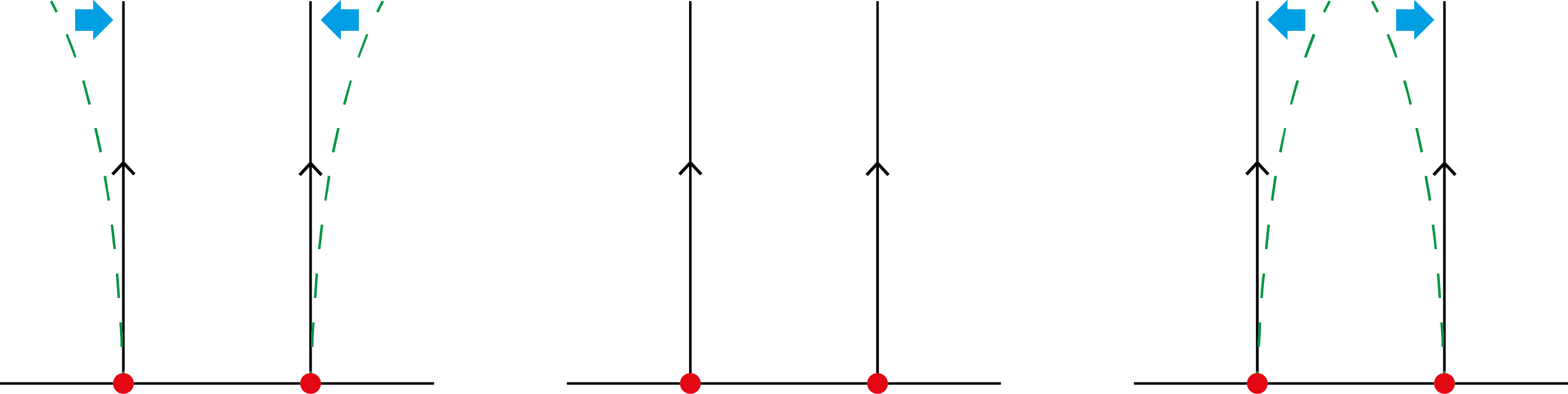
Figure 1.1: Sketch of re in the attracting-repelling family. The potential force, indicated with thick arrows, balances the tendency of the particles to defocus/focus for negative/positive curvature.

For $\kappa<0$ these motions correspond to the ‘hyperbolic’ re considered before in [7, 12, 4]. On the other hand, for $\kappa>0$ the motion corresponds to the ‘acute’ repelling re whose existence is noticed in the first part of this paper (section 2).

Our analysis of this family, together with our observation that the repelling and attractive 2-body problems on the sphere are equivalent (Lemma 2.4), provides an explanation of the mechanism responsible for the existence of obtuse re, studied in [2, 4], for the attractive 2-body problem on the sphere.

The balance of the potential forces with curvature described above, and illustrated in Figure 1.1, is very delicate and as a result these re are unstable for any separation $q$ when $\kappa\leq 0$ and for small values of $q\sqrt{\kappa}$ if $\kappa>0$. For the specific potential $V_{\kappa}(q)=\kappa\cot_{\kappa}(q)$, the linear approximation of the 5-dimensional reduced dynamics at $\kappa=0$ turns out to be nilpotent, of rank 2 and satisfying $L^{2}=0$. As $\kappa$ varies away from $0$, one zero eigenvalue remains, while the other 4 split into a pair of real and a pair of purely imaginary eigenvalues (see Figure 5.2).

We finish the introduction by mentioning that the treatment of the $N$-body problem on spaces of constant curvature, with the curvature $\kappa$ as parameter was recently considered by Diacu and collaborators [8, 9, 10]. The emphasis of the works [9, 10] is on deriving a set of equations of motion for the problem that depend smoothly on $\kappa$. However, their approach seems unnecessarily complicated, and the results become straightforward using the approach we adopt in Sec. 3 below. For example, it becomes self-evident that the equations of motion continue from $\kappa>0$ through $\kappa=0$ to $\kappa<0$. Moreover, in contrast to these references, our approach is naturally adapted to analysing changes in the curvature while keeping the distance between the masses fixed, which is essential to understanding the behaviour of the solutions as a function of $\kappa$.

2   Relative equilibria for repelling particles

Consider two particles, of masses $\mu_{1},\mu_{2}$, on the unit sphere $S$ in $\mathbb{R}^{3}$ interacting via a potential energy $V(q)$, where $q$ is the geodesic distance between the particles. We assume the interaction is repelling, which is equivalent to $V^{\prime}(q)<0$.

The configuration space is $Q=S\times S\subset\mathbb{R}^{3}\times\mathbb{R}^{3}$. Given $(\mathbf{x}_{1},\mathbf{x}_{2})\in Q$, the distance $q$ between them is the unique value $q\in[0,\pi]$ satisfying $\cos q=\mathbf{x}_{1}\cdot\mathbf{x}_{2}$.

Since the potential depends only on the distance $q$, the system is symmetric under the group of rigid rotations of the sphere, that is, under $\mathbf{SO}(3)$. Relative equilibria are those motions corresponding to 1-parameter subgroups of $\mathbf{SO}(3)$, which are all rotations at some speed around a fixed axis. We now state two theorems on the classification and stability of the relative equilibria for the repelling 2-body problem. The first is for the system with distinct masses, while the second is the analogous statement for equal masses. In every case, the two masses lie on the same side of the axis of rotation, as shown in Figures 2.1 and 2.2.

(a) Attracting potential

(b) Repelling potential

Figure 2.1: Isosceles and right-angled re for identical masses for the two types of potential—all rotating about the vertical axis

Theorem 2.1 (Equal masses).

If the two particles are of equal mass, there are two classes of re, isosceles and right-angled (see Fig. 2.1) as follows:

1. Given any $q\in(0,\pi)$, $q\neq\pi/2$, there is a unique re where the masses are separated by an angle $q$. In this case the axis of rotation is perpendicular to the sphere radius that passes midway between the masses; these we call isosceles re.

2. Given any $\theta\in(0,\pi/4]$ there is a unique re with angular separation $q=\pi/2$, called a right-angled re, where $\theta$ is the smaller of the angles between the axis of rotation and the masses.

Note that when $q=\pi/2$ and $\theta=\pi/4$ these two families meet in a pitchfork bifurcation, giving just one re. The angular velocities of the re are given by (2.2) below.

For the specific repelling potential $V(q)=\cot q$, the linear stability of the re is as follows. The isosceles re subtending an acute angle $q\in(0,\pi/2)$ are all unstable, while those subtending an obtuse angle $q\in(\pi/2,\pi)$ are elliptic. All right-angled re with $\theta\neq\pi/4$ are elliptic.

(a) Attracting potential

(b) Repelling potential

Figure 2.2: Acute and obtuse re for distinct masses for the two types of potential—both rotating about the vertical axis. The configurations shown are solutions for the mass ratio $\mu_{1}=0.75\,\mu_{2}$; they have $q=\pi/3$ or $2\pi/3$ for the acute and obtuse configurations respectively. The configurations on the right are obtained from those on the left by applying the antipodal map $\mathcal{A}$.

Theorem 2.2 (Distinct masses).

If the masses are distinct there are also two classes of re, acute and obtuse, as follows, see Figure 2.2.

For each $q\in(0,\pi)$, $q\neq\pi/2$, there is a unique re where the masses are separated by an angle $q$. The axis of rotation subtends angles $\theta_{j}\in(0,\pi/2)$ with the mass $\mu_{j}$ such that $q=\pi-(\theta_{1}+\theta_{2})$ (see Figure 2.2(b)) which are related by

$$\mu_{1}\sin(2\theta_{1})=\mu_{2}\sin(2\theta_{2}).$$ (2.1)

We call these acute and obtuse re, accordingly as $q<\pi/2$ or $q>\pi/2$. There is no re for $q=\pi/2$. In the acute re, the smaller mass is closer to the axis of rotation, while in the obtuse re, the larger mass is closer. See Fig. 2.2(b).

The angular velocity of the re is given by (2.2) below.

For the repelling potential given by $V(q)=\cot q$, the linear stability of these re are as follows. The obtuse re are all elliptic, while for the acute ones there is a critical angle $q^{\dagger}\in(0,\pi/2)$ (defined below), which depends on the mass ratio, for which acute re are linearly unstable for $0<q<q^{\dagger}$ and elliptic for $q^{\dagger}<q<\pi/2$.

In the setting of both theorems, the speed of rotation $\omega$ for all re is given by

$$\omega^{2}=\zeta^{-1}V^{\prime}(q),$$ (2.2)

where $\zeta=\frac{1}{2}\mu_{1}\sin(2\theta_{1})=\frac{1}{2}\mu_{2}\sin(2\theta_{2})$ and $q=\pi-(\theta_{1}+\theta_{2})$. The critical angle $q^{\dagger}$ satisfies

$$q^{\dagger}=\alpha^{\dagger}-\frac{\pi}{2}-\frac{1}{2}\sin^{-1}(\mu\sin 2\alpha^{\dagger})$$ (2.3)

where $\mu=\mu_{1}/\mu_{2}$ and $\alpha^{\dagger}$ is the unique solution in $(\pi/2,\pi)$ of the equation

$$\cos 2\alpha=2\sin^{2}\alpha\sqrt{1+\mu^{2}\sin^{2}2\alpha}.$$ (2.4)

We show how this follows from the results of [4] in the proof below.

As with the problem for attracting particles treated in [4], the Hamiltonian function cannot be used as a Lyapunov function to guarantee the nonlinear stability of the elliptic re of the problem. This is due to the non-definiteness of the Hamiltonian at these points. For the particular repelling potential given by $V(q)=\cot(q)$, we find the following.

Proposition 2.3.

The restriction to the symplectic leaf of the Hessian matrix of the reduced Hamiltonian, with $V(q)=\cot(q)$, at the re of the problem described in the theorems above, has the following signature:

$\mu_{1}=\mu_{2}$ :

1. Right-angled re which are not isosceles have signature $(++--)$.

2. Isosceles re subtending an acute angle have signature $(+++-)$.

3. Isosceles re subtending an obtuse angle have signature $(++--)$.

$\mu_{1}\neq\mu_{2}$ :

1. Acute re with $0<q<q^{\dagger}$ have signature $(+++-)$.

2. Acute re with $q^{\dagger}<q<\pi/2$ have signature $(++--)$.

3. Obtuse re  have signature $(++--)$.

In the equal mass case, one can clearly see from the change in signature of the Hamiltonian, the pitchfork bifurcation occuring as momentum is increased. The central family is the isosceles re with the right-angled re bifurcating off that family at $\theta=\pi/4$. (If we use $q$ as a parameter, then the pitchfork bifurcation is a ‘vertical bifurcation’ since the right-angled re all have $q=\pi/2$.)

In the case of distinct masses, the change in signature of the Hamiltonian at $q=q_{*}$ occurs at a saddle-node bifurcation where the angular momentum is minimal.

The theorem is a direct consequence of the results of [4] via the following observation.

Lemma 2.4.

Define the diffeomorphism $\mathcal{A}:Q\to Q$ by $\mathcal{A}(\mathbf{x}_{1},\mathbf{x}_{2})=(\mathbf{x}_{1},-\mathbf{x}_{2})$; that is, $\mathbf{x}_{2}$ is mapped to its antipodal point. This map transforms a repelling 2 body system on the sphere to an attracting one. Specifically, if the Lagrangian of the repelling system is

$$\mathcal{L}_{1}=\tfrac{1}{2}\mu_{1}\|\dot{\mathbf{x}}_{1}\|^{2}+\tfrac{1}{2}\mu_{2}\|\dot{\mathbf{x}}_{2}\|^{2}-V(q)$$

then the transformed system has

$$\mathcal{L}_{2}=\tfrac{1}{2}\mu_{1}\|\dot{\mathbf{x}}_{1}\|^{2}+\tfrac{1}{2}\mu_{2}\|\dot{\mathbf{x}}_{2}\|^{2}-V(\pi-q).$$

Note that if the first system is repelling, so $V^{\prime}(q)>0$, then the second is attracting: $\frac{\mathrm{d}}{\mathrm{d}q}V(\pi-q)<0$.

Proof:  Let $\mathcal{L}_{1}$ be as in the statement of the lemma. If $(\mathbf{x}_{1},\mathbf{x}_{2})$ are separated by distance $q$ then $\mathcal{A}(\mathbf{x}_{1},\mathbf{x}_{2})$ are separated by a distance of $q^{\prime}=\pi-q$. It follows that applying the map $\mathcal{A}$, or rather its lift $T\mathcal{A}$ to the tangent bundle, gives

$$\mathcal{L}\circ T\mathcal{A}=\tfrac{1}{2}\mu_{1}\|\dot{\mathbf{x}}_{1}\|^{2}+\tfrac{1}{2}\mu_{2}\|\dot{\mathbf{x}}_{2}\|^{2}-V(q^{\prime}).$$

Now $V(q^{\prime})=V(\pi-q)$ is a smooth increasing function of $q$, meaning that the transformed Lagrangian describes an attracting system. $\Box$

Proof: (of both theorems and the proposition) Consider the repelling system on $Q$ with potential $V$, a smooth decreasing function of $q\in(0,\pi)$. The Lagrangian is given by

$$\mathcal{L}=\tfrac{1}{2}\mu_{1}\|\dot{\mathbf{x}}_{1}\|^{2}+\tfrac{1}{2}\mu_{2}\|\dot{\mathbf{x}}_{2}\|^{2}-V(q).$$

By the lemma, the diffeomorphism $\mathcal{A}$ transforms the system with a repelling potential to one with an attracting potential. This new attracting system is precisely the subject of [4], and the two theorems above follow from Theorems 4.1 and 4.3 of that paper, after exchanging acute with obtuse (while right-angled configurations map to right-angled configurations, preserving $\theta$). For example, in [4, Theorem 4.3] it is shown that for different masses, the acute re are linearly stable. By applying the map $\mathcal{A}$, one deduces that the obtuse re for the repelling problem are linearly stable. The proposition follows similarly from [4, Proposition 4.4], after noting that $\cot(\pi-q)=-\cot(q)$.

The expression for the bifurcation value $q^{\dagger}$ requires more explanation. In [4, Sec. 4] the angle $\alpha$ is introduced as the angle between mass 1 and the axis of rotation, measured in the direction towards mass 2. It is found that the relation with $q$ is

$$\mu_{1}\sin(2\alpha)=\mu_{2}\sin(2(q-\alpha)).$$ (2.5)

This is a purely kinematic relation and is independent of any potential. For the specific potential $V=-\cot q$, it is shown in [4, Theorem 4.3] that the loss of stability occurs when $\alpha$ lies in the interval $(0,\pi/2)$ and satisfies (2.4); this value is denoted $\alpha^{*}$. The bifurcation then occurs when $q=q^{*}\in(\pi/2,\,\pi)$ satisfies (2.5).

Figure 2.3: The definition of $\alpha$ for the attracting system (left) and the resulting repelling configuration (right). The dashed line is the axis of rotation.

Given the same definition of $\alpha$, when applying the antipodal map $\mathcal{A}$, the angle $\alpha$ is changed to $\pi-\alpha$, as illustrated in Figure 2.3. Such $\alpha$ satisfies the same equation (2.4), but is now the solution in the interval $(\pi/2,\pi)$; call this value $\alpha^{\dagger}$ (equal to $\pi-\alpha^{*}$). In the attracting problem, $\alpha<q$ while in the repelling problem, $\alpha>q$ (as illustrated in the figure). If $q^{*}>\pi/2$ is the bifurcation value determined in [4] (for obtuse attracting configurations), then the corresponding bifurcation for the (acute) repelling problem is $q^{\dagger}=\pi-q^{*}$. It follows that $q^{\dagger}$ indeed satisfies (2.3). $\Box$

Remark 2.5.

It is usual to assume that $\lim_{q\to 0}V(q)$ and $\lim_{q\to\pi}V(q)$ are infinite, in which case the diagonal ($\mathbf{x}_{1}=\mathbf{x}_{2}$) and antipodal ($\mathbf{x}_{1}=-\mathbf{x}_{2}$) configurations are forbidden. In that case the re we have described above are all the possible ones. On the other hand, without this assumption (for example $V(q)=\pm\cos q$ where ‘$+$’ is repelling, ‘$-$’ is attracting), the diagonal and antipodal configurations will be equilibria, and motion around a great circle at any (common) speed will be a relative equilibrium. In the repelling case, the antipodal re and equilibria will be nonlinearly stable relative to the group of symmetries, while the diagonal ones will be unstable. For the attracting case, the existence is the same, but the stabilities are reversed. Some details in this direction can be found in [2].

As explained in the introduction, the mechanism responsible for the existence of the re in Theorems 2.1 and 2.2 that subtend an acute angle $q$ is the balance of the repelling forces with the tendency of the geodesics on the sphere to focus. The interpretation of the re that subtend an obtuse angle is more subtle as it involves the balance of centrifugal and attracting forces of $\mu_{1}$ and the ‘phantom attracting particle’ antipodal to $\mu_{2}$ in Lemma 2.4.

3   Curvature family

Combining the results of Section 2 with previous work on attracting potentials on surfaces of constant curvature, it is interesting to study how the families of relative equilibria are related as the curvature $\kappa$ varies from positive, through zero to negative values. Similar studies were done previously for the Kepler problem in [5] and for point vortices in [14], and we borrow freely from the approach taken in the latter paper.

Denote by $\mathcal{S}_{\kappa}$ the surface in $\mathbb{R}^{3}$ defined by

$$f_{\kappa}(x,y,z)=x^{2}+y^{2}+\kappa z^{2}-2z=0,$$ (3.1)

and on this surface we consider the restriction of the ambient metric in $\mathbb{R}^{3}$ given by

$$\mathrm{d}s^{2}=\mathrm{d}x^{2}+\mathrm{d}y^{2}+\kappa\,\mathrm{d}z^{2}.$$ (3.2)

Writing $K_{\kappa}=\mathrm{diag}[1,1,\kappa]$ for the metric tensor, we define the related norm by,

$$\|\mathbf{x}\|_{\kappa}^{2}=\mathbf{x}^{T}K_{\kappa}\mathbf{x},\quad\text{for }\mathbf{x}\in\mathbb{R}^{3}.$$

The Riemannian surface $\mathcal{S}_{\kappa}$ with the given metric is a surface of constant curvature $\kappa$, seen as follows. The equation (3.1) can also be written $x^{2}+y^{2}+\kappa(z-\frac{1}{\kappa})^{2}=\frac{1}{\kappa}$.

$\kappa>0$: Put $u=\sqrt{\kappa}(z-\frac{1}{\kappa})$; the metric becomes the usual Euclidean metric and the equation that of the sphere centred at the origin and of radius $1/\sqrt{\kappa}$, which is indeed of curvature $\kappa$. In the original coordinates, the centre is at $(x,y,z)=(0,0,1/\kappa)$. Note for future reference that for $\kappa>0$ the maximum distance between two points on $\mathcal{S}_{\kappa}$ is $\pi/\sqrt{\kappa}$.

$\kappa=0$: The metric on $\mathbb{R}^{3}$ is degenerate. However, restricted to the surface $\mathcal{S}_{0}$, which in this case is a paraboloid, it becomes a Riemannian metric, and moreover the orthogonal projection to the $x$-$y$ plane with the Euclidean metric is an isometry, showing that the metric on $\mathcal{S}_{0}$ has curvature zero.

$\kappa<0$: Here put $u=\sqrt{-\kappa}(z-\frac{1}{\kappa})$, to see that the metric is the standard Minkowski metric and the surface $\mathcal{S}_{\kappa}$ is a hyperboloid of 2 sheets. We restrict attention to the upper sheet, with $z\geq 0$, and it is then standard that this surface inherits a hyperbolic metric of constant curvature $\kappa$.

Remark 3.1.

For $\kappa\neq 0$, putting $(x,y,z)=(X/\sqrt{|\kappa|},\,Y/\sqrt{|\kappa|},\,Z/\kappa)$ maps $(x,y,z)\in\mathcal{S}_{\kappa}$ to $(X,Y,Z)\in\mathcal{S}_{\pm 1}$, and changes the metric to $\frac{1}{|\kappa|}K_{\pm 1}$. If the potential energy scales with $\kappa$ in a power law (as is the case for the potentials we consider below, viz. $V_{\kappa}(q)=-\cot_{\kappa}(q)$ and $\kappa\cot_{\kappa}(q)$) then, possibly after a rescaling of time depending on the power law, the Lagrangian scales and the systems for $\kappa=\kappa_{0}\neq 0$ and $\kappa=\mathrm{sign}(\kappa_{0})=\pm 1$ are equivalent.

3.1   Symmetry group

When $K_{\kappa}$ is invertible, the Lie group of linear transformations preserving the metric (3.2) is denoted $\mathbf{SO}(K_{\kappa})$. The elements $g$ satisfy $g^{T}K_{\kappa}g=K_{\kappa}$. For the Lie algebra, we have $\xi\in\mathfrak{so}(K_{\kappa})$ if and only if $\xi^{T}K_{\kappa}+K_{\kappa}\xi=0$. A basis for $\mathfrak{so}(K_{\kappa})$ is given by,

$$\xi_{1}=\begin{pmatrix}0&0&0\cr 0&0&-\kappa\cr 0&1&0\end{pmatrix},\quad\xi_{2}=\begin{pmatrix}0&0&\kappa\cr 0&0&0\cr-1&0&0\end{pmatrix},\quad\xi_{3}=\begin{pmatrix}0&-1&0\cr 1&0&0\cr 0&0&0\end{pmatrix}.$$ (3.3)

This basis satisfies the commutation relations

$$[\xi_{1},\,\xi_{2}]=\kappa\xi_{3},\quad[\xi_{2},\,\xi_{3}]=\xi_{1},\quad[\xi_{3},\,\xi_{1}]=\xi_{2}.$$

When $\kappa=0$, one sees that $g\in\mathbf{GL}(3)$ satisfies $g^{T}K_{0}g=K_{0}$ if and only if $g$ is of the form

$$g=\left(\begin{array}[]{c|c}A&\begin{matrix}0\cr 0\end{matrix}\cr\hline\cr\begin{matrix}a&b\end{matrix}&c\end{array}\right)$$ (3.4)

where $A\in\mathbf{O}(2)$, and $a,b,c\in\mathbb{R}$ with $c\neq 0$. This is a 4-dimensional group, whereas we need the subgroup isomorphic to $\mathbf{SE}(2)$ (as $\kappa=0$ corresponds to the Euclidean plane), and this is the subgroup with $c=1$. The Lie algebra of this subgroup coincides with the algebra generated by the $\xi_{j}$ above with $\kappa=0$. With this definition of $\mathbf{SO}(K_{0})$, from now on, we abbreviate $G_{\kappa}=\mathbf{SO}(K_{\kappa})$ and $\mathfrak{g}_{\kappa}=\mathfrak{so}(K_{\kappa})$.

The Lie algebra $\mathfrak{g}_{\kappa}$ is isomorphic to $\mathfrak{so}(3)$ for $\kappa>0$, to $\mathfrak{se}(2)$ for $\kappa=0$, and to $\mathfrak{sl}(2)\simeq\mathfrak{so}(2,1)$ for $\kappa<0$. Indeed, for $\kappa\neq 0$, the standard commutation relations are recovered by rescaling the basis to $\{|\kappa|^{-1/2}\xi_{1},\,|\kappa|^{-1/2}\xi_{2},\,\xi_{3}\}$. So

$$G_{\kappa}\simeq\begin{cases}\mathbf{SO}(3)&\text{if }\kappa>0\cr\mathbf{SE}(2)&\text{if }\kappa=0\cr\mathbf{SO}(2,1)&\text{if }\kappa<0.\end{cases}$$

Affine action

The linear action of $G_{\kappa}$ on $\mathbb{R}^{3}$ preserves the metric $K_{\kappa}$ (by construction). In order to preserve the surface $\mathcal{S}_{\kappa}$, the action needs to be modified by a translation $T_{\kappa}(g)$ depending on $g\in G_{\kappa}$ as follows:

$$g\cdot\mathbf{x}=g\mathbf{x}+T_{\kappa}(g),$$

where

$$T_{\kappa}(g)=\begin{cases}\frac{1}{\kappa}(I-g)\mathbf{e}_{3}&\text{if }\kappa\neq 0,\\[6.0pt] \begin{pmatrix}A\mathbf{u}\cr\frac{1}{2}|\mathbf{u}|^{2}\end{pmatrix}&\text{if }\kappa=0.\end{cases}$$

Here ${\mathbf{e}}_{3}=(0,0,1)^{T}$, and, for $\kappa=0$, $g$ is as in (3.4), with $c=1$ and we write $\mathbf{u}=(a,b)^{T}$. One can show that $T_{\kappa}(g_{\kappa})$ is continuous in $\kappa$, whenever $g_{\kappa}$ is a continuous family of matrices with $g_{\kappa}\in G_{\kappa}$.

The corresponding affine action of the Lie algebra $\mathfrak{g}_{\kappa}$ on $\mathbb{R}^{3}$ is given by

$$\xi\cdot\mathbf{x}=\xi\mathbf{x}+\tau(\xi),$$ (3.5)

where $\xi\mathbf{x}$ is the linear part (matrix times vector) and

$$\tau(\omega_{1}\xi_{1}+\omega_{2}\xi_{2}+\omega_{3}\xi_{3})=\begin{pmatrix}-\omega_{2}\cr\omega_{1}\cr 0\end{pmatrix}$$ (3.6)

is the translation.

Lie Poisson structure on $\mathfrak{g}_{\kappa}^{*}$

Throughout we will write $\mathbf{m}=(m_{1},m_{2},m_{3})$ for a point in $\mathfrak{g}_{\kappa}^{*}$ using the basis dual to the basis $\{\xi_{j}\}$. It is seen from the commutation relations that the minus Lie Poisson structure on $\mathfrak{g}_{\kappa}^{*}$ is determined by

$$\{m_{1},m_{2}\}=-\kappa m_{3},\quad\{m_{2},m_{3}\}=-m_{1},\quad\{m_{3},m_{1}\}=-m_{2}.$$

Hence, the bracket of functions $f,g$ on $\mathfrak{g}_{\kappa}^{*}$ is

$$\{f,\,g\}(\mathbf{m})=-\left(K_{\kappa}\mathbf{m},\nabla f\times\nabla g\right),$$ (3.7)

where $\times$ is the ordinary vector product in $\mathbb{R}^{3}$, and this holds also in the degenerate case $\kappa=0$. It follows immediately from the above formula that the function

$$C(\mathbf{m})=m_{1}^{2}+m_{2}^{2}+\kappa m_{3}^{2}$$ (3.8)

is a Casimir function of the bracket.

3.2   Equations of motion

There exist well-known functions that interpolate between the circular trigonometric functions and the hyperbolic ones. These are often denoted $\sin_{\kappa}$ and $\cos_{\kappa}$ (or $S_{\kappa}$ and $C_{\kappa}$) for $\kappa\in\mathbb{R}$ and are defined as follows,

$$\begin{array}[]{rcl}\sin_{\kappa}(x)&=&\begin{cases}\frac{1}{\sqrt{\kappa}}\,\sin(\sqrt{\kappa}\,x)&\text{if \ }\kappa>0,\cr x&\text{if \ }\kappa=0,\cr\frac{1}{\sqrt{-\kappa}}\,\sinh(\sqrt{-\kappa}\,x)&\text{if \ }\kappa<0,\cr\end{cases}\\[24.0pt] \cos_{\kappa}(x)&=&\begin{cases}\cos(\sqrt{\kappa}\,x)&\text{if \ }\kappa>0,\cr 1&\text{if \ }\kappa=0,\cr\cosh(\sqrt{-\kappa}\,x)&\text{if \ }\kappa<0,\cr\end{cases}\end{array}$$ (3.9)

Note that these are analytic functions of $(\kappa,x)$; indeed the Taylor series at the orgin are

$$\sin_{\kappa}(x)=x-\tfrac{1}{3!}\kappa x^{3}+\tfrac{1}{5!}\kappa^{2}x^{5}+\cdots,\qquad\cos_{\kappa}(x)=1-\tfrac{1}{2}\kappa x^{2}+\tfrac{1}{4!}\kappa^{2}x^{4}+\cdots.$$ (3.10)

It is easy to check that these functions satisfy similar relations to the usual trigonometric functions, for example $\cos_{\kappa}(x)^{2}+\kappa\sin_{\kappa}(x)^{2}=1$, and

$$\sin_{\kappa}(x+y) =\cos_{\kappa}(x)\sin_{\kappa}(y)+\sin_{\kappa}(x)\cos_{\kappa}(y),$$

$$\cos_{\kappa}(x+y) =\cos_{\kappa}(x)\cos_{\kappa}(y)-\kappa\sin_{\kappa}(x)\sin_{\kappa}(y).$$

Moreover, the derivatives satisfy $\sin_{\kappa}^{\prime}=\cos_{\kappa}$, and $\cos_{\kappa}^{\prime}=-\kappa\sin_{\kappa}$. In our application of these functions, $\kappa$ represents the Gauss curvature, and $x$ is replaced by $q$; note that $q$ has a unit of length, but $\sqrt{\kappa}$ has a unit of inverse-length, so the arguments of $\sin$, $\sinh$ etc., are dimensionless. See [5] for a similar use of these functions in the curved Kepler problem. One also defines other functions, such as $\tan_{\kappa}=\sin_{\kappa}/\cos_{\kappa}$ and $\cot_{\kappa}$ similarly.

Now consider 2 point masses on the surface $\mathcal{S}_{\kappa}$ of constant curvature $\kappa$. We assume the points are distinct, and when $\kappa>0$ that the points are not antipodal. The configuration space of this system is therefore

$$Q_{\kappa}=\mathcal{S}_{\kappa}\times\mathcal{S}_{\kappa}\setminus\Delta,$$

where $\Delta$ consists of the points on the diagonal (for all $\kappa$) together with pairs of antipodal points if $\kappa>0$.

The analysis that follows is very close to that in [4], so we omit the details of the calculations.

We parametrize points on $Q_{\kappa}$ as $Q_{\kappa}\simeq I_{\kappa}\times G_{\kappa}$, where $I_{\kappa}$ is the interval of allowed distances between the pair of points in a configuration. That is,

$$I_{\kappa}=\begin{cases}(0,\infty)&\text{if }\kappa\leq 0\cr(0,\pi/\sqrt{\kappa})&\text{if }\kappa>0.\end{cases}$$

Now, given $q\in I_{\kappa}$ consider the two points in $\mathbb{R}^{3}$,

$$\mathbf{x}_{1}=\begin{pmatrix}0\cr 0\cr 0\end{pmatrix},\qquad\mathbf{x}_{2}=\mathbf{x}_{2}(q)=\begin{pmatrix}0\cr\sin_{\kappa}(q)\cr\frac{1}{\kappa}(1-\cos_{\kappa}(q))\end{pmatrix}.$$

For $\kappa=0$ the final component of the point $\mathbf{x}_{2}$ is defined by continuity, giving $\frac{1}{2}q^{2}$, as can be seen from (3.10).

Lemma 3.2.

The points $\mathbf{x}_{1},\mathbf{x}_{2}$ lie in $\mathcal{S}_{\kappa}$ separated by a (geodesic) distance $q$.

Proof:  It is easy to check that both points lie in $\mathcal{S}_{\kappa}$. For $t\in[0,q]$ let

$$\gamma(t)=\begin{pmatrix}0\cr\sin_{\kappa}(t)\cr\frac{1}{\kappa}(1-\cos_{\kappa}(t))\end{pmatrix}.$$

Then $\gamma(0)=\mathbf{x}_{1}$, $\gamma(q)=\mathbf{x}_{2}$ and $\gamma(t)\in\mathcal{S}_{\kappa}$. A short calculation shows that $\|\dot{\gamma}(t)\|_{\kappa}^{2}=1$, whence $\gamma$ is a curve parametrized by arc length and the distance along $\gamma$ from the origin to $\mathbf{x}_{2}$ is therefore equal to $q$. There remains to argue that $\gamma$ is a geodesic. This follows by symmetry: the surface $\mathcal{S}_{\kappa}$ is a surface of revolution and $\gamma$ lies on a meridian. $\Box$

The parametrization (diffeomorphism) of $Q_{\kappa}$ by $I_{\kappa}\times G_{\kappa}$ is given by

$$(q,\,g)\longmapsto(g\cdot\mathbf{x}_{1},\,g\cdot\mathbf{x}_{2}(q))\in Q_{\kappa}.$$

Here $g\cdot\mathbf{x}$ is the affine action of $G_{\kappa}$ described above. To write down the Lagrangian we pass to the tangent bundles, and we use the left trivialization for $TG_{\kappa}=G_{\kappa}\times\mathfrak{g}_{\kappa}$, $(g,\dot{g})\mapsto(g,\xi)=(g,g^{-1}\dot{g})$. This gives

$$T\,I_{\kappa}\times TG_{\kappa} \longrightarrow TQ_{\kappa}\subset T\mathcal{S}_{\kappa}\times T\mathcal{S}_{\kappa}\subset\mathbb{R}^{6}\times\mathbb{R}^{6}$$

$$(q,\dot{q},g,\xi) \longmapsto (g\cdot\mathbf{x}_{1},\,g\xi\cdot\mathbf{x}_{1},\,g\cdot\mathbf{x}_{2},\,g\xi\cdot\mathbf{x}_{2}+g\mathbf{x}_{2}^{\prime}\dot{q}),$$

where $\mathbf{x}_{2}^{\prime}=(\frac{\mathrm{d}}{\mathrm{d}q}\mathbf{x}_{2})$. The fact we are using the left-trivialization of $TG$ means that $\xi$ is to be interpreted as angular velocity in the body frame [13].

Now consider a general motion. Associated to $(q(t),g(t))$ in $I_{\kappa}\times G$, write

$$\mathbf{X}_{1}(t)=g(t)\cdot\mathbf{x}_{1},\quad\text{and}\quad\mathbf{X}_{2}(t)=g(t)\cdot\mathbf{x}_{2}(q(t)).$$

Given a potential $V_{\kappa}(q)$, the Lagrangian $\mathcal{L}:TQ_{\kappa}\to\mathbb{R}$ is then given in terms of this parametrization as follows,

$$\mathcal{L} = \tfrac{1}{2}\mu_{1}\|\dot{\mathbf{X}}_{1}\|_{\kappa}^{2}+\tfrac{1}{2}\mu_{2}\|\dot{\mathbf{X}}_{2}\|_{\kappa}^{2}-V_{\kappa}(q)$$

$$= \tfrac{1}{2}\mu_{1}\|g(\xi\cdot\mathbf{x}_{1})\|_{\kappa}^{2}+\tfrac{1}{2}\mu_{2}\|g(\xi\cdot\mathbf{x}_{2}+\mathbf{x}_{2}^{\prime}\dot{q})\|_{\kappa}^{2}-V_{\kappa}(q)$$

$$= \tfrac{1}{2}\mu_{1}\|\xi\cdot\mathbf{x}_{1}\|_{\kappa}^{2}+\tfrac{1}{2}\mu_{2}\|\xi\cdot\mathbf{x}_{2}+\mathbf{x}_{2}^{\prime}\dot{q}\|_{\kappa}^{2}-V_{\kappa}(q)$$

$$= \tfrac{1}{2}\mu_{1}\|\tau(\xi)\|_{\kappa}^{2}+\tfrac{1}{2}\mu_{2}\|\xi\mathbf{x}_{2}+\tau(\xi)+\mathbf{x}_{2}^{\prime}\dot{q}\|_{\kappa}^{2}-V_{\kappa}(q).$$

Here we have used the fact that $g$ is norm-preserving. Writing,

$$\xi=\omega_{1}\xi_{1}+\omega_{2}\xi_{2}+\omega_{3}\xi_{3},$$

by (3.6), we obtain $\|\tau(\xi)\|_{\kappa}^{2}=(\omega_{1}^{2}+\omega_{2}^{2})$ and a short calculation shows that,

$$\xi\mathbf{x}_{2}+\tau(\xi)+\mathbf{x}_{2}^{\prime}\dot{q}=\begin{pmatrix}-\sin_{\kappa}(q)\,\omega_{3}-\cos_{\kappa}(q)\,\omega_{2}\cr\cos_{\kappa}(q)(\omega_{1}+\dot{q})\cr\sin_{\kappa}(q)(\omega_{1}+\dot{q})\end{pmatrix}$$

whence

$$\|\xi\mathbf{x}_{2}+\tau(\xi)+\mathbf{x}_{2}^{\prime}\dot{q}\|_{\kappa}^{2}=(\omega_{1}+\dot{q})^{2}+(\sin_{\kappa}(q)\omega_{3}+\cos_{\kappa}(q)\omega_{2})^{2}.$$

Combining these expressions, one obtains

$$\mathcal{L}=\tfrac{1}{2}\mathbf{v}^{T}\mathbb{M}\mathbf{v}-V_{\kappa}(q),$$

where $\mathbf{v}=(\dot{q},\omega_{1},\omega_{2},\omega_{3})$, and the mass matrix $\mathbb{M}$ is given by

$$\mathbb{M}=\begin{pmatrix}\mu_{2}&\mu_{2}&0&0\cr\mu_{2}&\mu_{1}+\mu_{2}&0&0\cr 0&0&\mu_{1}+\mu_{2}C^{2}&\mu_{2}SC\cr 0&0&\mu_{2}SC&\mu_{2}S^{2}\end{pmatrix}.$$ (3.11)

Here and in the matrix below, $S=\sin_{\kappa}(q)$ and $C=\cos_{\kappa}(q)$. Recall that when $\kappa=0$ then $C=1$ and $S=q$.

To pass to the Hamiltonian formulation, we use the Legendre transform, with $p=\partial\mathcal{L}/\partial\dot{q}$, and $m_{j}=\partial\mathcal{L}/\partial\omega_{j}$ ($j=1,2,3$). This involves the left trivialization of $T^{*}G_{\kappa}$ as $G_{\kappa}\times\mathfrak{g}_{\kappa}^{*}$ (see for example [13]). Putting $\mathbf{u}=(p,m_{1},m_{2},m_{3})$, one finds.

$$H=\tfrac{1}{2}\mathbf{u}^{T}\mathbb{M}^{-1}\mathbf{u}+V_{\kappa}(q),$$ (3.12)

with

$$\mathbb{M}^{-1}=\frac{1}{\mu_{1}\mu_{2}}\begin{pmatrix}\mu_{1}+\mu_{2}&-\mu_{2}&0&0\cr-\mu_{2}&\mu_{2}&0&0\cr 0&0&\mu_{2}&-\tfrac{\mu_{2}C}{S}\cr 0&0&-\tfrac{\mu_{2}C}{S}&\tfrac{1}{S^{2}}(\mu_{1}+\mu_{2}C^{2})\end{pmatrix}.$$ (3.13)

Reduction

The Hamiltonian $H(q,p,g,\mathbf{m})$ is independent of $g\in G_{\kappa}$, so induces a smooth function on the smooth Poisson reduced space $P=T^{*}I_{\kappa}\times\mathfrak{g}_{\kappa}^{*}$, which we also denote $H=H(q,p,\mathbf{m})$. The reduced equations of motion are determined by the Poisson structure arising from the left trivialization [13],

$$\{q,p\}=1,\quad\{m_{1},m_{2}\}=-\kappa m_{3},\quad\{m_{2},m_{3}\}=-m_{1},\quad\{m_{3},m_{1}\}=-m_{2}\,;$$

brackets between other coordinates being zero. The equations of motion of the reduced system are therefore,

$$\dot{q}=H_{p},\quad\dot{p}=-H_{q},\quad\text{and}\quad\dot{\mathbf{m}}=(K_{\kappa}\mathbf{m})\times(H_{\mathbf{m}}).$$ (3.14)

Both the Hamiltonian and the Casimir $C$ given by (3.8) are first integrals.

3.2.1   Flat case: $\kappa=0$

The usual approach to the 2-body problem in the plane is to fix the centre of mass (at the origin), which implies vanishing total momentum $\mathbf{p}=0$, and to use the relative vector $\mathbf{r}=\mathbf{x}_{2}-\mathbf{x}_{1}$ for configuration space, which then satisfies a central force law (the Kepler problem). However, that approach does not fit into the family with non-zero curvature, since these problems have no preferred centre of mass frame. We therefore describe briefly the relation between the usual ‘central force’ approach and the one we need to take here.

Let

$$\mathbf{p}_{1}=\mu_{1}\dot{\mathbf{x}}_{1},\qquad\mathbf{p}_{2}=\mu_{2}\dot{\mathbf{x}}_{2},\qquad\mathbf{p}=\mathbf{p}_{1}+\mathbf{p}_{2},$$

be the usual momenta and $\mathbf{r}=\mathbf{x}_{2}-\mathbf{x}_{1}$. The variables $(q,p,m_{1},m_{2},m_{3})$ then correspond to

$$q=\|\mathbf{r}\|,\quad p=\frac{\mathbf{r}\cdot\mathbf{p}_{2}}{q},\quad m_{1}=\frac{\mathbf{r}\cdot\mathbf{p}}{q},\quad m_{2}=\frac{\mathbf{r}\times\mathbf{p}}{q},\quad m_{3}=\mathbf{r}\times\mathbf{p}_{2},$$ (3.15)

where $\mathbf{r}\times\mathbf{p}$ denotes the scalar quantity given by the third component of the cross product of the vectors $(\mathbf{r},0),(\mathbf{p},0)\in\mathbb{R}^{3}$ (and similarly for $\mathbf{r}\times\mathbf{p}_{2}$). In particular, the angular momentum about the centre of mass is given by

$$L=m_{3}-\frac{\mu_{2}\,q}{\mu_{1}+\mu_{2}}m_{2},$$ (3.16)

which is a first integral of the equations of motion (3.14) in this case where $\kappa=0$, and in this case the Casimir is $C=m_{1}^{2}+m_{2}^{2}=\|\mathbf{p}\|^{2}$.

Remark 3.3.

Given that $L$ is an integral, it is natural to ask what the corresponding Hamiltonian flow (or group action) is. In fact this is simply planar rotations of the plane about the centre of mass. Its expression in terms of the variables $(q,p,m_{1},m_{2},m_{3})$ can be determined from (3.15). In particular $(m_{1},m_{2})$ rotates about the origin, thus preserving the Casimir $C=m_{1}^{2}+m_{2}^{2}=\|\mathbf{p}\|^{2}$.

3.3   Relative equilibria

Relative equilibria are equilibrium points of the reduced system so they correspond to solutions of the following equations (see (3.14)):

$$\frac{\partial H}{\partial p} =0,$$ (3.17a)

$${K_{\kappa}\mathbf{m}}\times\frac{\partial H}{\partial\mathbf{m}} ={\bf 0},$$ (3.17b)

$$\frac{\partial H}{\partial q} =0.$$ (3.17c)

Equations (3.17a) and (3.17b) are the kinematic equations (independent of the potential), while (3.17c) is the dynamical equation. We assume throughout that $V_{\kappa}^{\prime}(q)\neq 0$ for all $q$ (except in one case when $\kappa=0$ —see the end of this section and Section 5).

These equations were analysed in [4] for $\kappa\neq 0$, but we outline the calculations again here, following a different approach that is more convenient for our purposes. First fix $q\in I_{\kappa}$. Combining equations (3.17a) and (3.17c) shows that

$$m_{1}=\frac{\mu_{1}+\mu_{2}}{\mu_{2}}\,p,\quad\text{and}\quad p\bigl{(}\mu_{2}\sin_{\kappa}(q)m_{2}-(\mu_{1}+\mu_{2})\cos_{\kappa}(q)m_{3}\bigr{)}=0.$$

Hence either $p=m_{1}=0$ or there are linear relations between $m_{2}$ and $m_{3}$, and between $p$ and $m_{1}$.

If $p\neq 0$ then the remaining equations lead to $V^{\prime}(q)=0$, which we are assuming is not satisfied.

Now assume $p=m_{1}=0$, which implies that (3.17a) and the second and third components of (3.17b) hold. The dynamical equation (3.17c) is equivalent to

$$m_{2}=\frac{(\mu_{1}+\mu_{2})\cos_{\kappa}(q)m_{3}^{2}-\sin_{\kappa}^{3}(q)V_{\kappa}^{\prime}(q)}{\mu_{2}\sin_{\kappa}(q)m_{3}}.$$ (3.18)

Using this, one may eliminate $m_{2}$ from the first component of (3.17b) and obtain a biquadratic equation for $m_{3}$,

$$am_{3}^{4}+bm_{3}^{2}+c=0$$

whose coefficients $a,b$ and $c$ depend on $q,\kappa$ and the masses. Denote by $\mu$ the mass ratio $\mu=\mu_{1}/\mu_{2}$, and for the rest of the paper we assume, without any loss of generality, that $0<\mu\leq 1$ and $\mu_{2}=1$.

The solution of this biquadratic equation leads to the following conditions for re:

1.

If either $\kappa<0$ or $\kappa>0$ and $q\neq\pi/(2\sqrt{\kappa})$ then $m_{3}^{2}=A_{\pm}(q,\kappa,\mu)$ where:

$$A_{\pm}(q,\kappa,\mu)=-\frac{\left(2\mu\cos_{\kappa}^{2}(q)+1-\mu\pm\sqrt{4\mu\cos_{\kappa}^{2}(q)+(\mu-1)^{2}}\right)\sin_{\kappa}(q)V_{\kappa}^{\prime}(q)}{2\mu\kappa\cos_{\kappa}(q)}.$$ (3.19)

2.

If $\kappa>0$ and $q={\pi}/{2\sqrt{\kappa}}$, then $a=b=0$ and we obtain the condition

$$(\mu-1)V_{\kappa}^{\prime}(q)=0$$ (3.20)

which is independent of $m_{3}$ and only has solutions if the masses are equal.

3.

If $\kappa=0$ then $a=0$, and we are left with a linear equation whose unique solution is

$$m_{3}^{2}=\frac{\mu q^{3}}{1+\mu}V_{0}^{\prime}(q).$$ (3.21)

In case 3 above, the value of $m_{3}^{2}$ is the limiting value of $A_{-}$ as $\kappa\to 0$. In case 1 we have $m_{3}^{2}=A_{\pm}(q,\kappa,\mu)$ so there are relative equilibria provided that $A_{\pm}(q,\kappa,\mu)$ is positive. The following lemma gives necessary and sufficient conditions for this. Recall that $q\sqrt{\kappa}$ is a dimensionless quantity.

Lemma 3.4.

For any value of $\mu\in(0,1]$, the quantity $A_{\pm}(q,\kappa,\mu)$ defined by (3.19) has the following properties:

Suppose the potential is attractive, $V_{\kappa}^{\prime}(q)>0$, then:

if $\kappa<0$ then $A_{\pm}(q,\kappa,\mu)$ is positive for all $q>0$;

if $\kappa>0$ then $A_{-}(q,\kappa,\mu)$ is positive if and only if $q<\pi/2\sqrt{\kappa}$, and $A_{+}(q,\kappa,\mu)$ is positive if and only if $\pi/2<q\sqrt{\kappa}<\pi$.

Suppose, on the other hand, the potential is repelling, $V_{\kappa}^{\prime}(q)<0$, then

if $\kappa<0$ then $A_{\pm}(q,\kappa,\mu)$ is negative for all $q>0$;

if $\kappa>0$ then $A_{+}(q,\kappa,\mu)$ is positive if and only if $q\sqrt{\kappa}<\pi/2$, and $A_{-}(q,\kappa,\mu)$ is positive if and only if $\pi/2<q\sqrt{\kappa}<\pi$.

The proof is postponed to the end of the section. We now state two propositions classifying the relative equilibria for attracting and repelling potentials. Our labelling of the re  uses the terminology of [4]. In our classification we do not distinguish re  related by the time reversibility of the problem.

Proposition 3.5 (Classification of relative equilibria for an attractive potential).

In the presence of an attractive potential $V_{\kappa}^{\prime}(q)>0$, the classification of relative equilibria of the problem is as indicated below.

If $\kappa<0$ then for any $q>0$ there are exactly two relative equilibria respectively having

$$\begin{split}m_{3}^{2}&=A_{+}(q,\kappa,\mu)\qquad\mbox{({hyperbolic {re}})},\\ m_{3}^{2}&=A_{-}(q,\kappa,\mu)\qquad\mbox{({elliptic {re}}).}\end{split}$$

For both relative equilibria $p=m_{1}=0$ and $m_{2}$ is determined by (3.18).

If $\kappa>0$ then for any $0<q<\pi/\sqrt{\kappa}$, $q\neq\pi/2\sqrt{\kappa}$, there is exactly one relative equilibrium having

$$\begin{split}m_{3}^{2}&=A_{+}(q,\kappa,\mu)\quad\mbox{if $\quad\pi/2<q\sqrt{\kappa}<\pi$}\quad\mbox{({obtuse attractive {re}})},\\ m_{3}^{2}&=A_{-}(q,\kappa,\mu)\quad\mbox{if $\quad 0<q\sqrt{\kappa}<\pi/2$}\quad\mbox{({acute attractive {re}})},\end{split}$$

In both cases $p=m_{1}=0$ and $m_{2}$ is determined by (3.18).

If $\kappa>0$ and $q\sqrt{\kappa}=\pi/2$, then a relative equilibrium is possible only if the two masses are equal. In this case there is a family of relative equilibria parametrized by $m_{3}$ having $p=m_{1}=0$ and $m_{2}$ given by (3.18). These are right-angle attractive re.

If $\kappa=0$ then for any $q>0$ there is exactly one relative equilibrium determined by

$$m_{3}^{2}=\frac{\mu q^{3}}{1+\mu}V_{0}^{\prime}(q),\qquad m_{2}=m_{1}=p=0.$$

These are the usual Keplerian re: two bodies rotating uniformly about their centre of mass.

Proof:  The proof follows from Equations (3.19), (3.20), (3.21) and Lemma 3.4. $\Box$

The classification for a repelling potential (similar to the result of Section 2) is given by the following.

Proposition 3.6 (Classification of relative equilibria for a repelling potential).

In the presence of a repelling potential $V_{\kappa}^{\prime}(q)<0$, the classification of relative equilibria of the problem is as follows.

If $\kappa\leq 0$ there are no relative equilibria.

If $\kappa>0$ then for any $q$ satisfying $0<q<\pi/\sqrt{\kappa}$, $q\neq\pi/(2\sqrt{\kappa})$, there is exactly one relative equilibrium having

$$\begin{split}m_{3}^{2}&=A_{-}(q,\kappa,\mu)\quad\mbox{if $\quad\pi/2<q\sqrt{\kappa}<\pi$}\quad\mbox{({obtuse repelling {re}})},\\ m_{3}^{2}&=A_{+}(q,\kappa,\mu)\quad\mbox{if $\quad 0<q\sqrt{\kappa}<\pi/2$}\quad\mbox{({acute repelling {re}})},\end{split}$$

In both cases $p=m_{1}=0$ and $m_{2}$ is determined by (3.18).

If $\kappa>0$ and $\sqrt{\kappa}\,q=\pi/2$, then a relative equilibrium is possible only if the two masses are equal. In this case there is a family of relative equilibria parametrized by $m_{3}$ having $p=m_{1}=0$ and $m_{2}$ given by (3.18). These are right-angled repelling re.

Note that our classification results in the repelling case for $\kappa>0$ may be recovered from the results for the attractive case together with Lemma 2.4.

We finish the section with a proof of Lemma 3.4.

Proof:  (of Lemma 3.4) We only treat the attractive case where $V_{\kappa}^{\prime}(q)>0$, the other is analogous.

It is clear that the numerator of $A_{+}(q,\kappa,\mu)$ is positive, so its sign is given by the denominator. For $\kappa<0$ we have $\cos_{\kappa}(q)>0$ for all $q>0$. On the other hand, for $\kappa>0$, we have $\cos_{\kappa}(q)>0$ for $0<q\sqrt{\kappa}<\pi/2$ and $\cos_{\kappa}(q)<0$ for $\pi/2<q\sqrt{\kappa}<\pi$, and the conclusions follow from these considerations.

To analyse the sign of $A_{-}(q,\kappa,\mu)$ we start from the identity

$$\left(4\mu\cos_{\kappa}^{2}(q)+(\mu-1)^{2}\right)-\left(2\mu\cos_{\kappa}^{2}(q)+1-\mu\right)^{2}=4\kappa\mu^{2}\cos_{\kappa}^{2}(q)\sin_{\kappa}^{2}(q).$$

From this equation it is straightforward to obtain

$$\mbox{sign}\left(2\mu\cos_{\kappa}^{2}(q)+1-\mu-\sqrt{4\mu\cos_{\kappa}^{2}(q)+(\mu-1)^{2}}\right)=-\mbox{sign}(\kappa),$$

and the conclusions about the sign of $A_{-}(q,\kappa,\mu)$ follows from the above considerations about the sign of $\cos_{\kappa}(q)$. $\Box$

Remark 3.7.

Extending Proposition 3.8 above, if, for arbitrary $\kappa$, and some particular value $q_{0}$ of $q$, the potential satisfies $V_{\kappa}^{\prime}(q_{0})=0$ then it follows from (3.18) that re  occur with

$$p=\frac{m_{1}}{1+\mu},\qquad m_{2}=(\mu+1)\,\cot_{\kappa}(q_{0})\,m_{3}.$$

Such motion corresponds to the two particles lying at a distance where the force vanishes, and following respective geodesics with equal speeds maintaining this constant separation. For $\kappa=0$, this amounts to the particles having equal velocity.

3.3.1   Flat case: $\kappa=0$

Again it is useful to discuss how the the results above relate to the well-known properties of the 2-body problem in the plane. First if the interaction is repelling, Proposition 3.6 tells us there are no relative equilibria, as is to be expected: indeed there are no motions where the particles remain at a constant distance.

More interesting is the case of an attracting potential; see Proposition 3.5. The Keplerian re consist of uniform rotations about a fixed centre of mass. However, notice that there are motions where the particles remain at a constant distance that are not relative equilibria: namely, those motions where the particles rotate uniformly about the centre of mass, but the centre of mass is uniformly translating relative to the (fixed) plane. These become re if one includes Galilean ssymmetry, but since such symmetries do not extend to the curved surfaces it is not helpful in this analysis.

Finally, for the purposes of section 5, we consider the motion with vanishing potential. In the absence of any interaction, the two particles will perform independent rectilinear motion. These are re precisely when they have identical velocities; up to Euclidean symmetry, there is a two parameter family of such motions, classified in terms of the reduced variables in the following proposition, whose proof follows immediately from the analysis of (3.17) with the simplifications $\sin_{0}(q)=q$, $\cos_{0}(q)=1$ and $V_{0}^{\prime}(q)=0$.

Proposition 3.8 (Classification of relative equilibria in the absence of interaction for $\kappa=0$).

In the absence of potential $V$, and for $\kappa=0$ and any $q>0$ and $0<\mu\leq 1$ there is a two-parameter family of re  of the problem determined by the conditions

$$p=\frac{m_{1}}{1+\mu},\qquad m_{2}=\frac{\mu+1}{q}\,m_{3}.$$ (3.22)

Following (3.15), the first relation signifies $\dot{q}=0$, while the second is equivalent to vanishing angular momentum about the centre of mass ($L=0$ in (3.16)). We are especially interested in the special class of re  having $p=m_{1}=0$: those where the velocities are perpendicular to the line joining the particles as these turn out to be the re arising as limits of re  with $\kappa\neq 0$, the so-called ‘perpendicular re’ in the introduction and in Section 5 below.

4   Attracting family

We consider here the family of re  that extend the Keplerian re in the plane. The interaction potential $V_{\kappa}$ is assumed to be always attractive and to depend smoothly on $\kappa$. This is related to the work [5] concerning the variation of the Kepler problem as the curvature is varied through 0.

4.1   The family of relative equilibria

Suppose $V_{\kappa}(q)$ is a smooth family of functions (i.e., smooth in both $q$ and $\kappa$) defined for $q\in I_{\kappa}$, and such that for each $\kappa$, $V_{\kappa}$ is an increasing function of $q$. The canonical example would be the graviational potential

$$V_{\kappa}(q)=-G\cot_{\kappa}(q)$$

where the constant $G>0$ encodes the gravitational constant and the masses. Since $V_{\kappa}^{\prime}(q)>0$, the terminology and relevant conclusions of the previous section come from Proposition 3.5.

Theorem 4.1.

Let $V_{\kappa}(q)$ be a smooth family of attractive potentials i.e. $V_{\kappa}^{\prime}(q)>0$ for all $q$ and $\kappa$. Fix $0<\mu\leq 1$ and $q>0$, and consider $\kappa\in(-\infty,(\pi/2q)^{2})$. Then, for the given values of $q$ and $\mu$, there is a smooth transition from the elliptic re for $\kappa<0$ to the acute attractive re  for $\kappa>0$. These re  are interpolated at $\kappa=0$ by the Keplerian re .

Proof:  The re  under consideration have $m_{3}^{2}=A_{-}(q,\kappa,\mu)$ if $\kappa\neq 0$ and $m_{3}^{2}=\frac{\mu q^{3}}{1+\mu}V_{0}^{\prime}(q)$ if $\kappa=0$. For all of them $m_{2}$ is given by (3.18) and $p=m_{1}=0$.

The smooth dependence of these re  away from $\kappa=0$ is clear from the expression for $A_{-}(q,\kappa,\mu)$ in (3.19). In particular, for $\kappa\neq 0$, the denominator does not vanish by our assumption that $\kappa<(\pi/2q)^{2}$. The behaviour of $A_{-}(q,\kappa,\mu)$ in the vicinity of $\kappa=0$ is analysed using the series expansions (3.10). We obtain

$$A_{-}(q,\kappa,\mu)=\frac{\mu q^{3}}{1+\mu}V_{\kappa}^{\prime}(q)-\frac{\mu q^{5}}{(1+\mu)^{3}}V_{\kappa}^{\prime}(q)\kappa+\mathcal{O}(\kappa^{2})\qquad\mbox{as}\quad\kappa\to 0.$$

This proves that $A_{-}(q,\kappa,\mu)$ can be extended smoothly to $\kappa=0$ and moreover that such extension satisfies

$$A_{-}(q,0,\mu)=\frac{\mu q^{3}}{1+\mu}V_{0}^{\prime}(q),$$

which is the value of $m_{3}^{2}$ for the Keplerian re . The proof is completed by noting that (3.18) depends smoothly on $\kappa$. $\Box$

Figure 4.1 illustrates how the re  in the family of the theorem vary as the value of the curvature passes from positive to negative.

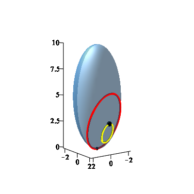
(a) $\kappa=0.2$

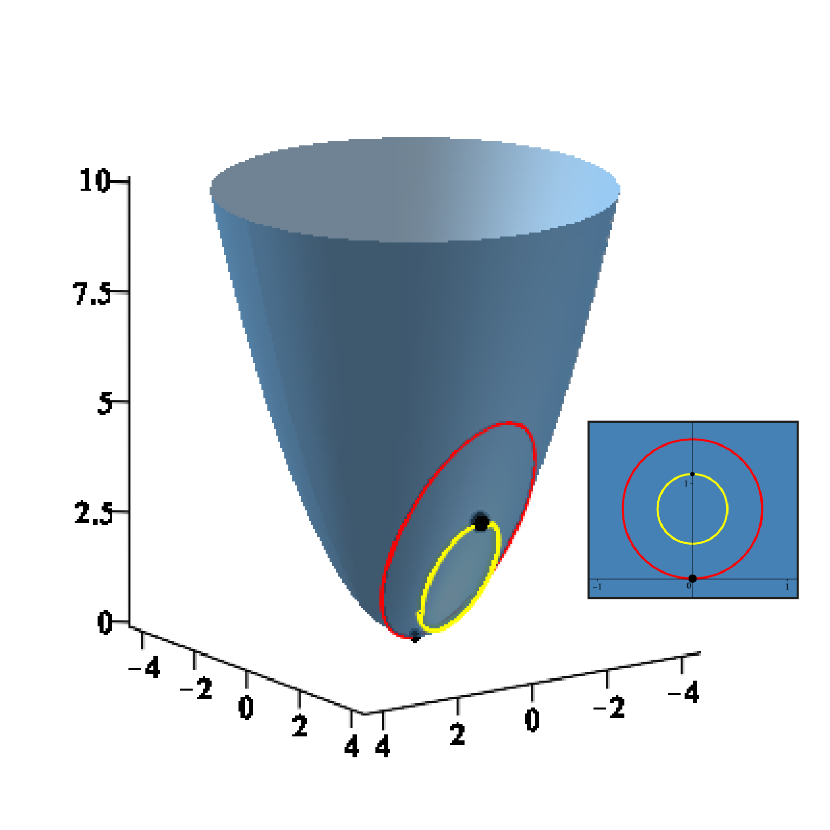
(b) $\kappa=0$

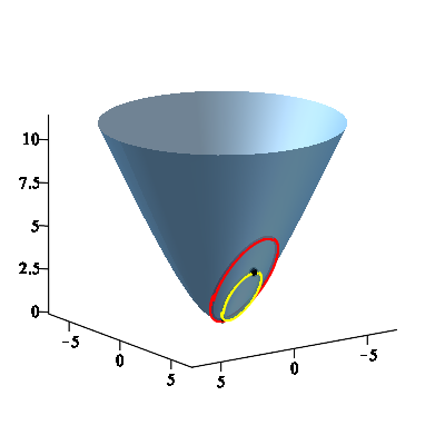
(c) $\kappa=-0.2$

Figure 4.1: Family of re  of Theorem 4.1 for the potential $V_{\kappa}(q)=-\cot_{\kappa}(q)$ with $\mu=0.5$ and $q=2.5$. For $\kappa=0$, the inset figure shows the orthogonal projection of the trajectories onto the plane which are concentric circles.

We finish the section by noting that the value of the Casimir function $C$ given by (3.8) has the following asymptotic expansion along the re  considered in this section:

$$C=\frac{\mu q^{3}}{1+\mu}V_{\kappa}^{\prime}(q)\kappa+\mathcal{O}(\kappa^{2}),\qquad\mbox{as}\quad\kappa\to 0.$$ (4.1)

Therefore, in our convention, the sign of the Casimir coincides with the sign of the curvature along this family.

4.2   Linearization & stability

Now consider the potential $V_{\kappa}(q)=-\cot_{\kappa}(q)$, and in particular $V_{0}$ is the Newtonian potential $-1/q$.

The linearization of the reduced equations around the equilibrium having $q=q_{0}$, $p=m_{1}=0$, and

$$\begin{split}m_{3}=\sqrt{A_{-}(q_{0},\kappa,\mu)},\qquad m_{2}=\frac{\cos_{\kappa}(q_{0})(\mu+1)A_{-}(q_{0},\kappa,\mu)-\mu\sin_{\kappa}(q_{0})}{\sqrt{A_{-}(q,\kappa,\mu)}\sin_{\kappa}(q_{0})},\end{split}$$

has the form

$$\frac{\mathrm{d}}{\mathrm{d}t}{\bf w}=L(q_{0},\mu,\kappa){\bf w},\qquad{\bf w}=(q,p,m_{1},m_{2},m_{3})^{t},$$

where the $5\times 5$ matrix $L(q_{0},\mu,\kappa)$ has the following asymptotic expansion as $\kappa\to 0$:

$$L(q_{0},\mu,\kappa)=L_{0}(q_{0},\mu)+L_{1}(q_{0},\mu)\kappa+\mathcal{O}(\kappa^{2}).$$

Here

$$L_{0}(q_{0},\mu)=\begin{pmatrix}0&\frac{\mu+1}{\mu}&-\frac{1}{\mu}&0&0\\ \rule[-15.0pt]{0.0pt}{24.0pt}-\frac{1}{q_{0}^{3}}&0&0&-\frac{1}{q_{0}^{3/2}\sqrt{\mu(\mu+1)}}&\frac{2\sqrt{\mu+1}}{q_{0}^{5/2}\sqrt{\mu}}\\ 0&0&0&\frac{\sqrt{\mu+1}}{q_{0}^{3/2}\sqrt{\mu}}&0\\ \rule[-12.0pt]{0.0pt}{24.0pt}0&0&-\frac{\sqrt{\mu+1}}{q_{0}^{3/2}\sqrt{\mu}}&0&0\\ 0&0&-\frac{1}{q_{0}^{1/2}\sqrt{\mu(\mu+1)}}&0&0\end{pmatrix},$$

and

$$L_{1}(q_{0},\mu)=\begin{pmatrix}0&0&0&0&0\\ \rule[-12.0pt]{0.0pt}{24.0pt}\frac{-\mu(\mu+2)}{q_{0}(\mu+1)^{2}}&0&0&-\frac{\sqrt{\mu q_{0}}(\mu+2)}{2(\mu+1)^{5/2}}&\frac{\sqrt{\mu+1}}{3\sqrt{\mu q_{0}}}\\ \frac{1}{q_{0}(\mu+1)}&0&0&\frac{\sqrt{\mu q_{0}}(\mu-2)}{2(\mu+1)^{3/2}}&\frac{1}{\sqrt{\mu(\mu+1)q_{0}}}\\ \rule[-12.0pt]{0.0pt}{24.0pt}0&-\sqrt{\frac{q_{0}}{\mu(\mu+1)}}&-\sqrt{\frac{q_{0}}{\mu}}\left(\frac{\mu^{2}-2\mu-2}{2(\mu+1)^{3/2}}\right)&0&0\\ 0&-\frac{q_{0}^{3/2}}{(\mu+1)^{3/2}\sqrt{\mu}}&\frac{q_{0}^{3/2}(\mu^{2}+2\mu+4)}{6\sqrt{\mu}(\mu+1)^{5/2}}&0&0\end{pmatrix}.$$

The characteristic polynomial of $L(q_{0},\mu,\kappa)$ defined by

$$p(x)=\det(L(q_{0},\mu,\kappa)-x\mbox{Id}_{5})$$

may be written as

$$p(x)=-x\left(x^{2}+\frac{\mu+1}{\mu q_{0}^{3}}+\mathcal{O}(\kappa^{2})\right)\left(x^{2}+\frac{\mu+1}{\mu q_{0}^{3}}+\frac{2\kappa(\mu^{2}+1)}{(\mu+1)\mu q_{0}}+\mathcal{O}(\kappa^{2})\right).$$

For small values of $\kappa$ one sees that all the four non-zero eigenvalues are imaginary (and double when $\kappa=0$: we expect that to be a feature of the $1/r$ potential). See Figure 4.2.

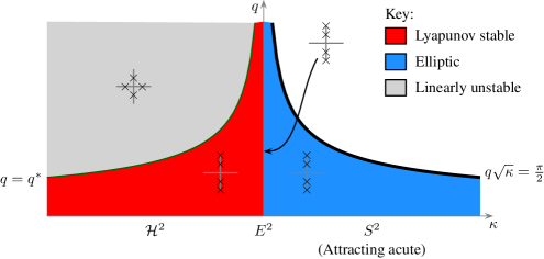
Figure 4.2: Stability and eigenvalue pattern for re of Kepler type in the attracting family with distinct masses, with $V_{\kappa}(q)=-\cot_{\kappa}(q)$. See Remark 4.2 for the definition of $q^{*}$.

The asymptotics of these eigenvalues as $\kappa\to 0$ are

$$\pm i\left(\sqrt{\frac{\mu+1}{\mu q_{0}^{3}}}+\mathcal{O}(\kappa^{2})\right),\quad\text{and}\quad\pm i\left(\sqrt{\frac{\mu+1}{\mu q_{0}^{3}}}+\sqrt{\frac{q_{0}}{(\mu+1)^{3}\mu}}(1+\mu^{2})\kappa+\mathcal{O}(\kappa^{2})\right).$$

The double eigenvalues therefore separate with bounded speed in $\kappa$, as $\kappa$ moves from 0.

We end this section by addressing the question of why the eigenvalues at $\kappa=0$ are double, by relating the motion to the known behaviour of the Kepler problem. Firstly, for $\kappa=0$, the re in question satisfies $p=m_{1}=m_{2}=0$, so is at a singular point of the Casimir, which for $\kappa=0$ is $C=m_{1}^{2}+m_{2}^{2}=\|\mathbf{p}\|^{2}$, see Sec. 3.2.1, and satisfies

$$m_{3}^{2}=\frac{\mu q}{1+\mu}.$$

Let $\widehat{\mathbf{x}}=(\widehat{q},\widehat{p},\widehat{m}_{1},\widehat{m}_{2},\widehat{m}_{3})$ be a tangent vector at the (relative) equilibrium in the Poisson reduced space $\mathbb{R}^{5}$. The kernel of $L_{0}(q_{0},\mu)$ is spanned by the vector $\widehat{\mathbf{x}}=(2\sqrt{q_{0}(\mu+1)},\,0,\,0,\,0,\,\sqrt{\mu})^{t}$, which is tangent to the curve of re. For the non-zero eigenvalues, consider first the effect of varying $(m_{1},m_{2})$ away from 0. In the original dynamics (on $\mathbb{R}^{4}$), this amounts to increasing the momentum $\mathbf{p}$. The resulting motion is a superposition of the Kepler rotation and a uniform translation of the centre of mass. In the reduced space, this is a periodic orbit, with period equal to the period of rotation of the Kepler solution.

On the other hand, if we remain on the subset $m_{1}=m_{2}=0$ (where the Casimir vanishes, which is therefore an invariant submanifold), the function $m_{3}$ coincides with the angular momentum $L$ and so is conserved. Putting $m_{3}=\ell$ (a constant) we have a reduced 1 degree of freedom system in $(q,p)$ which coincides with the usual reduction with amended potential,

$$V_{\mathrm{am}}(q)=V_{0}(q)+\frac{A}{q^{2}},$$

for some constant $A$ depending on $\mu$ and $\ell$. The small oscillations near the equilibrium of this reduced system consists of elliptical orbits in the original system, and these are periodic with the same period as the circular motion.

Thus all the periodic motions have the same period as the period of the circular Keplerian orbit represented by the re in question.

Remark 4.2.

While our primary interest in this paper involves the bifurcations arising as $\kappa$ passes through 0, Figures 4.2 and 5.2 show some other stability changes. These are specifically for the potential $V_{\kappa}(q)=-\cot_{\kappa}(q)$ and $V_{\kappa}(q)=\kappa\cot_{\kappa}(q)$ respectively, and follow respectively from [4] and Theorem 2.2, adapted using the rescaling of Remark 3.1. The transition between (linearly) stable and unstable re occurs respectively when $q=q^{*}$ and $q=q^{\dagger}$. For the potential $V_{\kappa}(q)=-\cot_{\kappa}(q)$ treated in this section, the transition occurs when $\kappa<0$ and $q^{*}$ satisfies

$$q^{*}=\alpha^{*}+\frac{1}{2}\sin_{\kappa}^{-1}(\mu\sin_{\kappa}2\alpha^{*}),$$ (4.2)

where $\alpha^{*}$ is the unique solution to the equation

$$\cos_{\kappa}2\alpha=2|\kappa|\sin_{\kappa}^{2}\alpha\sqrt{1-\kappa\mu^{2}\sin_{\kappa}^{2}2\alpha}.$$ (4.3)

On the other hand, in Section 5 below we consider $V_{\kappa}(q)=\kappa\cot_{\kappa}(q)$, and then the transition occurs when $\kappa>0$ and the interaction is repelling. In this case, the bifurcation will occur for the acute configuration at $q^{\dagger}$ given by the appropriate modification of (2.3),

$$q^{\dagger}=\alpha^{\dagger}-\frac{\pi}{2\sqrt{\kappa}}-\frac{1}{2}\sin_{\kappa}^{-1}(\mu\sin_{\kappa}2\alpha^{\dagger})$$

where $\alpha^{\dagger}\in[\pi/2\sqrt{\kappa},\,\pi/\sqrt{\kappa}]$ satisfies (4.3).

Remark 4.3.

Figure 4.2 shows that, for $\kappa<0$, the re of elliptic type are Lyapunov stable, but on the other hand for $\kappa>0$ they are merely elliptic. However, calculations in [4, Sec. 4.2] involving a KAM argument, show that for small values of $q\sqrt{\kappa}$ these are also Lyapunov stable (see also Fig. 11 there). For the intermediate value $\kappa=0$, the circular Kepler orbits are well-known to be Lyapunov stable relative to $\mathbf{SE}(2)$.

5   Attracting-repelling family

In this final section we consider the family of re  that extend the ‘perpendicular re’ defined in the introduction. We will assume that the interaction potential $V_{\kappa}(q)$ is repelling for $\kappa>0$, vanishes for $\kappa=0$ and is attracting for $\kappa<0$. Again, $V_{\kappa}$ should be defined for $q\in I_{\kappa}$. An example would be $V_{\kappa}(q)=\kappa\cot_{\kappa}(q)$.

5.1   The family of relative equilibria

The terminology and relevant conclusions for our analysis of the attracting-repelling family come from Propositions 3.5, 3.6 and 3.8. The following theorem shows that our assumption on the potential allows us to connect smoothly the hyperbolic re  for $\kappa<0$ with the acute repelling re  for $\kappa>0$.

Theorem 5.1.

Let $V_{\kappa}(q)=-\kappa U_{\kappa}(q)$ be a smooth family of potentials having $U_{\kappa}^{\prime}(q)>0$ for all $q$ and $\kappa$, so that the interaction between the particles is repelling for $\kappa>0$, vanishes for $\kappa=0$ and is attracting for $\kappa<0$.

Fix $0<\mu\leq 1$ and $q>0$, and consider $\kappa\in(-\infty,(\pi/2q)^{2})$. Then, for the given values of $q$ and $\mu$, there is a smooth transition from the hyperbolic re for $\kappa<0$ to the acute repelling re  for $\kappa>0$. These re  are interpolated at $\kappa=0$ by the re  of the planar 2-body problem with no interaction satisfying

$$m_{3}^{2}=\frac{(\mu+1)q}{\mu}\,U^{\prime}_{0}(q),\qquad m_{2}=\frac{\mu+1}{q}\,m_{3},\qquad p=m_{1}=0.$$

With no interaction, all solutions of the planar 2-body problem consist of the 2 particles in rectilinear motion. These are re (relative to the Euclidean group) precisely when their velocities are equal. In addition, it follows from (3.15) that the re satisfy the conditions in the theorem if their common velocity is perpendicular to the line joining the particles (called ‘perpendicular motion’ in the introduction).

Proof:  For $\kappa\neq 0$, the re  under consideration have $m_{3}^{2}=A_{+}(q,\kappa,\mu)$, $m_{2}$ given by (3.18) and $p=m_{1}=0$. The expression (3.18) may be evaluated at $\kappa=0$ and, under our assumption that $V_{0}^{\prime}(q)=0$, it simplifies to $m_{2}=\frac{\mu+1}{q}\,m_{3}$. Hence, to complete the proof we only need to show that $A_{+}(q,\kappa,\mu)$ admits a smooth extension at $\kappa=0$ and that this extension satisfies $A_{+}(q,0,\mu)=\frac{(\mu+1)q}{\mu}U^{\prime}_{0}(q)$. But this is obvious from (3.19) since our assumption on the form of $V_{\kappa}(q)$ cancels the factor of $\kappa$ in the denominator of $A_{+}(q,\kappa,\mu)$ and $A_{+}(q,0,\mu)$ may be directly evaluated to obtain the given value. $\Box$

Figure 5.1 illustrates how the re  of the family described in the theorem vary as the value of the curvature passes from positive to negative.

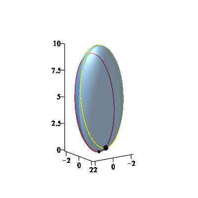
(a) $\kappa=0.2$ (repelling)

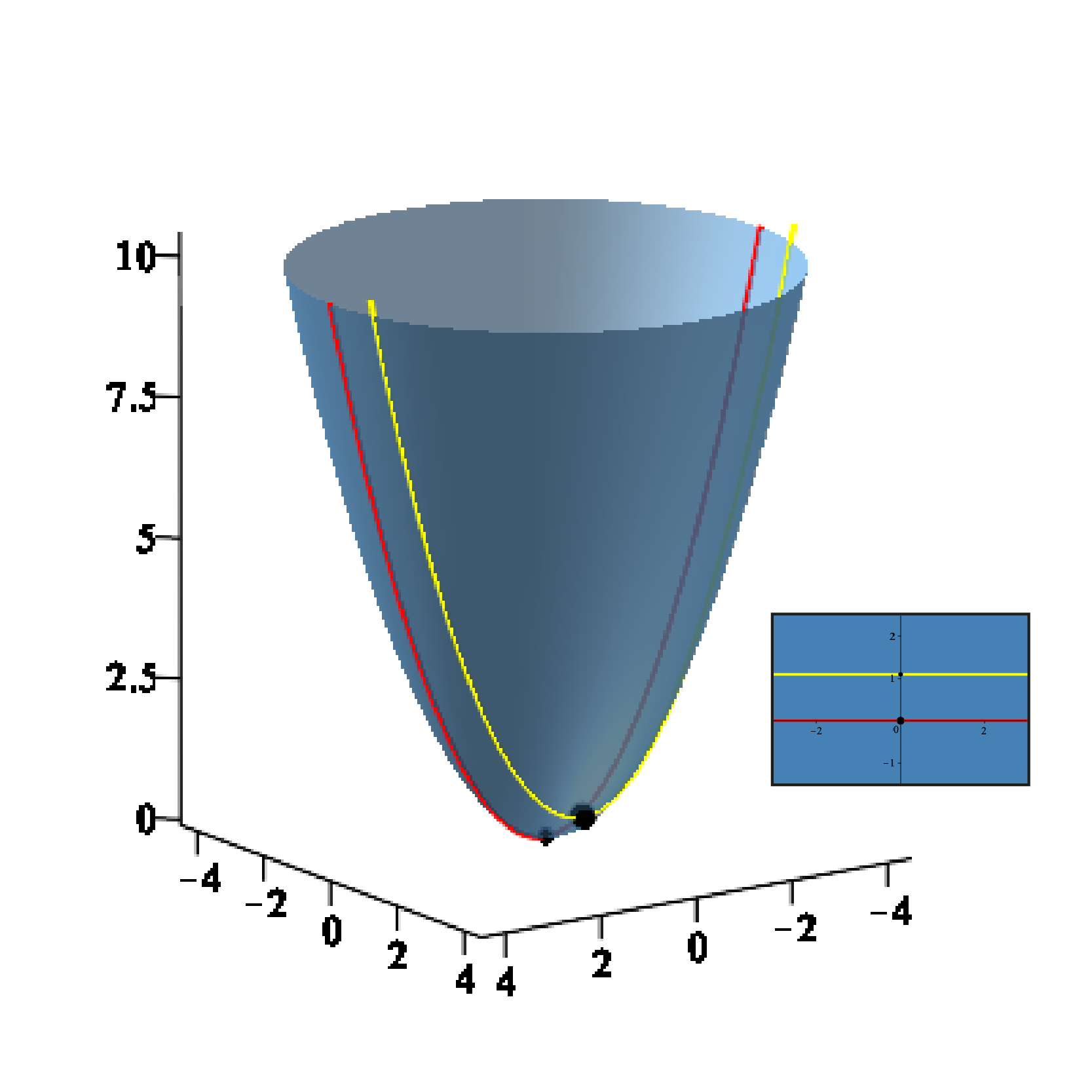
(b) $\kappa=0$ (no interaction)

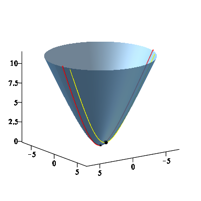
(c) $\kappa=-0.2$ (attracting)

Figure 5.1: Family of re  of Theorem 5.1 for the potential $V_{\kappa}(q)=\kappa\cot_{\kappa}(q)$ with $\mu=0.5$ and $q=1.1$. In the case of $\kappa=0$, the inset figure shows the orthogonal projection of the two curves to the plane which are parallel lines.

We end up by giving the asymptotic expansion around $\kappa=0$ for the Casimir function $C$ given by (3.8) along the family of re  considered in this section. Under the assumption that $V_{\kappa}=-\kappa U_{\kappa}(q)$ as in the statement of Theorem 5.1 we have

$$C=\left(\frac{(\mu+1)^{2}U_{\kappa}^{\prime}(q)}{\mu m_{3}}\right)^{2}+\mathcal{O}(\kappa)\qquad\mbox{as}\qquad\kappa\to 0.$$

Therefore the Casimir is positive for all members of this family.

Remark 5.2.

The theorem and proof are easily generalised to allow more general potentials transitioning the attractive interaction for $\kappa<0$ with the repelling interaction for $\kappa>0$. In particular, one may allow $V^{\prime}_{\kappa}(q)$ to vanish at higher order in $\kappa$ at $\kappa=0$ in which case one finds that the interpolating re  at $\kappa=0$ have $m_{3}=m_{2}=0$. Namely, in such case, the limiting re  at $\kappa=0$ become equilibria where the masses do not move (and $C=0$ when $\kappa=0$).

5.2   Linearization & stability

Assume $V_{\kappa}(q)=\kappa\cot_{\kappa}(q)$. The linearization of the reduced equations around the equilibrium at $q=q_{0}$, $p=m_{1}=0$ and

$$\quad m_{3}=\sqrt{A_{+}(q_{0},\kappa,\mu)}\,,\quad m_{2}=\frac{\cos_{\kappa}(q_{0})(\mu+1)A_{+}(q_{0},\kappa,\mu)+\kappa\mu\sin_{\kappa}(q_{0})}{\sqrt{A_{+}(q_{0},\kappa,\mu)}\sin_{\kappa}(q_{0})},$$

has the form

$$\frac{\mathrm{d}}{\mathrm{d}t}{\bf w}=L(q_{0},\mu,\kappa){\bf w},\qquad{\bf w}=(q,p,m_{1},m_{2},m_{3})^{t},$$

where the $5\times 5$ matrix $L(q_{0},\mu,\kappa)$ has the following asymptotic expansion as $\kappa\to 0$:

$$L(q_{0},\mu,\kappa)=L_{0}(q_{0},\mu)+L_{1}(q_{0},\mu)\kappa+L_{2}(q_{0},\mu)\kappa^{2}+\mathcal{O}(\kappa^{3}).$$

Here

$$L_{0}(q_{0},\mu)=\begin{pmatrix}0&\frac{\mu+1}{\mu}&-\frac{1}{\mu}&0&0\\ \rule[-14.0pt]{0.0pt}{24.0pt}-\frac{(\mu+1)^{2}}{\mu^{2}q_{0}^{5}}&0&0&-\frac{\sqrt{\mu+1}}{\mu^{3/2}q_{0}^{5/2}}&\frac{(\mu+1)^{3/2}}{\mu^{3/2}q_{0}^{7/2}}\\ \rule[-12.0pt]{0.0pt}{24.0pt}-\frac{(\mu+1)^{3}}{\mu^{2}q_{0}^{5}}&0&0&-\frac{(\mu+1)^{3/2}}{\mu^{3/2}q_{0}^{5/2}}&\frac{(\mu+1)^{5/2}}{\mu^{3/2}q_{0}^{7/2}}\\ 0&0&0&0&0\\ 0&\left(\frac{\mu+1}{\mu q_{0}}\right)^{3/2}&-\frac{\sqrt{\mu+1}}{(\mu q_{0})^{3/2}}&0&0\end{pmatrix}.$$

Explicit expressions for $L_{1}$ and $L_{2}$ can be found by lengthy computations.

The characteristic polynomial of $L(q_{0},\mu,\kappa)$ defined by

$$p(x)=\det(L(q_{0},\mu,\kappa)-x\mbox{Id}_{5})$$

may be written as

$$p(x)=-x\left(x^{4}+b(q_{0},\mu,\kappa)x^{2}+c(q_{0},\mu,\kappa)\right).$$

with

$$b(q_{0},\mu,\kappa)=\frac{2(\mu+1)}{\mu q_{0}^{3}}\kappa+\mathcal{O}(\kappa^{2}),\qquad c(q_{0},\mu,\kappa)=-\frac{3(\mu+1)^{2}\kappa^{2}}{\mu^{2}q_{0}^{6}}+\mathcal{O}(\kappa^{3}).$$

Note that $x=0$ is an eigenvalue of $L$ for all $\kappa$; this is due to the Casimir being an integral of motion. Indeed $L^{t}\,\nabla C=0$.

At $\kappa=0$, the all eigenvalues of the matrix $L_{0}$ vanish; indeed $L_{0}$ is nilpotent of rank 2 and index 2 ($L_{0}^{2}=0$—see below for an explanation). As $\kappa$ moves away from zero, and for fixed $q=q_{0}$, one finds asymptotic expansions as $\kappa\to 0$ for the 4 non-zero eigenvalues to be

$$\pm B_{0}\sqrt{\kappa}+\mathcal{O}(\kappa^{3/2})\quad\text{and}\quad\pm B_{0}\sqrt{-3\kappa}+\mathcal{O}(\kappa^{3/2}),$$

where $B_{0}^{2}=\frac{2(\mu+1)}{\mu q_{0}^{3}}$. We see that, regardless of the sign of $\kappa$, two of these are real and two are imaginary as illustrated in Figure 5.2. They move away from 0 with unbounded speed, as one sees in traditional saddle-node or pitchfork bifurcations.

Figure 5.2: Stability and eigenvalue pattern for re of translation type in the attracting-repelling family with $V_{\kappa}(q)=\kappa\cot_{\kappa}(q)$. (See Fig. 4.2 for the colour key and Remark 4.2 for the definition of $q^{\dagger}$.)

We describe briefly the geometry of the nilpotency of $L_{0}$. Fix $\kappa=0$, and consider the re that is perpendicular motion. The set of all equilibria of the reduced equations is 3-dimensional, parametrized for example by $(q,p,m_{3})$ and satisfying (3.22). The tangent space to this subspace accounts for the 3-dimensional kernel of $L_{0}$. Since $L_{0}$ is nilpotent of index 2, the image of $L_{0}$ lies in this subspace, and in particular coincides with the tangent space to the set of equilibria contained in the level set of the Casimir.

Acknowledgements

The authors acknowledge support of a Newton Advanced Fellowship from the Royal Society, Ref: NA140017 that financed the early stages of this research. LGN is thankful to the Alexander von Humboldt Foundation for a Georg Forster Advanced Research Fellowship that funded a research visit to TU Berlin where part of his contribution to this research was done, and also to Department of Mathematics of the University of Manchester for its hospitality during his visit in April 2019.

L.C. García-Naranjo
Departamento de Matemáticas y Mecánica IIMAS-UNAM
Apdo. Postal: 20-726 Mexico City, 01000, Mexico
luis@mym.iimas.unam.mx

J. Montaldi
Department of Mathematics, University of Manchester
Manchester M13 9PL, UK
j.montaldi@manchester.ac.uk

References

- [1] P. Arathoon, Singular reduction of the 2-body problem on the 3-sphere and the 4-dimensional spinning top. Preprint (2019). https://arxiv.org/abs/1904.00801
-
[2]
A.V. Borisov, I.S. Mamaev & A.A. Kilin,
Two-body problem on a sphere. Reduction, stochasticity, periodic orbits.
Regul. Chaotic Dyn. 9 (2004), 265–279.
https://doi.org/10.1070/RD2004v009n03ABEH000280 -
[3]
A.V. Borisov, I.S. Mamaev & I.S. Bizyaev, The spatial problem of 2 bodies on a sphere. Reduction and stochasticity. Regul. Chaotic Dyn. 21 (2016), 556–580.
https://doi.org/10.1134/S1560354716050075 - [4] A.V. Borisov, L.C. García-Naranjo, I.S. Mamaev & J. Montaldi, Reduction and relative equilibria for the two-body problem on spaces of constant curvature. Celest. Mech. Dyn. Astr. 130:43 (2018), 36pp. https://doi.org/10.1007/s10569-018-9835-7
- [5] J.F. Cariñena, M.F. Rañada & M. Santander, Central potentials on spaces of constant curvature: the Kepler problem on the two-dimensional sphere and the hyperbolic plane . J. Math. Phys. 46 (2005), 052702. https://doi.org/10.1063/1.1893214
-
[6]
F. Diacu, Relative Equilibria of the Curved N-Body Problem. Atlantis, Paris (2012).
https://doi.org/10.2991/978-94-91216-68-8 -
[7]
F. Diacu, E. Pérez-Chavela, & J.G. Reyes,
An intrinsic approach in the curved n-body problem. The negative case.
J. Differ. Equ. 252 (2012) 4529–4562.
https://doi.org/10.1016/j.jde.2012.01.002 - [8] F. Diacu, Bifurcations of the Lagrangian orbits from the classical to the curved 3-body problem. J. Math. Phys. 57 (2016), 112701, 20 pp. https://doi.org/10.1063/1.4967443
-
[9]
F. Diacu, S. Ibrahim, & J. Śniatycki,
The continuous transition of Hamiltonian vector fields through manifolds of constant curvature.
J. Math. Phys. 57 (2016), 062701, 9 pp.
https://doi.org/10.1063/1.4953371 - [10] F. Diacu, The classical N-body problem in the context of curved space. Canad. J. Math. 69 (2017), 790–806. https://doi.org/10.4153/CJM-2016-041-2
- [11] F. Diacu, C. Stoica, & S. Zhu, Central configurations of the curved N-body problem. J. Nonlinear Sci. 28 (2018), 1999–2046. https://doi.org/10.1007/s00332-018-9473-y
- [12] L.C. García-Naranjo, J.C. Marrero, E. Pérez-Chavela & M. Rodríguez-Olmos, Classification and stability of relative equilibria for the two-body problem in the hyperbolic space of dimension 2. J. Differ. Equ. 260 (2016), 6375–6404. https://doi.org/10.1016/j.jde.2015.12.044
- [13] J.E. Marsden & T.S. Ratiu, Introduction to Mechanics and Symmetry. Springer-Verlag, 1999. (2nd Ed.). https://doi.org/10.1007/978-0-387-21792-5
- [14] J. Montaldi & T. Tokieda, Deformation of geometry and bifurcations of vortex rings. Recent Trends in Dynamical Systems, pp. 335–370. Springer Proceedings in Mathematics & Statistics, vol 35. Springer, 2013. https://doi.org/10.1007/978-3-0348-0451-6_14