Magnon-phonon interactions in magnetic insulators

Abstract

We address the theory of magnon-phonon interactions and compute the corresponding quasi-particle and transport lifetimes in magnetic insulators with focus on yttrium iron garnet at intermediate temperatures from anisotropy- and exchange-mediated magnon-phonon interactions, the latter being derived from the volume dependence of the Curie temperature. We find in general weak effects of phonon scattering on magnon transport and the Gilbert damping of the macrospin Kittel mode. The magnon transport lifetime differs from the quasi-particle lifetime at shorter wavelengths.

I Introduction

Magnons are the elementary excitations of magnetic order, i.e. the quanta of spin waves. They are bosonic and carry spin angular momentum. Of particular interest are the magnon transport properties in yttrium iron garnet (YIG) due to its very low damping ($\alpha<10^{-4}$), which makes it one of the best materials to study spin-wave or spin caloritronic phenomena [1, 2, 3, 4, 5, 6]. For instance, the spin Seebeck effect (SSE) in YIG has been intensely studied in the past decade [7, 8, 9, 10, 11, 12, 13]. Here, a temperature gradient in the magnetic insulator injects a spin current into attached Pt contacts that is converted into a transverse voltage by the inverse spin Hall effect. Most theories explain the effect by thermally induced magnons and their transport to and through the interface to Pt [7, 14, 15, 16, 17, 18, 19]. However, phonons also play an important role in the SSE through their interactions with magnons [20, 21, 22].

Magnetoelastic effects in magnetic insulators were addressed first by Abrahams and Kittel [23, 24, 25], and by Kaganov and Tsukernik [26]. In the long-wavelength regime, the strain-induced magnetic anisotropy is the most important contribution to the magnetoelastic energy, whereas for shorter wavelengths, the contribution from the strain-dependence of the exchange interaction becomes significant [27, 28, 29]. Rückriegel et al. [28] computed very small magnon decay rates in thin YIG films due to magnon-phonon interactions with quasi-particle lifetimes $\tau_{qp}\apprge 480\;\mathrm{ns,}$even at room temperature. However, these authors do not consider the exchange interaction and the difference between quasi-particle and transport lifetimes.

Recently, it has been suggested that magnon spin transport in YIG at room temperature is driven by the magnon chemical potential [3, 30]. Cornelissen et al.  [3] assume that at room temperature magnon-phonon scattering of short-wavelength thermal magnons is dominated by the exchange interaction with a scattering time of $\tau_{qp}\sim 1\;\mathrm{ps}$, which is much faster than the anisotropy-mediated magnon-phonon coupling considered in Ref. [28] and efficiently thermalizes magnons and phonons to equal temperatures without magnon decay. Recently, the exchange-mediated magnon-phonon interaction [31] has been taken into account in a Boltzmann approach to the SSE, but this work underestimates the coupling strength by an order of magnitude, as we will argue below.

In this paper we present an analytical and numerical study of magnon-phonon interactions in bulk ferromagnetic insulators, where we take both the anisotropy- and the exchange-mediated magnon-phonon interactions into account. By using diagrammatic perturbation theory to calculate the magnon self-energy, we arrive at a wave-vector dependent expression of the magnon scattering rate, which is the inverse of the magnon quasi-particle lifetime $\tau_{qp}$. The magnetic Grüneisen parameter $\Gamma_{m}=\partial\ln T_{C}/\partial\ln V$ [32, 33], where $T_{C}$ is the Curie temperature and $V$ the volume of the magnet, gives direct access to the exchange-mediated magnon-phonon interaction parameter. We predict an enhancement in the phonon scattering of the Kittel mode at the touching points of the two-magnon energy (of the Kittel mode and a finite momentum magnon) and the longitudinal and transverse phonon dispersions, for YIG at around $1.3\;\mathrm{T}$ and $4.6\;\mathrm{T}$. We also emphasize the difference in magnon lifetimes that broaden light and neutron scattering experiments, and the transport lifetimes that govern magnon heat and spin transport.

The paper is organized as follows: in Sec. II we briefly review the theory of acoustic magnons and phonons in ferro-/ferrimagnets, particularly in YIG. In Sec. III we derive the exchange- and anisotropy-mediated magnon-phonon interactions for a cubic Heisenberg ferromagnet with nearest neighbor exchange interactions in the long-wavelength limit. In Sec. IV we derive the magnon decay rate from the imaginary part of the magnon self-energy in a diagrammatic approach and in Sec. V we explain the differences between the magnon quasi-particle and transport lifetimes. Our numerical results for YIG are discussed in Sec. VI. Finally in Sec. VII we summarize and discuss the main results of the present work. The validity of our long-wavelength approximation is analyzed in Appendix A and in Appendix B we explain why second order magnetoelastic couplings may be disregarded. In Appendix C we briefly discuss the numerical methods used to evaluate the k-space integrals.

II Magnons and phonons in ferromagnetic insulators

Without loss of generality, we focus our treatment on yttrium iron garnet (YIG). The magnon band structure of YIG has been determined by inelastic neutron scattering [34, 35, 36] and by ab initio calculation of the exchange constants [37]. The complete magnon spectral function has been computed for all temperatures by atomistic spin simulations [38], taking all magnon-magnon interactions into account, but not the magnon-phonon scattering. The pure phonon dispersion is known as well [39, 29]. In the following, we consider the interactions of the acoustic magnons from the lowest magnon band with transverse and longitudinal acoustic phonons, which allows a semi-analytic treatment but limits the validity of our results to temperatures below $100\;\mathrm{K}$. Since the low-temperature values of the magnetoelastic constants, sound velocities, and magnetic Grüneisen parameter are not available for YIG, we use throughout the material parameters under ambient conditions.

II.1 Magnons

Spins interact with each other via dipolar and exchange interactions. We disregard the former since at the energy scale $E_{\mathrm{dip}}\approx 0.02\;\mathrm{meV}$ [28] it is only relevant for long-wavelength magnons with wave vectors $k\lesssim 6\times 10^{7}\;\mathrm{m}^{-1}$ and energies $E_{\mathbf{k}}/k_{B}\lesssim 0.2\;\mathrm{K}$, which are negligible for the thermal magnon transport in the temperature regime we are interested in. The lowest magnon band can then be described by a simple Heisenberg model on a course-grained simple cubic ferromagnet with exchange interaction $J$

$$\mathcal{H}_{m}=-\frac{J}{2}\sum_{\left\langle i\neq j\right\rangle}\mathbf{S}_{i}\cdot\mathbf{S}_{j}-\sum_{i}g\mu_{B}BS_{i}^{z},$$ (1)

where the sum is over all nearest neighbors and $\hbar\mathbf{S}_{i}$ is the spin operator at lattice site $\mathbf{R}_{i}$. The lattice constant of the cubic lattice or YIG is $a=12.376\;\mathrm{\mathring{A}}$ and the effective spin per unit cell $\hbar S=\hbar M_{s}a^{3}/(g\mu_{B})\approx 14.2\hbar$ at room temperature [28] ($S\approx 20$ for $T\lesssim 50\;\mathrm{K}$ [40]), where the g-factor $g\approx 2$, $\mu_{B}$ is the Bohr magneton and $M_{s}$ the saturation magnetization. The parameter $J$ is an adjustable parameter that can be fitted to experiments or computed from first principles. $B$ is an effective magnetic field that orients the ground-state magnetization vector to the $z$ axis and includes the (for YIG small) magnetocrystalline anisotropy field. The $1/S$ expansion of the spin operators in terms of Holstein-Primakoff bosons reads [41],

$$S_{i}^{+} =S_{x}+iS_{y}\approx\sqrt{2S}\left[b_{i}+\mathcal{O}(1/S)\right],$$ (2)

$$S_{i}^{-} =S_{x}-iS_{y}\approx\sqrt{2S}\left[b_{i}^{\dagger}+\mathcal{O}(1/S)\right],$$ (3)

$$S_{i}^{z} =S-b_{i}^{\dagger}b_{i},$$ (4)

where $b_{i}^{\dagger}$ and $b_{i}$ are the magnon creation and annihilation operators with boson commutation rule $\left[b_{i},b_{j}^{\dagger}\right]=\delta_{i,j}$. Then

$$\mathcal{H}_{m}\rightarrow\sum_{\mathbf{k}}E_{\mathbf{k}}b_{\mathbf{k}}^{\dagger}b_{\mathbf{k}},$$ (5)

where the magnon operators $b_{\mathbf{k}}^{\dagger}$ and $b_{\mathbf{k}}$ are defined by

$$b_{i} =\frac{1}{\sqrt{N}}\sum_{\mathbf{k}}e^{i\mathbf{k}\cdot\mathbf{R}_{i}}b_{\mathbf{k}},$$ (6)

$$b_{i}^{\dagger} =\frac{1}{\sqrt{N}}\sum_{\mathbf{k}}e^{-i\mathbf{k}\cdot\mathbf{R}_{i}}b_{\mathbf{k}}^{\dagger},$$ (7)

and $N$ the number of unit cells. The dispersion relation

$$E_{\mathbf{k}}=g\mu_{B}B+4SJ\sum_{\alpha=x,y,z}\sin^{2}(k_{\alpha}a/2)$$ (8)

becomes quadratic in the long-wavelength limit $ka\ll 1$:

$$E_{\mathbf{k}}=g\mu_{B}B+E_{ex}k^{2}a^{2},$$ (9)

where $E_{ex}=SJ$. With $E_{ex}=k_{B}\times 40\;\mathrm{K}=3.45\;\mathrm{meV}$ the latter is a good approximation up to $k_{0}=1/a\approx 8\times 10^{8}\;\mathrm{m}^{-1}$ [34]. The effective exchange coupling is then $J\approx 0.24\;\mathrm{meV}$. The lowest magnon band does not depend significantly on temperature [38], which implies that $E_{ex}=SJ$ does not depend strongly on temperature. The temperature dependence of the saturation magnetization and effective spin $S$ should therefore not affect the low-energy exchange magnons significantly. By using Eq. (9) in the following, our theory is valid for $k\lesssim k_{0}$ (see Fig. 1) or temperatures $T\lesssim 100\;\mathrm{K}$. In this regime the cut-off of an ultraviolet divergence does not affect results significantly (see Appendix A). We disregard magnetostatic interactions that affect the magnon spectrum only for very small wave vectors since at low temperatures the phonon scattering is not significant.

II.2 Phonons

We expand the displacement $\mathbf{X}_{i}$ of the position $\mathbf{r}_{i}$ of unit cell $i$ from the equilibrium position $\mathbf{R}_{i}$

$$\mathbf{X}_{i}=\mathbf{r}_{i}-\mathbf{R}_{i},$$ (10)

into the phonon eigenmodes $X_{\mathbf{q}\lambda}$,

$$X_{i}^{\alpha}=\frac{1}{\sqrt{N}}\sum_{\mathbf{q},\lambda}e_{\mathbf{q}\lambda}^{\alpha}X_{\mathbf{q}\lambda}e^{i\mathbf{q}\cdot\mathbf{R}_{i}},$$ (11)

where $\alpha\in\left\{x,y,z\right\}$ and $\mathbf{q}$ a wave vector. We define polarizations $\lambda\in\left\{1,2,3\right\}$ for the elastic continuum [42]

$$\mathbf{e}_{\mathbf{q}1} =\left(\cos\theta_{\mathbf{q}}\cos\phi_{\mathbf{q}},\cos\theta_{\mathbf{q}}\sin\phi_{\mathbf{q}},-\sin\theta_{\mathbf{q}}\right),$$ (12)

$$\mathbf{e}_{\mathbf{q}2} =i\left(-\sin\phi_{\mathbf{q}},\cos\phi_{\mathbf{q}},0\right),$$ (13)

$$\mathbf{e}_{\mathbf{q}3} =i\left(\sin\theta_{\mathbf{q}}\cos\phi_{\mathbf{q}},\sin\theta_{\mathbf{q}}\sin\phi_{\mathbf{q}},\cos\theta_{\mathbf{q}}\right),$$ (14)

where the angles $\theta_{\mathbf{q}}$ and $\phi_{\mathbf{q}}$ are the spherical coordinates of

$$\mathbf{q}=q\left(\sin\theta_{\mathbf{q}}\cos\phi_{\mathbf{q}},\sin\theta_{\mathbf{q}}\sin\phi_{\mathbf{q}},\cos\theta_{\mathbf{q}}\right),$$ (15)

which is valid for YIG up to $3\;\mathrm{THz}$ ($12\;\mathrm{meV}$) [39, 29]. The phonon Hamiltonian then reads

$$\mathcal{H}_{p} =\sum_{\mathbf{q}\lambda}\left[\frac{P_{-\mathbf{q}\lambda}P_{\mathbf{q}\lambda}}{2m}+\frac{m}{2\hbar^{2}}\varepsilon_{\mathbf{q}\lambda}^{2}X_{-\mathbf{q}\lambda}X_{\mathbf{q}\lambda}\right],$$

$$=\sum_{\mathbf{q}\lambda}\varepsilon_{\mathbf{q}\lambda}\left(a_{\mathbf{q}\lambda}^{\dagger}a_{\mathbf{q}\lambda}+\frac{1}{2}\right),$$ (16)

where the canonical momenta $P_{\mathbf{q}\lambda}$ obey the commutation relations $\left[X_{\mathbf{q}\lambda},P_{\mathbf{q}^{\prime}\lambda^{\prime}}\right]=i\hbar\delta_{\mathbf{q},-\mathbf{q}^{\prime}}\delta_{\lambda\lambda^{\prime}}$ and the mass of the YIG unit cell $m=\rho a^{3}=9.8\times 10^{-24}\;\mathrm{kg}$ [27]. The phonon dispersions for YIG then read

$$\varepsilon_{\mathbf{q}\lambda}=\hbar c_{\lambda}|\mathbf{q}|,$$ (17)

where $c_{1,2}=c_{t}=3843\;\mathrm{m/s}$ is the transverse sound velocity and $c_{3}=c_{l}=7209\;\mathrm{m/s}$ the longitudinal velocity at room temperature [27]. In terms of phonon creation and annihilation operators

$$X_{\mathbf{q}\lambda}=\frac{a_{\mathbf{q\lambda}}+a_{-\mathbf{q}\lambda}^{\dagger}}{\sqrt{2m\varepsilon_{\mathbf{q}\lambda}/\hbar^{2}}},\quad P_{\mathbf{q}\lambda}=\frac{1}{i}\sqrt{\frac{m\varepsilon_{\mathbf{q}\lambda}}{2}}\left(a_{\mathbf{q\lambda}}-a_{-\mathbf{q}\lambda}^{\dagger}\right),$$ (18)

and $\left[a_{\mathbf{q}\lambda},a_{\mathbf{q}^{\prime}\lambda^{\prime}}^{\dagger}\right]=\delta_{\mathbf{q},\mathbf{q}^{\prime}}\delta_{\lambda,\lambda^{\prime}}$.

In Fig. 1 we plot the longitudinal and transverse phonon and the acoustic magnon dispersion relations for YIG at zero magnetic field. The magnon-phonon interaction leads to an avoided level crossing at points where magnon and phonon dispersion cross, as discussed in Refs. [27] and [28].

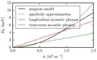
Figure 1: Dispersion relations of the acoustic phonons and magnons in YIG at zero magnetic field.

III Magnon-phonon interactions

We derive in this section the magnon-phonon interactions due to the anisotropy and exchange interactions for a cubic lattice ferromagnet.

III.1 Phenomenological magnon-phonon interaction

In the long-wavelength/continuum limit ($k\lesssim k_{0}$) the magnetoelastic energy to lowest order in the deviations of magnetization and lattice from equilibrium reads [28, 23, 24, 25, 26]

$$E_{me}= \frac{n}{M_{s}^{2}}\int d^{3}r\sum_{\alpha\beta}\left[B_{\alpha\beta}M_{\alpha}(\mathbf{r})M_{\beta}(\mathbf{r})\right.$$

$$\left.+B^{\prime}_{\alpha\beta}\frac{\partial\mathbf{M}(\mathbf{r})}{\partial r_{\alpha}}\cdot\frac{\partial\mathbf{M}(\mathbf{r})}{\partial r_{\beta}}\right]X_{\alpha\beta}(\mathbf{r}),$$ (19)

where $n=1/a^{3}$. The strain tensor $X_{\alpha\beta}$ is defined in terms of the lattice displacements $X_{\alpha}$,

$$X_{\alpha\beta}(\mathbf{r})=\frac{1}{2}\left[\frac{\partial X_{\alpha}(\mathbf{r})}{\partial r_{\beta}}+\frac{\partial X_{\beta}(\mathbf{r})}{\partial r_{\alpha}}\right],$$ (20)

with, for a cubic lattice [28],

$$B_{\alpha\beta} =\delta_{\alpha\beta}B_{\parallel}+(1-\delta_{\alpha\beta})B_{\perp},$$ (21)

$$B^{\prime}_{\alpha\beta} =\delta_{\alpha\beta}B^{\prime}_{\parallel}+(1-\delta_{\alpha\beta})B^{\prime}_{\perp}.$$ (22)

$B_{\alpha\beta}$ is caused by magnetic anisotropies and $B_{\alpha\beta}^{\prime}$ by the exchange interaction under lattice deformations. For YIG at room temperature [27, 33]

$$B_{\parallel} =k_{B}\times 47.8\;\mathrm{K}=4.12\;\mathrm{meV},$$ (23)

$$B_{\perp} =k_{B}\times 95.6\;\mathrm{K}=8.24\;\mathrm{meV},$$ (24)

$$B_{\parallel}^{\prime}/a^{2} =k_{B}\times 2727\;\mathrm{K}=235\;\mathrm{meV},$$ (25)

$$B_{\perp}^{\prime}/a^{2} \approx 0.$$ (26)

We discuss the values for $B_{\parallel}^{\prime}$ and $B^{\prime}_{\perp}$ in Sec. III.3.

III.2 Anisotropy-mediated magnon-phonon interaction

The magnetoelastic anisotropy (19) is described by the Hamiltonian [28],

$$\mathcal{H}_{mp}^{an} =\sum_{\mathbf{q}\lambda}\left[\Gamma_{\mathbf{q}\lambda}b_{-\mathbf{q}}X_{\mathbf{q}\lambda}+\Gamma_{-\mathbf{q}\lambda}^{*}b_{\mathbf{q}}^{\dagger}X_{\mathbf{q}\lambda}\right]$$

$$+\frac{1}{\sqrt{N}}\sum_{\mathbf{q},\mathbf{k},\mathbf{k}^{\prime}}\delta_{\mathbf{k}-\mathbf{k}^{\prime}-\mathbf{q},0}\sum_{\lambda}\Gamma_{\mathbf{kk}^{\prime},\lambda}^{an}b_{\mathbf{k}}^{\dagger}b_{\mathbf{k}^{\prime}}X_{\mathbf{q}\lambda}$$

$$+\frac{1}{\sqrt{N}}\sum_{\mathbf{q},\mathbf{k},\mathbf{k}^{\prime}}\delta_{\mathbf{k}+\mathbf{k}^{\prime}+\mathbf{q},0}\sum_{\lambda}\Gamma_{\mathbf{kk}^{\prime},\lambda}^{bb}b_{\mathbf{k}}b_{\mathbf{k}^{\prime}}X_{\mathbf{q}\lambda}$$

$$+\frac{1}{\sqrt{N}}\sum_{\mathbf{q},\mathbf{k},\mathbf{k}^{\prime}}\delta_{\mathbf{k}+\mathbf{k}^{\prime}-\mathbf{q},0}\sum_{\lambda}\Gamma_{\mathbf{kk}^{\prime},\lambda}^{\bar{b}\bar{b}}b_{\mathbf{k}}^{\dagger}b_{\mathbf{k}^{\prime}}^{\dagger}X_{\mathbf{q}\lambda},$$ (27)

with interaction vertices

$$\Gamma_{\mathbf{q}\lambda} =\frac{B_{\perp}}{\sqrt{2S}}\left[iq_{z}e_{\mathbf{q}\lambda}^{x}+q_{z}e_{\mathbf{q}\lambda}^{y}\right.$$

$$\left.+\left(iq_{x}+q_{y}\right)e_{\mathbf{q}\lambda}^{z}\right],$$ (28)

$$\Gamma_{\mathbf{kk}^{\prime},\lambda}^{an} =U_{\mathbf{k}-\mathbf{k}^{\prime},\lambda},$$ (29)

$$\Gamma_{\mathbf{kk}^{\prime},\lambda}^{bb} =V_{-\mathbf{k}-\mathbf{k}^{\prime},\lambda},$$ (30)

$$\Gamma_{\mathbf{kk}^{\prime},\lambda}^{\bar{b}\bar{b}} =V_{-\mathbf{k}-\mathbf{k}^{\prime},\lambda}^{*},$$ (31)

and

$$U_{\mathbf{q},\lambda} =\frac{iB_{\parallel}}{S}\left[q_{x}e_{\mathbf{q}\lambda}^{x}+q_{y}e_{\mathbf{q}\lambda}^{y}-2q_{z}e_{\mathbf{q}\lambda}^{z}\right],$$ (32)

$$V_{\mathbf{q},\lambda} =\frac{iB_{\parallel}}{S}\left[q_{x}e_{\mathbf{q}\lambda}^{x}-q_{y}e_{\mathbf{q}\lambda}^{y}\right]$$

$$+\frac{B_{\perp}}{S}\left[q_{y}e_{\mathbf{q}\lambda}^{x}+q_{x}e_{\mathbf{q}\lambda}^{y}\right].$$ (33)

The one magnon-two phonon process is of the same order in the total number of magnons and phonons as the two magnon-one phonon processes, but its effect on magnon transport is small, as shown in Appendix B.

III.3 Exchange-mediated magnon-phonon interaction

The exchange-mediated magnon-phonon interaction is obtained under the assumption that the exchange interaction $J_{ij}$ between two neighboring spins at lattice sites $\mathbf{r}_{i}$ and $\mathbf{r}_{j}$ depends only on their distance, which leads to the expansion to leading order in the small parameter $(|\mathbf{r}_{i}-\mathbf{r}_{j}|-a)$

$$J_{ij}=J(|\mathbf{r}_{i}-\mathbf{r}_{j}|)\approx J+J^{\prime}\cdot(|\mathbf{r}_{i}-\mathbf{r}_{j}|-a),$$ (34)

where $a$ is the equilibrium distance and $J^{\prime}=\partial J/\partial a$. With $\mathbf{r}_{i}=\mathbf{R}_{i}+\mathbf{X}_{\mathbf{R}_{i}},$ the Heisenberg Hamiltonian (1) is modulated by

$$\mathcal{H}_{mp}^{ex}=-J^{\prime}\sum_{i}\sum_{\alpha=x,y,z}\left(X_{\mathbf{R}_{i}+a\mathbf{e}_{\alpha}}^{\alpha}-X_{\mathbf{R}_{i}}^{\alpha}\right)\mathbf{S}_{\mathbf{R}_{i}}\cdot\mathbf{S}_{\mathbf{R}_{i}+a\mathbf{e}_{\alpha}},$$ (35)

where $\mathbf{e}_{\alpha}$ is a unit vectors in the $\alpha$ direction. Expanding the displacements in terms of the phonon and magnon modes

$$\mathcal{H}_{mp}^{ex}=\frac{1}{\sqrt{N}}\sum_{\mathbf{q},\mathbf{k},\mathbf{k}^{\prime}}\delta_{\mathbf{k}-\mathbf{k}^{\prime}-\mathbf{q},0}\sum_{\lambda}\Gamma_{\mathbf{kk}^{\prime},\lambda}^{ex}b_{\mathbf{k}}^{\dagger}b_{\mathbf{k}^{\prime}}X_{\mathbf{q}\lambda},$$ (36)

with interaction

$$\Gamma_{\mathbf{kk}^{\prime},\lambda}^{ex} =8iJ^{\prime}S\sum_{\alpha}e_{\mathbf{k}-\mathbf{k}^{\prime},\lambda}^{\alpha}\sin\left(\frac{k_{\alpha}a}{2}\right)\sin\left(\frac{k^{\prime}_{\alpha}a}{2}\right)$$

$$\times\sin\left(\frac{(k_{\alpha}-k^{\prime}_{\alpha})a}{2}\right)$$

$$\approx iJ^{\prime}a^{3}S\sum_{\alpha}e_{\mathbf{k}-\mathbf{k}^{\prime},\lambda}^{\alpha}k_{\alpha}k_{\alpha^{\prime}}\left(k_{\alpha}-k^{\prime}_{\alpha}\right),$$ (37)

where the last line is the long-wavelength expansion. The magnon-phonon interaction

$$\Gamma_{\mathbf{k},\mathbf{k}^{\prime},\lambda}^{\bar{b}b}=\Gamma_{\mathbf{k},\mathbf{k}^{\prime},\lambda}^{ex}+\Gamma_{\mathbf{k},\mathbf{k}^{\prime},\lambda}^{an}$$ (38)

conserves the magnon number, while (30) and (31) do not. Phonon numbers are not conserved in either case.

The value of $J^{\prime}$ for YIG is determined by the magnetic Grüneisen parameter [32, 33]

$$\Gamma_{m}=\frac{\partial\ln T_{C}}{\partial\ln V}=\frac{\partial\ln J}{\partial\ln V}=\frac{J^{\prime}a}{3J},$$ (39)

where $V=Na^{3}$ is the volume of the magnet. The only assumption here is that the Curie temperature $T_{C}$ scales linearly with the exchange constant $J$ [43]. $\Gamma_{m}$ has been measured for YIG via the compressibility to be $\Gamma_{m}=-3.26$ [32], and via thermal expansion, $\Gamma_{m}=-3.13$ [33], so we set $\Gamma_{m}=-3.2$. For other materials the magnetic Grüneisen parameter is also of the order of unity and in many cases $\Gamma_{m}\approx-10/3$ [32, 44, 33]. A recent ab initio study of YIG finds $\Gamma_{m}=-3.1$ [45].

Comparing the continuum limit of Eq. (35) with the classical magnetoelastic energy (19)

$$B_{\parallel}^{\prime}=3\Gamma_{m}JS^{2}a^{2}/2,$$ (40)

where for YIG $B_{\parallel}^{\prime}/a^{2}\approx 235\;\mathrm{meV}$. We disregard $B_{\perp}^{\prime}$ since it vanishes for nearest neighbor interactions by cubic lattice symmetry.

The coupling strength of the exchange-mediated magnon-phonon interaction can be estimated from the exchange energy $SJ^{\prime}a\approx E_{ex}=SJ$ [46, 31] following Akhiezer et al. [47, 48]. Our estimate of $SJ^{\prime}a=3\Gamma_{m}SJ$ is larger by $3\Gamma_{m}$, i.e. one order of magnitude. Since the scattering rate is proportional to the square of the interaction strength, our estimate of the scattering rate is a factor $100$ larger than previous ones. The assumption $J^{\prime}a\approx J$ is too small to be consistent with the experimental Grüneisen constant [32, 33]. Ref. [3] educatedly guessed $J^{\prime}a\approx 100J,$ which we now judge to be too large.

III.4 Interaction vertices

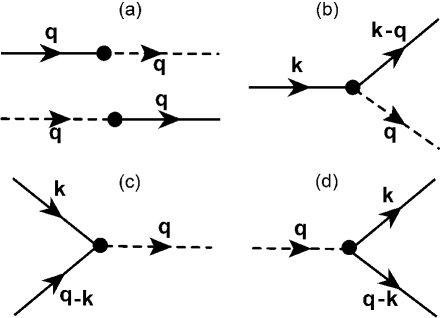
Figure 2: Feynman diagrams of interactions between magnons (solid lines) and phonons (dashed lines). The arrows indicate the energy-momentum flow. (a) magnon-phonon interconversion, (b) magnon number-conserving magnon-phonon interaction, (c) and (d) magnon number non-conserving magnon-phonon interactions.

The magnon-phonon interactions in the Hamiltonian (27) are shown in Fig. 2 as Feynman diagrams. Fig. 2(a) illustrates magnon and phonon interconversion, which is responsible for the magnon-phonon hybridization and level splitting at the crossing of magnon and phonon dispersions [27, 28]. The divergence of this diagram at the magnon-phonon crossing points is avoided by either direct diagonalization of the magnon-phonon Hamiltonian [42] or by cutting-off the divergence by a lifetime parameter [31]. This process still generates enhanced magnon transport that is observable as magnon polaron anomalies in the spin Seebeck effect [22] or spin-wave excitation thresholds [49, 50], but these are strongly localized in phase space and disregarded in the following, where we focus on the magnon scattering rates to leading order in $1/S$ of the scattering processes in Fig. 2(b)-(d).

IV Magnon scattering rate

Here we derive the magnon reciprocal quasi-particle lifetime $\tau_{qp}^{-1}=\gamma$ as the imaginary part of the wave vector dependent self-energy, caused by acoustic phonon scattering [28],

$$\gamma(\mathbf{k})=-\frac{2}{\hbar}\mathrm{Im}\Sigma(\mathbf{k},E_{\mathbf{k}}/\hbar+i0^{+}).$$ (41)

This quantity is in principle observable by inelastic neutron scattering. The total decay rate

$$\gamma=\gamma^{c}+\gamma^{nc}+\gamma^{\mathrm{other}}$$ (42)

is the sum of the magnon number conserving decay rate $\gamma^{c}$ and the magnon number non-conserving decay rate $\gamma^{nc}$, which are related to the magnon-phonon scattering time $\tau_{mp}$ and the magnon-phonon dissipation time $\tau_{mr}$ by

$$\tau_{mp}=\frac{1}{\gamma^{c}},\quad\tau_{mr}=\frac{1}{\gamma^{nc}}.$$ (43)

$\gamma^{\mathrm{other}}$ is caused by magnon-magnon and magnon disorder scattering, thereby beyond the scope of this work.

The self-energy to leading order in the $1/S$ expansion is of second order in the magnon-phonon interaction [28],

$$\Sigma_{2}(\mathbf{k},i\omega) =\frac{1}{N}\sum_{\mathbf{k^{\prime}}\lambda}\frac{\hbar^{2}\left|\Gamma_{\mathbf{k},\mathbf{k}^{\prime},\lambda}^{\bar{b}b}\right|^{2}}{2m\varepsilon_{\mathbf{k}-\mathbf{k}^{\prime},\lambda}}\left[\frac{n_{B}(\varepsilon_{\mathbf{k}-\mathbf{k}^{\prime},\lambda})-n_{B}(E_{\mathbf{k}^{\prime}})}{i\hbar\omega+\varepsilon_{\mathbf{k}-\mathbf{k}^{\prime},\lambda}-E_{\mathbf{k}^{\prime}}}+\frac{1+n_{B}(\varepsilon_{\mathbf{k}-\mathbf{k}^{\prime},\lambda})+n_{B}(E_{\mathbf{k}^{\prime}})}{i\hbar\omega-\varepsilon_{\mathbf{k}-\mathbf{k}^{\prime},\lambda}-E_{\mathbf{k}^{\prime}}}\right]$$

$$-\frac{1}{N}\sum_{\mathbf{k^{\prime}}\lambda}\frac{\hbar^{2}\left|\Gamma_{\mathbf{k},\mathbf{k}^{\prime},\lambda}^{bb}\right|^{2}}{2m\varepsilon_{\mathbf{k}-\mathbf{k}^{\prime},\lambda}}\left[\frac{1+n_{B}(\varepsilon_{\mathbf{k}+\mathbf{k}^{\prime},\lambda})+n_{B}(E_{\mathbf{k}^{\prime}})}{i\hbar\omega+\varepsilon_{\mathbf{k}+\mathbf{k}^{\prime},\lambda}+E_{\mathbf{k}^{\prime}}}+\frac{n_{B}(\varepsilon_{\mathbf{k}+\mathbf{k}^{\prime},\lambda})-n_{B}(E_{\mathbf{k}^{\prime}})}{i\hbar\omega-\varepsilon_{\mathbf{k}+\mathbf{k}^{\prime},\lambda}+E_{\mathbf{k}^{\prime}}}\right],$$ (44)

where the magnon number conserving magnon-phonon scattering vertex $\Gamma_{\mathbf{k},\mathbf{k}^{\prime},\lambda}^{\bar{b}b}=\Gamma_{\mathbf{k},\mathbf{k}^{\prime},\lambda}^{ex}+\Gamma_{\mathbf{k},\mathbf{k}^{\prime},\lambda}^{an}$ and the Planck (Bose) distribution function $n_{B}(\varepsilon)=(e^{\beta\varepsilon}-1)^{-1}$ with inverse temperature $\beta=1/(k_{B}T)$. The Feynman diagrams representing the magnon number conserving and non-conserving contributions to the self-energy are shown in Fig. 3.

Figure 3: Feynman diagrams representing the self-energy Eq. (44) due to (a) magnon number-conserving magnon-phonon interactions and (b) magnon number non-conserving magnon-phonon interactions.

We write the decay rate in terms of four contributions

$$\gamma(\mathbf{k})=\gamma_{out}^{c}(\mathbf{k})+\gamma_{out}^{nc}(\mathbf{k})-\gamma_{in}^{c}(\mathbf{k})-\gamma_{in}^{nc}(\mathbf{k}),$$ (45)

where $out$ and $in$ denote the out-scattering and in-scattering parts. The contributions to the decay rate read [28]

$$\gamma_{out}^{c}(\mathbf{k})= \frac{\pi\hbar}{mN}\sum_{\mathbf{q},\lambda}\frac{\left|\Gamma_{\mathbf{k},\mathbf{k}-\mathbf{q},\lambda}^{\bar{b}b}\right|^{2}}{\varepsilon_{\mathbf{q}\lambda}}\left[(1+n_{B}(E_{\mathbf{k}-\mathbf{q}}))n_{B}(\varepsilon_{\mathbf{q}\lambda})\delta(E_{\mathbf{k}}-E_{\mathbf{k}-\mathbf{q}}+\varepsilon_{\mathbf{q}\lambda})\right.$$

$$\phantom{{+\sum_{\mathbf{q},\lambda}\frac{\left|\Gamma_{\mathbf{k},\mathbf{k}-\mathbf{q},\lambda}^{\bar{b}b}\right|^{2}}{\varepsilon_{\mathbf{q}\lambda}}\}}}+\left.(1+n_{B}(E_{\mathbf{k}-\mathbf{q}}))(1+n_{B}(\varepsilon_{\mathbf{q}\lambda}))\delta(E_{\mathbf{k}}-E_{\mathbf{k}-\mathbf{q}}-\varepsilon_{\mathbf{q}\lambda})\right],$$ (46)

$$\gamma_{in}^{c}(\mathbf{k})= \frac{\pi\hbar}{mN}\sum_{\mathbf{q},\lambda}\frac{\left|\Gamma_{\mathbf{k},\mathbf{k}-\mathbf{q},\lambda}^{\bar{b}b}\right|^{2}}{\varepsilon_{\mathbf{q}\lambda}}\left[n_{B}(E_{\mathbf{k}-\mathbf{q}})(1+n_{B}(\varepsilon_{\mathbf{q}\lambda}))\delta(E_{\mathbf{k}}-E_{\mathbf{k}-\mathbf{q}}+\varepsilon_{\mathbf{q}\lambda})\right.$$

$$\phantom{{+\sum_{\mathbf{q},\lambda}\frac{\left|\Gamma_{\mathbf{k},\mathbf{k}-\mathbf{q},\lambda}^{\bar{b}b}\right|^{2}}{\varepsilon_{\mathbf{q}\lambda}}\}}}+\left.n_{B}(E_{\mathbf{k}-\mathbf{q}})n_{B}(\varepsilon_{\mathbf{q}\lambda})\delta(E_{\mathbf{k}}-E_{\mathbf{k}-\mathbf{q}}-\varepsilon_{\mathbf{q}\lambda})\right],$$ (47)

$$\gamma_{out}^{nc}(\mathbf{k})= \frac{\pi\hbar}{mN}\sum_{\mathbf{q},\lambda}\frac{\left|\Gamma_{\mathbf{k},\mathbf{q}-\mathbf{k},\lambda}^{bb}\right|^{2}}{\varepsilon_{\mathbf{q}\lambda}}\left[n_{B}(E_{\mathbf{q}-\mathbf{k}})(1+n_{B}(\varepsilon_{\mathbf{q}\lambda}))\delta(E_{\mathbf{k}}+E_{\mathbf{q}-\mathbf{k}}-\varepsilon_{\mathbf{q}\lambda})\right],$$ (48)

$$\gamma_{in}^{nc}(\mathbf{k})= \frac{\pi\hbar}{mN}\sum_{\mathbf{q},\lambda}\frac{\left|\Gamma_{\mathbf{k},\mathbf{q}-\mathbf{k},\lambda}^{bb}\right|^{2}}{\varepsilon_{\mathbf{q}\lambda}}\left[(1+n_{B}(E_{\mathbf{q}-\mathbf{k}}))n_{B}(\varepsilon_{\mathbf{q}\lambda})\delta(E_{\mathbf{k}}+E_{\mathbf{q}-\mathbf{k}}-\varepsilon_{\mathbf{q}\lambda})\right],$$ (49)

where the sum is over all momenta $\mathbf{q}$ in the Brillouin zone. Here the magnon/phonon annihilation rate is proportional to the Boson number $n_{B}$, while the creation rate scales with $1+n_{B}$. For example, in the out-scattering rate $\gamma_{out}^{c}(\mathbf{k})$ the incoming magnon with momentum $\mathbf{k}$ gets scattered into the state $\mathbf{k}-\mathbf{q}$ and a phonon is either absorbed with probability $\sim n_{B}$ or emitted with probability $\sim(1+n_{B})$. The out- and in-scattering rates are related by the detailed balance

$$\gamma_{in}^{c}(\mathbf{k})/\gamma_{out}^{c}(\mathbf{k})=\gamma_{in}^{nc}(\mathbf{k})/\gamma_{out}^{nc}(\mathbf{k})=e^{-\beta E_{\mathbf{k}}}.$$ (50)

For high temperatures $k_{B}T\gg E_{\mathbf{k}}$, we may expand the Bose functions $n_{B}(E_{\mathbf{k}})\sim k_{B}T/E_{\mathbf{k}}$ and we find $\gamma_{in}\sim\gamma_{out}\sim T^{2}$ and $\gamma=\gamma_{out}-\gamma_{in}\sim T$. For low temperatures $k_{B}T\ll E_{\mathbf{k}}$, the out-scattering rate $\gamma_{out}\to\mathrm{const}.$ and the in-scattering rate $\gamma_{in}\sim e^{-\beta E_{\mathbf{k}}}\to 0$. The scattering processes (c) and (d) in Fig. 2 conserve energy and linear momentum, but not angular momentum. A loss of angular momentum after integration over all wave vectors corresponds to a mechanical torque on the total lattice that contributes to the Einstein-de Haas effect [51].

V Magnon transport lifetime

In this section we compare the transport lifetime $\tau_{t}$ and the magnon quasi-particle lifetime $\tau_{qp}$ that can be very different [52, 53, 54], but, to the best of our knowledge, has not yet been addressed for magnons. The magnon decay rate is proportional to the imaginary part of self energy, as shown in Eq. (41). On the other hand, the transport is governed by transport lifetime $\tau_{t}$ in the Boltzmann equation that agrees with $\tau_{qp}$ only in the relaxation time approximation. The stationary Boltzmann equation for the magnon distribution can be written as [3, 42]

$$\frac{\partial f_{\mathbf{k}}(\mathbf{r})}{\partial\mathbf{r}}\cdot\frac{\partial E_{\mathbf{k}}}{\partial(\hbar\mathbf{k})}=\Gamma_{in}[f]-\Gamma_{out}[f],$$ (51)

where $f_{\mathbf{k}}(\mathbf{r})$ is the magnon distribution function. The $in$ and $out$ contributions to the collision integral are related to the previously defined in- and out-scattering rates by

$$\Gamma_{in}[f] =(1+f_{\mathbf{k}})\gamma_{in}[f],$$ (52)

$$\Gamma_{out}[f] =f_{\mathbf{k}}\gamma_{out}[f],$$ (53)

where the equilibrium magnon distribution $n_{B}(E_{\mathbf{k}})$ is replaced by the non-equilibrium distribution function $f_{\mathbf{k}}$. The factor $(1+f_{\mathbf{k}})$ corresponds to the creation of a magnon with momentum $\mathbf{k}$ in the in-scattering process and the factor $f_{\mathbf{k}}$ to the annihilation in the out-scattering process. The phonons are assumed to remain at thermal equilibrium, so we disregard the phonon drift contribution that is expected in the presence of a phononic heat current.

Magnon transport is governed by three linear response functions, i.e. spin and heat conductivity and spin Seebeck coefficient [42]. These can be obtained from the expansion of the distribution function in terms of temperature and chemical potential gradients and correspond to two-particle Green functions with vertex corrections, that reflect the non-equilibrium in-scattering processes, captured by a transport lifetime $\tau_{t}$ that can be different from the quasi-particle (dephasing) lifetime $\tau_{qp}$ defined by the self-energy. We define the transport life time of a magnon with momentum $\mathbf{k}$ in terms of the collision integral

$$\Gamma_{out}[f]-\Gamma_{in}[f]=\frac{1}{\tau_{\mathbf{k},t}[f]}\left(f_{\mathbf{k}}(\mathbf{r})-f_{0,\mathbf{k}}\right),$$ (54)

with $f_{0,\mathbf{k}}=n_{B}(E_{\mathbf{k}})$ and we assume a thermalized quasi-equilibrium distribution function

$$f_{\mathbf{k}}(\mathbf{r})=n_{B}\left(\frac{E_{\mathbf{k}}-\mu(\mathbf{r})}{k_{B}T(\mathbf{r})}\right),$$ (55)

where $\mu$ is the magnon chemical potential. We linearize the function $f_{\mathbf{k}}$ in terms of small deviations $\delta f_{\mathbf{k}}$ from equilibrium $f_{0,\mathbf{k}}$,

$$\delta f_{\mathbf{k}}=f_{\mathbf{k}}-f_{0,\mathbf{k}}.$$ (56)

leading to [3]

$$\delta f_{\mathbf{k}}=\tau_{\mathbf{k},t}\left[f\right]\frac{\partial f_{0,\mathbf{k}}}{\partial E_{\mathbf{k}}}\frac{\partial E_{\mathbf{k}}}{\partial(\hbar\mathbf{k})}\cdot\left(\boldsymbol{\nabla}\mu+\frac{E_{\mathbf{k}}-\mu}{T}\boldsymbol{\nabla}T\right),$$ (57)

where the gradients of chemical potential $\boldsymbol{\nabla}\mu$ and temperature $\boldsymbol{\nabla}T$ drive the magnon current. In the relaxation time approximation we disregard the dependence of $\tau_{\mathbf{k},t}[f]$ on $\delta f$ and recover the quasi-particle lifetime $\tau_{\mathbf{k},t}\rightarrow\tau_{\mathbf{k},qp}$.

To first order in the phonon operators and second order in the magnon operators the collision integral for magnon number non-conserving processes,

$$\Gamma_{out}^{nc}[f]-\Gamma_{in}^{nc}[f]$$

$$=\frac{\pi\hbar}{mN}\sum_{\mathbf{q}\lambda}\frac{|\Gamma_{\mathbf{k},\mathbf{\mathbf{q}-\mathbf{k}},\lambda}^{bb}|^{2}}{\varepsilon_{\mathbf{q}\lambda}}\delta(E_{\mathbf{k}}+E_{\mathbf{\mathbf{q}-\mathbf{k}}}-\varepsilon_{\mathbf{q}\lambda})$$

$$\times\left[(1+n_{\mathbf{q}\lambda})f_{\mathbf{k}}f_{\mathbf{q}-\mathbf{k}}-n_{\mathbf{\mathbf{q}\lambda}}(1+f_{\mathbf{q}-\mathbf{k}})(1+f_{\mathbf{k}})\right],$$ (58)

where the interaction vertex $\Gamma_{\mathbf{k},\mathbf{k^{\prime}},\lambda}^{bb}$ is given by Eq. (30) and $n_{\mathbf{\mathbf{q}\lambda}}=n_{B}(\varepsilon_{\mathbf{\mathbf{q}\lambda}})$. By using the expansion (56) in the collision integral that vanishes at equilibrium,

$$\Gamma_{out}[f_{0}]-\Gamma_{in}[f_{0}]=0,$$ (59)

we arrive at

$$\frac{1}{\tau_{\mathbf{k},t}^{nc}} =\frac{\pi\hbar}{mN}\sum_{\mathbf{q}\lambda}\frac{|\Gamma_{\mathbf{k},\mathbf{\mathbf{q}-\mathbf{k}},\lambda}^{bb}|^{2}}{\varepsilon_{\mathbf{q}\lambda}}\delta(E_{\mathbf{k}}+E_{\mathbf{\mathbf{q}-\mathbf{k}}}-\varepsilon_{\mathbf{q}\lambda})$$

$$\times\left[n_{B}(E_{\mathbf{k-q}})-n_{\mathbf{\mathbf{q}\lambda}}+\frac{\delta f_{\mathbf{\mathbf{q}-\mathbf{k}}}}{\delta f_{\mathbf{k}}}(n_{B}(E_{\mathbf{k}})-n_{\mathbf{q}\lambda})\right].$$ (60)

For the magnon number conserving process the derivation is similar and we find

$$\frac{1}{\tau_{\mathbf{k},t}^{c}} =\frac{\pi\hbar}{mN}\sum_{\mathbf{q}\lambda}\frac{|\Gamma_{\mathbf{k},\mathbf{\mathbf{k}-\mathbf{q}},\lambda}^{\bar{b}b}|^{2}}{\varepsilon_{\mathbf{q}\lambda}}\Bigg{[}\delta(E_{\mathbf{k}}-E_{\mathbf{\mathbf{k}-\mathbf{q}}}+\varepsilon_{\mathbf{q}\lambda})$$

$$\times \left(n_{\mathbf{q}\lambda}-n_{B}(E_{\mathbf{k-q}})-\frac{\delta f_{\mathbf{k}-\mathbf{q}}}{\delta f_{\mathbf{k}}}(n_{B}(E_{\mathbf{k}})+n_{\mathbf{\mathbf{q}\lambda}}+1)\right)$$

$$+ \delta(E_{\mathbf{k}}-E_{\mathbf{\mathbf{k}-\mathbf{q}}}-\varepsilon_{\mathbf{q}\lambda})$$

$$\times \left(1+n_{B}(E_{\mathbf{k-q}})+n_{\mathbf{\mathbf{q}\lambda}}+\frac{\delta f_{\mathbf{\mathbf{k}-\mathbf{q}}}}{\delta f_{\mathbf{k}}}(n_{B}(E_{\mathbf{k}})-n_{\mathbf{q}\lambda})\right)\Bigg{]},$$

with interaction vertex $\Gamma_{\mathbf{k},\mathbf{k^{\prime}},\lambda}^{\bar{b}b}$ given by Eq. (38). Due to the $\delta f_{\mathbf{\mathbf{k}-\mathbf{q}}}/\delta f_{\mathbf{k}}$ term this is an integral equation. It can be solved iteratively to generate a geometric series referred to as vertex correction in diagrammatic theories. By simply disregarding the in-scattering with terms $\delta f_{\mathbf{\mathbf{k}-\mathbf{q}}}/\delta f_{\mathbf{k}}$ the transport lifetime reduces to the the quasi-particle lifetime of the self-energy. We leave the general solution of this integral equation for future work, but argue in Sec. VI.4 that the vertex corrections are not important in our regime of interest.

VI Numerical results

VI.1 Magnon decay rate

In the following we present and analyze our results for the magnon decay rates in YIG. We first consider the case of vanishing effective magnetic field ($B=0$) and discuss the magnetic field dependence in Sec. VI.3. Since our model is only valid in the long-wavelength ($k<8\text{\texttimes}10^{8}\;\mathrm{m}^{-1}$) and low-temperature ($T\lesssim 100\;\mathrm{K}$) regime, we focus first on $T=50\;\mathrm{K}$ and discuss the temperature dependence in Sec. VI.2.

In Fig. 4 we show the magnon number conserving decay rate $\gamma^{c}(\mathbf{k})$, which is on the displayed scale dominated by the exchange-mediated magnon-phonon interaction and is isotropic for long-wavelength magnons.

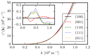
Figure 4: Magnon decay rate in YIG due to magnon-phonon interactions for magnons propagating along various directions at $T=50\;\mathrm{K}$ and $B=0$. We denote the propagation direction by $(lmn)$, i.e. $l\mathbf{e}_{x}+m\mathbf{e}_{y}+n\mathbf{e}_{z}$. The inset shows the relative deviation $\delta\gamma^{c}/\gamma^{c}$ from the (100) direction.

In Fig. 5 we compare the contribution from the exchange-mediated magnon-phonon interaction ($\gamma^{c}\sim k^{4}$) and from the anisotropy-mediated magnon-phonon interaction ($\gamma^{c}\sim k^{2}$). We observe a cross-over at $k\approx 4\times 10^{7}\;\mathrm{m}^{-1}$: for much smaller wave numbers, the exchange contribution can be disregarded and for larger wave numbers the exchange contribution becomes dominant.

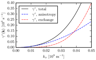
Figure 5: Comparison of the contributions from exchange-mediated and anisotropy-mediated magnon-phonon interactions to the magnon number conserving scattering rate $\gamma^{c}$ at $T=50\;\mathrm{K}$ and $B=0$.

The magnon number non-conserving decay rate $\gamma^{nc}$ in Fig. 6 is much smaller than the magnon-conserving one. This is consistent with the low magnetization damping of YIG, i.e. the magnetization is long-lived. We observe divergent peaks at the crossing points (shown in Fig. 1) with the exception of the (001) direction. These divergences occur when magnons and phonons are degenerate at $k=0.48\times 10^{9}\;\mathrm{m}^{-1}$ ($1.2\;\mathrm{meV}$) and $k=0.9\times 10^{9}\;\mathrm{m}^{-1}$ ($4.3\;\mathrm{meV}$), respectively, at which the Boltzmann formalism does not hold; a treatment in the magnon-polaron basis [42] or a broadening parameter [31] would get rid of the singular behavior. The divergences are also suppressed by arbitrarily small effective magnetic fields (see Sec. VI.3). There are no peaks along the (001) direction because in the (001) direction the vertex function $V_{\mathbf{q},\lambda}$ (see Eq. (33)) vanishes for $\mathbf{q}=(0,0,k_{z})$. For $k>\hbar c_{l}/(D(\sqrt{8}-2))=1.085\times 10^{9}\;\mathrm{m}^{-1}$ the decay rate $\gamma^{nc}$ vanishes because the decay process does not conserve energy ($\delta(E_{\mathbf{k}}+E_{\mathbf{q}-\mathbf{k}}-\varepsilon_{\mathbf{q}\lambda})=0$).

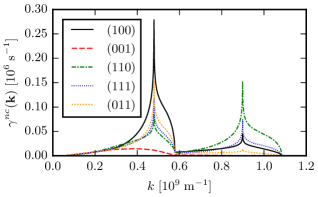
Figure 6: Magnon decay rate in YIG due to magnon number non-conserving magnon-phonon interactions for magnons propagating along various directions at $T=50\;\mathrm{K}$ and $B=0$.

VI.2 Temperature dependence

Above we focused on $T=50\;\mathrm{K}$ and explained that we expect a linear temperature dependence of the magnon decay rates at high, but not low temperatures. Fig. 7 shows our results for the temperature dependence at $k_{x}=10^{8}\;\mathrm{m}^{-1}$. Deviations from the linear dependence at low temperatures occurs when quantum effects set in, i.e. the Rayleigh-Jeans distribution does not hold anymore,

$$\frac{1}{e^{\varepsilon/(k_{B}T)}-1}\not\approx\frac{k_{B}T}{\varepsilon}.$$ (62)

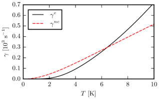
Figure 7: Temperature dependence of the magnon decay rates $\gamma^{nc}$ and $\gamma^{c}$ at $B=0$, $k_{x}=10^{8}\;\mathrm{m}^{-1}$ and $k_{y}=k_{z}=0$, i.e. along (100).

VI.3 Magnetic field dependence

The numerical results presented above are for a mono-domain magnet in the limit of small applied magnetic fields. A finite magnetic field $B$ along the magnetization direction induces an energy gap $g\mu_{B}B$ in the magnon dispersion, which shifts the positions of the magnon-phonon crossing points to longer wavelengths. The magnetic field suppresses the (unphysical) sharp peaks at the crossing points (see Fig. 8) that are caused by the divergence of the Planck distribution function for a vanishing spin wave gap.

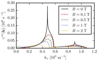
Figure 8: Magnetic field dependence of the magnon number non-conserving magnon decay rate in YIG at $T=50\;\mathrm{K}$ with magnon momentum along (100).

In the magnon number conserving magnon-phonon interactions, the magnetic field dependence cancels in the delta function and enters only in the Bose function via $n_{B}$ (magnetic freeze-out). Fig. 9 shows that the magnetic field mainly affects magnons with energies $\lesssim 2g\mu_{B}B=0.23(B/\mathrm{T})\;\mathrm{meV}$.

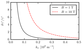
Figure 9: Relative deviation $\delta\gamma^{c}/\gamma^{c}$ from the $B=0$ result of the magnon number conserving magnon decay rate in YIG at $T=50\;\mathrm{K}$ with magnon momentum along (100).

As shown in Fig. 10 the magnon decay by phonons does not vanish for the $\mathbf{k}=0$ Kittel mode, but only in the presence of a spin wave gap $E_{0}=g\mu_{B}B$. Both magnon conserving and non-conserving scattering processes contribute. The divergent peaks at $B\approx 1.3\;\mathrm{T}$ and $B\approx 4.6\;\mathrm{T}$ in $\gamma^{nc}$ are caused by energy and momentum conservation in the two-magnon-one-phonon scattering process,

$$\delta(E_{\mathbf{k}=0}+E_{\mathbf{q}}-\varepsilon_{\mathbf{q}\lambda})=\delta(2g\mu_{B}B+E_{ex}q^{2}a^{2}-\hbar c_{\lambda}q),$$ (63)

when the gradient of the argument of the delta function vanishes,

$$\boldsymbol{\nabla}_{\mathbf{q}}(E_{\mathbf{k}=0}+E_{\mathbf{q}}-\varepsilon_{\mathbf{q}\lambda})=0,$$ (64)

i.e., the two-magnon energy $E_{\mathbf{k}=0}+E_{\mathbf{q}}$ touches either the transverse or longitudinal phonon dispersion $\varepsilon_{\mathbf{q}\lambda}$. The total energy of the two magnons is equivalent to the energy of a single magnon with momentum $q$ but in a field $2B$, resulting in the divergence at fields that are half of those for the magnon-polaron observed in the spin Seebeck effect [42, 31]. The two-magnon touching condition can be satisfied in all directions of the phonon momentum $\mathbf{q}$, which therefore contributes to the magnon decay rate when integrating over the phonon momentum $\mathbf{q}$. For $\mathbf{k}\neq 0$ this two-magnon touching condition can only be fulfilled for phonons along a particular direction and the divergence is suppressed.

The magnon decay rate is related to the Gilbert damping $\alpha_{\mathbf{k}}$ as $\hbar\gamma_{\mathbf{k}}=2\alpha_{\mathbf{k}}E_{\mathbf{k}}$ [55]. We find that phonons contribute only weakly to the Gilbert damping, $\alpha_{0}^{nc}=\hbar\gamma_{0}^{nc}/(2E_{0})\sim 10^{-8}$ at $T=50\;\mathrm{K}$, which is much smaller than the total Gilbert damping $\alpha\sim 10^{-5}$ in YIG, but the peaks at $1.3\;\mathrm{T}$ and $4.6\;\mathrm{T}$ might be observable. The phonon contribution to the Gilbert damping scales linearly with temperature, so is twice as large at 100 K. At low temperatures ($T\lesssim 100\;\mathrm{K}$) Gilbert damping in YIG has been found to be caused by two-level systems [56] and impurity scattering [40], while for higher temperatures magnon-phonon [57] and magnon-magnon scattering involving optical magnons [34] have been proposed to explain the observed damping. Enhanced damping as a function of magnetic field at higher temperatures might reveal other van Hove singularities in the joint magnon-phonon density of states.

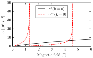
Figure 10: Magnetic field dependence of the magnon decay rates in YIG at $\mathbf{k}=0$ and $T=50\;\mathrm{K}$.

VI.4 Magnon transport lifetime

We do not attempt a full solution of the integral equations (60) and (LABEL:eq:tau_t^c) for the transport lifetime. However, we can still estimate its effect by the observation that the ansatz $\tau_{\mathbf{k},t}^{-1}\sim k^{n}$ can be an approximate solution of the Boltzmann equation with in-scattering.

Our results for the magnon number conserving interaction are shown in Fig. 11 (for $\boldsymbol{\nabla}T=0$ and finite $\boldsymbol{\nabla}\mu||\mathbf{e}_{x}$), where $\gamma_{t}=\tau_{t}^{-1}$. We consider the cases $n=0,2,4$, where $n=0$ or $\tau_{\mathbf{k},t}=\mathrm{const}.$ would be the solution for a short-range scattering potential. For very long wavelengths ($k\lesssim 4\times 10^{7}\;\mathrm{m}^{-1}$) the inverse quasi-particle lifetime $\tau_{\mathbf{k},qp}^{-1}\sim k^{2}$ and for shorter wavelengths $\tau_{\mathbf{k},qp}^{-1}\sim k^{4}$. $n=2$ is a self-consistent solution only for very small $k\lesssim 4\times 10^{7}\;\mathrm{m}^{-1}$, while $\tau_{\mathbf{k},qp}^{-1}\sim k^{4}$ is a good ansatz up to $k\lesssim 0.3\times 10^{9}\;\mathrm{m}^{-1}$. We see that the transport lifetime approximately equals the quasi-particle lifetime in the regime of the validity of the $n=4$ power law.

For the magnon number non-conserving processes in Fig. 12 the quasi-particle lifetime behaves as $\tau_{\mathbf{k},qp}^{-1}\sim k^{2}$. The ansatz $n=2$ turns out to be self-consistent and we see deviations of the transport lifetime from the quasi-particle lifetime for $k\gtrsim 5\times 10^{7}\;\mathrm{m}^{-1}$. The plot only shows our results for $k<1\times 10^{8}\;\mathrm{m}^{-1}$ because our assumption of an isotropic lifetime is not valid for higher momenta in this case.

We conclude that for YIG in the long-wavelength regime the magnon transport lifetime (due to magnon-phonon interactions) should be approximately the same as the quasi-particle lifetime, but deviations at shorter wavelengths require more attention.

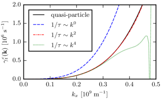
Figure 11: Inverse of the magnon transport lifetime in YIG (with magnon momentum along (100)) due to magnon number conserving magnon-phonon interactions at $T=50\;\mathrm{K}$ and $B=0$ for magnons along the (100) direction.

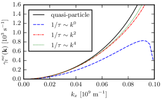
Figure 12: Inverse of the magnon transport lifetime in YIG (with magnon momentum along (100)) due to magnon number non-conserving interactions at $T=50\;\mathrm{K}$ and $B=0$.

VII Summary and conclusion

We calculated the decay rate of magnons in YIG induced by magnon-phonon interactions in the long-wavelength regime ($k\lesssim 1\times 10^{9}\;\mathrm{m}^{-1}$). Our model takes only the acoustic magnon and phonon branches into account and is therefore valid at low to intermediate temperatures ($T\lesssim 100\;\mathrm{K}$). The exchange-mediated magnon-phonon interaction has been recently identified as a crucial contribution to the overall magnon-phonon interaction in YIG at high temperatures [3, 29, 45]. We emphasize that its coupling strength can be derived from experimental values of the magnetic Grüneisen parameter $\Gamma_{m}=\partial\ln T_{C}/\partial\ln V$ [32, 33]. In previous works this interaction has been either disregarded [28], underestimated [29, 46], or overestimated [3].

In the ultra-long-wavelength regime the wave vector dependent magnon decay rate $\gamma(\mathbf{k})$ is determined by the anisotropy-mediated magnon-phonon interaction with $\gamma(\mathbf{k})\sim k^{2}$, while for shorter wavelengths $k\gtrsim 4\times 10^{7}\;\mathrm{m}^{-1}$ the exchange-mediated magnon-phonon interaction becomes dominant, which scales as $\gamma(\mathbf{k})\sim k^{4}$. The magnon number non-conserving processes are caused by spin-orbit interaction, i.e., the anisotropy-mediated magnon-phonon interaction, and are correspondingly weak.

In a finite magnetic field the average phonon scattering contribution, from the mechanism under study, to the Gilbert damping of the $k=0$ macrospin Kittel mode is about three orders of magnitude smaller than the best values for the Gilbert damping $\alpha\sim 10^{-5}$. However, we predict peaks at $1.3\;\mathrm{T}$ and $4.6\;\mathrm{T}$, that may be experimentally observable in high-quality samples.

The magnon transport lifetime, which is given by the balance between in- and out-scattering in the Boltzmann equation, is in the long-wavelength regime approximately the same as the quasi-particle lifetime. However, the magnon quasi-particle and transport lifetime differ more significantly at shorter wavelengths. A theory for magnon transport at room temperature should therefore include the “vertex corrections”.

A full theory of magnon transport at high temperature requires a method that takes the full dispersion relations of acoustic and optical phonons and magnons into account. This would also require a full microscopic description of the magnon-phonon interaction, since the magnetoelastic energy used here only holds in the continuum limit.

Appendix A Long-wavelength approximation

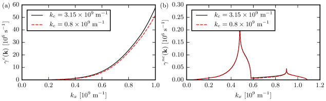
Figure 13: Dependence the magnon decay rate along (100) on the high magnon momentum cut-off $k_{c}$ for the (a) magnon number conserving ($\gamma^{c}$) and (b) non-conserving ($\gamma^{nc}$) contributions at $T=50\;\mathrm{K}$ and $B=0$.

The theory is designed for magnons with momentum $k<0.8\times 10^{9}\;\mathrm{m}^{-1}$ and phonons with momentum $q<2.5\times 10^{9}\;\mathrm{m}^{-1}$ (corresponding to phonon energies/frequencies $\leq$$12\;\mathrm{meV}$/$3\;\mathrm{THz}$), but relies on high-momentum cut-off parameters $k_{c}$ because of the assumption of quadratic/linear dispersion of magnon/phonons. We see in Fig. 13 that the scattering rates only weakly depend on $k_{c}$.

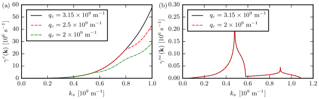
Figure 14: Dependence the magnon decay rate along (100) on the high phonon momentum cut-off $q_{c}$ for the (a) magnon number conserving ($\gamma^{c}$) and (b) non-conserving ($\gamma^{nc}$) contributions at $T=50\;\mathrm{K}$ and $B=0$.

The dependence of the scattering rate on the phonon momentum cut-off $q_{c}$ is shown in Fig. 14. $q_{c}=3.15\times 10^{9}\;\mathrm{m}^{-1}$ corresponds to an integration over the whole Brillouin zone, approximated by a sphere. From these considerations we estimate that the long-wavelength approximation is reliable for $k\lesssim 8\times 10^{8}\;\mathrm{m}^{-1}$. Optical phonons (magnons) that are thermally excited for $T\apprge 100\;\mathrm{K}\,(300\;\mathrm{K})$ are not considered here.

Appendix B Second order magnetoelastic coupling

The magnetoelastic energy is usually expanded only to first order in the displacement fields. Second order terms can become important e.g. when the first order terms vanish. This is the case for one-magnon two-phonon scattering processes. The first order term

$$\sum_{\mathbf{q}\lambda}\left[\Gamma_{\mathbf{q}\lambda}b_{-\mathbf{q}}X_{\mathbf{q}\lambda}+\Gamma_{-\mathbf{q}\lambda}^{*}b_{\mathbf{q}}^{\dagger}X_{\mathbf{q}\lambda}\right]$$ (65)

only contributes when phonon and magnon momenta and energies cross, giving rise to magnon polaron modes [42]. In other areas of reciprocal space the second order term should therefore be considered. Eastman [58, 59] derived the second-order magnetoelastic energy and determined the corresponding coupling constants for YIG. In momentum space, the relevant contribution to the Hamiltonian is of the form

$$\mathcal{H}_{2p1m} =\frac{1}{\sqrt{N}}\sum_{\mathbf{k},\mathbf{q}_{1},\lambda_{1},\mathbf{q}_{2},\lambda_{2}}$$

$$\left(\delta_{\mathbf{q}_{1}+\mathbf{q}_{2}+\mathbf{k},0}\Gamma_{\mathbf{q}_{1}\lambda_{1},\mathbf{q}_{2}\lambda_{2}}^{b}X_{\mathbf{q}_{1}\lambda_{1}}X_{\mathbf{q}_{2}\lambda_{2}}b_{\mathbf{k}}\right.$$

$$\left.+\delta_{\mathbf{q}_{1}+\mathbf{q}_{2}-\mathbf{k},0}\Gamma_{\mathbf{q}_{1}\lambda_{1},\mathbf{q}_{2}\lambda_{2}}^{\bar{b}}X_{\mathbf{q}_{1}\lambda_{1}}X_{\mathbf{q}_{2}\lambda_{2}}b_{\mathbf{k}}^{\dagger}\right),$$ (66)

where the interaction vertices are symmetrized,

$$\Gamma_{\mathbf{q}_{1}\lambda_{1},\mathbf{q}_{2}\lambda_{2}}^{b}=\frac{1}{2}\left(\tilde{\Gamma}_{\mathbf{q}_{1}\lambda_{1},\mathbf{q}_{2}\lambda_{2}}^{b}+\tilde{\Gamma}_{\mathbf{q}_{2}\lambda_{2},\mathbf{q}_{1}\lambda_{1}}^{b}\right),$$ (67)

and obey

$$\Gamma_{\mathbf{q}_{1}\lambda_{1},\mathbf{q}_{2}\lambda_{2}}^{b}=\left(\Gamma_{-\mathbf{q}_{1}\lambda_{1},-\mathbf{q}_{2}\lambda_{2}}^{\bar{b}}\right)^{*}.$$ (68)

The non-symmetrized vertex function is

$$\tilde{\Gamma}_{\mathbf{q}_{1}\lambda_{1},\mathbf{q}_{2}\lambda_{2}}^{b} =\frac{1}{a^{2}\sqrt{2S}}\left[B_{144}\left(iI_{1}-I_{1,x\leftrightarrow y}\right)\right.$$

$$+B_{155}\left(iI_{2}-I_{2,x\leftrightarrow y}\right)$$

$$+\left.B_{456}\left(iI_{3}-I_{3,x\leftrightarrow y}\right)\right],$$ (69)

with

$$I_{1} =a^{2}e_{\mathbf{q}_{1}\lambda_{1}}^{x}q_{1}^{x}\left[e_{\mathbf{q}_{2}\lambda_{2}}^{y}q_{2}^{z}+e_{\mathbf{q}_{2}\lambda_{2}}^{z}q_{2}^{y}\right],$$ (70)

$$I_{2} =a^{2}\left[e_{\mathbf{q}_{1}\lambda_{1}}^{y}q_{1}^{y}+e_{\mathbf{q}_{1}\lambda_{1}}^{z}q_{1}^{z}\right]$$

$$\times\left[e_{\mathbf{q}_{2}\lambda_{2}}^{y}q_{2}^{z}+e_{\mathbf{q}_{2}\lambda_{2}}^{z}q_{2}^{y}\right],$$ (71)

$$I_{3} =a^{2}\left[e_{\mathbf{q}_{1}\lambda_{1}}^{x}q_{1}^{z}+e_{\mathbf{q}_{1}\lambda_{1}}^{z}q_{1}^{x}\right]$$

$$\times\left[e_{\mathbf{q}_{2}\lambda_{2}}^{x}q_{2}^{y}+e_{\mathbf{q}_{2}\lambda_{2}}^{y}q_{2}^{x}\right],$$ (72)

and $x\leftrightarrow y$ denotes an exchange of $x$ and $y$. The relevant coupling constants in YIG are [59, 58]

$$B_{144} =-6\pm 48\;\mathrm{meV},$$ (73)

$$B_{155} =-44\pm 6\;\mathrm{meV},$$ (74)

$$B_{456} =-32\pm 8\;\mathrm{meV}.$$ (75)

The magnon self-energy (see Fig. 15) reads

$$\Sigma_{2p1m}(\mathbf{k},i\omega) =-\frac{2}{N}\sum_{\mathbf{q}_{1},\lambda_{1},\mathbf{q}_{2},\lambda_{2}}\frac{1}{\beta}\sum_{\Omega}\delta_{\mathbf{q}_{1}+\mathbf{q}_{2}+\mathbf{k},0}$$

$$\times\left|\Gamma_{\mathbf{q}_{1}\lambda_{1},\mathbf{q}_{2}\lambda_{2}}^{b}\right|^{2}F_{\lambda_{1}}(\mathbf{q}_{1},\Omega)F_{\lambda_{2}}(\mathbf{q}_{2},-\Omega-\omega).$$ (76)

with phonon propagator

$$F_{\lambda}(\mathbf{q},\Omega)=\frac{\hbar^{2}}{m}\frac{1}{\hbar^{2}\Omega^{2}+\varepsilon_{\mathbf{q}\lambda}^{2}}.$$ (77)

and leads to a magnon decay rate

$$\gamma_{2p}^{nc}(\mathbf{k}) =-\frac{2}{\hbar}\mathrm{Im}\Sigma_{2p1m}(\mathbf{k},i\omega\to E_{\mathbf{k}}/\hbar+i0^{+})$$

$$=\frac{\pi\hbar^{3}}{m^{2}N}\sum_{\mathbf{q}_{1},\lambda_{1},\mathbf{q}_{2},\lambda_{2}}\delta_{\mathbf{q}_{1}+\mathbf{q}_{2}+\mathbf{k},0}\frac{1}{\varepsilon_{1}\varepsilon_{2}}\left|\Gamma_{\mathbf{q}_{1}\lambda_{1},\mathbf{q}_{2}\lambda_{2}}^{b}\right|^{2}$$

$$\times\left\{2\delta\left(E_{\mathbf{k}}+\varepsilon_{1}-\varepsilon_{2}\right)\left[n_{1}-n_{2}\right]\right.$$

$$\left.+\delta\left(E_{\mathbf{k}}-\varepsilon_{1}-\varepsilon_{2}\right)\left[1+n_{1}+n_{2}\right]\right\},$$ (78)

where

$$n_{1} =n_{B}\left(\varepsilon_{\mathbf{q}_{1}\lambda_{1}}\right),\;n_{2}=n_{B}\left(\varepsilon_{\mathbf{q}_{2}\lambda_{2}}\right),$$ (79)

$$\varepsilon_{1} =\varepsilon_{\mathbf{q}_{1}\lambda_{1}},\;\varepsilon_{2}=\varepsilon_{\mathbf{q}_{2}\lambda_{2}}.$$ (80)

The first term in curly brackets on the right-hand-side of Eq. (78) describes annihilation and creation of a phonon as a sum of out-scattering minus in-scattering contributions,

$$n_{1}(1+n_{2})-(1+n_{1})n_{2}=n_{1}-n_{2},$$ (81)

while the second term can be understood in terms of out-scattering by the creation of two phonons and the in-scattering by annihilation of two phonons,

$$(1+n_{1})(1+n_{2})-n_{1}n_{2}=1+n_{1}+n_{2}.$$ (82)

For this one-magnon-two-phonon process the quasi-particle and the transport lifetimes are the same,

$$\tau_{t}=\tau_{qp},$$ (83)

since this process involves only a single magnon that is either annihilated or created. The collision integral is then independent of the magnon distribution of other magnons and the transport lifetime reduces to the quasi-particle lifetime.

The two-phonon contribution to the magnon scattering rate in YIG at $T=50\;\mathrm{K}$ and along (100) direction as shown in Fig. 16 is more than two orders of magnitude smaller than that from one-phonon processes and therefore disregarded in the main text. The numerical results depend strongly on the phonon momentum cutoff $q_{c}$, even in the long-wavelength regime, which implies that the magnons in this process dominantly interact with short-wavelength, thermally excited phonons. Indeed, the second order magnetoelastic interaction (69) is quadratic in the phonon momenta, which favors scattering with short-wavelength phonons. Our long-wavelength approximation therefore becomes questionable and the results may be not accurate at $T=50\;\mathrm{K}$, but this should not change the main conclusion that we can disregard these diagrams.

Our finding that the two-phonon contributions are so small can be understood in terms of the dimensionful prefactors of the decay rates (Eqs. (48-49) and (78)): The one-phonon decay rate is proportional to $\hbar/(ma^{2})\approx 7\times 10^{6}\;\mathrm{s^{-1}}$, while the two-phonon decay rate is proportional to $\hbar^{3}/(m^{2}a^{4}\varepsilon)\approx 33\;\mathrm{s}^{-1}$, where $\varepsilon\approx 1\;\mathrm{meV}$ is a typical phonon energy. The coupling constants for the magnon number non-conserving processes are $B_{\parallel,\perp}\sim 5\;\mathrm{meV}$ while the strongest two phonon coupling which enhances the two-phonon process by about a factor 100, but does not nearly compensate the prefactor. The two phonon process is therefore three orders of magnitudes smaller than the contribution of the one phonon process. The physical reason appears to be the large mass density of YIG, i.e. the heavy yttrium atoms.

Figure 15: Feynman diagram representing the self-energy Eq. (76) due to one-magnon-two-phonon processes.

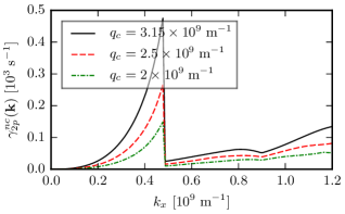
Figure 16: Two-phonon contribution to the magnon number non-conserving magnon scattering rate with magnon momentum along (100) for different values of the phonon momentum cutoff $q_{c}$ at $T=50\;\mathrm{K}$ and $B=0$.

Appendix C Numerical integration

The magnon decay rate is given be the weighted density of states

$$I=\int_{BZ}d^{3}q\,f(\mathbf{q})\delta\left(\varepsilon(\mathbf{q})\right),$$ (84)

that contain the Dirac delta function $\delta(\varepsilon)$ that can be eliminated to yield

$$I=\sum_{\mathbf{q}_{i}}\int_{A_{i}}d^{2}q\,\frac{f(\mathbf{q})}{\left|\mathbf{\nabla}\varepsilon(\mathbf{q})\right|},$$ (85)

where the $\mathbf{q}_{i}$ are the zeros of $\varepsilon(\mathbf{q})$ and $A_{i}$ the surfaces inside the Brillouin zone with $\varepsilon(\mathbf{q})=\varepsilon(\mathbf{q}_{i})$. The calculation these integrals is a standard numerical problem in condensed matter physics.

For a spherical Brillouin zone of radius $q_{c}$ and spherical coordinates $(q,\theta,\phi)$,

$$I=\int_{0}^{\pi}d\theta\int_{0}^{2\pi}d\phi\int_{0}^{q_{c}}dq\,q^{2}\sin(\theta)f(q,\theta,\phi)\delta\left(\varepsilon(q,\theta,\phi)\right).$$ (86)

When $\varepsilon(q_{i},\theta,\phi)=0$

$$\delta\left(\varepsilon(q,\theta,\phi)\right)=\sum_{q_{i}\left(\theta,\phi\right)}\frac{\delta\left(q-q_{i}\left(\theta,\phi\right)\right)}{\left|\varepsilon^{\prime}(q_{i}\left(\theta,\phi\right),\theta,\phi)\right|},$$ (87)

where $\varepsilon^{\prime}=\partial\varepsilon/\partial q$ and

$$I =\int_{0}^{\pi}d\theta\int_{0}^{2\pi}d\phi\,\sum_{q_{i}(\theta,\phi)<q_{c}}q_{i}^{2}(\theta,\phi)\sin(\theta)$$

$$\phantom{\int_{0}^{\pi}d\theta\int_{0}^{2\pi}d\phi\,\sum_{q_{i}(\theta,\phi)<q_{c}}}\times\frac{f(q_{i}\left(\theta,\phi\right),\theta,\phi)}{\left|\varepsilon^{\prime}(q_{i}\left(\theta,\phi\right),\theta,\phi)\right|},$$ (88)

which is particularly useful when the zeros of $\varepsilon(q,\theta,\phi)$ can be calculated analytically for linear and quadratic dispersion relations.

We can also evaluate the integral $I$ fully numerically by broadening the delta function [60] e.g. replacing it by a Gaussian [60],

$$\delta(\varepsilon)\to\frac{1}{\sqrt{\pi}\sigma}\exp\left(-\frac{\varepsilon^{2}}{\sigma^{2}}\right),$$ (89)

where $\sigma$ is the broadening parameter. An alternative is the Lorentzian (Cauchy-Lorentz distribution),

$$\delta(\varepsilon)\to\frac{1}{\pi\sigma}\frac{\sigma^{2}}{\varepsilon^{2}+\sigma^{2}},$$ (90)

which has fat tails that are helpful in finding the zeros of the delta function for an adaptive integration grid. Here we use the cubature package by Steven G. Johnson [61], which implements an adaptive multidimensional integration algorithm over hyperrectangular regions [62, 63].

References

- Serga et al. [2010] A. A. Serga, A. V. Chumak, and B. Hillebrands, J. Phys. D: Appl. Phys. 43, 264002 (2010).
- Kajiwara et al. [2010] Y. Kajiwara, K. Harii, S. Takahashi, J. Ohe, K. Uchida, M. Mizuguchi, H. Umezawa, H. Kawai, K. Ando, K. Takanashi, S. Maekawa, and E. Saitoh, Nature 464, 262 (2010).
- Cornelissen et al. [2016] L. J. Cornelissen, K. J. H. Peters, G. E. W. Bauer, R. A. Duine, and B. J. van Wees, Phys. Rev. B 94, 014412 (2016).
- Bauer et al. [2012] G. E. W. Bauer, E. Saitoh, and B. J. van Wees, Nat. Mater. 11, 391 (2012).
- Li et al. [2016] J. Li, Y. Xu, M. Aldosary, C. Tang, Z. Lin, S. Zhang, R. Lake, and J. Shi, Nat. Commun. 7, 10858 EP (2016).
- Cornelissen et al. [2015] L. J. Cornelissen, J. Liu, R. A. Duine, J. B. Youssef, and B. J. van Wees, Nat. Phys. 11, 1022 (2015), letter.
- Uchida et al. [2010a] K. Uchida, J. Xiao, H. Adachi, J. Ohe, S. Takahashi, J. Ieda, T. Ota, Y. Kajiwara, H. Umezawa, H. Kawai, G. E. W. Bauer, S. Maekawa, and E. Saitoh, Nat. Mater. 9, 894 (2010a).
- Uchida et al. [2010b] K. Uchida, H. Adachi, T. Ota, H. Nakayama, S. Maekawa, and E. Saitoh, Appl. Phys. Lett. 97, 172505 (2010b).
- Kikkawa et al. [2013] T. Kikkawa, K. Uchida, Y. Shiomi, Z. Qiu, D. Hou, D. Tian, H. Nakayama, X.-F. Jin, and E. Saitoh, Phys. Rev. Lett. 110, 067207 (2013).
- Siegel et al. [2014] G. Siegel, M. C. Prestgard, S. Teng, and A. Tiwari, Sci. Rep. 4, 4429 EP (2014).
- Jin et al. [2015] H. Jin, S. R. Boona, Z. Yang, R. C. Myers, and J. P. Heremans, Phys. Rev. B 92, 054436 (2015).
- Kehlberger et al. [2015] A. Kehlberger, U. Ritzmann, D. Hinzke, E.-J. Guo, J. Cramer, G. Jakob, M. C. Onbasli, D. H. Kim, C. A. Ross, M. B. Jungfleisch, B. Hillebrands, U. Nowak, and M. Kläui, Phys. Rev. Lett. 115, 096602 (2015).
- Iguchi et al. [2017] R. Iguchi, K. Uchida, S. Daimon, and E. Saitoh, Phys. Rev. B 95, 174401 (2017).
- Xiao et al. [2010] J. Xiao, G. E. W. Bauer, K. Uchida, E. Saitoh, and S. Maekawa, Phys. Rev. B 81, 214418 (2010).
- Adachi et al. [2011] H. Adachi, J.-i. Ohe, S. Takahashi, and S. Maekawa, Phys. Rev. B 83, 094410 (2011).
- Jaworski et al. [2011] C. M. Jaworski, J. Yang, S. Mack, D. D. Awschalom, R. C. Myers, and J. P. Heremans, Phys. Rev. Lett. 106, 186601 (2011).
- Adachi et al. [2013] H. Adachi, K. Uchida, E. Saitoh, and S. Maekawa, Rep. Prog. Phys. 76, 036501 (2013).
- Schreier et al. [2013] M. Schreier, A. Kamra, M. Weiler, J. Xiao, G. E. W. Bauer, R. Gross, and S. T. B. Goennenwein, Phys. Rev. B 88, 094410 (2013).
- Rezende et al. [2014] S. M. Rezende, R. L. Rodríguez-Suárez, R. O. Cunha, A. R. Rodrigues, F. L. A. Machado, G. A. Fonseca Guerra, J. C. Lopez Ortiz, and A. Azevedo, Phys. Rev. B 89, 014416 (2014).
- Adachi et al. [2010] H. Adachi, K. Uchida, E. Saitoh, J. ichiro Ohe, S. Takahashi, and S. Maekawa, Appl. Phys. Lett. 97, 252506 (2010).
- Uchida et al. [2012] K. Uchida, T. Ota, H. Adachi, J. Xiao, T. Nonaka, Y. Kajiwara, G. E. W. Bauer, S. Maekawa, and E. Saitoh, Journal of Applied Physics 111, 103903 (2012).
- Kikkawa et al. [2016] T. Kikkawa, K. Shen, B. Flebus, R. A. Duine, K. Uchida, Z. Qiu, G. E. W. Bauer, and E. Saitoh, Phys. Rev. Lett. 117, 207203 (2016).
- Abrahams and Kittel [1952] E. Abrahams and C. Kittel, Phys. Rev. 88, 1200 (1952).
- Kittel and Abrahams [1953] C. Kittel and E. Abrahams, Rev. Mod. Phys. 25, 233 (1953).
- Kittel [1958] C. Kittel, Phys. Rev. 110, 836 (1958).
- Kaganov and Tsukernik [1959] M. I. Kaganov and V. M. Tsukernik, Sov. Phys. JETP 9, 151 (1959).
- Gurevich and Melkov [1996] A. G. Gurevich and G. A. Melkov, Magnetization Oscillations and Waves (CRC, Boca Raton, FL, 1996).
- Rückriegel et al. [2014] A. Rückriegel, P. Kopietz, D. A. Bozhko, A. A. Serga, and B. Hillebrands, Phys. Rev. B 89, 184413 (2014).
- Maehrlein et al. [2018] S. F. Maehrlein, I. Radu, P. Maldonado, A. Paarmann, M. Gensch, A. M. Kalashnikova, R. V. Pisarev, M. Wolf, P. M. Oppeneer, J. Barker, and T. Kampfrath, Sci. Adv. 4, eaar5164 (2018).
- Duine et al. [2017] R. A. Duine, A. Brataas, S. A. Bender, and Y. Tserkovnyak, in Universal Themes of Bose-Einstein Condensation (Cambridge University Press, Cambridge, UK, 2017).
- Schmidt et al. [2018] R. Schmidt, F. Wilken, T. S. Nunner, and P. W. Brouwer, Phys. Rev. B 98, 134421 (2018).
- Bloch [1966] D. Bloch, J. Phys. Chem. Solids 27, 881 (1966).
- Kamilov and Aliev [1998] I. K. Kamilov and K. K. Aliev, Sov. Phys. Usp. 41, 865 (1998).
- Cherepanov et al. [1993] V. Cherepanov, I. Kolokolov, and V. L’vov, Phys. Rep. 229, 81 (1993).
- Shamoto et al. [2018] S.-i. Shamoto, T. U. Ito, H. Onishi, H. Yamauchi, Y. Inamura, M. Matsuura, M. Akatsu, K. Kodama, A. Nakao, T. Moyoshi, K. Munakata, T. Ohhara, M. Nakamura, S. Ohira-Kawamura, Y. Nemoto, and K. Shibata, Phys. Rev. B 97, 054429 (2018).
- Princep et al. [2017] A. J. Princep, R. A. Ewings, S. Ward, S. Tóth, C. Dubs, D. Prabhakaran, and A. T. Boothroyd, npj Quantum Materials 2, 63 (2017).
- Xie et al. [2017] L.-S. Xie, G.-X. Jin, L. He, G. E. W. Bauer, J. Barker, and K. Xia, Phys. Rev. B 95, 014423 (2017).
- Barker and Bauer [2016] J. Barker and G. E. W. Bauer, Phys. Rev. Lett. 117, 217201 (2016).
- Maehrlein [2017] S. Maehrlein, "Nonlinear Terahertz Phononics: A Novel Route to Controlling Matter", Ph.D. thesis, Freie Universität Berlin (2017).
- Maier-Flaig et al. [2017] H. Maier-Flaig, S. Klingler, C. Dubs, O. Surzhenko, R. Gross, M. Weiler, H. Huebl, and S. T. B. Goennenwein, Phys. Rev. B 95, 214423 (2017).
- Holstein and Primakoff [1940] T. Holstein and H. Primakoff, Phys. Rev. 58, 1098 (1940).
- Flebus et al. [2017] B. Flebus, K. Shen, T. Kikkawa, K.-i. Uchida, Z. Qiu, E. Saitoh, R. A. Duine, and G. E. W. Bauer, Phys. Rev. B 95, 144420 (2017).
- Blundell [2001] S. Blundell, Magnetism in Condensed Matter (Oxford University Press, New York, 2001).
- Samara and Giardini [1969] G. A. Samara and A. A. Giardini, Phys. Rev. 186, 577 (1969).
- Liu et al. [2017] Y. Liu, L.-S. Xie, Z. Yuan, and K. Xia, Phys. Rev. B 96, 174416 (2017).
- Shklovskij et al. [2018] V. A. Shklovskij, V. V. Mezinova, and O. V. Dobrovolskiy, Phys. Rev. B 98, 104405 (2018).
- Akhiezer et al. [1961a] A. I. Akhiezer, V. G. Bar’yakhtar, and M. I. Kaganov, Sov. Phys. Usp. 3, 567 (1961a).
- Akhiezer et al. [1961b] A. I. Akhiezer, V. G. Bar’yakhtar, and M. I. Kaganov, Sov. Phys. Usp. 3, 661 (1961b).
- Turner [1960] E. H. Turner, Phys. Rev. Lett. 5, 100 (1960).
- Gurevich and Asimov [1975] A. G. Gurevich and A. N. Asimov, Sov. Phys. JETP 41, 336 (1975).
- Nakane and Kohno [2018] J. J. Nakane and H. Kohno, Phys. Rev. B 97, 174403 (2018).
- Mahan [2013] G. D. Mahan, Many-particle physics (Springer Science & Business Media, 2013).
- Das Sarma and Stern [1985] S. Das Sarma and F. Stern, Phys. Rev. B 32, 8442 (1985).
- Hwang and Das Sarma [2008] E. H. Hwang and S. Das Sarma, Phys. Rev. B 77, 195412 (2008).
- Bender et al. [2014] S. A. Bender, R. A. Duine, A. Brataas, and Y. Tserkovnyak, Phys. Rev. B 90, 094409 (2014).
- Tabuchi et al. [2014] Y. Tabuchi, S. Ishino, T. Ishikawa, R. Yamazaki, K. Usami, and Y. Nakamura, Phys. Rev. Lett. 113, 083603 (2014).
- Kasuya and LeCraw [1961] T. Kasuya and R. C. LeCraw, Phys. Rev. Lett. 6, 223 (1961).
- Eastman [1966a] D. E. Eastman, Phys. Rev. 148, 530 (1966a).
- Eastman [1966b] D. E. Eastman, J. Appl. Phys. 37, 996 (1966b).
- Illg et al. [2016] C. Illg, M. Haag, N. Teeny, J. Wirth, and M. Fähnle, J. Theor. Appl. Phys. 10, 1 (2016).
- [61] S. G. Johnson, Cubature package for adaptive multidimensional integration of vector-valued integrands over hypercubes, v1.0.3 , https://github.com/stevengj/cubature.
- Genz and Malik [1980] A. Genz and A. Malik, Comput. Appl. Math. 6, 295 (1980).
- Berntsen et al. [1991] J. Berntsen, T. O. Espelid, and A. Genz, ACM Trans. Math. Softw. 17, 437 (1991).