Dihedral Invariant Polynomials in the effective Lagrangian of QED

Abstract

We present a new group-theoretical technique to calculate weak field expansions for some Feynman diagrams using invariant polynomials of the dihedral group. In particular we show results obtained for the first coefficients of the three loop effective lagrangian of 1+1 QED in an external constant field, where the dihedral symmetry appears. Our results suggest that a closed form involving rational numbers and the Riemann zeta function might exist for these coefficients.

1 Introduction

The famous Euler-Heisenberg lagrangian (EHL) is the one-loop quantum correction to the Maxwellian lagrangian for classical electrodynamics in a constant field, it was elegantly cast as a proper-time integral by Euler and Heisenberg [4] already in 1936:

$$\mathcal{L}^{(1)}=-\frac{1}{8\pi^{2}}\int_{0}^{\infty}\frac{dT}{T^{3}}e^{-m^{2}T}\left[\frac{(eaT)(ebT)}{\tanh(eaT)\tan(ebT)}-\frac{1}{3}(a^{2}-b^{2})T^{2}-1\right].$$

Written in terms of the invariants $ab={\bf E\cdot B},\quad a^{2}-b^{2}=B^{2}-E^{2}$ and the fermion mass $m$, this representation already includes renormalisation of vacuum energy and charge. The EHL encodes information about remarkable quantum effects of an external constant electromagnetic field on the vacuum such as light-light scattering, field-dependence of the speed of light, Schwinger pair creation and vacuum birefringence among others [6, 5]. Concerning light-light scattering the EHL provides also the low energy limit of the one-loop $N$-photon amplitudes [3], this becomes apparent from the diagrammatic expansion of the EHL:

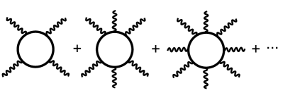
Figure 1: Fig. 1. Diagrammatic expansion of the one-loop EHL

in the diagrams above the external photons have all energies $\hbar\omega<<mc^{2}$, since a constant field may only create zero energy photons. The main concern of this work is to present a new group theoretical approach to calculate multiloop corrections in the weak field limit to the EHL, in particular we demonstrate how this is done at the three-loop level.

The motivation behind this calculation is to investigate the asymptotic behaviour of the multi-loop EHL in the weak-field regime to probe a non-perturbative conjecture that presently stands based on previous results obtained by Borel summation methods [8] and worldline instanton techniques [11]. The conjecture in question is an asymptotic relation between the imaginary part of the all-order EHL and the one-loop EHL in a weak purely electric field

$$\sum_{\ell=0}^{\infty}\mbox{Im}\mathcal{L}^{(\ell)}(E)~{}\sim^{\!\!\!\!\!\!\!\!E\to 0}\mbox{Im}\mathcal{L}^{(1)}(E)e^{\alpha\pi}$$ (1)

Where $\mathcal{L}^{(\ell)}(E)$ is the $\ell$-loop correction to the EHL. This prediction, which we shall call the exponential conjecture is grounded on the Affleck-Alvarez-Manton formula [11] and closely linked to P. Cvitanovic’s conjecture on the convergence of the quenched series of QED [16].

For the case at hand we chose to investigate this prediction for the EHL of a constant field in the toy model 1+1 QED, this choice was motivated by the result of Krasnansky [12], who showed that even at $\ell=2$ the EHL for a constant field in 1+1 scalar QED has essentially the same structure as that of 3+1 scalar QED, and the realisation that self-dual fields provide substantial computational simplifications [13, 14, 15], our goal being to compare a self-dual field in 3+1 QED against a constant field in 1+1 QED.

The exponential conjecture can be extended to dimension $D=2$, in scalar QED this was done in [9, 10]

$$\sum_{\ell=0}^{\infty}\mbox{Im}\mathcal{L}^{(\ell)}(E)~{}\sim^{\!\!\!\!\!\!\!\!E\to 0}\frac{eE}{4\pi}e^{-\frac{m^{2}\pi}{eE}+\tilde{\alpha}\pi^{2}\kappa^{2}}$$ (2)

where $\tilde{\alpha}=\frac{2e^{2}}{\pi m^{2}}$ is the fine structure constant in two dimensions and $\kappa=m^{2}/2eE$. In the weak field regime the $\ell$-loop EHL for $D=2$ has the Taylor series expansion

$$\mathcal{L}_{2D}^{(\ell)}=\frac{m^{2}}{2\pi}\sum_{n=1}^{\infty}(-1)^{\ell-1}c^{(\ell)}_{2D}(n)(i\kappa)^{-2n}$$ (3)

Contrary to $D=4$ QED in $D=2$ the asymptotic growth of the coefficients $c^{(\ell)}_{2D}(n)$ increases with $\ell$, this may be related to the fact that in two dimensions the Coulomb potential is confining. Borel analysis of (2) leads to the following condition on the coefficients

$$\lim_{n\to\infty}\frac{c^{(\ell)}_{2D}(n)}{c^{(1)}_{2D}(n+\ell-1)}=\frac{(\tilde{\alpha}\pi^{2})^{\ell-1}}{(\ell-1)!}$$ (4)

This prediction was verified in [9, 10] at the level $\ell=2$. Further differences and analogies between $D=4$ and the technically far simpler $D=2$ toy model suggest pushing this calculation to the level $\ell=3$ and higher orders to learn more about the validity of the exponential conjecture. This question will be pursued fully in the upcoming work [17]. An adequate approach to carry out the computation of the expansion coefficients is thus needed, and while different approaches might work we have proposed a technique based on the discrete symmetries of each Feynman graph. For definiteness consider the EHL $\mathcal{L}^{(3)}_{2D}$, it has dominant contributions from the Feynman diagrams A and B

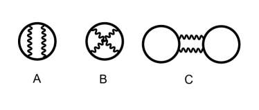
Figure 2: Fig. 2a. Dominant amplitudes in the three-loop EHL

and subdominant contributions coming from diagram C and the diagrams

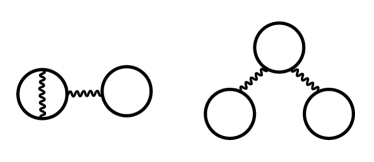
Figure 3: Fig. 2b. Subdominant amplitudes in the three-loop EHL

In these five diagrams the fermion lines represent the full propagator under the external field. Remarkably, and contrary to a long held belief, the tadpole diagrams in Fig. 2b are non-vanishing, as was first pointed out by an actual calculation done by H. Gies and F. Karbstein [7]. To exemplify the technique we shall center our efforts in calculating diagram B below, to this end we introduce the Schwinger parameters $z,z^{\prime},\bar{z},\hat{z}$:

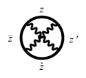
Figure 4: Fig. 3. Diagram B with dihedral symmetry $D_{4}$

the amplitude in diagram $B$ is then written as a fourfold integral over the Schwinger parameters

$$\Gamma^{(B)}= \frac{1}{32\pi^{3}}\frac{e^{3}}{f}\int_{0}^{\infty}\!\!\!\int_{0}^{\infty}\!\!\!\int_{0}^{\infty}\!\!\!\int_{0}^{\infty}dzdz^{\prime}d\hat{z}d\bar{z}\,e^{-2\kappa(z+z^{\prime}+\hat{z}+\bar{z})}$$

$$\biggl{\{}\frac{1}{\cosh^{2}z\cosh^{2}z^{\prime}\cosh^{2}\hat{z}\cosh^{2}\bar{z}}\frac{B}{A^{3}C}$$

$$-4\kappa^{2}\frac{\cosh({{z-z^{\prime}+\hat{z}-\bar{z}}})}{\cosh z\cosh z^{\prime}\cosh\hat{z}\cosh\bar{z}}\Bigl{[}\frac{1}{A}-\frac{C}{G^{2}}\ln\Bigl{(}1+\frac{G^{2}}{AC}\Bigr{)}\Bigr{]}\biggr{\}}$$

where we used the following shorthands

$$A = \tanh z+\tanh z^{\prime}+\tanh\hat{z}+\tanh\bar{z},$$

$$B = (\tanh^{2}z+\tanh^{2}\hat{z})(\tanh z^{\prime}+\tanh\bar{z})+$$

$$(\tanh^{2}z^{\prime}+\tanh^{2}\bar{z})(\tanh z+\tanh\hat{z}),$$

$$C = \tanh z\tanh z^{\prime}\tanh\hat{z}+\tanh z\tanh z^{\prime}\tanh\bar{z}+$$

$$\tanh z\tanh\hat{z}\tanh\bar{z}+\tanh z^{\prime}\tanh\hat{z}\tanh\bar{z},$$

$$G = \tanh z\tanh\hat{z}-\tanh z^{\prime}\tanh\bar{z}$$

a direct attempt to carry out the integrations, even after Taylor expansion has been carried out, is hopeless due to spurious singularities in the logarithm that symbolic computation software as MATHEMATICA fails to handle. This problem calls for another approach able to manage these singularities, and one such approach will be outlined in what follows.

2 Group Theory in QFT

As we have seen Diagram B is difficult to compute. The main idea to obtain the weak field limit of this diagram is to use its high degree of symmetry and to organise the expansion by mean of group theory. In fact it can directly observed that diagram $B$ is invariant under the following transformations ($z=\rho w,z^{\prime}=\rho w^{\prime},\hat{z}=\rho\hat{w},\bar{z}=\rho\bar{w},\rho=\frac{ef}{m^{2}}$) :

$$\begin{array}[]{lclc}g_{1}:&w&\leftrightarrow&\hat{w}\ ,\\ g_{2}:&w^{\prime}&\leftrightarrow&\bar{w}\ ,\\ g_{3}:&(w,\hat{w})&\leftrightarrow&(w^{\prime},\bar{w})\ .\end{array}$$ (8)

The group generated by the three transformations above is eight-dimensional, non-abelian and corresponds to the Dihedral group $D_{4}$. In fact, the procedure we will present below is quite general and could be applied for Feynman diagrams presenting a high degree of symmetry in any QFT.

2.1 Polynomial invariants for finite group

In this subsection we briefly present the method. Consider now $G$ a finite group and let $\rho(G)=\Gamma\subset GL(n,\mathbb{R})$ be an $n-$dimensional real representation of $G$. The representation $\Gamma$ can be reducible or irreducible. Note also that $\Gamma$ is assumed to be a real representation, but the method is equally valid for complex or pseudo-real representations. Noting $\mathbb{R}^{n}$ the carrier space of the representation $\Gamma$, for any $X=(x_{1},\cdots,x_{n})^{t}\in\mathbb{R}^{n}$ the representation $\rho$ induces naturally an action onto the set of polynomials $\mathbb{R}[x_{1},\cdots,x_{n}]$ with $n$ variables as follows

$$g.P(X)\equiv P(g.X)\ ,$$

for any $g\in\Gamma$ with $g.X$ the natural action of $g$ on $X=(x_{1},\cdots,x_{n})^{t}\in\mathbb{R}^{n}$.

Definition 2.1

Let $P\in\mathbb{R}[x_{1},\cdots,x_{n}]$, the polynomial $P$ is said to be invariant iff

$$\forall g\in\Gamma\ \ g\cdot P(X)=P(X)\ .$$

The set of invariant polynomial is denoted

$$\mathbb{R}[x_{1},\cdots,x_{n}]^{\Gamma}=\Big{\{}I\in\mathbb{R}[x_{1},\cdots,x_{n}]\ \ \text{s.t.}\ \ g\cdot I(X)=I(X)\ \ \forall g\in\Gamma\Big{\}}\ .$$

If we perform a Taylor expansion around zero of Molien’s generating function $\Phi(t)$

$$\Phi(t)=\frac{1}{|G|}\sum\limits_{g\in\Gamma}\frac{1}{\det(1-tg)}=\sum\limits_{k=0}^{+\infty}n_{k}t^{k}\ ,$$

the coefficients $n_{k}$ precisely give the number of linearly invariant polynomial of degree $k$. Of course it is obvious that these polynomials are not algebraically independent. For instance any degree $k$ invariant polynomial $I_{k}$ gives rise to a the degree $2k$ invariant polynomial $I_{k}^{2}$. So one may naturally wonder if one can define a “basis” (in a sense to be defined) of polynomial invariants. In fact we now recall that any invariant can be expressed in terms of the so-called primitive and secondary invariants [1].

Proposition 2.2

Let $G$ be a finite group and let $\Gamma$ be an $n-$dimensional (real) representation.

1. There exists $n=\dim(\Gamma)$ algebraically invariants polynomals, $P_{1},\cdots,P_{n}$, i.e., such that the Jacobian

   $$\frac{\partial(P_{1},\cdots,P_{n})}{\partial(x_{1},\cdots,x_{n})}\neq 0$$

   called the primitive invariants. Denote $d_{k}=\deg(P_{k})$ and ${\cal R}=\mathbb{R}[P_{1},\cdots,P_{n}]$ the subalgebra of polynomial invariants generated by the primitive invariants.

2. There exists $m=d_{1}\cdots d_{n}/|G|$ secondary invariants polynomials $S_{1},\cdots,S_{m}$.

3. The set of polynomials $(P_{1},\cdots,P_{n},S_{1},\cdots,S_{m})$ is not algebraically independant and satisfy algebraic relations called syzygies.

4. The subalgebra of invariants $\mathbb{R}[x_{1},\cdots,x_{n}]^{\Gamma}$ is a free ${\cal R}-$module with basis $(S_{1},\cdots,S_{m})$. In particular this means that any invariant $I\in\mathbb{R}[x_{1},\cdots,x_{n}]^{\Gamma}$ can be uniquely written as

   $$I=\sum\limits_{i=1}^{m}f_{i}(P_{1},\cdots,P_{n})S_{i}\ ,$$ (9)

   where $f_{i}(P_{1},\cdots,P_{n}),i=1,\cdots,m$ belongs to ${\cal R}$, i.e., are polynomials in $(P_{1},\cdots,P_{n})$.

The syzygies have a natural interpretation in terms of (9). Consider for instance the secondary invariant polynomials $S_{i}$, thus $S_{i}^{2}$ is an invariant polynomial, and by Proposition 2.2 there exists $f_{i,1},\cdots,f_{i,n}\in{\cal R}$ such that

$$S_{i}^{2}-\sum\limits_{j=1}^{m}f_{i,j}(P_{1},\cdots,P_{n})S_{j}=0\ ,$$

these relations among the $P$s and the $S$s are syzygies.

In general given a finite group $G$ and a representation $\Gamma$, it is not an obvious task to identify the primary and the secondary polynomials. In fact there exist many automated ways to solve this problem. In this paper, we have used the Computer Algebra System for Polynomial Computations called SINGULAR [2].

Example 2.3

Let $\Sigma_{4}$ be the permutation group acting on four elements and let $\Gamma=\mathbb{R}^{4}$ be the four-dimensional representation. The set of symmetric polynomials of degree $d=1,\cdots,4$ is the set of primitive invariants and the only secondary invariant is $\sigma_{0}=1$. Introducing the symmetric polynomials

$$\sigma_{1} = w+\hat{w}+w^{\prime}+\bar{w}\ ,$$

$$\sigma_{2} = w\hat{w}+ww^{\prime}+w\bar{w}+\hat{w}w^{\prime}+\hat{w}\bar{w}+w^{\prime}\bar{w}\ ,$$

$$\sigma_{3} = w\hat{w}w^{\prime}+w\hat{w}\bar{w}+ww^{\prime}\bar{w}+w^{\prime}\hat{w}\bar{w}$$

$$\sigma_{4} = w\hat{w}w^{\prime}\bar{w}\ .$$

we have for any invariant polynomial

$$I(w,w^{\prime},\bar{w},\hat{w})=P(\sigma_{1},\sigma_{2},\sigma_{3},\sigma_{4})\ .$$

Example 2.4

Let $D_{4}$ be the Dihedral group and let $\Gamma=\mathbb{R}^{4}$. It is obvious that in this case not all the $\sigma$s of Example 2.3 are invariant polynomials. In this case the Molien series takes the form:

$$\Phi(t) = \frac{1}{8}\Big{(}\frac{2}{1-t^{4}}+\frac{2}{(1-t)^{3}(1+t)}+\frac{3}{(1-t^{2})^{2}}+\frac{1}{(1-t)^{4}}\Big{)}$$

$$= 1+t+3t^{2}+4t^{3}+8t^{4}+10t^{5}+16t^{6}+O(t^{7})$$

and there are e.g. four degree three invariant polynomials. Now, using SINGULAR, we obtain the primitive invariants

$$a = \sigma_{1}=w+\hat{w}+w^{\prime}+\bar{w}\ ,$$

$$\lambda = (w+\hat{w})(w^{\prime}+\bar{w})\ ,$$

$$\mu = w\hat{w}+w^{\prime}\bar{w},$$

$$d = \sigma_{4}=w\hat{w}w^{\prime}\bar{w}\ ,$$

of degree $d_{1}=1,d_{2}=d_{3}=2,d_{4}=4$ respectively. A direct computation gives

$$\frac{\partial(a,\lambda,\mu,d)}{\partial(w,w^{\prime},\hat{w},\bar{w})}=(w-w^{\prime})(w-\bar{w})(w-\hat{w})(w^{\prime}-\bar{w})(w^{\prime}-\hat{w})(\bar{w}-\hat{w})\ .$$

Thus the number of secondary invariants is

$$m=\frac{1\times 2^{2}\times 4}{8}=2\ .$$

Using SINGULAR, again the secondary invariant are given by

$$\sigma_{0}=1\ ,\quad c=\sigma_{3}=ww^{\prime}\hat{w}+ww^{\prime}\bar{w}+w\bar{w}\hat{w}+w^{\prime}\hat{w}\bar{w}\ .$$

In this case, the syzygy is

$$\lambda(\mu^{2}-4d)+a^{2}d-a\mu c\ +c^{2}\ =0\ .$$

Thus any invariant polynomial uniquely writes like

$$I(w,w^{\prime},\bar{w},\hat{w})=f(a,\lambda,\mu,d)+g(a,\lambda,\mu,d)c\ ,$$

with $f,g\in\mathbb{R}[a,\lambda,\mu,d]$.

We have considered so far the so-called invariant polynomials. It turns out that there exists another class of polynomial:

Definition 2.5

Let $P\in\mathbb{R}[x_{1},\cdots,x_{n}]$, the polynomial $P$ is said to be semi-invariant iff

$$\forall g\in G,\ \ g.P(X)=e^{i\varphi(g)}\;P(X)\ ,$$

where the phase $\varphi(g)$ depends on the element $g$. Since we are concerned with real representations we have here $e^{i\phi(g)}=\pm 1$ and $P$ is invariant up to a sign.

The consideration of semi-invariant polynomials will be in turn essential to improve our algorithm.

Method 2.6

Considering a given Feynman diagram depending on some parameters and invariant under a finite group of symmetry, then the computation of this Feynman diagram can be organised by means of the invariant polynomials (in the parameters on which the Feynman diagram depends) of $G$.

This is precisely Method 2.6 that we will use to compute diagram $B$ with some improvement involving semi-invariant polynomials.

2.2 Application to diagramm $B$

Method 2.6 is general, however in our particular case the method can be improved by the inclusion of semi-invariants. Thus, we now introduce

$$\tilde{w} = w+\hat{w}-w^{\prime}-\bar{w}$$

$$g = w\hat{w}-\bar{w}w^{\prime}$$

$$j = (w-\hat{w}-w^{\prime}+\bar{w})(w-\hat{w}+w^{\prime}-\bar{w})$$

$$j^{\prime} = (w-\hat{w})(\bar{w}-\ w^{\prime})\ ,$$

which are semi-invariant. Indeed, it can be checked easily that $\tilde{w},g$ and $j$ change sign only under the action of $g_{3}$ whereas $j^{\prime}$ changes sign under the action of $g_{1}$ and $g_{2}$. Since square or appropriate product of semi-invariants leads to invariant, we introduce a new set of invariants:

$$a = w+w^{\prime}+\hat{w}+\bar{w}$$

$$v = 2\mu+\lambda=(w+\hat{w})(w^{\prime}+\bar{w})+2w\hat{w}+2w^{\prime}\bar{w}$$

$$\tilde{w}^{2} = (w+\hat{w}-w^{\prime}-\bar{w})^{2}$$

$$j^{2} = (w-\hat{w}-w^{\prime}+\bar{w})^{2}(w-\hat{w}+w^{\prime}-\bar{w})^{2}$$

which are respectively of degree $1,2,2,4$. Since the Jacobian

$$\frac{\partial(a,v,\tilde{w}^{2},j^{2})}{\partial(w,w^{\prime},\bar{w},\hat{w})}=128jj^{\prime}\ ,$$

the set of polynomial $(a,\tilde{w}^{2},v,j^{2})$ constitute an adapted set of primary invariants. Now, the syzygy takes a more complicated form:

$${c}^{2}+\left(\frac{{a}^{3}}{8}+\frac{a{{\it\tilde{w}}}^{2}}{8}-\frac{av}{2}\right)c+{\frac{{a}^{6}}{256}}+{\frac{{a}^{4}{{\it\tilde{w}}}^{2}}{128}}-\frac{{a}^{4}v}{32}-\frac{{a}^{2}v{{\it\tilde{w}}}^{2}}{32}-{\frac{{j}^{2}{{\it\tilde{w}}}^{2}}{64}}+{\frac{{a}^{2}{{\it\tilde{w}}}^{4}}{256}}+\frac{{a}^{2}{v}^{2}}{16}=0\ .$$

This simply means that now any invariant polynomial writes

$$I(w,w^{\prime},\bar{w},\hat{w})=f(a,v,\tilde{w}^{2},j^{2})+g(a,v,\tilde{w}^{2},j^{2})c\ .$$ (10)

This new set is more adapted for our purpose as we now show. Let

$$\tilde{d}=\partial_{w}+\partial_{\hat{w}}-\partial_{w^{\prime}}-\partial_{\bar{w}}\ .$$

This operator has the property to map an invariant polynomial to a semi-invariant polynomial which picks up a sign under $g_{1}$. Moreover, it is immediate to observe that

$$\tilde{d}(a)=\tilde{d}(j)=\tilde{d}(v)=0\ \ \text{and}\ \ \tilde{d}(\tilde{w})=4\ .$$

Observing that $\tilde{d}(c)=-2g$, the method can be further improved eliminating $c$ in (10) through the relation

$$c=\frac{4a^{2}v+j^{2}-a^{4}-16g^{2}}{16a}\ ,\ \ g=\frac{a\tilde{w}-j}{4}\ .$$ (11)

The substitution of (11) in (10) gives for any invariant polynomial

$$I(w,w^{\prime},\bar{w},\hat{w})=f(a,v,\tilde{w}^{2},j^{2})+g(a,v,\tilde{w}^{2},j^{2})\frac{4a^{2}v+j^{2}-a^{4}-(a\tilde{w}-j)^{2}}{16a}=\frac{P(a,v,j,\tilde{w})}{a}\ ,$$ (12)

where now the polynomial $P$ is uniquely defined because $f$ and $g$ are unique. Moreover, $P$ depends on the invariant polynomials $(a,v)$ and on the semi-invariant polynomials $(j,\tilde{w})$. The important property of our algorithm is that all these variables but $\tilde{w}$ are in the kernel of $\tilde{d}$. Since

$$\frac{\partial(a,v,j,\tilde{w})}{\partial(w,w^{\prime},\bar{w},\hat{w})}=-32(\bar{w}-w^{\prime})(w-\hat{w})\ ,$$

we are sure that the variables $(a,v,j,\tilde{w})$ are algebraically independent. We finally define

$$h=ac+g^{2}\ ,$$

which is also in the kernel of $\tilde{d}$

We now apply the method to the second part of diagram $B$ which is the most difficult integral appearing in the whole three-loop calculation. The weak field expansion of $I_{B}$ gives

$$I_{B}^{\text{hard}} = -\rho\frac{\cosh\rho(w-w^{\prime}+\hat{w}-\bar{w})}{\cosh\rho w\cosh\rho w^{\prime}\cosh\rho\bar{w}\cosh\rho\hat{w}}\Big{[}\frac{1}{A}-\frac{C}{G^{2}}\ln(1+\frac{G^{2}}{AC})\Big{]}$$

$$= \sum\limits_{n=0}^{\infty}\beta_{n}^{\text{hard}}\rho^{2n}\ .$$

Now, $\beta_{n}$ develops using $1+\frac{g^{2}}{ac}=\frac{1}{1-\frac{g^{2}}{h}}$ as

$$\beta_{n}^{\text{hard}}=\sum\limits_{k,\ell}u_{n}^{k,\ell}(w,w^{\prime},\hat{w},\bar{w})\frac{1}{g^{k}(h-g^{2})^{\ell}}+\sum\limits_{k}v_{n}^{k}(w,w^{\prime},\hat{w},\bar{w})\frac{\ln\Bigg{(}\frac{1}{1-\frac{g^{2}}{h}}\Bigg{)}}{g^{k}}$$

Using (12), we have

$$u_{n}^{k,\ell}(w,w^{\prime},\hat{w},\bar{w}) = \frac{P_{n}^{k,\ell}(a,v,j,\tilde{w})}{a}\ ,$$

$$v_{n}^{k}(w,w^{\prime},\hat{w},\bar{w}) = \frac{P_{n}^{k}(a,v,j,\tilde{w})}{a}\ ,$$

For the lowest order of the expansion we have

$$\beta_{0}^{\rm hard} = u_{0}^{0,0}+v_{0}^{0}\ln\Bigg{(}\frac{1}{1-\frac{g^{2}}{h}}\Bigg{)}+v_{0}^{2}\frac{\ln\Bigg{(}\frac{1}{1-\frac{g^{2}}{h}}\Bigg{)}}{g^{2}}\ ,$$

$$\beta^{\rm hard}_{1} = u_{1}^{00}+u_{1}^{20}\frac{1}{g^{2}}+\ln\Big{(}1+\frac{g^{2}}{ac}\Big{)}\Bigg{\{}v_{1}^{2}\frac{1}{g^{2}}+v_{1}^{4}\frac{1}{g^{4}}\Bigg{\}}\ .$$

with

$$u_{0}^{0,0}=-\frac{1}{a}\ ,\ \ v_{0}^{0}=-\frac{1}{a}\ ,\ \ v_{0}^{2}=\frac{h}{a}\ ,$$

and

$$u_{1}^{00} = \frac{a}{6}-\frac{\tilde{w}^{2}}{2a}-\frac{c}{a^{2}}\ ,$$

$$u_{1}^{20} = -{\frac{{a}^{5}}{96}}-{\frac{{a}^{3}{{\it\tilde{w}}}^{2}}{192}}+\frac{{a}^{3}v}{16}-{\frac{{a}{{\it\tilde{w}}}^{4}}{192}}-\frac{{a}{v}^{2}}{12}+\frac{{a}{{\it\tilde{w}}}^{2}v}{48}+{\frac{{a}{j}^{2}}{192}}+{\frac{{{\it\tilde{w}}}^{2}{j}^{2}}{64a}}$$

$$+c\left(-\frac{{a}^{2}}{16}-\frac{{{\it\tilde{w}}}^{2}}{6}+\frac{v}{3}\right)\ ,$$

$$v_{1}^{2} = {\frac{5\,{a}^{5}}{768}}-{\frac{a{j}^{2}}{192}}-{\frac{{a}^{3}{{\it\tilde{w}}}^{2}}{384}}-\frac{{a}^{3}v}{32}+{\frac{a{{\it\tilde{w}}}^{4}}{768}}+\frac{a{v}^{2}}{48}+{\frac{a{{\it\tilde{w}}}^{2}v}{96}}+c\left(-{\frac{13\,{a}^{2}}{24}}+{\frac{7\,{{\it\tilde{w}}}^{2}}{24}}+\frac{5v}{6}\right)\ ,$$

$$v_{1}^{4} = {\frac{7\,{a}^{7}{{\it\tilde{w}}}^{2}}{3072}}-{\frac{7\,{a}^{7}v}{768}}+{\frac{5\,{a}^{5}{{\it\tilde{w}}}^{4}}{3072}}+{\frac{5\,{a}^{5}{v}^{2}}{192}}+{\frac{{a}^{3}{{\it\tilde{w}}}^{6}}{3072}}-\frac{{a}^{3}{v}^{3}}{48}+{\frac{av{j}^{2}{{\it\tilde{w}}}^{2}}{192}}-{\frac{{a}^{3}{{\it\tilde{w}}}^{4}v}{256}}-{\frac{{a}^{3}{j}^{2}{{\it\tilde{w}}}^{2}}{256}}$$

$$-{\frac{a{{\it\tilde{w}}}^{4}{j}^{2}}{768}}+{\frac{{a}^{3}{{\it\tilde{w}}}^{2}{v}^{2}}{64}}-{\frac{5\,{a}^{5}{{\it\tilde{w}}}^{2}v}{384}}+{\frac{{a}^{9}}{1024}}$$

$$+c\left({\frac{{a}^{6}}{64}}-\frac{{a}^{2}{{\it\tilde{w}}}^{2}v}{24}-\frac{{j}^{2}v}{24}+\frac{{a}^{2}{v}^{2}}{12}+\frac{{a}^{2}{j}^{2}}{48}+\frac{{a}^{4}{{\it\tilde{w}}}^{2}}{32}-\frac{{a}^{4}v}{12}+{\frac{{a}^{2}{{\it\tilde{w}}}^{4}}{64}}\right)\ .$$

It remains of course to make the substitution (11) for $c$. Now using partial integration upon $\tilde{d}$ we can integrate out the variable $\tilde{w}$ and finally calculate $\beta_{0}^{\rm hard}$ and $\beta_{1}^{\text{hard}}$, see [17]

$$\int_{0}^{\infty}dwdw^{\prime}d\hat{w}d\bar{w}\,\e^{-a}\beta^{\rm hard}_{0} = -\frac{13}{12}+\frac{7}{8}\zeta_{3}$$

$$\int_{0}^{\infty}dwdw^{\prime}d\hat{w}d\bar{w}\,\e^{-a}\beta_{1}^{\text{hard}} = \phantom{-}\frac{121}{64}-\frac{203}{128}\zeta_{3}\ .$$

3 Final Remarks

The method presented here has proven effective and useful in the calculation of weak field coefficients of a Feynman diagram (diagram B) but is not necessarily restricted to such regime. Indeed, although we know not of a concrete example presently it is plausible that for certain class of Feynman diagrams their exact calculation might be carried out along very similar, if not almost identical, lines. This would imply that the scope of the method is farther reaching than has been exploited here. Nevertheless we must admit the speculative nature of this assertion and await for any such examples that may emerge in future investigations.

References

References

• [1] Sturmfels B 2008 Algorithms in invariant theory 2nd edn. (Springer Berlin)
• [2] Decker W and Lossen C 2006 Computing in algebraic geometry. A quick start using SINGULAR (Springer Berlin)
• [3] Martin L, Schubert C and Villanueva Sandoval V M 2003 Nucl. Phys. B668 335 hep-th/0301022
• [4] Heisenberg W and Euler H 1936 Z. Phys. 98 714
• [5] Dittrich W and Gies H 2000 Springer Tracts Mod. Phys. 166 1
• [6] Dunne G V 2002 Cont. Adv. in QCD 478 hep-th/0207046
• [7] Gies H and Karbstein F 2017 JHEP 03 108
• [8] Dunne G V and Schubert C 2000 Nucl.Phys. B564 591
• [9] Huet I, McKeon D G C and Schubert C 2010 Quantum Field Theory Under The Influence Of External Conditions (Qfext09) (World Scientific)
• [10] Huet I, McKeon D G G and Schubert C 2010 JHEP 1012 036 hep-th/1010.5315
• [11] Affleck I K, Alvarez O and Manton N S 1982 Nucl. Phys. B197 509
• [12] Krasnansky M 2008 Int. J. Mod. Phys. A23 5201 hep-th/0607230
• [13] Dunne G V and Schubert C 2002 Phys. Lett. B526 55 hep-th/0111134
• [14] Dunne G V and Schubert C 2002 JHEP 0208 053 hep-th/0205004
• [15] Dunne G V and Schubert C 2002 JHEP 0206 042 hep-th/0205005
• [16] Cvitanovic P 1977 Nucl. Phys. B127 176
• [17] Huet I, Rausch de Traubenberg M and Schubert C In preparation