$H+1$ jet production revisited

Abstract

We revisit the next-to-next-to-leading order (NNLO) calculation of the Higgs boson$+1$ jet production process, calculated in the $m_{t}\to\infty$ effective field theory. We perform a detailed comparison of the result calculated using the jettiness slicing method, with published results obtained using subtraction methods. The results of the jettiness calculation agree with the two previous subtraction calculations at benchmark points. The performance of the jettiness slicing approach is greatly improved by adopting a definition of $1$-jettiness that accounts for the boost of the Born system. Nevertheless, the results demonstrate that power corrections in the jettiness slicing method remain significant. At large transverse momentum the effect of power corrections is much reduced, as expected.

I Introduction

Testing the properties of the Higgs boson is a central theme of the experimental program of the LHC and will continue to be so for the foreseeable future. Despite the array of probes performed so far, as yet no compelling evidence for unexpected couplings of the Higgs boson to other particles has been discovered. However, as more data is accumulated, the experiments will be able to test our understanding of the nature of the Higgs boson in interesting new ways. One such direction is through the production of a Higgs boson at non-zero transverse momentum, a process mediated primarily by a Higgs boson recoiling against one or more partons. Such events contribute significantly to the total number of Higgs boson events that can be observed. This is due to the copious radiation expected from the initial-state gluons that originate the lowest-order inclusive production process. Moreover, as the hardness of the QCD radiation increases, partons are able to resolve the nature of the loop-induced coupling and the process becomes sensitive to the particles that circulate in the loop. It is for this reason that measurements of Higgs boson production in association with QCD radiation constitute a complementary probe of the Higgs boson.

To turn such measurements into compelling information on the nature of the Higgs boson requires precision theoretical calculations with which to compare the experimental data. At fixed order the description of such events can be primarily described by the recoil of a Higgs boson against a single jet, at least in a region of transverse momentum that is hard enough to be properly described by a jet. In order to achieve a suitable precision, and a sufficiently small dependence on the unphysical renormalization and factorization scales that enter the calculation, it is necessary to perform computations up to next-to-next-to-leading order (NNLO). Over the last five years such predictions have become available thanks to independent calculations from a number of groups Boughezal et al. (2013); Chen et al. (2015); Boughezal et al. (2015a, b); Caola et al. (2015); Chen et al. (2016). Beyond this, further steps have been taken to also account for the effect of the resummation of next-to-next-to-next-to-leading logarithms (N³LL) to enable a better description at small transverse momenta Chen et al. (2019); Bizon et al. (2018).

The availability of multiple calculations of Higgs+jet production at NNLO is important for a number of reasons. First of all, the calculations have been performed with a variety of different methods for handling soft and collinear divergences in real radiation contributions. The appearance of such divergences leads to considerable complication in the calculations and, depending on the details of the method, handling them could expose the calculations to issues of numerical precision or systematic flaws in the methods. Second, to the extent that independent calculations arrive at the same answer, additional confidence in the theoretical calculations and methodologies is gained. To understand these issues it is important to benchmark the calculations appropriately and perform detailed studies of any apparent disagreement. For the case at hand, a first comparison of results between the calculations was performed in the context of studies for the LHC Higgs Cross Section Working Group Yellow Report (“YR4”) de Florian et al. (2016). A comprehensive comparison was then performed by the NNLOJET group Chen et al. (2016) that found agreement with the results of Refs. Boughezal et al. (2015a); Caola et al. (2015) but was unable to confirm the results published in Ref. Boughezal et al. (2015b). The latter result was obtained using the $N$-jettiness method Boughezal et al. (2015c); Gaunt et al. (2015), that relies on a factorization theorem in Soft-Collinear Effective Theory (SCET) in order to compute a class of unresolved contributions. Therefore the resulting calculation closely resembles a traditional slicing approach to higher-order corrections and is thus sensitive to the value of a resolution parameter through the effect of power corrections to the factorization formula. To understand whether or not the difference could be attributed to such effects, for instance as suggested in Ref. Moult et al. (2017), and to understand the effectiveness of the $N$-jettiness method more generally, requires a detailed reappraisal of the calculation. This paper aims to shed light on these issues through our own implementation of the NNLO corrections to Higgs+jet production using the $N$-jettiness method.

The outline of the paper is as follows. In Section II we describe the calculation and the various checks that have been performed on the ingredients. A detailed comparison of results obtained using our calculation, and those of NNLOJET Chen et al. (2015, 2016); Bizon et al. (2018), follows in Section III. We then compare results, under a different set of cuts, with those of Ref. Boughezal et al. (2015a) in Section IV. In Section V we perform a study of the effectiveness of our calculation in the boosted region and we conclude in Section VI.

II Calculation

Our $N$-jettiness calculation of Higgs+jet production is embedded in the MCFM code Campbell et al. (2011, 2015), with many ingredients in common with previous NNLO calculations of color-singlet production Boughezal et al. (2017a) and inclusive photon and photon+jet processes Campbell et al. (2017a, b). In particular, all calculations share process-independent beam Gaunt et al. (2014a, b) and jet Becher and Neubert (2006); Becher and Bell (2011) functions. We use the soft function calculation of Ref. Campbell et al. (2018), which is in good agreement with two other evaluations of the same quantity Boughezal et al. (2015d); Bell et al. (2018). The remaining ingredient in the SCET factorization theorem for the below-cut contribution is the hard function, which we implement using the procedure of Ref. Becher et al. (2014) to obtain the result up to 2-loop order using the helicity amplitudes of Ref. Gehrmann et al. (2012). The resulting hard function has been cross-checked against the result at a fixed kinematic point that is also given in Ref. Becher et al. (2014).

The remaining ingredient in the $N$-jettiness approach is the NLO calculation of the $H+2$ jet process. However, instead of applying the usual jet cuts, only a single jet is required and additional parton configurations must pass a cut on $1$-jettiness. This quantity is defined by,

$${\mathcal{T}}_{1}=\sum_{m}\min_{i}\left\{\frac{2p_{i}\cdot q_{m}}{P_{i}}\right\}\,,$$ (1)

where the momenta $p_{i}$ are those of the partons in the initial beam and the (hardest) jet that is present in the event, and the sum runs over the momenta of all partons, $q_{m}$. A number of choices are possible for the normalization factors, $P_{i}$. In this paper we will always use the choice $P_{i}=2E_{i}$, resulting in a so-called geometric measure Jouttenus et al. (2011, 2013). However, we will define ${\mathcal{T}}_{1}$ both in the hadronic center-of-mass frame (as in previous $1$-jettiness calculations performed using MCFM Boughezal et al. (2016); Campbell et al. (2016a, b); Boughezal et al. (2017a); Campbell et al. (2017a, b)) as well as in a boosted frame in which the system consisting of the Higgs boson and the jet is at rest. As explained in, for instance, Refs. Gaunt et al. (2015); Moult et al. (2017), this is a more natural definition that should be less sensitive to power corrections at large rapidities.

Since the $H+2$ jet NLO calculation is used in a slightly different way than normal it should therefore be scrutinized in detail. In order to validate the helicity amplitudes used in our calculation we have performed a cross-check of all matrix elements, contributing to both virtual and real contributions, against those obtained using Madgraph5_aMC@NLO Alwall et al. (2014) and found complete agreement. To validate the proper treatment of all singularities we have performed extensive checks of the subtraction terms in each singular limit. We have also limited the extent of all dipole subtractions using the introduction of “$\alpha$ parameters” Nagy and Trocsanyi (1999) to test whether counter-terms have been included consistently throughout the calculation.

Up to now, $\alpha$-independence had typically only been checked for the total cross-section, usually varying all parameters at the same time. This hides potential deviations in sub-leading channels and can mask mismatches in color orderings since, for example, in some channels color orderings do not matter once final-initial and final-final dipoles are summed over. In order to provide a more stringent check on the calculation we computed the $\alpha$-dependence for each partonic initial state and also for each possible $\alpha$ parameter individually. These checks revealed a small inconsistency in the subtraction of singularities in the $q\bar{q}\to Hggg$ channel, and an even smaller discrepancy in $qg\to Hqq\bar{q}$ (identical-quark) contributions. Together, these effects resulted in $\alpha$-dependence at a very small level in the total cross-section that had not been detected previously.

To illustrate the level of $\alpha$-independence in the code used for the present calculation we will show the results of cross-checks performed using the following setup:

$${\rm LHC},~{}\sqrt{s}=13~{}{\rm TeV},\qquad \mu_{R}=\mu_{F}=m_{H}=125~{}{\rm GeV},$$

$$p_{T}^{\rm jet}>20~{}{\rm GeV},\qquad \Delta R=0.4$$ (2)

Jets are clustered according to the anti-$k_{T}$ algorithm and, as indicated above, no explicit cut on their rapidities is applied. The results are shown in Figure 1, which indicates the deviation from the default ($\alpha_{II}=\alpha_{IF}=\alpha_{FI}=\alpha_{FF}=1$) when each of the dipole parameters is set to $10^{-2}$. The deviation is measured by,

$$\epsilon^{ab}=\frac{\sigma(\alpha_{ab}=1)-\sigma(\alpha_{ab}=0.01)}{\sigma(\alpha_{ab}=1)}\,.$$ (3)

Note that, when going between these two values of $\alpha$, the virtual and real contributions each individually change by an amount that often far exceeds the total cross-section itself so that the check is a rather stringent one. The results in Figure 1 show that the cross-section is independent of the choice of $\alpha$ parameters, over a wide range, to within the Monte Carlo statistics indicated for each channel. This corresponds to a check at the $0.1\%$ level or better for all channels except $\bar{q}\bar{q}$, where the size of the cross-section is so small that the check is slightly less strict, at the $0.3\%$ level. Since, in general, the calculation is more efficient for $\alpha<1$ we choose to set $\alpha_{II}=\alpha_{IF}=\alpha_{FI}=\alpha_{FF}=0.01$ to obtain all the results presented hereafter.

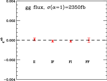
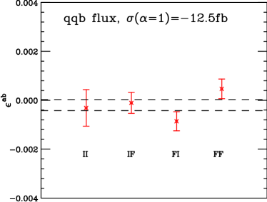
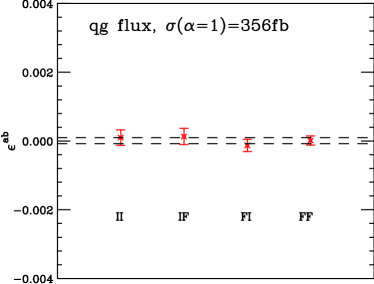
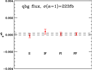
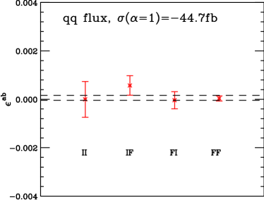
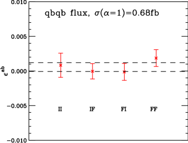
Figure 1: The dependence of the $H+2j$ cross-section on the $\alpha$ parameters, for each of the different partonic fluxes. The points represent the deviation from the default ($\alpha_{II}=\alpha_{IF}=\alpha_{FI}=\alpha_{FF}=1$) when the labelled parameter is set to $10^{-2}$. The cross-sections in this channel, obtained using the default parameters, are indicated in the plots. The dashed lines represent the uncertainty on a fit of the results to a constant, indicating excellent agreement with zero at the level of Monte Carlo statistics.

Beyond the issues discussed above, the use of the $H+2$ jet NLO process in a $1$-jettiness calculation requires a number of small further refinements. First, the evaluation of the real corrections probes partonic configurations that can become highly singular, particularly for very small values of the $1$-jettiness cut. This means that special attention must be paid to generating phase-space points in this region. Moreover, at NLO it is typical to implement a technical cut in order to remove extreme phase-space configurations in which the real emission matrix element and subtraction counter-terms should exactly cancel, but for which numerical stability can be an issue. In the NNLO calculation it is important to ensure that any such cut does not impact the result, which typically requires the cuts to be made at smaller values than in a typical NLO calculation. We have performed detailed checks to ensure that, with the technical cuts that we have used, points that are removed do not alter our results. Finally, the NLO code must be modified trivially in order to properly account for all higher-order corrections to the Wilson coefficient that couples the Higgs field to two gluons in the effective field theory Dawson (1991); Chetyrkin et al. (1997).

III Comparison with NNLOJET

We now turn to a detailed comparison with the NNLO results provided by NNLOJET Chen et al. (2015, 2016); Bizon et al. (2018), employing the setup that was used for the YR4 comparison de Florian et al. (2016). These are summarized here:

$${\rm LHC},~{}\sqrt{s}=13~{}{\rm TeV}, \quad\mu_{R}=\mu_{F}=m_{H}=125~{}{\rm GeV},$$

$$p_{T}^{\rm jet}>30~{}{\rm GeV}, \quad{\rm anti-}k_{T}~{}{\rm algorithm},~{}\Delta R=0.4$$ (4)

$${\rm PDF~{}set:} \quad{\tt PDF4LHC15\_nnlo\_30}$$

Note that this choice of PDF set is used to obtain results both at NLO and NNLO. By inspecting these cuts one might already anticipate a potential disadvantage to using the jettiness slicing method for the calculation of NNLO corrections. This is because neither the jet nor the Higgs boson is required to satisfy any rapidity constraint, leading to contributions to the cross-section from events with high-rapidity particles. These types of event have already been identified as being subject to power corrections that are large Ebert et al. (2018).

Up to NNLO in QCD, the cross-section for this process can be written as,

$$\sigma_{NNLO}=\sigma_{LO}+\delta\sigma_{NLO}+\delta\sigma_{NNLO},$$ (5)

where $\sigma_{LO}$, $\delta\sigma_{NLO}$ and $\delta\sigma_{NNLO}$ contain, respectively, only contributions of order $\alpha_{s}^{3}$, $\alpha_{s}^{4}$ and $\alpha_{s}^{5}$. The NLO cross-section, $\sigma_{NLO}$, is defined similarly by omitting the final term. In the sections that follow it is useful to compare calculations of both the higher-order coefficients $\delta\sigma_{NLO}$ and $\delta\sigma_{NNLO}$ as well as the full cross-sections at each order, $\sigma_{NLO}$ and $\sigma_{NNLO}$.

III.1 Comparison of NLO calculation

We have first cross-checked the implementation of the NLO calculation, using dipole subtraction, by comparing with the corresponding computation in NNLOJET. As shown in Table 1, we have found complete agreement between the codes at the per-mille level.

NLO calculation	$gg$	$qg$	$\bar{q}g$	$q\bar{q}$	$qq$	$\bar{q}\bar{q}$
NNLOJET	$4962\pm 3$	$546.6\pm 0.6$	$231.5\pm 0.2$	$-14.61\pm 0.03$	$-34.01\pm 0.13$	$-6.739\pm 0.008$
MCFM	$4960\pm 2$	$546.3\pm 0.4$	$231.1\pm 0.1$	$-14.62\pm 0.04$	$-33.94\pm 0.08$	$-6.731\pm 0.011$

Table 1: The NLO contribution $\delta_{NLO}$, defined in Eq. 5, broken down into individual partonic channels, as computed by NNLOJET and MCFM (dipole subtraction). Cross-sections are shown in femtobarns.

We now turn to the $1$-jettiness calculation and inspect the $\tau\textsubscript{cut}$ dependence of each partonic channel, using a value of $\tau\textsubscript{cut}$ that depends dynamically on the kinematics of each event. Specifically, we set

$$\tau\textsubscript{cut}=\epsilon\times\sqrt{m_{H}^{2}+\left(p_{T}^{j_{1}}\right)^{2}}$$ (6)

with $2\times 10^{-5}\leq\epsilon\leq 5\times 10^{-4}$. For the sake of comparison it is possible to convert these values of $\tau\textsubscript{cut}$ to a definite scale by using $p_{T}^{j_{1}}\to p_{T,\text{min}}^{j_{1}}$. In this way, these values of $\epsilon$ approximately correspond to fixed values of $\tau\textsubscript{cut}$ in the range $0.0025$ – $0.06$ GeV, although the correspondence is not exact due to contributions to the cross-section at higher jet transverse momentum. We note in passing that almost the entire range of $\tau\textsubscript{cut}$ studied here is significantly below the one studied in the previous calculation of $H+$jet production using jettiness slicing Boughezal et al. (2015b).

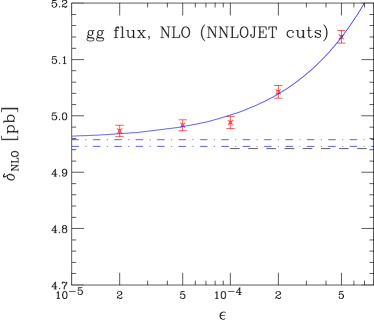
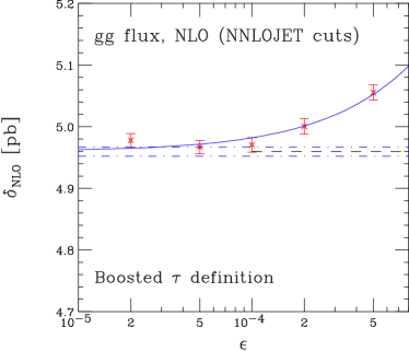
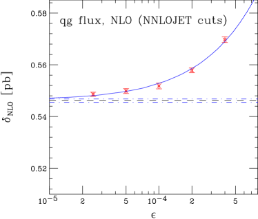
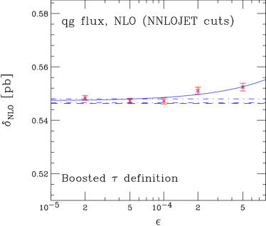
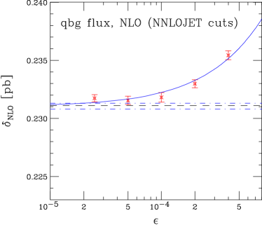
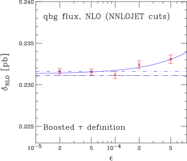
Figure 2: $\tau$-dependence of NLO coefficients for the $gg$, $qg$ and $\bar{q}g$ partonic channels, in the NNLOJET setup. The plots on the left show the result when ${\mathcal{T}}_{1}$ is computed in the hadronic c.o.m. and the ones on the right indicate the corresponding result when evaluating this quantity in the boosted frame. The (blue) solid lines correspond to the fit form in Eq. (7), with the dot-dashed lines representing the errors on the asymptotic value of the fit. The exact results, computed in MCFM using dipole subtraction, are shown as the black dashed lines.

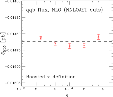
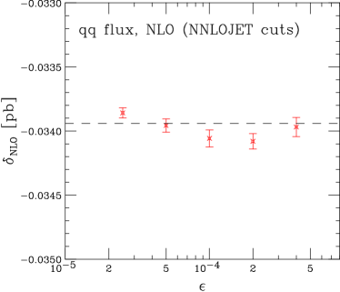
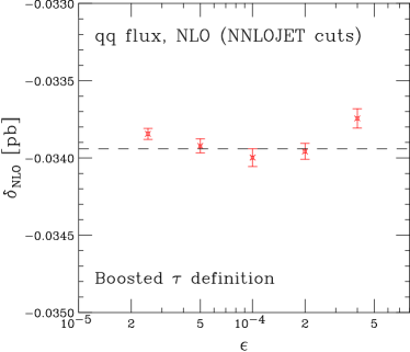
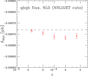
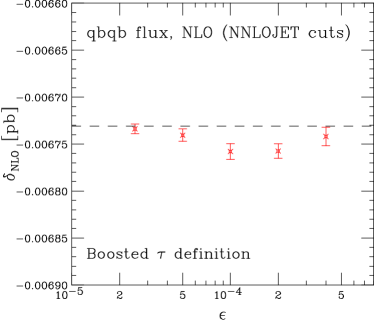
Figure 3: $\tau$-dependence of NLO coefficients for the $q\bar{q}$, $qq$ and $\bar{q}\bar{q}$ partonic channels, in the NNLOJET setup. The plots on the left show the result when ${\mathcal{T}}_{1}$ is computed in the hadronic c.o.m. and the ones on the right indicate the corresponding result when evaluating this quantity in the boosted frame. The exact results, computed in MCFM using dipole subtraction, are shown as the black dashed lines.

As a first check of the sensitivity of this process to power corrections, we examine the $\tau\textsubscript{cut}$ dependence of the NLO calculation in each of the three main partonic channels – $gg$, $qg$ and $\bar{q}g$. The results are shown in Fig. 2, for both definitions of ${\mathcal{T}}_{1}$, in the hadronic center-of-mass frame (left) and after the boost to the rest frame of the Higgs boson+jet system (right). We see that, in both cases, the jettiness result for the NLO coefficient in each channel approaches the known NLO result computed using dipole subtraction as $\tau\textsubscript{cut}\to 0$. However we also observe that, as expected, this approach is much less steep when using the boosted definition of ${\mathcal{T}}_{1}$. In order to quantify the $\tau\textsubscript{cut}$-dependence we have performed a fit to the data points using the expected behavior of the power corrections. This is prescribed by the leading singularities at this order and takes the form,

$$\delta_{NLO}^{\{gg,qg,\bar{q}g\}}(\epsilon)=\delta_{NLO}^{fit}+c_{0}\,\epsilon\log(\epsilon)+\ldots$$ (7)

These fits, shown as solid lines in Fig. 2, describe the $\tau\textsubscript{cut}$-dependence extremely well. Corresponding results for the subleading channels – $q\bar{q}$, $qq$ and $\bar{q}\bar{q}$ – are shown in Fig. 3. Again we observe excellent agreement with the exact calculation. However, from this figure it is obvious that the power corrections in these channels are tiny, with agreement between the two calculations at the per-mille level for essentially the entire range of $\tau\textsubscript{cut}$ values studied here. The reason for this is clear in the case of the $qq$ and $\bar{q}\bar{q}$ channels since they enter for the first time at this order and only contain collinear singularities. Moreover, for the $q\bar{q}$ channel the dominant contribution comes not from $s$-channel diagrams that are present at LO, but from $t$-channel scattering diagrams that only enter at NLO and have a similar singularity structure as those for $qq$ and $\bar{q}\bar{q}$. Since the effect of power corrections is so small we see essentially no gain in using the boosted definition of ${\mathcal{T}}_{1}$.

Since the boosted definition performs better, it is clear that we should use it for assessing the performance of the jettiness calculation. In order to summarize our findings we will compare with the exact NLO result, for two cases. In the first we simply use $\epsilon=5\times 10^{-5}$, while in the second we define $\delta_{NLO}^{fit}$ as the asymptotic fit value indicated in Eq. (7) for the leading channels and simply use $\epsilon=2.5\times 10^{-5}$ for the subleading channels. This comparison is shown in Table 2. We conclude that either choice reproduces the exact result at the $0.15\%$ level or better.

Calculation	$gg$	$qg$	$\bar{q}g$	$q\bar{q}$	$qq$	$\bar{q}\bar{q}$	total
$\epsilon=5\times 10^{-5}$	$4967\pm 11$	$547.3\pm 1.0$	$231.5\pm 0.4$	$-14.65\pm 0.03$	$-33.92\pm 0.05$	$-6.74\pm 0.01$	$6455\pm 19$
$\delta_{NLO}^{fit}$	$4960\pm 8$	$547.3\pm 0.7$	$231.3\pm 0.3$	$-14.57\pm 0.03$	$-33.84\pm 0.04$	$-6.73\pm 0.01$	$6447\pm 9$
Exact	$4960\pm 2$	$546.3\pm 0.4$	$231.1\pm 0.1$	$-14.62\pm 0.04$	$-33.94\pm 0.08$	$-6.73\pm 0.01$	$6445\pm 3$

Table 2: Comparison between NLO coefficients computed by MCFM, both exactly (using dipole subtraction) and by jettiness slicing (boosted definition of ${\mathcal{T}}_{1}$). Results are shown for $\epsilon=5\times 10^{-5}$ in the definition of $\tau\textsubscript{cut}$ and for a combination of fit values ($gg$, $qg$, $\bar{q}g$) and results for $\epsilon=2.5\times 10^{-5}$ ($q\bar{q}$, $qq$, $\bar{q}\bar{q}$), denoted by $\delta_{NLO}^{fit}$. Note that the total column includes a factor of two for channels that are not beam-symmetric.

III.2 Comparison of NNLO calculation

We now turn to an examination of the NNLO calculation, for which we perform a similar $\tau\textsubscript{cut}$-dependence study. As before, we first inspect the performance of the calculation in the leading partonic channels that are subject to the largest power corrections, using both versions of ${\mathcal{T}}_{1}$. The results are shown in Fig. 4, which indicates again that using the boosted definition of ${\mathcal{T}}_{1}$ results in a less dramatic approach to the asymptotic result. In contrast to the case at NLO, but as anticipated from the stronger power corrections that are present at this order, the dependence on $\tau\textsubscript{cut}$ is quite pronounced. The region in which the power corrections are under control is much reduced, even when using the boosted definition of ${\mathcal{T}}_{1}$. The results only begin to become independent of $\tau\textsubscript{cut}$, at around the $5\%$ level, for $\epsilon=10^{-4}$ or smaller. The figures also indicates the results of a fit to the data using the expected form of the power corrections at this order, which takes the form,

$$\delta_{NNLO}^{\{gg,qg,\bar{q}g\}}(\epsilon)=\delta_{NNLO}^{fit}+c_{0}\,\epsilon\log^{3}(\epsilon)+\ldots$$ (8)

This leading behavior is sufficient for the boosted definition but we observe that for ${\mathcal{T}}_{1}$ defined in the hadronic c.o.m. it may be more appropriate to include an additional subleading $\epsilon\log^{2}(\epsilon)$ term. Since the boosted definition is clearly superior, and well-described by the leading coefficient alone, we do not investigate this further. For both definitions we see that the fit value is in very good agreement with the NNLOJET result.

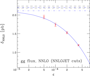
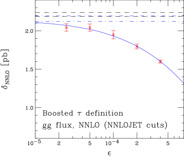
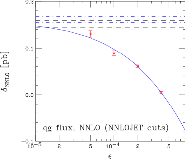
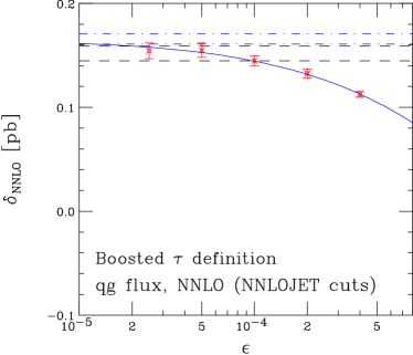
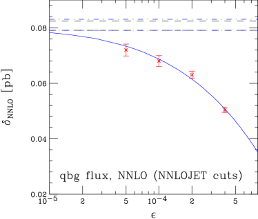
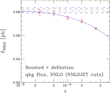
Figure 4: $\tau$-dependence of NNLO coefficients for the $gg$, $qg$ and $\bar{q}g$ partonic channels, in the NNLOJET setup. The plots on the left show the result when ${\mathcal{T}}_{1}$ is computed in the hadronic c.o.m. and the ones on the right indicate the corresponding result when evaluating this quantity in the boosted frame. The (blue) solid lines correspond to the fit form in Eq. (8), with the dot-dashed lines representing the errors on the asymptotic value of the fit. The NNLOJET result, including its associated uncertainty, is shown as the band enclosed by the black dashed lines.

A similar study of the subleading channels is shown in Fig. 5, although in this case we choose to show only the results obtained using the boosted definition of ${\mathcal{T}}_{1}$ since it is clear that the power corrections are small. In all cases there is very little dependence on $\tau\textsubscript{cut}$ and the resulting NNLO corrections are in good agreement with those from NNLOJET, apart from the $q\bar{q}$ channel that is slightly outside the error estimate. However, we note that the NNLOJET calculation with which we compare did not isolate individual channels and is therefore heavily focussed on the dominant $gg$ and $qg$ channels. As explained in Ref. Chen et al. (2019), these subleading channels are more sensitive to numerical fluctuations at larger values of $x$, which may explain the relatively poorer agreement observed in Fig. 5. For the $1$-jettiness calculation in MCFM we have indicated a fit to the power corrections using a form that reflects their weaker role in these channels,

$$\delta_{NNLO}^{\{q\bar{q},qq,\bar{q}\bar{q}\}}(\epsilon)=\delta_{NNLO}^{fit}+c_{0}\,\epsilon\log(\epsilon)+\ldots$$ (9)

However we note that, although the $\tau\textsubscript{cut}$ dependence is milder for the subleading channels, the $\tau\textsubscript{cut}$ dependence of the total NNLO correction — and hence the effectiveness of this method — is governed by the behavior of the leading channels.

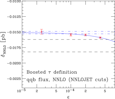
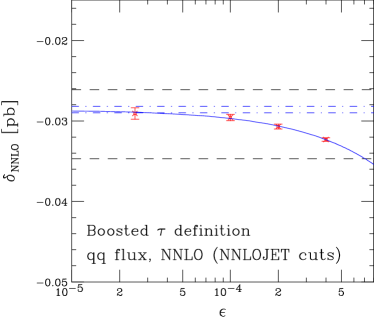
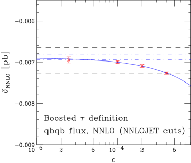
Figure 5: $\tau$-dependence of NNLO coefficients for the $q\bar{q}$, $qq$ and $\bar{q}\bar{q}$ partonic channels, in the NNLOJET setup, using ${\mathcal{T}}_{1}$ evaluated in the boosted frame. The (blue) solid lines correspond to the fit form in Eq. (9), with the dot-dashed lines representing the errors on the asymptotic value of the fit. The NNLOJET result, including its associated uncertainty, is shown as the band enclosed by the black dashed lines.

The final comparison between MCFM and NNLOJET, including also the results from the fits, is shown in Table 3. Note that we also include, separately and for reference, the contribution from the Wilson coefficient correction that enters at NNLO. Note that this contribution may be computed exactly (without any $\tau\textsubscript{cut}$ dependence) since it is simply related to the NLO coefficient. Since the $\tau\textsubscript{cut}$-dependence is stronger at NNLO we use $\epsilon=2.5\times 10^{-5}$ as the point at which we compare our non-fitted results. We conclude that this value reproduces the NNLOJET result to within about $5-10\%$ for all channels, with a significant improvement in the agreement – especially for the leading $gg$ channel – when using the fitted asymptotic result.

Calculation	$gg$	$qg$	$\bar{q}g$	$q\bar{q}$	$qq$	$\bar{q}\bar{q}$	total
NNLO Wilson	$879\pm 2$	$93.4\pm 0.4$	$40.2\pm 0.2$	$-3.0\pm 0.0$	$-6.61\pm 0.0$	$-1.33\pm 0.01$	$1132\pm 3$
$\epsilon=2.5\times 10^{-5}$	$2043\pm 49$	$154\pm 7$	$79.5\pm 2.3$	$-15.0\pm 0.4$	$-29.1\pm 0.7$	$-6.95\pm 0.07$	$2444\pm 69$
$\delta_{NNLO}^{fit}$	$2159\pm 37$	$166\pm 5$	$82.2\pm 1.5$	$-15.1\pm 0.2$	$-28.6\pm 0.4$	$-6.90\pm 0.04$	$2590\pm 51$
NNLOJET	$2213\pm 25$	$152\pm 7$	$80.8\pm 1.7$	$-17.2\pm 1.0$	$-30.6\pm 4.1$	$-6.97\pm 0.32$	$2607\pm 49$

Table 3: Comparison between MCFM and NNLOJET results for the NNLO coefficient $\delta_{NNLO}$, defined in Eq. 5, in the YR4 setup detailed in the text. We also show separately the NNLO Wilson coefficient contribution to $\delta_{NNLO}$. Results are shown for the boosted definition of ${\mathcal{T}}_{1}$, for $\epsilon=2.5\times 10^{-5}$ and also for the fit values ($\delta_{NNLO}^{fit}$). Note that the total column includes a factor of two for channels that are not beam-symmetric and uncertainties on individual channels are combined linearly in the total.

It is useful to perform a cross-check that also tests the scale-dependence of the full result. For this we employ a simple 2-point variation in which both renormalization and factorization scales vary by a factor of two together about the central choice. At the preceding orders in perturbation theory we find,

$$\sigma_{LO}(\mathrm{MCFM})=7.66^{+2.92}_{-1.98}\,\text{pb}\,,$$ (10)

and,

$$\sigma_{NLO}(\mathrm{MCFM})=14.12^{+2.83}_{-2.45}\,\text{pb}\,,$$ (11)

which are in complete agreement with the corresponding results from NNLOJET. At NNLO we first examine the non-fitted result and find,

$$\sigma_{NNLO}(\mathrm{MCFM},\epsilon=2.5\times 10^{-5})=16.56\pm 0.07\,^{+1.03}_{-1.52}\,\text{pb}\,,$$ (12)

where the error from the Monte Carlo calculation is shown first, and the scale uncertainty is indicated by the sub- and super-scripts. This is to be compared with the corresponding result from NNLOJET,

$$\sigma_{NNLO}(\mathrm{NNLOJET})=16.73\pm 0.05\,^{+1.00}_{-1.51}\,\text{pb}\,.$$ (13)

We see that, since the NNLO corrections are so large, the difference between the total NNLO result computed with NNLOJET and MCFM is at the $1\%$ level and outside the (combined) $0.5\%$ Monte Carlo errors. Although this difference does lie well within the residual NNLO scale uncertainty, the fact that agreement is only at the percent level potentially limits the range and power of the phenomenology that may be performed with this result. However, we note that the use of the asymptotic fits for the central result yields excellent agreement,

$$\sigma_{NNLO}(\mathrm{MCFM,fit})=16.71\pm 0.05\,^{+1.03}_{-1.52}\,\text{pb}\,.$$ (14)

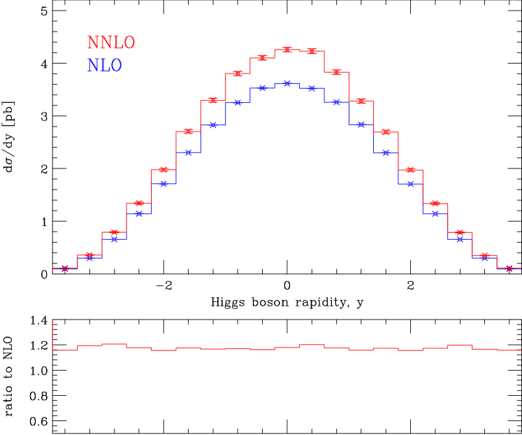
Figure 6: The rapidity distribution of the Higgs boson computed at NLO and NNLO using MCFM, in the NNLOJET setup. The NNLO coefficient is calculated using $\epsilon=2.5\times 10^{-5}$ in the boosted definition of ${\mathcal{T}}_{1}$. The lower panel shows the ratio of the NNLO and NLO results.

We conclude this section by examining the calculation of a more differential quantity, the rapidity spectrum of the Higgs boson. We show the NLO and NNLO predictions for this observable in Fig. 6, where the NNLO coefficient is calculated using $\epsilon=2.5\times 10^{-5}$ in the boosted definition of ${\mathcal{T}}_{1}$. The effect of the NNLO corrections is approximately constant in rapidity, with an overall impact that is in excellent agreement with NNLOJET (c.f. Fig. 24 of Ref. de Florian et al. (2016)).

IV Comparison with BCMPS

We now turn to a detailed comparison with results obtained using the calculation of Boughezal, Caola, Melnikov, Petriello and Schulze (BCMPS) Boughezal et al. (2015a). Apart from being a cross-check with a different calculation, this comparison provides additional insight since the setup is slightly different. The setup for the comparison is as follows:

$${\rm LHC},~{}\sqrt{s}=13~{}{\rm TeV}, \quad\mu_{R}=\mu_{F}=m_{H}=125~{}{\rm GeV},$$

$$p_{T}^{\rm jet}>20~{}{\rm GeV}, \quad{\rm anti-}k_{T}~{}{\rm algorithm},~{}\Delta R=0.4$$ (15)

$${\rm PDF~{}set:} \quad{\tt PDF4LHC15\_nnlo\_mc}$$

In addition, in the calculation of Ref. Boughezal et al. (2015a) NNLO corrections to the 4-quark channels, that first enter the calculation at NLO, are not included. The essential difference with respect to the previous calculation is the slight reduction in the jet $p_{T}$ cut (from $30$ to $20$ GeV), which one expects to render the jettiness calculation more difficult to perform since the power corrections should be larger for the same value of $\tau\textsubscript{cut}$.

As before, we examine the NNLO coefficient alone and separated into partonic channels. In this case the BCMPS calculation can be easily broken down into three contributions with which we can compare: $gg$, $qg+\bar{q}g$ and $q\bar{q}+qq+\bar{q}\bar{q}$, where factors of two to include all beam-crossings have been included where necessary. The contributions in these categories are shown in Table 4. As indicated above, in this calculation the final category – four-quark channels – are simply not included at NNLO. This is clearly motivated by the size of the contributions at NLO, but is also a check that we can perform at NNLO with MCFM.

Contribution	$gg$	$qg+\bar{q}g$	$\sum qq$	Total
$\sigma_{LO}$	$7.957$	$2.855$	$0.016$	$10.828$
$\delta_{NLO}$	$7.422$	$1.668$	$-0.139$	$8.951$
$\delta_{NNLO}$	$3.408\pm 0.039$	$0.345\pm 0.008$	$0$	$3.753$

Table 4: Cross-sections in picobarns, broken down by channel, using the BCMPS cuts, from the code used in Ref. Boughezal et al. (2015a).

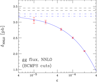
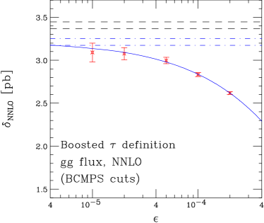
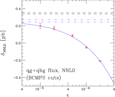
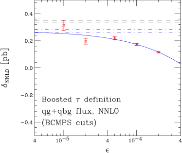
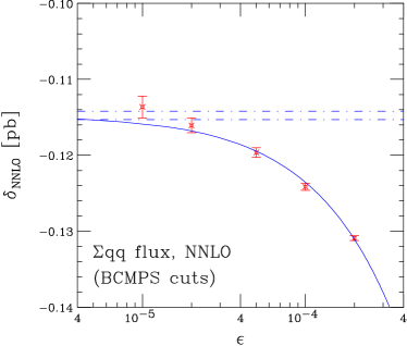
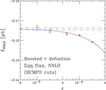
Figure 7: $\tau$-dependence of the NNLO coefficient for the $gg$, $qg+\bar{q}g$ and four-quark partonic channels using the setup of BCMPS. The plots on the left-hand side show the results with ${\mathcal{T}}_{1}$ computed in the hadronic c.o.m. while those on the right are obtained using the boosted definition. The black dashed lines indicate the BCMPS result, including the uncertainty, and the bands enclosed by the blue dot-dashed lines show the error on the asymptotic value obtained from the fitted blue curve.

Results obtained using this setup are shown in Fig. 7, once again for both definitions of ${\mathcal{T}}_{1}$. As before we see that the boosted definition is subject to much weaker power corrections, resulting in a much quicker approach to the asymptotic result. For example, at the lowest value of $\tau\textsubscript{cut}$ considered here, corresponding to $\epsilon=10^{-5}$, the deviation from the asymptotic fit value – obtained using the same fit forms as in Section III – is around $4\%$ for the $gg$ channel. We note that this value of $\tau\textsubscript{cut}$ is as small as practically possible for our code, with much lower values becoming sensitive to numerical instability in the evaluation of the double-real contributions. However, we observe that the asymptotic results obtained from this fit to the power corrections indicate somewhat smaller NNLO corrections to the $gg$ and $qg$ channels than those found by BCMPS. The asymptotic results for each channel are,

$$\delta_{NNLO}^{gg,fit}=3.213\pm 0.040\,\text{pb}\,,$$

$$\delta_{NNLO}^{qg+\bar{q}g,fit}=0.272\pm 0.013\,\text{pb}\,.$$ (16)

Both results are lower than BCMPS (c.f. Table 4), by about $6\%$ ($gg$) and $21\%$ ($qg$), and outside the error bands on the calculations ($1.2\%$ and $5\%$, respectively). However, we note that the BCMPS results reported in Table 4 and Fig. 7 contain error estimates that may not be reliable for such a detailed comparison; they may be underestimated by a factor of around three. A small difference would still remain for the $qg$ channel even after taking this into account, which we suspect may be due to our calculation being unable to go to sufficiently low values of $\tau\textsubscript{cut}$ to reliably extract the asymptotic result. Taking the original error estimates at face value, the combined effect is a $1.1$% difference in the total NNLO cross section – insufficient to conclusively establish agreement between the calculations in this region but mostly harmless for phenomenological studies.

Fig. 7 also shows the result of the computation of the correction to the 4-quark channels ($qq$, $\bar{q}\bar{q}$, and $q\bar{q}$). Our results verify the size of these corrections at NNLO, with the fitted asymptotic result,

$$\delta_{NNLO}^{\sum qq,fit}=-0.114\pm 0.001\,\text{pb}\,.$$ (17)

This demonstrates that the corrections are of a similar size as the NLO ones, but are at the level of $0.5\%$ in the total cross-section and therefore negligible for the purposes of present phenomenology.

V Boosted region

We conclude our study with an examination of the performance of the jettiness slicing method in a region for which it is especially well-suited. For illustration we consider the calculation of the cross-section in the boosted region corresponding to a recent CMS analysis searching for the decay $H\to b\bar{b}$ Sirunyan et al. (2018). This analysis reconstructs Higgs boson candidates that satisfy $p_{T}^{H}>450$ GeV, for which the leading theoretical contribution is a Higgs boson recoiling against a jet of the same transverse momentum. The cut on $p_{T}^{H}$ allows a well-defined calculation to be performed at fixed perturbative order, although at higher orders the cross-section receives contributions from partons of lower momenta. Nevertheless, at NNLO such contributions satisfy $p_{T}>p_{T}^{H}/3$, which is still a much stronger constraint than any of the scenarios studied so far. We therefore expect the jettiness slicing method to be subject to much smaller power corrections. Finally we note that the calculation presented here should not be compared directly with experimental data since, as is well-known, the effective field theory used to perform the calculation is not valid in the region $p_{T}^{H}>m_{t}$. Instead one must take into account the effect of a finite top-quark mass, for example as in Ref. Chen et al. (2016), a procedure that can now be performed using exact results at NLO Jones et al. (2018). Here we refrain from such an approach in order to focus instead on the efficacy of the jettiness method itself.

We modify our parameters only slightly for this study. We use the same setup as in the previous section, with the exception that we modify the scale choice in order to take into account the transverse momentum of the Higgs boson. We thus use,

$$\mu_{R}=\mu_{F}=\sqrt{m_{H}^{2}+\left(p_{T}^{H}\right)^{2}}$$ (18)

and drop any jet requirement, replacing this with the cut $p_{T}^{H}>450$ GeV. Here we choose to quote cross-sections that do not include any pseudo-rapidity cut on the Higgs boson, in contrast to the CMS analysis Sirunyan et al. (2018). We note instead that such a cut has almost no effect on the theoretical calculation, reducing the cross-section by $0.1\%$. For the jettiness slicing calculation we modify the definition of $\tau\textsubscript{cut}$ in order to reflect the role of the transverse momentum of the Higgs boson, rather than that of the jet, in the definition of the hardness of the process,

$$\tau\textsubscript{cut}=\epsilon\times\sqrt{m_{H}^{2}+\left(p_{T}^{H}\right)^{2}}\,.$$ (19)

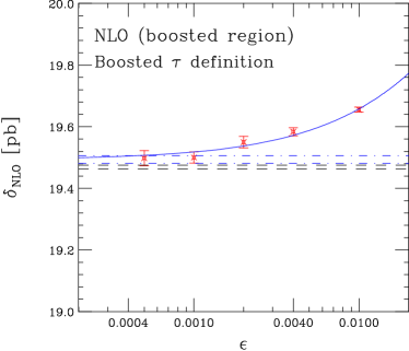
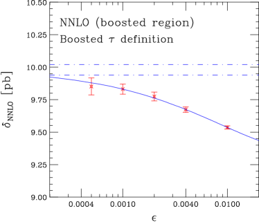
Figure 8: $\tau$-dependence of NLO (left) and NNLO (right) coefficients for Higgs boson production in the boosted regime, $p_{T}^{H}>450$ GeV. The (blue) solid lines correspond to the fit forms in Eqs. (7) and (8), with the dot-dashed lines representing the errors on the asymptotic value of the fit. For the NLO coefficient the exact result computed in MCFM using dipole subtraction is shown as the black dashed line.

The expectation of reduced power corrections in the boosted region is first confirmed by the results of a study at NLO, shown in Fig. 8 (left). In this case the jettiness slicing results agree with those of the exact calculation at NLO, to within 0.6%, even for $\epsilon=4\times 10^{-3}$. For comparison, we observe that a similar level of agreement for the jet cut in Section III ($p_{T}^{\text{jet}}>30$ GeV) is only obtained for $\epsilon=2\times 10^{-4}$ . From Fig. 8 (right) it is clear that the calculation of the NNLO coefficient is similarly improved in the boosted region, with the agreement between the fit result and the point at $\epsilon=10^{-3}$ already at the $1.5$% level. When combined with the NLO cross-section,

$$\sigma_{NLO}(p_{T}^{H}>450~{}\mbox{GeV})=40.67\,\text{pb}\,,$$ (20)

we find,

$$\sigma_{NNLO}(p_{T}^{H}>450~{}\mbox{GeV},\epsilon=10^{-3})=50.50\pm 0.04\,\text{pb}\,.$$ (21)

Therefore the difference between this result and the one that would be obtained with the asymptotic fit is around $0.3\%$, well below the level of phenomenological interest. We note in passing that the effect of the NNLO corrections on the boosted cross-section is only slightly larger than at lower transverse momenta.

VI Conclusions

In this paper we have presented a calculation of $H$+jet production at NNLO using the $N$-jettiness procedure. This calculation shares many elements with an earlier computation using the same method Boughezal et al. (2015b), but differs in the exact implementation. In particular, small errors in the above-cut $H+2$ jet NLO calculation have been corrected and the analysis has been performed at smaller values of the jettiness-slicing parameter, $\tau\textsubscript{cut}$. We have compared results with other calculations available in the literature Chen et al. (2015, 2016); Bizon et al. (2018); Boughezal et al. (2015a) and found good agreement. As anticipated from the jet cuts used for the comparisons, in particular the relatively low transverse momenta and lack of any rapidity requirement, the $N$-jettiness calculations suffers from relatively large power corrections. These can be ameliorated by using a definition of $1$-jettiness that accounts for the boost of the Higgs+jet system. For these comparisons we showed that it is possible to determine the NNLO coefficient $\delta_{NNLO}$ with an accuracy of around $5\%$ with reasonable numerical stability, but that substantially better agreement can only be obtained by fitting out the effect of power corrections. On the other hand, since $\delta_{NNLO}/\sigma_{NNLO}\approx 1/6$, an accuracy of $5\%$ in the NNLO coefficient translates into an error on the total rate, $\sigma_{NNLO}$, of less than $1\%$. We also showed that requiring a substantially harder jet reduces the effect of power corrections considerably and renders the method more competitive. Our calculation demonstrates the importance of a dedicated program to compute the effects of power corrections analytically, as has already been performed for the color-singlet case Moult et al. (2017); Boughezal et al. (2017b); Moult et al. (2018); Boughezal et al. (2018); Ebert et al. (2018), in order to improve the effectiveness of the $N$-jettiness method.

References

- Boughezal et al. (2013) R. Boughezal, F. Caola, K. Melnikov, F. Petriello, and M. Schulze, JHEP 06, 072 (2013), arXiv:1302.6216 [hep-ph] .
- Chen et al. (2015) X. Chen, T. Gehrmann, E. W. N. Glover, and M. Jaquier, Phys. Lett. B740, 147 (2015), arXiv:1408.5325 [hep-ph] .
- Boughezal et al. (2015a) R. Boughezal, F. Caola, K. Melnikov, F. Petriello, and M. Schulze, Phys. Rev. Lett. 115, 082003 (2015a), arXiv:1504.07922 [hep-ph] .
- Boughezal et al. (2015b) R. Boughezal, C. Focke, W. Giele, X. Liu, and F. Petriello, Phys. Lett. B748, 5 (2015b), arXiv:1505.03893 [hep-ph] .
- Caola et al. (2015) F. Caola, K. Melnikov, and M. Schulze, Phys. Rev. D92, 074032 (2015), arXiv:1508.02684 [hep-ph] .
- Chen et al. (2016) X. Chen, J. Cruz-Martinez, T. Gehrmann, E. W. N. Glover, and M. Jaquier, JHEP 10, 066 (2016), arXiv:1607.08817 [hep-ph] .
- Chen et al. (2019) X. Chen, T. Gehrmann, E. W. N. Glover, A. Huss, Y. Li, D. Neill, M. Schulze, I. W. Stewart, and H. X. Zhu, Phys. Lett. B788, 425 (2019), arXiv:1805.00736 [hep-ph] .
- Bizon et al. (2018) W. Bizon, X. Chen, A. Gehrmann-De Ridder, T. Gehrmann, N. Glover, A. Huss, P. F. Monni, E. Re, L. Rottoli, and P. Torrielli, JHEP 12, 132 (2018), arXiv:1805.05916 [hep-ph] .
- de Florian et al. (2016) D. de Florian et al. (LHC Higgs Cross Section Working Group), (2016), 10.23731/CYRM-2017-002, arXiv:1610.07922 [hep-ph] .
- Boughezal et al. (2015c) R. Boughezal, C. Focke, X. Liu, and F. Petriello, Phys. Rev. Lett. 115, 062002 (2015c), arXiv:1504.02131 [hep-ph] .
- Gaunt et al. (2015) J. Gaunt, M. Stahlhofen, F. J. Tackmann, and J. R. Walsh, JHEP 09, 058 (2015), arXiv:1505.04794 [hep-ph] .
- Moult et al. (2017) I. Moult, L. Rothen, I. W. Stewart, F. J. Tackmann, and H. X. Zhu, Phys. Rev. D95, 074023 (2017), arXiv:1612.00450 [hep-ph] .
- Campbell et al. (2011) J. M. Campbell, R. K. Ellis, and C. Williams, JHEP 1107, 018 (2011), arXiv:1105.0020 [hep-ph] .
- Campbell et al. (2015) J. M. Campbell, R. K. Ellis, and W. T. Giele, Eur. Phys. J. C75, 246 (2015), arXiv:1503.06182 [physics.comp-ph] .
- Boughezal et al. (2017a) R. Boughezal, J. M. Campbell, R. K. Ellis, C. Focke, W. Giele, X. Liu, F. Petriello, and C. Williams, Eur. Phys. J. C77, 7 (2017a), arXiv:1605.08011 [hep-ph] .
- Campbell et al. (2017a) J. M. Campbell, R. K. Ellis, and C. Williams, Phys. Rev. Lett. 118, 222001 (2017a), arXiv:1612.04333 [hep-ph] .
- Campbell et al. (2017b) J. M. Campbell, R. K. Ellis, and C. Williams, Phys. Rev. D96, 014037 (2017b), arXiv:1703.10109 [hep-ph] .
- Gaunt et al. (2014a) J. R. Gaunt, M. Stahlhofen, and F. J. Tackmann, JHEP 04, 113 (2014a), arXiv:1401.5478 [hep-ph] .
- Gaunt et al. (2014b) J. Gaunt, M. Stahlhofen, and F. J. Tackmann, JHEP 08, 020 (2014b), arXiv:1405.1044 [hep-ph] .
- Becher and Neubert (2006) T. Becher and M. Neubert, Phys. Lett. B637, 251 (2006), arXiv:hep-ph/0603140 [hep-ph] .
- Becher and Bell (2011) T. Becher and G. Bell, Phys. Lett. B695, 252 (2011), arXiv:1008.1936 [hep-ph] .
- Campbell et al. (2018) J. M. Campbell, R. K. Ellis, R. Mondini, and C. Williams, Eur. Phys. J. C78, 234 (2018), arXiv:1711.09984 [hep-ph] .
- Boughezal et al. (2015d) R. Boughezal, X. Liu, and F. Petriello, Phys. Rev. D91, 094035 (2015d), arXiv:1504.02540 [hep-ph] .
- Bell et al. (2018) G. Bell, B. Dehnadi, T. Mohrmann, and R. Rahn, Proceedings, 14th DESY Workshop on Elementary Particle Physics: Loops and Legs in Quantum Field Theory 2018 (LL2018): St. Goar, Germany, April 29-May 04, 2018, PoS LL2018, 044 (2018), arXiv:1808.07427 [hep-ph] .
- Becher et al. (2014) T. Becher, G. Bell, C. Lorentzen, and S. Marti, JHEP 02, 004 (2014), arXiv:1309.3245 [hep-ph] .
- Gehrmann et al. (2012) T. Gehrmann, M. Jaquier, E. W. N. Glover, and A. Koukoutsakis, JHEP 02, 056 (2012), arXiv:1112.3554 [hep-ph] .
- Jouttenus et al. (2011) T. T. Jouttenus, I. W. Stewart, F. J. Tackmann, and W. J. Waalewijn, Phys. Rev. D83, 114030 (2011), arXiv:1102.4344 [hep-ph] .
- Jouttenus et al. (2013) T. T. Jouttenus, I. W. Stewart, F. J. Tackmann, and W. J. Waalewijn, Phys. Rev. D88, 054031 (2013), arXiv:1302.0846 [hep-ph] .
- Boughezal et al. (2016) R. Boughezal, J. M. Campbell, R. K. Ellis, C. Focke, W. T. Giele, X. Liu, and F. Petriello, Phys. Rev. Lett. 116, 152001 (2016), arXiv:1512.01291 [hep-ph] .
- Campbell et al. (2016a) J. M. Campbell, R. K. Ellis, and C. Williams, JHEP 06, 179 (2016a), arXiv:1601.00658 [hep-ph] .
- Campbell et al. (2016b) J. M. Campbell, R. K. Ellis, Y. Li, and C. Williams, JHEP 07, 148 (2016b), arXiv:1603.02663 [hep-ph] .
- Alwall et al. (2014) J. Alwall, R. Frederix, S. Frixione, V. Hirschi, F. Maltoni, O. Mattelaer, H. S. Shao, T. Stelzer, P. Torrielli, and M. Zaro, JHEP 07, 079 (2014), arXiv:1405.0301 [hep-ph] .
- Nagy and Trocsanyi (1999) Z. Nagy and Z. Trocsanyi, Phys. Rev. D59, 014020 (1999), [Erratum: Phys. Rev.D62,099902(2000)], arXiv:hep-ph/9806317 [hep-ph] .
- Dawson (1991) S. Dawson, Nucl. Phys. B359, 283 (1991).
- Chetyrkin et al. (1997) K. G. Chetyrkin, B. A. Kniehl, and M. Steinhauser, Phys. Rev. Lett. 79, 353 (1997), arXiv:hep-ph/9705240 [hep-ph] .
- Ebert et al. (2018) M. A. Ebert, I. Moult, I. W. Stewart, F. J. Tackmann, G. Vita, and H. X. Zhu, JHEP 12, 084 (2018), arXiv:1807.10764 [hep-ph] .
- Sirunyan et al. (2018) A. M. Sirunyan et al. (CMS), Phys. Rev. Lett. 120, 071802 (2018), arXiv:1709.05543 [hep-ex] .
- Jones et al. (2018) S. P. Jones, M. Kerner, and G. Luisoni, Phys. Rev. Lett. 120, 162001 (2018), arXiv:1802.00349 [hep-ph] .
- Boughezal et al. (2017b) R. Boughezal, X. Liu, and F. Petriello, JHEP 03, 160 (2017b), arXiv:1612.02911 [hep-ph] .
- Moult et al. (2018) I. Moult, L. Rothen, I. W. Stewart, F. J. Tackmann, and H. X. Zhu, Phys. Rev. D97, 014013 (2018), arXiv:1710.03227 [hep-ph] .
- Boughezal et al. (2018) R. Boughezal, A. Isgrò, and F. Petriello, Phys. Rev. D97, 076006 (2018), arXiv:1802.00456 [hep-ph] .