$\bm{B\to D^{\ast}\ell\nu}$ at non-zero recoil

Abstract

The current status of the lattice-QCD calculations of the form factors of the $B\to D^{\ast}\ell\nu$ semileptonic decay is reviewed. Particular emphasis is given to the most mature calculation at non-zero recoil coming from the Fermilab Lattice and MILC collaborations. Blinded, preliminary results for the form factors are shown, including a preliminary, but detailed error budget. The lattice results seem to favor a large slope at small recoil, in contrast to the latest untagged results coming from the Belle collaboration. A comprehensive comparison between the latest BGL $z$ expansions of Belle, Babar, the lattice and a joint BGL fit including lattice and Belle data is presented, and a roadmap to improve the current calculation is discussed. The current implications for $V_{cb}$ and $R(D^{\ast})$ are discussed.

I Introduction

During the last few years the CKM Cabibbo:1963yz ; Kobayashi:1973fv matrix element $V_{cb}$ has been at the center of a discussion regarding the unitarity triangle and the search for new physics. According to the latest HFLAV report Amhis:2016xyh and subsequent updates, there is a $\approx 2\sigma$ tension between the inclusive and the exclusive determinations. In addition there is a combined $\approx 3\sigma$ tension between the Standard Model (SM) predictions and experimental measurements in the $R(D)$-$R(D^{\ast})$ plane. Recently a promising proposal found a way to reconcile the long-standing inclusive vs exclusive discrepancy BIGI2017441 ; GRINSTEIN2017359 : the CLN parametrization Caprini:1997mu is becoming too restrictive, given the current precision of experiments, and some of its assumptions should be revisited. In contrast, the BGL parametrization Boyd:1997kz offers a model-independent alternative, free from precision errors. Once BGL is used to extrapolate the experimental data to zero recoil, the $V_{cb}$ discrepancy disappears. The fact that until very recently most experimental results were only published in terms of the CLN parameters fueled the controversy.

Belle was the first collaboration to publish unfolded data with their tagged analysis BelleTagged . More recently, a second dataset coming from an untagged analysis was published BelleUntagged , along with their results for a BGL fit that disagrees with the inclusive result. In light of these recent developments, the Babar collaboration also decided to rerun their analysis using the BGL parametrization, finding that the disagreement between inclusive and exclusive still stands. Thus, even though there is some evidence that the CLN parametrization Caprini:1997mu is not optimal, our woes and worries about $V_{cb}$ are far from being solved.

In this context, a lattice-QCD calculation of the form factors involved in the decay at non-zero recoil is urgent and necessary. Lattice-QCD data can help settle the parametrization issue, as well as provide reliable results in the low recoil region, which is most prone to experimental errors. We expect the current value of $V_{cb}$ to change as a result of lattice efforts. On top of that, a lattice $R(D^{\ast})$ calculation would be very welcome. Although a variety of other calculations exist Fajfer:2012vx ; Bernlochner:2017jka ; Bigi:2017jbd ; Jaiswal:2017rve , none of them comes from lattice gauge theory, the only first-principles, non-perturbative tool available to tackle QCD.

In this work we present the current status of the ongoing lattice-QCD calculations of the $B\to D^{\ast}\ell\nu$ semileptonmic decay form factors. We emphasize the preliminary results coming from the most mature calculation, and we compare the current available experimental results with the preliminary predictions coming from the lattice.

II Notation and definitions

The Standard Model prediction for the differential rate for exclusive $B\to D^{*}\ell\nu$ decay can be written in terms of the recoil parameter $w=v_{D^{\ast}}\cdot v_{B}$,

$$\frac{d\Gamma}{dw}\left(B\to D^{\ast}\ell\nu\right)=\frac{G_{F}m_{B}^{5}}{48\pi^{2}}\left(1-r^{2}\right)\sqrt{w^{2}-1}\,\chi(w)\left|\eta_{\rm{EW}}\right|^{2}\left|V_{cb}\right|^{2}\left|\mathcal{F}(w)\right|^{2},$$ (1)

where $v_{X}=p_{X}/m_{X}$ are the four velocities of the $B$ and $D^{\ast}$ mesons, $\eta_{\rm{EW}}$ is a correction factor that accounts for electroweak effects, $r=m_{D^{\ast}}/m_{B}$, $\mathcal{F}(w)$ is a function that represents the probability amplitude, to be calculated in theory, and $\chi(w)$ gathers all the remaining kinematic factors. The function $\mathcal{F}$ can be expressed in terms of the helicity amplitudes $H_{\pm,0}$ as,

$$\chi(w)\left|\mathcal{F}(w)\right|^{2}=\frac{1-2wr+r^{2}}{12m_{B}m_{D^{\ast}}(1-r)^{2}}\left(H_{0}^{2}(w)+H_{+}^{2}(w)+H_{-}^{2}(w)\right).$$ (2)

The helicity amplitudes, in turn, depend on the $h_{X}(w)$ form factors, motivated by heavy quark effective theory (HQET),

$$H_{0}(w)= \frac{\sqrt{m_{B}m_{D^{\ast}}}}{1-2wr+r^{2}}(w+1)\left[(w-r)h_{A_{1}}(w)-(w-1)(rh_{A_{2}}(w)+h_{A_{3}}(2))\right],$$ (3)

$$H_{\pm}(w)= \sqrt{m_{B}m_{D^{\ast}}}(w+1)\left(h_{A_{1}}(w)\pm\sqrt{\frac{w-1}{w+1}}h_{V}(w)\right).$$ (4)

The form factors are defined following the standard decomposition of the matrix elements of the $V-A$ weak current that mediates the transition,

$$\frac{\left\langle D^{\ast}(p_{D^{\ast}},\epsilon^{\nu})\right|\mathcal{V}^{\mu}\left|B(0)\right\rangle}{2\sqrt{m_{B}m_{D^{\ast}}}}= \frac{1}{2}\epsilon^{\ast}_{\nu}\varepsilon^{\mu\nu}_{\sigma\rho}v_{D^{\ast}}^{\sigma}v_{B}^{\rho}\,h_{V}(w),$$ (5)

$$\frac{\left\langle D^{\ast}(p_{D^{\ast}},\epsilon^{\nu})\right|\mathcal{A}^{\mu}\left|B(0)\right\rangle}{2\sqrt{m_{B}m_{D^{\ast}}}}= \frac{i}{2}\epsilon^{\ast}_{\nu}\left[g^{\mu\nu}(1+w)h_{A_{1}}(w)-v_{B}^{\nu}\left(v_{B}^{\mu}h_{A_{2}}(w)+v_{D^{\ast}}^{\mu}h_{A_{3}}(w)\right)\right].$$ (6)

Up to very recently, only zero-recoil ($w=1$) results were available for the decay amplitude $\mathcal{F}(w)$ in (1). HQET calculations can access only the zero recoil region because, as soon as $w$ deviates from one, non-perturbative effects become important, and we don’t know how to calculate them without resorting to lattice-QCD. On the other hand, lattice-QCD calculations at non-zero recoil are extremely complicated, and had not been tackled until the last years.

Experiments measure the differential decay rate (1), but since the kinematic factor is proportional to $\sqrt{w^{2}-1}$, it is not feasible to measure it directly at zero recoil. Hence, we must rely on extrapolations in order to extract $V_{cb}$ from a joint effort coming from experiment and theory. The most popular parametrizations for this decay are BGL Boyd:1997kz and CLN Caprini:1997mu . The parametrizations are explained in section IV.

III Status of the lattice calculation

Lattice-QCD allows for a direct calculation of the form factors defined in eqs. (5,6) at zero and non-zero recoil. Currently only zero-recoil calculations are available, where only $h_{A_{1}}$ contributes to the decay amplitude. The Fermilab Lattice and MILC collaborations Lattice:2015rga use the asqtad ($a-$squared, tadpole improved) action for the light sea and valence quarks, and the Fermilab effective action for the heavy quarks. It employs 15 ensembles with lattice spacings ranging from $0.045$ fm up to $0.15$ fm, and pion masses from $500$ MeV down to $180$ MeV. Their result is $\mathcal{F}(1)=0.906\pm 0.004_{\textrm{Stat}}\pm 0.012_{\textrm{Sys}}$. The HPQCD collaboration Harrison:2017fmw has published results using 8 ensembles with the HISQ (Highly Improved Staggered Quark) action for the sea and valence quarks, and using NRQCD for the bottom quark. Here the sea includes charm. They use lattice spacings ranging from $0.15$ fm to $0.09$ fm and pion masses from $320$ MeV up to the physical value. Their final result is $\mathcal{F}(1)=0.895\pm 0.010_{\textrm{Stat}}\pm 0.024_{\textrm{Sys}}$. Even though HPQCD uses a superior light quark action and physical pion mass ensembles, they obtain larger errors due to the mismatch between the bottom and the charm quark regularization; this mismatch introduces larger renormalization errors than in the Fermilab/MILC result. A second calculation by HPQCD focuses on $B_{s}\to D_{s}^{\ast}\ell\nu$ HPQCD2 . It also uses the HISQ regularization for the bottom quark, but at an unphysical mass, requiring an extrapolation to reach the right value. Nevertheless, the use of the same actions for the $B$ and the $D^{\ast}$ results in a much more accurate value than in their previous approach that used NRQCD. From their result for $\mathcal{F}_{s}(1)$ they extract $\mathcal{F}(1)$ by using the $\mathcal{F}(1)/\mathcal{F}_{s}(1)$ ratio computed in Harrison:2017fmw . Their final result is $\mathcal{F}(1)=0.914\pm 0.024$, in agreement with their previous result and with the Fermilab/MILC calculation. The fact that these independent calculations using different regularizations for the light and the heavy quarks –with totally different systematic errors– agree, is an indication of the reliability of the lattice calculations. There is an ongoing fourth calculation coming from the SWME and LANL collaborations Bhattacharya:2018gan based on the Oktay-Kronfeld action OKref for the bottom and charm quarks. Fig.1 shows their current preliminary results, along with the previous results of HPQCD and Fermilab/MILC.

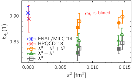
Figure 1: Status of the zero recoil LANL/SWME calculation. Here $\lambda\sim\Lambda_{\rm{QCD}}/2m_{c}$ and $\lambda^{n}$ refers to the highest HQET term included in the matching procedure. Plot taken from the slides of the KEK-FF2019 meeting KKOK , courtesy of the authors.

For non-zero recoil, the calculation becomes much more involved. As shown in Eqs. (5) and (6), there are four different form factors to compute. One should expect that the correlations among them are very strong, because they share underlying gauge configurations, propagators and three-point functions in their calculations. Currently there are no calculations available, but two efforts are underway: the JLQCD collaboration is working on a calculation based on domain-wall fermions Kaneko:2018mcr . They include the charm quark in the sea, and the bottom quark has an unphysical mass. Then they extrapolate to the correct bottom mass. They have presented status updates in previous conferences (see Fig. 2). The other calculation comes from Fermilab/MILC Aviles-Casco:2017nge ; Aviles-Casco:2019vin , and it is in its final stages of development. We use the same ensembles and regularization as in our previous zero recoil calculation, and we publish regular updates on our analysis. Preliminary, blinded results for our form factors are shown in Figs. 3-6. The bands here represent the final result in the continuum, after the chiral-continuum limit has been taken. The four form factors were fitted at the same time with $p=0.36$.

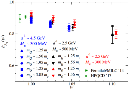
Figure 2: Preliminary lattice results of the non-zero recoil JLQCD calculation for $h_{A_{1}}$. The collaboration is calculating the four relevant form factors. Taken from the slides of the KEK-FF2019 meeting KKJLQCD , courtesy of the authors.

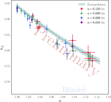
Figure 3: Blinded, preliminary results of the Fermilab/MILC calculation for $h_{A_{1}}$. The points represent the lattice data and the band is the final result extrapolated, to the continuum.

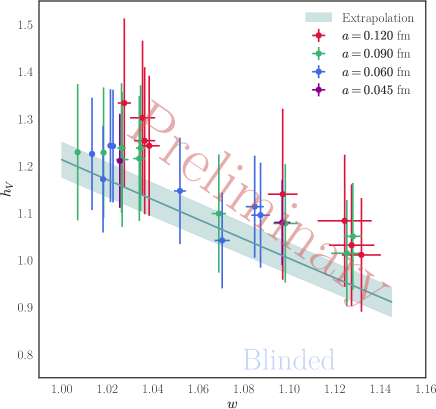
Figure 4: Blinded, preliminary results of the Fermilab/MILC calculation for $h_{V}$. The points represent the lattice data and the band is the final result extrapolated, to the continuum.

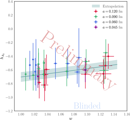
Figure 5: Blinded, preliminary results of the Fermilab/MILC calculation for $h_{A_{2}}$. The points represent the lattice data and the band is the final result extrapolated, to the continuum.

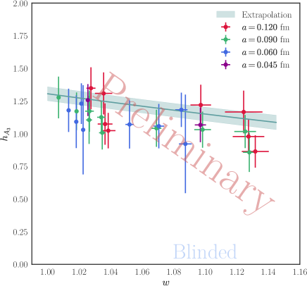
Figure 6: Blinded, preliminary results of the Fermilab/MILC calculation for $h_{A_{3}}$. The points represent the lattice data and the band is the final result extrapolated, to the continuum.

III.1 Preliminary error budget

Table 1 gathers the preliminary error budget of the Fermilab/MILC calculation for the different form factors. The errors depend on the recoil parameter, and the table shows the values at $w\sim 1.10$. We have a well defined roadmap to reduce these errors in three steps, and this calculation is the first of these steps.

Table 1: Preliminary error budget at $w\sim 1.10$.

Source	$h_{V}\,(\%)$	$h_{A_{1}}\,(\%)$	$h_{A_{2}}\,(\%)$	$h_{A_{3}}\,(\%)$
Statistics	$1.1$	$0.4$	$4.9$	$1.9$
Isospin effects	$0.0$	$0.0$	$0.6$	$0.3$
$\chi$PT/cont. extrap.	$1.9$	$0.7$	$6.3$	$2.9$
Matching	$1.5$	$0.4$	$0.1$	$1.5$
Heavy quark discr.	$1.4^{*}$	$0.4^{*}$	$5.8^{*}$	$1.3^{*}$

^∗Estimate, currently subject of intensive study.

The main source of systematic errors currently come from the chiral-continuum extrapolation, which uses EFTs (Effective Field Theories) to take the lattice data to the continuum limit, where the lattice spacing becomes zero, and takes the quark masses to their physical values. The use of EFTs allow us to control the systematic errors and to have a good ansatz for the extrapolation. We plan to reduce these errors dramatically in the second step of our roadmap, by using HISQ quarks for the light sector at smaller lattice spacings and lower pion masses, reaching physical pions in some ensembles. We plan to keep using the Fermilab action for the charm and the bottom quarks in this first iteration.

The next important source of error comes from the discretization of the heavy quarks. The large mass of the heavy quarks makes them problematic to simulate on the lattice: since their Compton wavelength is extremely small, they require an accordingly small lattice spacing to be simulated properly, otherwise one incurs large discretization errors. Effective heavy quark actions are used to mitigate these effects, and in our case we employ the Fermilab action, which removes tree-level discretization effects. But still, the remaining errors constitute a large component of our current error budget. In the third and final step of our roadmap, we plan to replace the heavy quark action with HISQ fermions as well, and simulate the bottom quark as if it were a light quark. This improvement is expected to removed most of the discretization errors in our calculation.

The third large source of errors is the renormalization and the matching. Currents on the lattice do not have the same symmetries as currents in the continuum; therefore, they require proper renormalization. In our calculation we compute ratios of three-point functions, where most of the renormalization factors cancel, but we must compute the remainder using perturbation theory. Currently our calculations allow us to compute these factors at zero recoil, so we add a conservative error in order to take into account that our form factors are evaluated at non-zero recoil. This error turns out to be sizeable. Our final iteration of the analysis with HISQ heavy quarks will use fully non-perturbative renormalization, which is expected to reduce these errors to negligible values.

The other source of systematic errors, isospin breaking, comes from the fact that in our lattice simulations we simulate with degenerate up and down quarks. This error is small compared with the other contributions.

Once the form factors are calculated on the lattice, one can use any existing parametrization to extrapolate to the whole kinematic range with improved precision. Since the lattice is accurate only in the small recoil region ($w\lesssim 1.1$), the parametrizations provide extremely useful information to constrain the form factors.

IV The $\bm{z}$ expansion and $\bm{V_{cb}}$

The Boyd-Grinstein-Lebed (BGL) parametrization Boyd:1997kz is built upon very general arguments. It is based on the fact that one can constrain the amplitude of the production of a pair $H_{b}\bar{H}_{c}$ from a virtual $W$ boson with $q^{2}>m_{B}^{2}+m_{D^{\ast}}^{2}$, and then propagate the constraints back to the semileptonic region, where $m_{\ell}^{2}<q^{2}<m_{B}^{2}-m_{D^{\ast}}^{2}$, by using analyticity. The process results in bounds for the form factors, which are expressed in a general form,

$$F(z)=\frac{1}{B_{F}(z)\phi_{F}(z)}\sum_{j=0}^{\infty}a^{F}_{j}z^{j},$$ (7)

where $F(z)$ is a particular form factor, $B_{F}(z)$ is the so-called Blaschke factor, which gathers the dependence of the poles relevant to our form factor $F$, $\phi_{F}(z)$ is called the outer function, and must be computed in the theory, and $z$ is a small variable coming from a comformal transformation of the recoil parameter. In the most common case, $z$ ranges from $0$ at zero recoil to its maximum value,

$$z=\frac{\sqrt{w+1}-\sqrt{2}}{\sqrt{w+1}+\sqrt{2}},$$ (8)

but Babar prefers to set $z=0$ at the point $t_{0}=(m_{B}+m_{D^{\ast}})(\sqrt{m_{B}}-\sqrt{m_{D^{\ast}}})^{2}$, a particular choice that gives a symmetric range around zero.

The unitarity constraints in the BGL parametrization are applied to the coefficients $a^{F}_{j}$ of the expansion. Given a set of form factors $\mathcal{S}$ sharing parity and spin quantum numbers, the constraint reads

$$\sum_{F\in\mathcal{S}}\sum_{j=0}^{\infty}(a^{F}_{j})^{2}\leq 1$$ (9)

These are known as the weak unitarity constraints. One can further constrain the coefficients of the expansion by considering several decays related by crossing symmetry. The new constraints are known as the strong unitarity constraints.

The Caprini-Lellouch-Neubert (CLN) parametrization Caprini:1997mu is based on the same principles as the BGL parametrization, but it builds in the strong unitarity constraints and uses some inputs based on information in 1997 to remove parameters from the more general expansion. In the end the authors present a simplified polynomial expansion,

$$h_{A_{1}}(z)= h_{A_{1}}(1)\left(1-8\rho^{2}z+\right.$$

$$\left.(53\rho^{2}-15)z^{2}-(231\rho^{2}-91)z^{3}\right),$$ (10)

$$R_{1}(w)= R_{1}(1)-0.12(w-1)+0.05(w-1)^{2},$$ (11)

$$R_{2}(w)= R_{2}(1)+0.11(w-1)-0.06(w-1)^{2},$$ (12)

where $z$ is given by Eq. (8).

V Comparison between Lattice-QCD and Experiment

With the lattice data available, one can try a pure lattice prediction of the decay amplitude $|\mathcal{F}(w)|^{2}$, fitting each form factor to its corresponding $z$ expansion, and compare it with the pure experimental fits. Experimental data can be fitted only to $\eta_{\rm{EW}}^{2}|V_{cb}|^{2}|\mathcal{F}(w)|^{2}$, but the difference is a proportionality factor, and one can readily compare the shapes of the decay amplitudes by taking out an overall normalization. This is done in Fig. 7. In Fig. 8 we show the different predictions for $\eta_{\rm{EW}}^{2}|V_{cb}|^{2}|\mathcal{F}(w)|^{2}$. We include Babar results, as in Babar , our own fit to the Belle untagged dataset and a joint fit using Belle untagged data and the lattice. We also include the data points for both Belle datasets, as well as the lattice data points multiplied by the $\eta_{\rm{EW}}^{2}|V_{cb}|^{2}$ that results from the joint lattice-Belle (untagged) fit. Since the lattice data is blinded, the final value of $\eta_{\rm{EW}}^{2}|V_{cb}|^{2}$ coming from the joint fit is blinded, but other details, such as the slope at low recoil, are not affected and a useful comparison can be done.

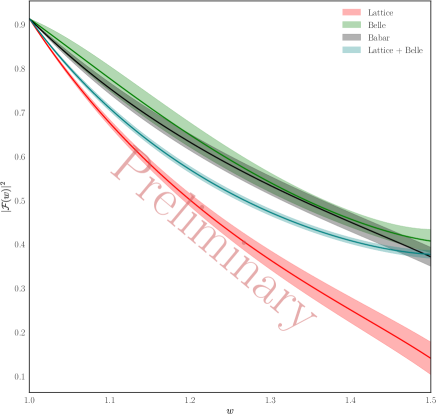
Figure 7: Predictions for $|\mathcal{F}|^{2}$ coming from the lattice, Belle, Babar and the joint fit lattice + Belle (untagged). All the curves are normalized to a common intercept at $w=1$.

The untagged Belle dataset has dramatically reduced the error of the data points. In the low recoil region, we also see a change of curvature that is not observed in the tagged dataset, since the smaller tagged sample has larger statistical errors. This seems to be at odds with the lattice preliminary prediction, which favors a large slope at small recoil. As a result, although the separate fits have reasonable $p$ values, the joint fit lattice-Belle (untagged) has a very low $p$ value. In contrast, a joint fit using the Belle tagged dataset and lattice data gives a very similar result but a reasonable $p$ value of $\gtrsim 0.5$.

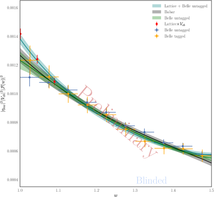
Figure 8: Results for $\eta_{\rm{EW}}^{2}|V_{cb}|^{2}|\mathcal{F}(w)|^{2}$ coming from Belle, Babar and the joint fit lattice + Belle (untagged). The $p$ values for the different fits are $p_{\textrm{Belle}}=0.09$ and $p_{\textrm{Joint}}\sim 10^{-6}$. The BaBar collaboration didn’t disclose the $p$ value in their article Babar .

One could also use the CLN parametrization for a joint fit with lattice and Belle data. In this case, no matter whether we use the tagged or the untagged dataset, the outcome of the fit is poor. The large slope at low recoil of the decay amplitude computed with lattice QCD and the shallower behavior at large recoil measured by experiment do not seem to be compatible with the CLN parametrization, which is too constraining to accommodate the tension in the slope.

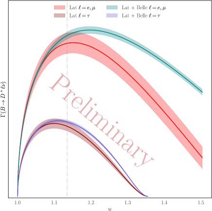
Figure 9: Decay rate as a function of $w$ for the lattice QCD calculation (reddish) and for the joint lattice QCD + untagged Belle fit (bluish). The higher set of curves is for massless leptons, whereas the lower set of curves is for the $\tau$. The vertical grey line approximately marks the maximum recoil value for which we have lattice data.

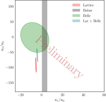
Figure 10: One sigma contour plots of the ratio of the coefficient of the $z-$expansion of the $g$ form factor in the BGL parametrization for Belle, Babar, the lattice and the joint fit lattice + Belle (untagged). The notation here is $a_{j}=a_{j}^{g}$.

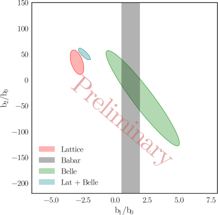
Figure 11: One sigma contour plots of the ratio of the coefficient of the $z-$expansion of the $f$ form factor in the BGL parametrization for Belle, Babar, the lattice and the joint fit lattice + Belle (untagged). The notation here is $b_{j}=a_{j}^{f}$.

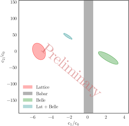
Figure 12: One sigma contour plots of the ratio of the coefficient of the $z-$expansion of the $\mathcal{F}_{1}$ form factor in the BGL parametrization for Belle, Babar, the lattice and the joint fit lattice + Belle (untagged). The notation here is $c_{j}=a_{j}^{\mathcal{F}_{1}}$.

Integrating the different predictions, we can obtain an estimate for $R(D^{\ast})$. In Fig. 9 we show the decay rate for light leptons and the $\tau$ as predicted from the lattice and from the joint fit lattice + Belle. The lattice only data is multiplied by a reasonable value of $\eta_{\rm{EW}}^{2}|V_{cb}|^{2}$, so it is properly normalized, although this normalization cancels in the calculation of the ratio. In the plot we observe a strikingly different behavior in the large recoil region. In that region, the dominant form factor of the BGL parametrization is $\mathcal{F}_{1}$, the rest are suppressed by a factor of $q^{2}$. In Figs. 10–12  we compare the ratios of the $z$ expansion coefficients of the different fits at one sigma. The fact that we are using ratios allows us to compare the lattice results with experiment, even if the lattice coefficients are blinded. Even though there are some differences in the coefficients for the $f$ and $g$ BGL form factors, the ratios would agree within a $2\sigma$ ellipsoid. The ratios for $\mathcal{F}_{1}$, in contrast, show large differences between the pure experimental results and the results involving lattice data, which explains why the curves in Fig. 9 are so different at large recoil. This behavior is currently being studied carefully.

VI Conclusions

The flavor-physics community has been facing a long-standing puzzle with the discrepancy between the inclusive and the exclusive determinations of $V_{cb}$. Two years ago, an interesting and elegant proposal was introduced GRINSTEIN2017359 ; BIGI2017441 , and that seemed to solve the problem. Lattice-QCD calculations were expected to shed light on the issue, but the preliminary lattice results and the latest experimental fits suggest that the resolution of this puzzle is more complicated than thought.

This situation calls for careful scrutiny of lattice calculations, as well as of the experimental results, in order to extract any conclusions. Hence the situation remains unclear, although with the forthcoming improvements in both experiment (Belle II) and theory we should have much more information in the coming years to make a better assessment of the puzzle. On the lattice side, very soon we will have results for two different calculations of the form factors at non-zero recoil. These calculations have very different systematic errors, and an eventual agreement would give reliability to the final result. On the other hand, the Fermilab/MILC collaboration has a very well established roadmap to improve the precision of its own calculation in three steps. Even if the current status of $V_{cb}$ is a bit uncertain, we have reason to be optimistic about the future.

- (1) N. Cabibbo, Phys. Rev. Lett. 10, 531 (1963).
- (2) M. Kobayashi and T. Maskawa, Prog. Theor. Phys. 49, 652 (1973).
- (3) Y. Amhis et al [HFLAV], arXiv:1612.07233 [hep-ex].
- (4) B. Grinstein and A. Kobach, Phys. Lett. B771, 359 (2017), arXiv:1703.08170 [hep-ph].
- (5) D. Bigi, P. Gambino and S. Schacht, Phys. Lett. B769, 441 (2017), arXiv:1703.06124 [hep-ph].
- (6) I. Caprini, L. Lellouch and M. Neubert, Nucl. Phys. B530, 153 (1998), arXiv:hep-ph/9712417.,
- (7) G. Boyd, B. Grinstein and R. Lebed, Phys. Rev. D56, 6895 (1997), arXiv:hep-ph/9705252.
- (8) A. Abdesselam et al. [Belle Collaboration], arXiv:1702.01521 [hep-ex].
- (9) A. Abdesselam et al. [Belle Collaboration], arXiv:1809.03290 [hep-ex].
- (10) J. P. Lees et al. [BaBar Collaboration], arXiv:1903.10002 [hep-ex].
- (11) S. Fajfer, J. Kamenik and I. Nisandzic, Phys. Rev. D85, 094025 (2012), arXiv:1203.2654 [hep-ph].
- (12) F. Bernlochner, Z. Ligeti, M. Papucci amd D. Robinson, Phys. Rev. D95, 115008 (2017), arXiv:1703.05330 [hep-ph].
- (13) D. Bigi, P. Gambino and S. Schacht, JHEP 1711, 061 (2017), arXiv:1707.09509 [hep-ph].
- (14) S. Jaiswal, S. Nandi and S. Patra, JHEP 1712, 060 (2017), arXiv:1707.09977 [hep-ph].
- (15) J. A. Bailey et al. [Fermilab Lattice and MILC Collaborations], Phys. Rev. D92, 034506 (2015), arXiv:1503.07237 [hep-lat].
- (16) J. Harrison et al. [HPQCD Collaboration], Phys. Rev. D97, 054502 (2018), arXiv:1711.11013 [hep-lat].
- (17) E. McLean, et al. [HPQCD Collaboration], arXiv:1904.02046 [hep-lat].
- (18) T. Bhattacharya et al., Proceedings of the Lattice 2018 conference, arXiv:1812.07675 [hep-lat].
- (19) M. Oktay and A. Kronfeld, Phys. Rev. D78, 014504 (2008), arXiv:0803.0523 [hep-lat].
- (20) Y. C. Jang on behalf of the LANL/SWME Collaboration, talk presented at the 6 KEK Flavor Factory Workshop, https://conference-indico.kek.jp/indico/event/50.
- (21) T. Kaneko et al. [JLQCD Collaboration], Proceedings of the Lattice 2018 conference, arXiv:1811.00794 [hep-lat].
- (22) A. Vaquero Avilés-Casco, C. DeTar, D. Du, A. El-Khadra, A. S. Kronfeld, J. Laiho and R. S. Van de Water [Fermilab Lattice and MILC Collaborations], EPJ Web Conf. 175, 13003 (2018), arXiv:1710.09817 [hep-lat].
- (23) A. V. Avilés-Casco, C. DeTar, A. X. El-Khadra, A. S. Kronfeld, J. Laiho and R. S. Van de Water [Fermilab Lattice and MILC Collaborations], PoS LATTICE 2018, 282 (2018), arXiv:1901.00216 [hep-lat].
- (24) T. Kaneko on behalf of the JLQCD Collaboration, talk presented at the 6 KEK Flavor Factory Workshop, https://conference-indico.kek.jp/indico/event/50.