DAve-QN: A Distributed Averaged Quasi-Newton Method with Local Superlinear Convergence Rate

Abstract

In this paper, we consider distributed algorithms for solving the empirical risk minimization problem under the master/worker communication model. We develop a distributed asynchronous quasi-Newton algorithm that can achieve superlinear convergence. To our knowledge, this is the first distributed asynchronous algorithm with superlinear convergence guarantees. Our algorithm is communication-efficient in the sense that at every iteration the master node and workers communicate vectors of size $O(p)$, where $p$ is the dimension of the decision variable. The proposed method is based on a distributed asynchronous averaging scheme of decision vectors and gradients in a way to effectively capture the local Hessian information of the objective function. Our convergence theory supports asynchronous computations subject to both bounded delays and unbounded delays with a bounded time-average. Unlike in the majority of asynchronous optimization literature, we do not require choosing smaller stepsize when delays are huge. We provide numerical experiments that match our theoretical results and showcase significant improvement comparing to state-of-the-art distributed algorithms.

1 Introduction

Many optimization problems in machine learning including empirical risk minimization are based on processing large amounts of data as an input. Due to the advances in sensing technologies and storage capabilities the size of the data we can collect and store increases at an exponential manner. As a consequence, a single machine (processor) is typically not capable of processing and storing all the samples of a dataset. To solve such “big data” problems, we typically rely on distributed architectures where the data is distributed over several machines that reside on a communication network [1, 2]. In such modern architectures, the cost of communication is typically orders of magnitude larger than the cost of floating point operation costs and the gap is increasing [3]. This requires development of distributed optimization algorithms that can find the right trade-off between the cost of local computations and that of communications.

In this paper, we focus on distributed algorithms for empirical risk minimization problems. The setting is as follows: Given $n$ machines, each machine has access to $m_{i}$ samples $\{\xi_{i,j}\}_{j=1}^{m_{i}}$ for $i=1,2,\dots,n$. The samples $\xi_{i,j}$ are random variables supported on a set $\mathcal{P}\subset{\mathbb{R}}^{d}$. Each machine has a loss function that is averaged over the local dataset:

$$f_{i}({\mathbf{x}})=\frac{1}{m_{i}}\sum_{i=1}^{m_{i}}\phi({\mathbf{x}},\xi_{i,j})+\frac{\lambda}{2}\|{\mathbf{x}}\|_{2}^{2}$$

where the function $\phi:{\mathbb{R}}^{p}\times{\mathbb{R}}^{d}\to{\mathbb{R}}$ is convex in ${\mathbf{x}}$ for each $\xi\in{\mathbb{R}}^{d}$ fixed and $\lambda\geq 0$ is a regularization parameter. The goal is to develop communication-efficient distributed algorithms to minimize the overall empirical loss defined by

$${\mathbf{x}}^{*}\coloneqq\operatornamewithlimits{argmin}_{{\mathbf{x}}\in{\mathbb{R}}^{p}}f({\mathbf{x}})\coloneqq\operatornamewithlimits{argmin}_{{\mathbf{x}}\in{\mathbb{R}}^{p}}\frac{1}{n}\sum_{i=1}^{n}f_{i}({\mathbf{x}}).$$ (1)

The communication model we consider is the centralized communication model, also known as the master/worker model [4]. In this model, the master machine possesses a copy of the global decision variable ${\mathbf{x}}$ which is shared with the worker machines. Each worker performs local computations based on its local data which is then communicated to the master node to update the decision variable. The way communications are handled can be synchronous or asynchronous, resulting in different type of optimization algorithms and convergence guarantees. The merit of synchronization is that it prevents workers from using obsolete information and, thereby, from submitting a low quality update of parameters to the master. The price to pay, however, is that all the nodes have to wait for the slowest worker, which leads to unnecessary overheads. Asynchronous algorithms do not suffer from this issue, maximizing the efficiency of the workers while minimizing the system overheads. Asynchronous algorithms are particularly preferable over networks with heterogeneous machines with different memory capacities, work overloads, and processing capabilities.

There has been a number of distributed algorithms suggested in the literature to solve the empirical risk minimization problem (1) based on primal first-order methods [5, 6, 7], their accelerated or variance-reduced versions [8, 9, 10, 11, 12], lock-free parallel methods [2, 13], coordinate descent-based approaches [4, 14, 15, 16], dual methods [17, 15], primal-dual methods [4, 18, 19, 16, 20], distributed ADMM-like methods [21] as well as quasi-Newton approaches [22, 23], inexact second-order methods [24, 25, 26, 27, 28, 29] and general-purpose frameworks for distributed computing environments [18, 19] both in the asynchronous and synchronous setting. The efficiency of these algorithms is typically measured by the communication complexity which is defined as the equivalent number of vectors in $\mathbb{R}^{p}$ sent or received across all the machines until the optimization algorithm converges to an $\varepsilon$-neighborhood of the optimum value. Lower bounds on the communication complexity have been derived in [30] as well as some linearly convergent algorithms achieving these lower bounds [26, 8]. However, in an analogy to the lower bounds obtained by [31] for first-order centralized algorithms, the lower bounds for the communication complexity are only effective if the dimension $p$ of the problem is allowed to be larger than the number of iterations. This assumption is perhaps reasonable for very large scale problems where $p$ can be billions, however it is clearly conservative for moderate to large-scale problems where $p$ is not as large.

Contributions: Most existing state-of-the-art communication-efficient algorithms for strongly convex problems share vectors of size $O(p)$ at every iteration while having linear convergence guarantees. In this work, we propose the first communication-efficient asynchronous optimization algorithm that can achieve superlinear convergence for solving the empirical risk minimization problem under the master/worker communication model. Our algorithm is communication-efficient in the sense that it also shares vectors of size $O(p)$. Our theory supports asynchronous computations subject to both bounded delays and unbounded delays with a bounded time-average. We provide numerical experiments that illustrate our theory and practical performance. The proposed method is based on a distributed asynchronous averaging scheme of decision vectors and gradients in a way to effectively capture the local Hessian information. Our proposed algorithm, Distributed Averaged Quasi-Newton (DAve-QN) is inspired by the Incremental Quasi-Newton (IQN) method proposed in [32] which is a deterministic incremental algorithm based on the BFGS method. In contrast to the IQN method which is designed for centralized computation, our proposed scheme can be implemented in asynchronous master/worker distributed settings; allowing better scalability properties with parallelization, while being robust to delays of the workers as an asynchronous algorithm.

Related work. Although the setup that we consider in this paper is an asynchronous master/worker distributed setting, it also relates to incremental aggregated algorithms [33, 34, 35, 36, 6, 37, 38], as at each iteration the information corresponding to one of the machines, i.e., functions, is evaluated while the variable is updated by aggregating the most recent information of all the machines. In fact, our method is inspired by an incremental quasi-Newton method proposed in [32] and a delay-tolerant method from [39]. However, in the IQN method, the update at iteration $t$ is a function of the last $n$ iterates $\{x^{t-1},\dots,x^{t-n}\}$, while in our asynchronous distributed scheme the updates are performed on delayed iterates $\{x^{t-d_{1}^{t}-1},\dots,x^{t-d_{n}^{t}-n}\}$. This major difference between the updates of these two algorithms requires a challenging different analysis. Further, our algorithm can be considered as an asynchronous distributed variant of traditional quasi-Newton methods that have been heavily studied in the numerical optimization community [40, 41, 42, 43]. Also, there have been some works on decentralized variants of quasi-Newton methods for consensus optimization where communications are performed over a fixed arbitrary graph where a master node is impractical or does not exist, this setup is also known as the multi-agent setting [44]. The work in [22] introduces a linearly convergent decentralized quasi-Newton method for decentralized settings. Our setup is different where we have a particular star network topology obeying the master/slave hierarchy. Furthermore, our theoretical results are stronger than those available in the multi-agent setting as we establish a superlinear convergence rate for the proposed method.

Outline. In Section 2.1, we review the update of the BFGS algorithm that we build on our distributed quasi-Newton algorithm. We formally present our proposed DAve-QN algorithm in Section 2.2. We then provide our theoretical convergence results for the proposed DAve-QN method in Section 3. Numerical results are presented in Section 4. Finally, we give a summary of our results and discuss future work in Section 5.

2 Algorithm

2.1 Preliminaries: The BFGS algorithm

The update of the BFGS algorithm for minimizing a convex smooth function $f:\mathbb{R}^{p}\to\mathbb{R}$ is given by

$${\mathbf{x}}^{t+1}={\mathbf{x}}^{t}-\eta^{t}({{\mathbf{B}}^{t+1}})^{-1}\nabla f({\mathbf{x}}^{t}),$$ (2)

where ${\mathbf{B}}^{t+1}$ is an estimate of the Hessian $\nabla^{2}f({\mathbf{x}}^{t})$ at time $t$ and $\eta^{t}$ is the stepsize (see e.g. [45]). The idea behind the BFGS (and, more generally, behind quasi-Newton) methods is to compute the Hessian approximation ${\mathbf{B}}^{t+1}$ using only first-order information. Like Newton methods, BFGS methods work with stepsize $\eta_{t}=1$ when the iterates are close to the optimum. However, at the initial stages of the algorithm, the stepsize is typically determined by a line search for avoiding the method to diverge.

A common rule for the Hessian approximation is to choose it to satisfy the secant condition ${\mathbf{B}}^{t+1}{\mathbf{s}}^{t+1}={\mathbf{y}}^{t+1},$where ${\mathbf{s}}^{t+1}={\mathbf{x}}^{t}-{\mathbf{x}}^{t-1},$ and ${\mathbf{y}}^{t+1}=\nabla f({\mathbf{x}}^{t})-\nabla f({\mathbf{x}}^{t-1})$ are called the variable variation and gradient variation vectors, respectively. The Hessian approximation update of BFGS which satisfies the secant condition can be written as a rank-two update

$${\mathbf{B}}^{t+1}={\mathbf{B}}^{t}+{\mathbf{U}}^{t+1}+{\mathbf{V}}^{t+1},\quad{\mathbf{U}}^{t+1}=\frac{{\mathbf{y}}^{t+1}({{\mathbf{y}}^{t+1}})^{T}}{({{\mathbf{y}}^{t+1}})^{T}{\mathbf{s}}^{t+1}},\ \ {\mathbf{V}}^{t+1}=-\frac{{\mathbf{B}}^{t}{\mathbf{s}}^{t+1}({\mathbf{s}}^{t+1})^{T}{\mathbf{B}}^{t+1}}{({\mathbf{s}}^{t+1})^{T}{\mathbf{B}}^{t}{\mathbf{s}}^{t+1}}.$$ (3)

Note that both matrices ${\mathbf{U}}^{t}$ and ${\mathbf{V}}^{t}$ are rank-one. Therefore, the update (3) is rank two. Owing to this property, the inverse of the Hessian approximation ${\mathbf{B}}^{t+1}$ can be computed at a low cost of $\mathcal{O}(p^{2})$ arithmetic iterations based on the Woodbury-Morrison formula, instead of computing the inverse matrix directly with a complexity of $\mathcal{O}(p^{3})$. For a strongly convex function $f$ with the global minimum ${\mathbf{x}}^{*}$, a classical convergence result for the BFGS method shows that the iterates generated by BFGS are superlinearly convergent [46], i.e. $\lim_{t\rightarrow\infty}\frac{\|{\mathbf{x}}^{t+1}-{\mathbf{x}}^{*}\|}{\|{\mathbf{x}}^{t}-{\mathbf{x}}^{*}\|}=0$. There are also limited-memory BFGS (L-BFGS) methods that require less memory ($\mathcal{O}(p)$) at the expense of having a linear (but not superlinear) convergence [45]. Our main goal in this paper is to design a BFGS-type method that can solve problem (1) efficiently with superlinear convergence in an asynchronous setting under the master/slave communication model. We introduce our proposed algorithm in the following section.

2.2 A Distributed Averaged Quasi-Newton Method (Dave-QN)

In this section, we introduce a BFGS-type method that can be implemented in a distributed setting (master/slave) without any central coordination between the nodes, i.e., asynchronously. To do so, we consider a setting where $n$ worker nodes (machines) are connected to a master node. Each worker node $i$ has access to a component of the global objective function, i.e., node $i$ has access only to the function $f_{i}$. The decision variable stored at the master node is denoted by $x^{t}$ at time $t$. At each moment $t$, $d_{i}^{t}$ denotes the delay in communication with the $i$-th worker, i.e., the last exchange with this worker was at time $t-d_{i}^{t}$. For convenience, if the last communication was performed exactly at moment $t$, then we set $d_{i}^{t}=0$. In addition, $D_{i}^{t}$ denotes the double delay in communication, which relates to the penultimate communication and can be expressed as follows: $D_{i}^{t}=d_{i}^{t}+d_{i}^{t-d_{i}^{t}-1}+1$. Note that the time index $t$ increases if one of the workers performs an update.

Every worker node $i$ has two copies of the decision variable corresponding to the last two communications with the master, i.e. node $i$ possesses ${\mathbf{x}}^{t-d_{i}^{t}}$ and ${\mathbf{z}}_{i}^{t}:={\mathbf{x}}^{t-D_{i}^{t}}.$ Since there has been no communication after $t-d_{i}^{t}$, we will clearly have

$${\mathbf{z}}_{i}^{t-d_{i}^{t}}={\mathbf{z}}_{i}^{t}={\mathbf{x}}^{t-D_{i}^{t}}.$$ (4)

We are interested in designing a distributed version of the BFGS method described in Section 2.1, where each node at time $t$ has an approximation ${\mathbf{B}}_{i}^{t}$ to the local Hessian (Hessian matrix of $f_{i}$) where ${\mathbf{B}}_{i}^{t}$ is constructed based on the local delayed decision variables ${\mathbf{x}}^{t-d_{i}^{t}}$ and ${\mathbf{z}}_{i}^{t}$, and therefore the local Hessian approximation will also be outdated satisfying

$${\mathbf{B}}_{i}^{t}={\mathbf{B}}_{i}^{t-d_{i}^{t}}.$$ (5)

An instance of the setting that we consider in this paper is illustrated in Figure 1. At time $t$, one of the workers, say $i_{t}$, finishes its task and sends a group of vectors and scalars (that we will precise later) to the master node, avoiding communication of any $p\times p$ matrices as it is assumed that this would be prohibitively expensive communication-wise. Then, the master node uses this information to update the decision variable ${\mathbf{x}}^{t}$ using the new information of node $i_{t}$ and the old information of the remaining workers. After this process, master sends the updated information to node $i_{t}$.

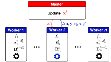
Figure 1: Asynchronous communication scheme used by the proposed algorithm.

We define the aggregate Hessian approximation as

$${\mathbf{B}}^{t}:=\sum_{i=1}^{n}{\mathbf{B}}_{i}^{t}=\sum_{i=1}^{n}{\mathbf{B}}_{i}^{t-d_{i}^{t}}$$ (6)

where we used (5). In addition, we introduce

$${\mathbf{u}}^{t}:=\sum_{i=1}^{n}{\mathbf{B}}_{i}^{t}{\mathbf{z}}_{i}^{t}=\sum_{i=1}^{n}{\mathbf{B}}_{i}^{t-d_{i}^{t}}{\mathbf{z}}_{i}^{t-d_{i}^{t}},\quad{\mathbf{g}}^{t}:=\sum_{i=1}^{n}\nabla f_{i}({\mathbf{z}}_{i}^{t})=\sum_{i=1}^{n}\nabla f_{i}({\mathbf{z}}_{i}^{t-d_{i}^{t}})$$ (7)

as the aggregate Hessian-variable product and aggregate gradient respectively where we made use of the identities (4)–(5). All these vectors and matrices are only available at the master node since it requires access to the information of all the workers.

Given that at step $t+1$ only a single index $i_{t}$ is updated, using the identities (4)–(7), it follows that the master has the update rules

$${\mathbf{B}}^{t+1} ={\mathbf{B}}^{t}+\left({\mathbf{B}}_{i_{t}}^{t+1}-{\mathbf{B}}_{i_{t}}^{t}\right)={\mathbf{B}}^{t}+\left({\mathbf{B}}_{i_{t}}^{t}-{\mathbf{B}}_{i_{t}}^{t-d_{i}^{t}}\right),$$ (8)

$${\mathbf{u}}^{t+1} ={\mathbf{u}}^{t}+\left({\mathbf{B}}_{i_{t}}^{t+1}{\mathbf{z}}_{i_{t}}^{t+1}-{\mathbf{B}}_{i_{t}}^{t}{\mathbf{z}}_{i_{t}}^{t}\right)={\mathbf{u}}^{t}+\left({\mathbf{B}}_{i_{t}}^{t+1}{\mathbf{x}}^{t-d_{i_{t}}^{t}}-{\mathbf{B}}_{i_{t}}^{t-d_{i_{t}}^{t}}{\mathbf{x}}^{t-D_{i_{t}}^{t}}\right),$$ (9)

$${\mathbf{g}}^{t+1} ={\mathbf{g}}^{t}+\left(\nabla f_{i_{t}}({\mathbf{z}}_{i_{t}}^{t+1})-\nabla f_{i_{t}}({\mathbf{z}}_{i_{t}}^{t})\right)={\mathbf{g}}^{t}+\left(\nabla f_{i_{t}}({\mathbf{x}}^{t-d_{i_{t}}^{t}})-\nabla f_{i_{t}}({\mathbf{x}}^{t-D_{i_{t}}^{t}})\right).$$ (10)

We observe that, only ${\mathbf{B}}_{i_{t}}^{t+1}$ and $\nabla f_{i_{t}}({\mathbf{z}}_{i_{t}}^{t+1})=\nabla f_{i_{t}}({\mathbf{x}}^{t-d_{i_{t}}^{t}})$ are required to be computed at step $t+1$. The former is obtained by the standard BFGS rule applied to $f_{i}$ carried out by the worker $i_{t}$:

$${\mathbf{B}}_{i_{t}}^{t+1}={\mathbf{B}}_{i_{t}}^{t}+\frac{{\mathbf{y}}_{i_{t}}^{t+1}({\mathbf{y}}_{i_{t}}^{t+1})^{\top}}{\alpha^{t+1}}-\frac{{\mathbf{q}}_{i_{t}}^{t+1}({\mathbf{q}}_{i_{t}}^{t+1})^{\top}}{\beta^{t+1}}$$ (11)

with

$$\alpha^{t+1}\coloneqq({\mathbf{y}}_{i_{t}}^{t+1})^{\top}{\mathbf{s}}_{i_{t}}^{t+1}\quad{\mathbf{y}}_{i_{t}}^{t+1}\coloneqq{\mathbf{z}}_{i_{t}}^{t+1}-{\mathbf{z}}_{i_{t}}^{t}={\mathbf{x}}^{t-d_{i_{t}}^{t}}-{\mathbf{x}}^{t-D_{i_{t}}^{t}},$$ (12)

$${\mathbf{q}}_{i_{t}}^{t+1}\coloneqq{\mathbf{B}}_{i_{t}}^{t}{\mathbf{s}}_{i_{t}}^{t+1},\quad\beta^{t+1}\coloneqq({\mathbf{s}}_{i_{t}}^{t+1})^{\top}{\mathbf{B}}_{i_{t}}^{t}{\mathbf{s}}_{i_{t}}^{t+1}=({\mathbf{s}}_{i_{t}}^{t+1})^{\top}{\mathbf{q}}_{i_{t}}^{t+1}.$$ (13)

Then, the master computes the new iterate as ${\mathbf{x}}^{t+1}=({\mathbf{B}}^{t+1})^{-1}\left({\mathbf{u}}^{t+1}-{\mathbf{g}}^{t+1}\right)$ and sends it to worker $i_{t}$. For the rest of the workers, we update the time counter without changing the variables, so ${\mathbf{z}}_{i}^{t+1}={\mathbf{z}}_{i}^{t}$ and ${\mathbf{B}}_{i}^{t+1}={\mathbf{B}}_{i}^{t}$ for $i\neq i_{t}$. Although, updating the inverse ${\mathbf{B}}^{t})^{-1}$ may seem costly first glance, in fact it can be computed efficiently in ${\cal O}(p^{2})$ iterations, similar to standard implementations of the BFGS methods. More specifically, if we introduce a new matrix

$${\mathbf{U}}^{t+1}\coloneqq({\mathbf{B}}^{t})^{-1}-\frac{({\mathbf{B}}^{t})^{-1}{\mathbf{y}}_{i_{t}}^{t+1}{({\mathbf{y}}_{i_{t}}^{t+1})^{\top}}({\mathbf{B}}^{t})^{-1}}{({\mathbf{y}}_{i_{t}}^{t+1})^{\top}{\mathbf{s}}_{i_{t}}^{t+1}+({{\mathbf{y}}_{i_{t}}^{t})^{\top}}({\mathbf{B}}^{t})^{-1}{\mathbf{y}}_{i_{t}}^{t+1}},$$ (14)

then, by the Sherman-Morrison-Woodbury formula, we have the identity

$$({\mathbf{B}}^{t+1})^{-1}={\mathbf{U}}^{t+1}+\frac{\ \!{\mathbf{U}}^{t+1}({\mathbf{B}}_{i_{t}}^{t-d_{i_{t}}^{t}}{\mathbf{s}}_{i_{t}}^{t+1})({\mathbf{B}}_{i_{t}}^{t-d_{i_{t}}^{t}}{\mathbf{s}}_{i_{t}}^{t+1})^{T}{\mathbf{U}}^{t+1}}{({\mathbf{s}}_{i_{t}}^{t+1})^{T}{\mathbf{B}}_{i_{t}}^{t-d_{i_{t}}^{t}}{\mathbf{s}}_{i_{t}}^{t+1}\!-\!({\mathbf{B}}_{i_{t}}^{t-d_{i}^{t}}{\mathbf{s}}_{i_{t}}^{t+1})^{T}{\mathbf{U}}^{t+1}({\mathbf{B}}_{i_{t}}^{t-d_{i_{t}}^{t}}{\mathbf{s}}_{i_{t}}^{t+1})},$$ (15)

Therefore, if we already have $({\mathbf{B}}^{t})^{-1}$, it suffices to have only matrix vector products. If we denote ${\mathbf{v}}^{t+1}=({\mathbf{B}}^{t})^{-1}{\mathbf{y}}_{i_{t}}^{t+1}$ and ${\mathbf{w}}^{t+1}\coloneqq{\mathbf{U}}^{t+1}{\mathbf{q}}_{i_{t}}^{t+1}$, then these equations can be simplified as

$${\mathbf{U}}^{t+1} =({\mathbf{B}}^{t})^{-1}-\frac{{\mathbf{v}}^{t+1}({\mathbf{v}}^{t+1})^{\top}}{\alpha^{t+1}+({\mathbf{v}}^{t+1})^{\top}{\mathbf{y}}_{i_{t}}^{t+1}},\quad{\mathbf{v}}^{t+1}=({\mathbf{B}}^{t})^{-1}{\mathbf{y}}_{i_{t}}^{t+1},$$ (16)

$$({\mathbf{B}}^{t+1})^{-1} ={\mathbf{U}}^{t+1}+\frac{{\mathbf{w}}^{t+1}({\mathbf{w}}^{t+1})^{\top}}{\beta^{t+1}-({\mathbf{q}}^{t+1})^{\top}{\mathbf{w}}^{t+1}},\quad{\mathbf{w}}^{t+1}\coloneqq{\mathbf{U}}^{t+1}{\mathbf{q}}_{i_{t}}^{t+1},$$ (17)

Algorithm 1 DAve-QN (implementation)

       If a worker sends an update:
Receive $\Delta{\mathbf{u}}$, ${\mathbf{y}}$, ${\mathbf{q}}$, $\alpha$, $\beta$ from it
${\mathbf{u}}={\mathbf{u}}+\Delta{\mathbf{u}}$, ${\mathbf{g}}={\mathbf{g}}+{\mathbf{y}}$, ${\mathbf{v}}=({\mathbf{B}})^{-1}{\mathbf{y}}$
${\mathbf{U}}=({\mathbf{B}})^{-1}-\frac{{\mathbf{v}}{\mathbf{v}}^{\top}}{\alpha+{\mathbf{v}}^{\top}{\mathbf{y}}}$
${\mathbf{w}}={\mathbf{U}}{\mathbf{q}}$, $({\mathbf{B}})^{-1}={\mathbf{U}}+\frac{{\mathbf{w}}{\mathbf{w}}^{\top}}{\beta-{\mathbf{q}}^{\top}{\mathbf{w}}}$
${\mathbf{x}}=({\mathbf{B}})^{-1}({\mathbf{u}}-{\mathbf{g}})$
Send ${\mathbf{x}}$ to the worker in return

end for

Interrupt all workers
Output ${\mathbf{x}}^{T}$

       Receive ${\mathbf{x}}$
${\mathbf{s}}_{i}={\mathbf{x}}-{\mathbf{z}}_{i}$
${\mathbf{y}}_{i}=\nabla f_{i}({\mathbf{x}})-\nabla f_{i}({\mathbf{z}}_{i})$
${\mathbf{q}}_{i}={\mathbf{B}}_{i}{\mathbf{s}}_{i}$
$\alpha={\mathbf{y}}_{i}^{\top}{\mathbf{s}}_{i}$
$\beta={\mathbf{s}}_{i}^{\top}{\mathbf{B}}_{i}^{t}{\mathbf{s}}_{i}$
${\mathbf{u}}={\mathbf{B}}_{i}{\mathbf{z}}_{i}$
${\mathbf{B}}_{i}={\mathbf{B}}_{i}+\frac{{\mathbf{y}}_{i}{\mathbf{y}}_{i}^{\top}}{\alpha}-\frac{{\mathbf{q}}_{i}{\mathbf{q}}_{i}^{\top}}{\beta}$
$\Delta{\mathbf{u}}={\mathbf{B}}_{i}{\mathbf{x}}-{\mathbf{u}}$
${\mathbf{z}}_{i}={\mathbf{x}}$
Send $\Delta{\mathbf{u}},{\mathbf{y}}_{i},{\mathbf{q}}_{i},\alpha,\beta$ to the master

end while

where $\alpha^{t+1},\beta^{t+1},{\mathbf{q}}_{i_{t}}^{t+1}$ and ${\mathbf{y}}_{i_{t}}^{t+1}$ are defined by (12)–(13).

The steps of the DAve-QN at the master node and the workers are summarized in Algorithm 1. Note that steps at worker $i$ is devoted to performing the update in (11). Using the computed matrix ${\mathbf{B}}_{i}$, node $i$ evaluates the vector $\Delta{\mathbf{u}}$. Then, it sends the vectors $\Delta{\mathbf{u}}$, ${\mathbf{y}}_{i}$, and ${\mathbf{q}}_{i}$ as well as the scalars $\alpha$ and $\beta$ to the master node. The master node uses the variation vectors $\Delta{\mathbf{u}}$ and ${\mathbf{y}}$ to update ${\mathbf{u}}$ and ${\mathbf{g}}$. Then, it performs the update ${\mathbf{x}}^{t+1}=({\mathbf{B}}^{t+1})^{-1}\left({\mathbf{u}}^{t+1}-{\mathbf{g}}^{t+1}\right)$ by following the efficient procedure presented in (16)–(17). A more detailed version of Algorithm 1 with exact indices is presented in the supplementary material.

We define epochs $\{T_{m}\}_{m}$ by setting $T_{1}=0$ and the following recursion:

$$T_{m+1} =\min\{t:\text{ each machine made at least 2 updates on the interval }[T_{m},t]\}$$

$$=\min\{t:t-D_{i}^{t}\geq T_{m}\text{ for all }i=1,..,M\}.$$

The proof of the following simple lemma is provided in the supplementary material.

Lemma 1.

Algorithm 2 iterates satisfy ${\mathbf{x}}^{t}=\left(\frac{1}{n}\sum_{i=1}^{n}{\mathbf{B}}_{i}^{t}\right)^{-1}\left(\frac{1}{n}\sum_{i=1}^{n}{\mathbf{B}}_{i}^{t}{\mathbf{z}}_{i}^{t}-\frac{1}{n}\sum_{i=1}^{n}\nabla f_{i}({\mathbf{z}}_{i}^{t})\right)$.

The result in Lemma 1 shows that explicit relationship between the updated variable ${\mathbf{x}}^{t}$ based on the proposed DAve-QN and the local information at the workers. We will use this update to analyze DAve-QN.

Proposition 1 (Epochs’ properties).

The following relations between epochs and delays hold:

• For any $t\in[T_{m+1},T_{m+2})$ and any $i=1,2,\dots,n$ one has $t-D_{i}^{t}\in[T_{m},t)$.

• If delays are uniformly bounded, i.e. there exists a constant $d$ such that $d_{i}^{t}\leq d$ for all $i$ and $t$, then for all $m$ we have $T_{m+1}-T_{m}\leq D\coloneqq 2d+1$ and $T_{m}\leq Dm$.

• If we define average delays as $\overline{d^{t}}\coloneqq\tfrac{1}{n}\sum_{i=1}^{n}d_{i}^{t}$, then $\overline{d^{t}}\geq(n-1)/2$. Moreover, assuming that $\overline{d^{t}}\leq(n-1)/2+\overline{d}$ for all $t$, we get $T_{m}\leq 4n(\overline{d}+1)m$.

Clearly, without visiting every function we can not converge to ${\mathbf{x}}^{*}$. Therefore, it is more convenient to measure performance in terms of number of passed epochs, which can be considered as our alternative counter for time. Proposition 1 explains how one can get back to the iterations time counter assuming that delays are bounded uniformly or on average. However, uniform upper bounds are rather pessimistic which motivates the convergence in epochs that we consider.

3 Convergence Analysis

In this section, we study the convergence properties of the proposed distributed asynchronous quasi-Newton method. To do so, we first assume that the following conditions are satisfied.

Assumption 1.

The component functions $f_{i}$ are $L$-smooth and $\mu$-strongly convex, i.e., there exist positive constants $0<\mu\leq L$ such that, for all $i$ and ${\mathbf{x}},{\hat{\mathbf{x}}}\in{\mathbb{R}}^{p}$

$$\mu\|{\mathbf{x}}-{\hat{\mathbf{x}}}\|^{2}\leq(\nabla f_{i}({\mathbf{x}})-\nabla f_{i}({\hat{\mathbf{x}}}))^{T}({\mathbf{x}}-{\hat{\mathbf{x}}})\leq L\|{\mathbf{x}}-{\hat{\mathbf{x}}}\|^{2}.$$ (18)

Assumption 2.

The Hessians $\nabla^{2}f_{i}$ are Lipschitz contunuous, i.e., there exists a positive constant $\tilde{L}$ such that, for all $i$ and ${\mathbf{x}},{\hat{\mathbf{x}}}\in{\mathbb{R}}^{p}$, we can write $\|\nabla^{2}f_{i}({\mathbf{x}})-\nabla^{2}f_{i}({\hat{\mathbf{x}}})\|\leq\tilde{L}\|{\mathbf{x}}-{\hat{\mathbf{x}}}\|$.

It is well-known and widely used in the literature on Newton’s and quasi-Newton methods [47, 46, 48, 49] that if the function $f_{i}$ has Lipschitz continuous Hessian $x\mapsto\nabla^{2}f_{i}(x)$ with parameter $\tilde{L}$ then

$$\left\|\nabla^{2}f_{i}({\tilde{\mathbf{x}}})({\mathbf{x}}-{\hat{\mathbf{x}}})-(\nabla f_{i}({\mathbf{x}})-\nabla f_{i}({\hat{\mathbf{x}}}))\right\|\leq{\tilde{L}}\|{\mathbf{x}}-{\hat{\mathbf{x}}}\|\max\left\{\|{\mathbf{x}}-{\tilde{\mathbf{x}}}\|,\|{\hat{\mathbf{x}}}-{\tilde{\mathbf{x}}}\|\right\},$$ (19)

for any arbitrary ${\mathbf{x}},{\tilde{\mathbf{x}}},{\hat{\mathbf{x}}}\in{\mathbb{R}}^{p}$. See, for instance, Lemma 3.1 in [46].

Lemma 2.

Consider the Dave-QN algorithm summarized in Algorithm 2. For any $i$, define the residual sequence for function $f_{i}$ as $\sigma_{i}^{t}:=\max\{\|{\mathbf{z}}_{i}^{t}-{\mathbf{x}}^{*}\|,\|{\mathbf{z}}_{i}^{t-D_{i}^{t}}-{\mathbf{x}}^{*}\|\}$ and set ${\mathbf{M}}_{i}=\nabla^{2}f_{i}({\mathbf{x}}^{*})^{-1/2}$. If Assumptions 1 and 2 hold and the condition $\sigma_{i}^{t}<\mu/(3\tilde{L})$ is satisfied then a Hessian approximation matrix ${\mathbf{B}}_{i}^{t}$ and its last updated version ${\mathbf{B}}_{i}^{t-D_{i}^{t}}$ satisfy

$$\left\|{\mathbf{B}}_{i}^{t}\!-\!\nabla^{2}f_{i}({\mathbf{x}}^{*})\right\|_{{\mathbf{M}}_{i}}\leq\!\left[\left[1\!-\!\alpha{\theta_{i}^{t-D_{i}^{t}}}^{2}\right]^{\frac{1}{2}}\!\!\!+\alpha_{3}\sigma_{i}^{t-D_{i}^{t}}\right]\!\!\left\|{\mathbf{B}}_{i}^{t-D_{i}^{t}}-\nabla^{2}f_{i}({\mathbf{x}}^{*})\right\|_{{\mathbf{M}}_{i}}\!\!+\!\alpha_{4}\sigma_{i}^{t-D_{i}^{t}},$$ (20)

where $\alpha,\alpha_{3}$, and $\alpha_{4}$ are some positive constants and $\theta_{i}^{t-D_{i}^{t}}=\frac{\|{\mathbf{M}}_{i}({\mathbf{B}}_{i}^{t-D_{i}^{t}}-\nabla^{2}f_{i}({\mathbf{x}}^{*})){\mathbf{s}}_{i}^{t-D_{i}^{t}}\|}{\|{\mathbf{B}}_{i}^{t-D_{i}^{t}}-\nabla^{2}f_{i}({\mathbf{x}}^{*})\|_{{\mathbf{M}}_{i}}\|{\mathbf{M}}_{i}^{-1}{\mathbf{s}}_{i}^{t-D_{i}^{t}}\|}$ with the convention that $\theta_{i}^{t-D_{i}^{t}}=0$ in the special case ${\mathbf{B}}_{i}^{t-D_{i}^{t}}=\nabla^{2}f_{i}({\mathbf{x}}^{*})$.

Lemma 2 shows that, if we neglect the additive term $\alpha_{4}\sigma_{i}^{t-D_{i}^{t}}$ in (20), the difference between the Hessian approximation matrix ${\mathbf{B}}_{i}^{t}$ for the function $f_{i}$ and its corresponding Hessian at the optimal point $\nabla^{2}f_{i}({\mathbf{x}}^{*})$ decreases by following the update of Algorithm 2. To formalize this claim and show that the additive term is negligible, we prove in the following lemma that the sequence of errors $\|{\mathbf{x}}^{t}-{\mathbf{x}}^{*}\|$ converges to zero R-linearly which also implies linear convergence of the sequence $\sigma_{i}^{t}$.

Lemma 3.

Consider the Dave-QN method outlined in Algorithm 2. Further assume that the conditions in Assumptions 1 and 2 are satisfied. Then, for any $r\in(0,1)$ there exist positive constants $\epsilon(r)$ and $\delta(r)$ such that if $\|{\mathbf{x}}^{0}-{\mathbf{x}}^{*}\|<\epsilon(r)$ and $\|{\mathbf{B}}_{i}^{0}-\nabla^{2}f_{i}({\mathbf{x}}^{*})\|_{\mathbf{M}}<\delta(r)$ for ${\mathbf{M}}=\nabla^{2}f_{i}({\mathbf{x}}^{*})^{-1/2}$ and $i=1,2,\dots,n$, the sequence of iterates generated by DAve-QN satisfy $\|{\mathbf{x}}^{t}-{\mathbf{x}}^{*}\|\leq r^{m}\|{\mathbf{x}}^{0}-{\mathbf{x}}^{*}\|$ for all $t\in[T_{m},T_{m+1})$.

The result in Lemma 3 shows that the error for the sequence of iterates generated by the Dave-QN method converge to zero at least linearly in a neighborhood of the optimal solution. Using this result, in the following theorem we prove our main result, which shows a specific form of superlinear convergence.

Theorem 1.

Consider the proposed method outlined in Algorithm 2. Suppose that Assumptions 1 and 2 hold. Further, assume that the required conditions for the results in Lemma 2 and Lemma 3 are satisfied. Then, the sequence of residuals $\|{\mathbf{x}}^{t}-{\mathbf{x}}^{*}\|$ satisfies $\lim_{t\rightarrow\infty}\frac{\max_{t\in[T_{m+1},T_{m+2})}\|{\mathbf{x}}^{t}-{\mathbf{x}}^{*}\|}{\max_{t\in[T_{m},T_{m+1})}\|{\mathbf{x}}^{t}-{\mathbf{x}}^{*}\|}=0$.

The result in Theorem 1 shows that the maximum residual in an epoch divided by the the maximum residual for the previous epoch converges to zero. This observation shows that there exists a subsequence of residuals $\|{\mathbf{x}}^{t}-{\mathbf{x}}^{*}\|$ that converges to zero superlinearly.

4 Experiments

We conduct our experiments on five datasets (epsilon, SUSY, covtype, mnist8m, cifar10) from the LIBSVM library [50]. For the first three datasets, the objective considered is a binary logistic regression problem $f(x)=\frac{1}{n}\sum_{i=1}^{n}\log(1+\exp(-b_{i}a_{i}^{T}x)+\frac{\lambda}{2}\|x\|^{2}$ where $a_{i}\in\mathbb{R}^{p}$ are the feature vectors and $b_{i}\in\{-1,+1\}$ are the labels. The other two datasets are about multi-class classification instead of binary classification. For comparison, we used two other algorithms designed for distributed optimization:

• Distributed Average Repeated Proximal Gradient (DAve-RPG) [39]. It is a recently proposed competitive state-of-the-art asynchronous method for first-order distributed optimization, numerically demonstrated to outperform incremental aggregated gradient methods [6, 38] and synchronous proximal gradient methods in [39].

• Distributed Approximate Newton (DANE) [24]. This is a well-known Newton-like method that does not require a parameter server node, but performs reduce operations at every step.

In the experiments we did not implement algorithms that require shared memory (such as ASAGA [11] or Hogwild! [2]) because in our setting of master/worker communication model, the memory is not shared. Since the focus of this paper is mainly on asynchronous algorithms where the communication delays is the main bottleneck, for fairness reasons, we are also not comparing our method with some synchronous algorithms such as DISCO [26] that would not support asynchronous computations. Our code is publicly available at https://github.com/DAve-QN/source.

The experiments are conducted on XSEDE Comet CPUs (Intel Xeon E5-2680v3 2.5 GHz). For DAVE-QN and DAVE-RPG we build a cluster of 17 processes in which 16 of the processes are workers and one is the master. The DANE method does not require a master so we use 16 workers for its experiments. We split the data randomly among the processes so that each has the same amount of samples. In our experiments, Intel MKL 11.1.2 and MVAPICH2/2.1 are used for the BLAS (sparse/dense) operations and we use MPI programming compiled with mpicc 14.0.2. Each experiment is repeated thirty times and the average is reported.

For the methods’ parameters the best options provided by the method authors are used. For DAve-RPG the stepsize $\tfrac{1}{L}$ is used where $L$ is found by a standard backtracking line search similar to [51]. DANE has two parameters, $\eta$ and $\mu$. As recommended by the authors, we use $\eta=1$ and $\mu=3\lambda$. We tuned $\lambda$ to the dataset, choosing $\lambda=1$ for the mnist8m and cifar10 datasets, $\lambda=0.001$ for the epsilon and SUSY and $\lambda=0.1$ for the covtype. Since DANE requires a local optimization problem to be solved, we use SVRG [52] as its local solver where its parameters are selected based on the experiments in [24].

Our results are summarized in Figure 2 where we report the expected suboptimality versus time in a logarithmic y-axis. For linearly convergent algorithms, the slope of this plot determines the convergence rate. DANE method is the slowest on these datasets, but it does not need a master, therefore it can apply to multi-agent applications [44] where master nodes are often not available. We observe that Dave-QN performs significantly better on all the datasets except cifar10, illustrating the superlinear convergence behavior provided by our theory compared to other methods. For the cifar10 dataset, $p$ is the largest. Although Dave-QN starts faster than Dave-RPG , Rave-RPG has a cheaper iteration complexity ($O(p)$ compared to $O(p^{2})$ of Dave-QN) and becomes eventually faster.

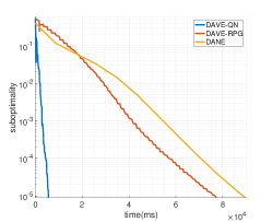
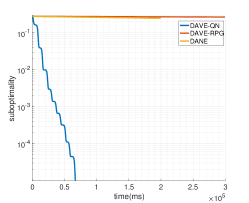
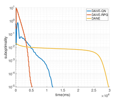
mnist8m $(p=784,n=8.1M)$	epsilon $(p=2000,n=500K)$	cifar10 $(p=3072,n=60K)$

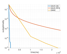
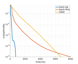
SUSY $(p=19,n=5M)$	covtype $(p=54,n\approx 2.9M)$

Figure 2: Expected suboptimality versus time.

5 Conclusion and Future Work

In this paper, we focused on the problem of minimizing a large-scale empirical risk minimization in a distributed manner. We used an asynchronous architecture which requires no global coordination between the master node and the workers. Unlike distributed first-order methods that follow the gradient direction to update the iterates, we proposed a distributed averaged quasi-Newton (DAve-QN) algorithm that uses a quasi-Newton approximate Hessian of the workers’ local objective function to update the decision variable. In contrast to second-order methods that require computation of the local functions Hessians, the proposed DAve-QN only uses gradient information to improve the convergence of first-order methods in ill-conditioned settings. It is worth mentioning that the computational cost of each iteration of DAve-QN is $\mathcal{O}(p^{2})$, while the size of the vectors that are communicated between the master and workers is $\mathcal{O}(p)$. Our theoretical results show that the sequence of iterates generated at the master node by following the update of DAve-QN converges superlinearly to the optimal solution when the objective functions at the workers are smooth and strongly convex. Our results hold for both bounded delays and unbounded delays with a bounded time-average. Numerical experiments illustrate the performance of our method.

The choice of the stepsize in the initial stages of the algorithm is the key to get good overall iteration complexity for second-order methods. Investigating several line search techniques developed for BFGS and adapting it to the distributed asynchronous setting is a future research direction of interest. Another promising direction would be developing Newton-like methods that can go beyond superlinear convergence while preserving communication complexity. Finally, investigating the dependence of the convergence properties on the sample size $m_{i}$ of each machine $i$ would be interesting, in particular one would expect the performance in terms of communication complexity to improve if the sample size of each machine is increased.

Acknowledgments

This work was supported in part by the grants NSF DMS-1723085, NSF CCF-1814888 and NSF CCF-1657175. This work used the Extreme Science and Engineering Discovery Environment (XSEDE) [53], which is supported by National Science Foundation grant number ACI-1548562.

Appendix A Supplementary Material

A.1 The proposed DAve-QN method with exact time indices

Algorithm 2 DAve-QN with comprehensive notations)

       If a worker sends an update:
Receive $\Delta{\mathbf{u}}^{t}$, ${\mathbf{y}}$, ${\mathbf{q}}$, $\alpha^{t}$, $\beta^{t}$ from it
${\mathbf{u}}^{t}={\mathbf{u}}^{t-1}+\Delta{\mathbf{u}}^{t}$
${\mathbf{g}}^{t}={\mathbf{g}}^{t-1}+{\mathbf{y}}$
${\mathbf{v}}^{t}=({\mathbf{B}}^{t-1})^{-1}{\mathbf{y}}$
${\mathbf{U}}^{t}=({\mathbf{B}}^{t-1})^{-1}-\frac{{\mathbf{v}}^{t}{\mathbf{v}}^{t\top}}{\alpha^{t}+{\mathbf{v}}{t\top}{\mathbf{y}}}$
${\mathbf{w}}^{t}={\mathbf{U}}^{t}{\mathbf{q}}$
$({\mathbf{B}}^{t})^{-1}={\mathbf{U}}^{t}+\frac{{\mathbf{w}}^{t}{\mathbf{w}}^{t\top}}{\beta^{t}-{\mathbf{q}}^{T}{\mathbf{w}}^{t}}$
${\mathbf{x}}^{t}=({\mathbf{B}}^{t})^{-1}({\mathbf{u}}^{t}-{\mathbf{g}}^{t})$
Send ${\mathbf{x}}^{t}$ to the slave in return

end for

Interrupt all slaves
Output ${\mathbf{x}}^{T}$

       Receive ${\mathbf{x}}^{t-D_{i}^{t}}$ at moment $t-D_{i}^{t}$
Perform below steps by moment $t-d_{i}^{t}$
${\mathbf{z}}_{i}^{t}={\mathbf{z}}_{i}^{t-d_{i}^{t}}={\mathbf{x}}^{t-D_{i}^{t}}$
${\mathbf{s}}_{i}^{t}={\mathbf{s}}_{i}^{t-d_{i}^{t}}={\mathbf{z}}^{t-d_{i}^{t}}-{\mathbf{z}}_{i}^{t-D_{i}^{t}}$
${\mathbf{y}}_{i}^{t}={\mathbf{y}}_{i}^{t-d_{i}^{t}}=\nabla f_{i}({\mathbf{x}}^{t-d_{i}^{t}})-\nabla f_{i}({\mathbf{z}}_{i}^{t})$
${\mathbf{q}}_{i}^{t}={\mathbf{q}}_{i}^{t-d_{i}^{t}}={\mathbf{B}}_{i}^{t-D_{i}^{t}}{\mathbf{s}}_{i}^{t-d_{i}^{t}}$
$\alpha^{t-d_{i}^{t}}={\mathbf{y}}_{i}^{tT}{\mathbf{s}}_{i}^{t}$
$\beta^{t-d_{i}^{t}}=({\mathbf{s}}_{i}^{t-d_{i}^{t}})^{T}{\mathbf{B}}_{i}^{t-D_{i}^{t}}{\mathbf{s}}_{i}^{t}$
${\mathbf{B}}_{i}^{t-d_{i}^{t}}={\mathbf{B}}_{i}^{t-D_{i}^{t}}+\frac{{\mathbf{y}}_{i}^{t}{\mathbf{y}}_{i}^{tT}}{\alpha^{t-d_{i}^{t}}}-\frac{{\mathbf{q}}_{i}^{t}{\mathbf{q}}_{i}^{tT}}{\beta^{t-d_{i}^{t}}}$
$\Delta{\mathbf{u}}^{t-d_{i}^{t}}={\mathbf{B}}_{i}^{t-d_{i}^{t}}{\mathbf{z}}_{i}^{t-d_{i}^{t}}-{\mathbf{B}}_{i}^{t-D_{i}^{t}}{\mathbf{z}}_{i}^{t-D_{i}^{t}}$
Send $\Delta{\mathbf{u}}^{t-d_{i}^{t}},{\mathbf{y}}_{i}^{t-d_{i}^{t}},{\mathbf{q}}_{i}^{t-d_{i}^{t}},\alpha^{t-d_{i}^{t}},\beta^{t-d_{i}^{t}}$ to the master at moment $t-d_{i}^{t}$

end while

A.2 Proof of Lemma 1

Proof.

To verify the claim, we need to show that ${\mathbf{u}}^{t}=\sum_{i=1}^{n}{\mathbf{B}}_{i}^{t}{\mathbf{z}}_{i}^{t}$ and ${\mathbf{g}}^{t}=\sum_{i=1}^{n}\nabla f_{i}({\mathbf{z}}_{i}^{t})$. They follow from our delayed vectors notation ${\mathbf{z}}_{i}^{t}={\mathbf{z}}_{i}^{t-d_{i}^{t}}$ and how $\Delta{\mathbf{u}}^{t-d_{i}^{t}}$ and ${\mathbf{y}}_{i}^{t-d_{i}^{t}}$ are computed by the corresponding worker. ∎

A.3 Proof of Lemma 2

To prove the claim in Lemma 2 we first prove the following intermediate lemma using the result of Lemma 5.2 in [46].

Lemma 4.

Consider the proposed method outlined in Algorithm 2. Let ${\mathbf{M}}$ be a nonsingular symmetric matrix such that

$$\|{\mathbf{M}}{\mathbf{y}}_{i}^{t}-{\mathbf{M}}^{-1}{\mathbf{s}}_{i}^{t}\|\leq\beta\|{\mathbf{M}}^{-1}{\mathbf{s}}_{i}^{t}\|,$$ (21)

for some $\beta\in[0,1/3]$ and vectors ${\mathbf{s}}_{i}^{t}$ and ${\mathbf{y}}_{i}^{t}$ in ${\mathbb{R}}^{p}$ with ${\mathbf{s}}_{i}^{t}\neq{\mathbf{0}}$. Let’s denote $i$ as the index that has been updated at time $t$. Then, there exist positive constants $\alpha$, $\alpha_{1}$, and $\alpha_{2}$ such that, for any symmetric ${\mathbf{A}}\in{\mathbb{R}}^{p\times p}$ we have,

$$\|{\mathbf{B}}_{i}^{t}-{\mathbf{A}}\|_{\mathbf{M}} \leq\left[(1-\alpha\theta^{2})^{1/2}+\alpha_{1}\frac{\|{\mathbf{M}}{\mathbf{y}}_{i}^{t-D_{i}^{t}}-{\mathbf{M}}^{-1}{\mathbf{s}}_{i}^{t-D_{i}^{t}}\|}{\|{\mathbf{M}}^{-1}{\mathbf{s}}_{i}^{t-D_{i}^{t}}\|}\right]\|{\mathbf{B}}_{i}^{t-D_{i}^{t}}-{\mathbf{A}}\|_{\mathbf{M}}$$

$$\quad+\alpha_{2}\frac{\|{\mathbf{y}}_{i}^{t-D_{i}^{t}}-{\mathbf{A}}{\mathbf{s}}_{i}^{t-D_{i}^{t}}\|}{\|{\mathbf{M}}^{-1}{\mathbf{s}}_{i}^{t-D_{i}^{t}}\|},$$ (22)

where $\alpha=(1-2\beta)/(1-\beta^{2})\in[3/8,1]$, $\alpha_{1}=2.5(1-\beta)^{-1}$, $\alpha_{2}=2(1+2\sqrt{p})\|{\mathbf{M}}\|_{\mathbf{F}}$, and

$$\theta=\frac{\|{\mathbf{M}}({\mathbf{B}}_{i}^{t-D_{i}^{t}}-{\mathbf{A}}){\mathbf{s}}_{i}^{t-D_{i}^{t}}\|}{\|{\mathbf{B}}_{i}^{t-D_{i}^{t}}-{\mathbf{A}}\|_{\mathbf{M}}\|{\mathbf{M}}^{-1}{\mathbf{s}}_{i}^{t-D_{i}^{t}}\|}\quad\text{for}\ {\mathbf{B}}_{i}^{t-D_{i}^{t}}\neq{\mathbf{A}},\qquad\theta=0\quad\text{for}\ {\mathbf{B}}_{i}^{t-D_{i}^{t}}={\mathbf{A}}.$$ (23)

Proof.

By definition of delays $d_{i}^{t}$, the function $f_{i}$ was updated at step $t-d_{i}^{t}$ and ${\mathbf{B}}_{i}^{t-1}$ is equal to ${\mathbf{B}}_{i}^{t-D_{i}^{t}}$. Considering this observation and the result of Lemma 5.2 in [46], the claim follows. ∎

Note that the result in Lemma 4 characterizes an upper bound on the difference between the Hessian approximation matrices ${\mathbf{B}}_{i}^{t}$ and ${\mathbf{B}}_{i}^{t-D_{i}^{t}}$ and any positive definite matrix ${\mathbf{A}}$. Let us show that matrices ${\mathbf{M}}=\nabla^{2}f_{i}({\mathbf{x}}^{*})^{-1/2}$ and ${\mathbf{A}}=\nabla^{2}f_{i}({\mathbf{x}}^{*})$ satisfy the conditions of Lemma 4. By strong convexity of $f_{i}$ we have $\|\nabla^{2}f_{i}({\mathbf{x}}^{*})^{1/2}{\mathbf{s}}_{i}^{t-D_{i}^{t}}\|\geq\sqrt{\mu}\|{\mathbf{s}}_{i}^{t-D_{i}^{t}}\|$. Combined with Assumption 2, it gives that

$$\frac{\|{\mathbf{y}}_{i}^{t-D_{i}^{t}}-\nabla^{2}f_{i}({\mathbf{x}}^{*}){\mathbf{s}}_{i}^{t-D_{i}^{t}}\|}{\|\nabla^{2}f_{i}({\mathbf{x}}^{*})^{1/2}{\mathbf{s}}_{i}^{t-D_{i}^{t}}\|}\leq\frac{\tilde{L}\|{\mathbf{s}}_{i}^{t-D_{i}^{t}}\|\max\{\|{\mathbf{z}}_{i}^{t-D_{i}^{t}}-{\mathbf{x}}^{*}\|,\|{\mathbf{z}}_{i}^{t}-{\mathbf{x}}^{*}\|\}}{\sqrt{\mu}\|{\mathbf{s}}_{i}^{t-D_{i}^{t}}\|}=\frac{\tilde{L}}{\sqrt{\mu}}\sigma_{i}^{t}$$ (24)

This observation implies that the left hand side of the condition in (21) for ${\mathbf{M}}=\nabla^{2}f_{i}({\mathbf{x}}^{*})^{-1/2}$ is bounded above by

$$\frac{\|{\mathbf{M}}{\mathbf{y}}_{i}^{t-D_{i}^{t}}-{\mathbf{M}}^{-1}{\mathbf{s}}_{i}^{t-D_{i}^{t}}\|}{\|{\mathbf{M}}^{-1}{\mathbf{s}}_{i}^{t-D_{i}^{t}}\|}\leq\frac{\|\nabla^{2}f_{i}({\mathbf{x}}^{*})^{-1/2}\|\|{\mathbf{y}}_{i}^{t-D_{i}^{t}}-\nabla^{2}f_{i}({\mathbf{x}}^{*}){\mathbf{s}}_{i}^{t-D_{i}^{t}}\|}{\|\nabla^{2}f_{i}({\mathbf{x}}^{*})^{1/2}{\mathbf{s}}_{i}^{t-D_{i}^{t}}\|}\leq\frac{\tilde{L}}{\mu}\sigma_{i}^{t}$$ (25)

Thus, the condition in (21) is satisfied since $\tilde{L}\sigma_{i}^{t}/\mu<1/3.$ Replacing the upper bounds in (24) and (25) into the expression in (4) implies the claim in (20) with

$$\beta=\frac{\tilde{L}}{\mu}\sigma_{i}^{t},\ \alpha=\frac{1-2\beta}{1-\beta^{2}},\ \alpha_{3}=\frac{5\tilde{L}}{2\mu(1-\beta)},\ \alpha_{4}=\frac{{2(1+2\sqrt{p})\tilde{L}}}{\sqrt{\mu}}\|\nabla^{2}f_{i}({\mathbf{x}}^{*})^{-\frac{1}{2}}\|_{\mathbf{F}},$$ (26)

and the proof is complete.

A.4 Proof of Lemma 3

We first state the following result from Lemma 6 in [32], which shows an upper bound for the error $\|{\mathbf{x}}^{t}-{\mathbf{x}}^{*}\|$ in terms of the gap between the delayed variables ${\mathbf{z}}_{i}^{t}$ and the optimal solution ${\mathbf{x}}^{*}$ and the difference between the Newton direction $\nabla^{2}f_{i}({\mathbf{x}}^{*})\left({\mathbf{z}}_{i}^{t}-{\mathbf{x}}^{*}\right)$ and the proposed quasi-Newton direction ${\mathbf{B}}_{i}^{t}\left({\mathbf{z}}_{i}^{t}-{\mathbf{x}}^{*}\right)$.

Lemma 5.

If Assumptions 1 and 2 hold, then the sequence of iterates generated by Algorithm 2 satisfies

$$\|{\mathbf{x}}^{t}-{\mathbf{x}}^{*}\|\leq\frac{\tilde{L}\Gamma^{t}}{n}\sum_{i=1}^{n}\left\|{\mathbf{z}}_{i}^{t}-{\mathbf{x}}^{*}\right\|^{2}+\frac{\Gamma^{t}}{n}\sum_{i=1}^{n}\left\|\left({\mathbf{B}}_{i}^{t}-\nabla^{2}f_{i}({\mathbf{x}}^{*})\right)\left({\mathbf{z}}_{i}^{t}-{\mathbf{x}}^{*}\right)\right\|,$$ (27)

where $\Gamma^{t}:=\|((1/n)\sum_{i=1}^{n}{\mathbf{B}}_{i}^{t})^{-1}\|$.

We use the result in Lemma 5 to prove the claim of Lemma 3. We will prove the claimed convergence rate in Lemma 3together with an additional claim

$$\left\|{\mathbf{B}}_{i}^{t}-\nabla^{2}f_{i}({\mathbf{x}}^{*})\right\|_{\mathbf{M}}\leq 2\delta$$

by inductions on $m$ and on $t\in[T_{m},T_{m+1})$. The base case of our induction is $m=0$ and $t=0$, which is the initialization step, so let us start with it.

Since all norms in finite dimensional spaces are equivalent, there exists a constant $\eta>0$ such that $\|{\mathbf{A}}\|\leq\eta\|{\mathbf{A}}\|_{\mathbf{M}}$ for all ${\mathbf{A}}$. Define $\gamma\coloneqq 1/\mu$ and $d\coloneqq\max_{m}(T_{m+1}-T_{m})$, and assume that $\epsilon(r)=\epsilon$ and $\delta(r)=\delta$ are chosen such that

$$(2\alpha_{3}\delta+\alpha_{4})\frac{d\epsilon}{1-r}\leq\delta\quad\text{and}\quad\gamma(1+r)[\tilde{L}\epsilon+2\eta\delta]\leq r,$$ (28)

where $\alpha_{3}$ and $\alpha_{4}$ are the constants from Lemma 2. As $\|{\mathbf{B}}_{i}^{0}-\nabla^{2}f_{i}({\mathbf{x}}^{*})\|_{\mathbf{M}}\leq\delta$, we also have

$$\|{\mathbf{B}}_{i}^{0}-\nabla^{2}f_{i}({\mathbf{x}}^{*})\|\leq\eta\delta.$$

Therefore, by triangle inequality from $\|\nabla^{2}f_{i}({\mathbf{x}}^{*})\|\leq L$ we obtain $\|{\mathbf{B}}_{i}^{0}\|\leq\eta\delta+L$, so $\|(1/n)\sum_{i=1}^{n}{\mathbf{B}}_{i}^{0}\|\leq\eta\delta+L$. The second part of inequality (28) also implies $2\gamma(1+r)\eta\delta\leq r$. Moreover, it holds that $\|{\mathbf{B}}_{i}^{0}-\nabla^{2}f_{i}({\mathbf{x}}^{*})\|\leq\eta\delta<2\eta\delta$ and by Assumption 1 $\gamma\geq\|\nabla^{2}f_{i}({\mathbf{x}}^{*})^{-1}\|$, so we obtain by Banach Lemma that

$$\|({\mathbf{B}}_{i}^{0})^{-1}\|\leq(1+r)\gamma.$$

We formally prove this result in the following lemma.

Lemma 6.

If the Hessian approximation ${\mathbf{B}}_{i}$ satisfies the inequality $\|{\mathbf{B}}_{i}-\nabla^{2}f_{i}({\mathbf{x}}^{*})\|\leq 2\eta\delta$ and $\|\nabla^{2}f_{i}({\mathbf{x}}^{*})^{-1}\|\leq\gamma$, then we have $\|{\mathbf{B}}_{i}^{-1}\|\leq(1+r)\gamma.$

Proof.

Note that according to Banach Lemma, if a matrix ${\mathbf{A}}$ satisfies the inequality $\|{\mathbf{A}}-{\mathbf{I}}\|\leq 1$, then it holds $\|{\mathbf{A}}^{-1}\|\leq\frac{1}{1-\|{\mathbf{A}}-{\mathbf{I}}\|}$.

We first show that $\|\nabla^{2}f_{i}({\mathbf{x}}^{*})^{-1/2}{\mathbf{B}}_{i}\nabla^{2}f_{i}({\mathbf{x}}^{*})^{-1/2}-{\mathbf{I}}\|\leq 1$. To do so, note that

$$\|\nabla^{2}f_{i}({\mathbf{x}}^{*})^{-1/2}{\mathbf{B}}_{i}\nabla^{2}f_{i}({\mathbf{x}}^{*})^{-1/2}-{\mathbf{I}}\| \leq\|\nabla^{2}f_{i}({\mathbf{x}}^{*})^{-1/2}\|\|{\mathbf{B}}_{i}-\nabla^{2}f_{i}({\mathbf{x}}^{*})\|\|\nabla^{2}f_{i}({\mathbf{x}}^{*})^{-1/2}\|$$

$$\leq 2\eta\delta\gamma$$

$$\leq\frac{r}{r+1}$$

$$<1.$$ (29)

Now using this result and Banach Lemma we can show that

$$\|\nabla^{2}f_{i}({\mathbf{x}}^{*})^{1/2}{\mathbf{B}}_{i}^{-1}\nabla^{2}f_{i}({\mathbf{x}}^{*})^{1/2}\| \leq\frac{1}{1-\|\nabla^{2}f_{i}({\mathbf{x}}^{*})^{-1/2}{\mathbf{B}}_{i}\nabla^{2}f_{i}({\mathbf{x}}^{*})^{-1/2}-{\mathbf{I}}\|}$$

$$\leq\frac{1}{1-\frac{r}{r+1}}$$

$$=1+r$$ (30)

Further, we know that

$$\|\nabla^{2}f_{i}({\mathbf{x}}^{*})^{1/2}{\mathbf{B}}_{i}^{-1}\nabla^{2}f_{i}({\mathbf{x}}^{*})^{1/2}\|\geq\frac{\|{\mathbf{B}}_{i}^{-1}\|}{\gamma}$$ (31)

By combining these results we obtain that

$$\|{\mathbf{B}}_{i}^{-1}\|\leq(1+r)\gamma.$$ (32)

∎

Similarly, for matrix $((1/n)\sum_{i=1}^{n}{\mathbf{B}}_{i}^{0})^{-1}$ we get from $\|(1/n)\sum_{i=1}^{n}{\mathbf{B}}_{i}^{0}-(1/n)\sum_{i=1}^{n}\nabla^{2}f_{i}({\mathbf{x}}^{*})\|\leq(1/n)\sum_{i=1}^{n}\|{\mathbf{B}}_{i}^{0}-\nabla^{2}f_{i}({\mathbf{x}}^{*})\|\leq\eta\delta$ and $\|\nabla^{2}f({\mathbf{x}}^{*})^{-1}\|\leq\gamma$ that

$$\left\|\left(\frac{1}{n}\sum_{i=1}^{n}{\mathbf{B}}_{i}^{0}\right)^{-1}\right\|\leq(1+r)\gamma.$$

We have by Lemma 2 and induction hypothesis

$$\left\|{\mathbf{B}}_{i}^{t}-\nabla^{2}f_{i}({\mathbf{x}}^{*})\right\|_{\mathbf{M}}-\left\|{\mathbf{B}}_{i}^{t-D_{i}^{t}}-\nabla^{2}f_{i}({\mathbf{x}}^{*})\right\|_{\mathbf{M}} \leq\alpha_{3}\sigma_{i}^{t-D_{i}^{t}}\left\|{\mathbf{B}}_{i}^{t-D_{i}^{t}}-\nabla^{2}f_{i}({\mathbf{x}}^{*})\right\|_{\mathbf{M}}+\alpha_{4}\sigma_{i}^{t-D_{i}^{t}}$$

$$\leq\left(\alpha_{3}\left\|{\mathbf{B}}_{i}^{t-D_{i}^{t}}-\nabla^{2}f_{i}({\mathbf{x}}^{*})\right\|_{\mathbf{M}}+\alpha_{4}\right)r^{m-1}\epsilon$$

$$\leq\left(2\alpha_{3}\delta+\alpha_{4}\right)r^{m-1}\epsilon,$$

By summing this inequality over all moments in the current epoch when worker $i$ performed its update, we obtain that

$$\left\|{\mathbf{B}}_{i}^{t}-\nabla^{2}f_{i}({\mathbf{x}}^{*})\right\|_{\mathbf{M}}-\left\|{\mathbf{B}}_{i}^{T_{m}-d_{i}^{T_{m}}}-\nabla^{2}f_{i}({\mathbf{x}}^{*})\right\|_{\mathbf{M}}\leq\left(2\alpha_{3}\delta+\alpha_{4}\right)dr^{m-1}\epsilon,$$

Summing the new bound again, but this time over all passed epoch, we obtain

$$\left\|{\mathbf{B}}_{i}^{t}-\nabla^{2}f_{i}({\mathbf{x}}^{*})\right\|_{\mathbf{M}}-\left\|{\mathbf{B}}_{i}^{0}-\nabla^{2}f_{i}({\mathbf{x}}^{*})\right\|_{\mathbf{M}}\leq\left(2\alpha_{3}\delta+\alpha_{4}\right)d\epsilon\sum_{k=0}^{m-1}r^{k}\leq\frac{\left(2\alpha_{3}\delta+\alpha_{4}\right)d\epsilon}{1-r}\leq\delta.$$

Therefore, $\left\|{\mathbf{B}}_{i}^{t}-\nabla^{2}f_{i}({\mathbf{x}}^{*})\right\|_{\mathbf{M}}\leq 2\delta$. By using the Banach argument again, we can show that $\|(\frac{1}{n}\sum_{i=1}^{n}{\mathbf{B}}_{i}^{t})^{-1}\|\leq(1+r)\gamma$. Using this result, for any $t\in[T_{m},T_{m+1})$ we have $z_{i}^{t}=x^{t-D_{i}^{t}}\in[T_{m-1},t)$ and we can write

$$\|{\mathbf{x}}^{t}-{\mathbf{x}}^{*}\| \leq(1+r)\gamma\left[\frac{\tilde{L}}{n}\sum_{i=1}^{n}\left\|{\mathbf{z}}_{i}^{t}-{\mathbf{x}}^{*}\right\|^{2}+\frac{1}{n}\sum_{i=1}^{n}\left\|\left[{\mathbf{B}}_{i}^{t}-\nabla^{2}f_{i}({\mathbf{x}}^{*})\right]\left({\mathbf{z}}_{i}^{t}-{\mathbf{x}}^{*}\right)\right\|\right]$$

$$\leq(1+r)\gamma\left[{\tilde{L}}\epsilon+2\eta\delta\right]\max_{i}\|{\mathbf{z}}_{i}^{t}-{\mathbf{x}}^{*}\|$$

$$\leq r\max_{i}\|{\mathbf{z}}_{i}^{t}-{\mathbf{x}}^{*}\|$$

$$\leq r^{m}\|{\mathbf{x}}^{0}-{\mathbf{x}}^{*}\|.$$ (33)

A.5 Proof of Theorem 1

Dividing both sides of (27) by $(1/n)\sum_{i=1}^{n}\left\|{\mathbf{z}}_{i}^{t}-{\mathbf{x}}^{*}\right\|$, we get

$$\frac{\|{\mathbf{x}}^{t}-{\mathbf{x}}^{*}\|}{\frac{1}{n}\sum_{i=1}^{n}\left\|{\mathbf{z}}_{i}^{t}-{\mathbf{x}}^{*}\right\|}\leq{\tilde{L}\Gamma^{t}}\sum_{i=1}^{n}\frac{\left\|{\mathbf{z}}_{i}^{t}-{\mathbf{x}}^{*}\right\|^{2}}{\sum_{i=1}^{n}\left\|{\mathbf{z}}_{i}^{t}-{\mathbf{x}}^{*}\right\|}+{\Gamma^{t}}\sum_{i=1}^{n}\frac{\left\|\left({\mathbf{B}}_{i}^{t}-\nabla^{2}f_{i}({\mathbf{x}}^{*})\right)\left({\mathbf{z}}_{i}^{t}-{\mathbf{x}}^{*}\right)\right\|}{\sum_{i=1}^{n}\left\|{\mathbf{z}}_{i}^{t}-{\mathbf{x}}^{*}\right\|}$$ (34)

As every term in $\sum_{i=1}^{n}\|{\mathbf{z}}_{i}^{t}-{\mathbf{x}}^{*}\|$ is non-negative, the upper bound in (34) will remain valid if we keep only one summand out of the whole sum in the denominators of the right-hand side, so

$$\frac{\|{\mathbf{x}}^{t}-{\mathbf{x}}^{*}\|}{\frac{1}{n}\sum_{i=1}^{n}\left\|{\mathbf{z}}_{i}^{t}-{\mathbf{x}}^{*}\right\|} \leq{\tilde{L}\Gamma^{t}}\sum_{i=1}^{n}\frac{\left\|{\mathbf{z}}_{i}^{t}-{\mathbf{x}}^{*}\right\|^{2}}{\left\|{\mathbf{z}}_{i}^{t}-{\mathbf{x}}^{*}\right\|}+{\Gamma^{t}}\sum_{i=1}^{n}\frac{\left\|\left({\mathbf{B}}_{i}^{t}-\nabla^{2}f_{i}({\mathbf{x}}^{*})\right)\left({\mathbf{z}}_{i}^{t}-{\mathbf{x}}^{*}\right)\right\|}{\left\|{\mathbf{z}}_{i}^{t}-{\mathbf{x}}^{*}\right\|}$$

$$={\tilde{L}\Gamma^{t}}\sum_{i=1}^{n}{\left\|{\mathbf{z}}_{i}^{t}-{\mathbf{x}}^{*}\right\|}+{\Gamma^{t}}\sum_{i=1}^{n}\frac{\left\|\left({\mathbf{B}}_{i}^{t}-\nabla^{2}f_{i}({\mathbf{x}}^{*})\right)\left({\mathbf{z}}_{i}^{t}-{\mathbf{x}}^{*}\right)\right\|}{\left\|{\mathbf{z}}_{i}^{t}-{\mathbf{x}}^{*}\right\|}.$$ (35)

Now using the result in Lemma 5 of [32], the second sum in (35) converges to zero. Further, $\Gamma^{t}$ is bounded above by a positive constant. Hence, by computing the limit of both sides in (35) we obtain

$$\lim_{t\to\infty}\frac{\|{\mathbf{x}}^{t}-{\mathbf{x}}^{*}\|}{\frac{1}{n}\sum_{i=1}^{n}\left\|{\mathbf{z}}_{i}^{t}-{\mathbf{x}}^{*}\right\|}=0.$$

Therefore, if $T$ is big enough, for $t>T$ we have

$$\|{\mathbf{x}}^{t}-{\mathbf{x}}^{*}\|\leq\frac{1}{n}\sum_{i=1}^{n}\left\|{\mathbf{z}}_{i}^{t}-{\mathbf{x}}^{*}\right\|=\frac{1}{n}\sum_{i=1}^{n}\left\|{\mathbf{x}}_{i}^{t-D_{i}^{t}}-{\mathbf{x}}^{*}\right\|\leq\max_{i}\left\|{\mathbf{x}}_{i}^{t-D_{i}^{t}}-{\mathbf{x}}^{*}\right\|.$$ (36)

Now, let $t_{0}=t_{0}(m)\coloneqq\min\{\tilde{t}\in[T_{m+1},T_{m+2}):\|{\mathbf{x}}^{\tilde{t}}-{\mathbf{x}}^{*}\|=\max_{t\in[T_{m+1},T_{m+2})}\|{\mathbf{x}}^{t}-{\mathbf{x}}^{*}\|\}$. In other words, $t_{0}$ is the first moment in epoch $m+1$ attaining the maximal distance from $x^{*}$. Then, for all $t\in[T_{m+1},t_{0})$ we have $\|{\mathbf{x}}^{t}-{\mathbf{x}}^{*}\|<\|{\mathbf{x}}^{t_{0}}-{\mathbf{x}}^{*}\|$. Furthermore, from equation (36) and the fact that, according to Proposition 1, $t_{0}-D_{i}^{t_{0}}\in[T_{m},t_{0})$ we get

$$\max_{t\in[T_{m+1},T_{m+2})}\|{\mathbf{x}}^{t}-{\mathbf{x}}^{*}\|=\|{\mathbf{x}}^{t_{0}}-{\mathbf{x}}^{*}\|\leq\max_{i}\left\|{\mathbf{x}}_{i}^{t_{0}-D_{i}^{t_{0}}}-{\mathbf{x}}^{*}\right\|\leq\max_{t\in[T_{m},t_{0})}\|{\mathbf{x}}^{t}-{\mathbf{x}}^{*}\|.$$

Note that it can not happen that $\max_{t\in[T_{m},t_{0})}\|{\mathbf{x}}^{t}-{\mathbf{x}}^{*}\|=\max_{t\in[T_{m+1},t_{0})}\|{\mathbf{x}}^{t}-{\mathbf{x}}^{*}\|$ as that would mean that there exists a $\hat{t}\in[T_{m+1},t_{0})$ such that $\|{\mathbf{x}}^{\hat{t}}-{\mathbf{x}}^{*}\|\geq\|{\mathbf{x}}^{t_{0}}-{\mathbf{x}}^{*}\|$, which we made impossible when defining $t_{0}$. Then, the only option is that in fact

$$\max_{t\in[T_{m},t_{0})}\|{\mathbf{x}}^{t}-{\mathbf{x}}^{*}\|=\max_{t\in[T_{m},T_{m+1})}\|{\mathbf{x}}^{t}-{\mathbf{x}}^{*}\|.$$

Finally,

$$\lim_{t\rightarrow\infty}\frac{\max_{t\in[T_{m+1},T_{m+2})}\|{\mathbf{x}}^{t}-{\mathbf{x}}^{*}\|}{\max_{t\in[T_{m},T_{m+1})}\|{\mathbf{x}}^{t}-{\mathbf{x}}^{*}\|} =\lim_{t\rightarrow\infty}\frac{\|{\mathbf{x}}^{t_{0}(m)}-{\mathbf{x}}^{*}\|}{\max_{t\in[T_{m},T_{m+1})}\|{\mathbf{x}}^{t}-{\mathbf{x}}^{*}\|}$$

$$=\lim_{t\rightarrow\infty}\frac{\|{\mathbf{x}}^{t_{0}(m)}-{\mathbf{x}}^{*}\|}{\max_{t\in[T_{m},t_{0}(m))}\|{\mathbf{x}}^{t}-{\mathbf{x}}^{*}\|}$$

$$\leq\lim_{t\rightarrow\infty}\frac{\|{\mathbf{x}}^{t_{0}(m)}-{\mathbf{x}}^{*}\|}{\max_{i}\|{\mathbf{x}}^{t_{0}(m)-D_{i}^{t_{0}(m)}}-{\mathbf{x}}^{*}\|}$$

$$\leq\lim_{t\rightarrow\infty}\frac{\|{\mathbf{x}}^{t_{0}(m)}-{\mathbf{x}}^{*}\|}{\frac{1}{n}\sum_{i=1}^{n}\|{\mathbf{z}}_{i}^{t_{0}(m)}-{\mathbf{x}}^{*}\|}=0,$$

where at the last step we used again the fact that ${\mathbf{z}}_{i}^{t}={\mathbf{x}}^{t-D_{i}^{t}}$.

References

• [1] Dimitri P Bertsekas and John N Tsitsiklis. Parallel and distributed computation: numerical methods. Prentice-Hall, Inc., 1989.
• [2] Benjamin Recht, Christopher Re, Stephen Wright, and Feng Niu. Hogwild: A lock-free approach to parallelizing stochastic gradient descent. In Advances in Neural Information Processing Systems, pages 693–701, 2011.
• [3] Jack Dongarra, Jeffrey Hittinger, John Bell, Luis Chacon, Robert Falgout, Michael Heroux, Paul Hovland, Esmond Ng, Clayton Webster, and Stefan Wild. Applied mathematics research for exascale computing. Technical report, Lawrence Livermore National Lab.(LLNL), Livermore, CA (United States), 2014.
• [4] Lin Xiao, Adams Wei Yu, Qihang Lin, and Weizhu Chen. Dscovr: Randomized primal-dual block coordinate algorithms for asynchronous distributed optimization. Journal of Machine Learning Research, 20(43):1–58, 2019.
• [5] Nuri Denizcan Vanli, Mert Gürbüzbalaban, and Asu Ozdaglar. Global convergence rate of proximal incremental aggregated gradient methods. arXiv preprint arXiv:1608.01713, 2016.
• [6] Mert Gürbüzbalaban, Asuman Ozdaglar, and Pablo A Parrilo. On the convergence rate of incremental aggregated gradient algorithms. SIAM Journal on Optimization, 27(2):1035–1048, 2017.
• [7] Ashok Cutkosky and Róbert Busa-Fekete. Distributed stochastic optimization via adaptive sgd. In S. Bengio, H. Wallach, H. Larochelle, K. Grauman, N. Cesa-Bianchi, and R. Garnett, editors, Advances in Neural Information Processing Systems 31, pages 1910–1919. Curran Associates, Inc., 2018.
• [8] Jason D. Lee, Qihang Lin, Tengyu Ma, and Tianbao Yang. Distributed stochastic variance reduced gradient methods by sampling extra data with replacement. Journal of Machine Learning Research, 18(122):1–43, 2017.
• [9] Hoi-To Wai, Nikolaos M Freris, Angelia Nedic, and Anna Scaglione. Sucag: Stochastic unbiased curvature-aided gradient method for distributed optimization. In 2018 IEEE Conference on Decision and Control (CDC), pages 1751–1756. IEEE, 2018.
• [10] Hoi-To Wai, Nikolaos M Freris, Angelia Nedic, and Anna Scaglione. Sucag: Stochastic unbiased curvature-aided gradient method for distributed optimization. arXiv preprint arXiv:1803.08198, 2018.
• [11] Rémi Leblond, Fabian Pedregosa, and Simon Lacoste-Julien. ASAGA: Asynchronous Parallel SAGA. In Aarti Singh and Jerry Zhu, editors, Proceedings of the 20th International Conference on Artificial Intelligence and Statistics, volume 54 of Proceedings of Machine Learning Research, pages 46–54, Fort Lauderdale, FL, USA, 20–22 Apr 2017. PMLR.
• [12] Fabian Pedregosa, Rémi Leblond, and Simon Lacoste-Julien. Breaking the nonsmooth barrier: A scalable parallel method for composite optimization. In Advances in Neural Information Processing Systems, pages 56–65, 2017.
• [13] Z. Peng, Y. Xu, M. Yan, and W. Yin. Arock: An algorithmic framework for asynchronous parallel coordinate updates. SIAM Journal on Scientific Computing, 38(5):A2851–A2879, 2016.
• [14] Martin Takáč, Peter Richtárik, and Nathan Srebro. Distributed Mini-Batch SDCA. arXiv e-prints, page arXiv:1507.08322, Jul 2015.
• [15] Tianbao Yang. Trading computation for communication: Distributed stochastic dual coordinate ascent. In Advances in Neural Information Processing Systems, pages 629–637, 2013.
• [16] Pascal Bianchi, Walid Hachem, and Franck Iutzeler. A coordinate descent primal-dual algorithm and application to distributed asynchronous optimization. IEEE Transactions on Automatic Control, 61(10):2947–2957, 2015.
• [17] Alekh Agarwal and John C Duchi. Distributed delayed stochastic optimization. In J. Shawe-Taylor, R. S. Zemel, P. L. Bartlett, F. Pereira, and K. Q. Weinberger, editors, Advances in Neural Information Processing Systems 24, pages 873–881. Curran Associates, Inc., 2011.
• [18] V. Smith, S. Forte, C. Ma, M. Takac, M. I. Jordan, and M. Jaggi. CoCoA: A General Framework for Communication-Efficient Distributed Optimization. ArXiv e-prints, November 2016.
• [19] Chenxin Ma, Virginia Smith, Martin Jaggi, Michael Jordan, Peter Richtárik, and Martin Takác. Adding vs. averaging in distributed primal-dual optimization. In International Conference on Machine Learning, pages 1973–1982, 2015.
• [20] Tianyi Chen, Georgios Giannakis, Tao Sun, and Wotao Yin. Lag: Lazily aggregated gradient for communication-efficient distributed learning. In S. Bengio, H. Wallach, H. Larochelle, K. Grauman, N. Cesa-Bianchi, and R. Garnett, editors, Advances in Neural Information Processing Systems 31, pages 5050–5060. Curran Associates, Inc., 2018.
• [21] Ruiliang Zhang and James Kwok. Asynchronous distributed ADMM for consensus optimization. In International Conference on Machine Learning, pages 1701–1709, 2014.
• [22] Mark Eisen, Aryan Mokhtari, and Alejandro Ribeiro. Decentralized quasi-Newton methods. IEEE Transactions on Signal Processing, 65(10):2613–2628, 2017.
• [23] Ching-pei Lee, Cong Han Lim, and Stephen J Wright. A distributed quasi-Newton algorithm for empirical risk minimization with nonsmooth regularization. In Proceedings of the 24th ACM SIGKDD International Conference on Knowledge Discovery & Data Mining, pages 1646–1655. ACM, 2018.
• [24] Ohad Shamir, Nati Srebro, and Tong Zhang. Communication-efficient distributed optimization using an approximate Newton-type method. In International conference on machine learning, pages 1000–1008, 2014.
• [25] Sashank J Reddi, Jakub Konečnỳ, Peter Richtárik, Barnabás Póczós, and Alex Smola. Aide: Fast and communication efficient distributed optimization. arXiv preprint arXiv:1608.06879, 2016.
• [26] Yuchen Zhang and Xiao Lin. Disco: Distributed optimization for self-concordant empirical loss. In International Conference on Machine Learning, pages 362–370, 2015.
• [27] S. Wang, F. Roosta-Khorasani, P. Xu, and M. W. Mahoney. GIANT: Globally Improved Approximate Newton Method for Distributed Optimization. ArXiv e-prints, September 2017.
• [28] Celestine Dünner, Aurelien Lucchi, Matilde Gargiani, An Bian, Thomas Hofmann, and Martin Jaggi. A Distributed Second-Order Algorithm You Can Trust. arXiv e-prints, page arXiv:1806.07569, Jun 2018.
• [29] Mert Gürbüzbalaban, Asuman Ozdaglar, and Pablo Parrilo. A globally convergent incremental Newton method. Mathematical Programming, 151(1):283–313, 2015.
• [30] Yossi Arjevani and Ohad Shamir. Communication complexity of distributed convex learning and optimization. In Advances in Neural Information Processing Systems, pages 1756–1764, 2015.
• [31] Arkadii Nemirovskii, David Borisovich Yudin, and Edgar Ronald Dawson. Problem complexity and method efficiency in optimization. Wiley, 1983.
• [32] Aryan Mokhtari, Mark Eisen, and Alejandro Ribeiro. IQN: An incremental quasi-Newton method with local superlinear convergence rate. SIAM Journal on Optimization, 28(2):1670–1698, 2018.
• [33] Nicolas L. Roux, Mark Schmidt, and Francis R. Bach. A stochastic gradient method with an exponential convergence _rate for finite training sets. In Advances in Neural Information Processing Systems, pages 2663–2671, 2012.
• [34] Aaron Defazio, Francis Bach, and Simon Lacoste-Julien. Saga: A fast incremental gradient method with support for non-strongly convex composite objectives. In Advances in Neural Information Processing systems, pages 1646–1654, 2014.
• [35] Aaron Defazio, Justin Domke, and Tiberio Caetano. Finito: A faster, permutable incremental gradient method for big data problems. In Proceedings of the 31st international conference on machine learning (ICML-14), pages 1125–1133, 2014.
• [36] Julien Mairal. Incremental majorization-minimization optimization with application to large-scale machine learning. SIAM Journal on Optimization, 25(2):829–855, 2015.
• [37] Aryan Mokhtari, Mert Gürbüzbalaban, and Alejandro Ribeiro. Surpassing gradient descent provably: A cyclic incremental method with linear convergence rate. SIAM Journal on Optimization, 28(2):1420–1447, 2018.
• [38] N. Denizcan Vanli, Mert Gurbuzbalaban, and Asu Ozdaglar. Global convergence rate of proximal incremental aggregated gradient methods. SIAM Journal on Optimization, 28(2):1282–1300, 2018.
• [39] Konstantin Mishchenko, Franck Iutzeler, Jérôme Malick, and Massih-Reza Amini. A delay-tolerant proximal-gradient algorithm for distributed learning. In International Conference on Machine Learning, pages 3584–3592, 2018.
• [40] Donald Goldfarb. A family of variable-metric methods derived by variational means. Mathematics of computation, 24(109):23–26, 1970.
• [41] Charles George Broyden, JE Dennis Jr, and Jorge J Moré. On the local and superlinear convergence of quasi-newton methods. IMA Journal of Applied Mathematics, 12(3):223–245, 1973.
• [42] John E Dennis and Jorge J Moré. A characterization of superlinear convergence and its application to quasi-newton methods. Mathematics of computation, 28(126):549–560, 1974.
• [43] Michael JD Powell. Some global convergence properties of a variable metric algorithm for minimization without exact line searches. Nonlinear programming, 9(1):53–72, 1976.
• [44] Angelia Nedic and Asuman Ozdaglar. Distributed subgradient methods for multi-agent optimization. IEEE Transactions on Automatic Control, 54(1):48, 2009.
• [45] Jorge Nocedal and Stephen Wright. Numerical optimization. Springer Science & Business Media, 2006.
• [46] C. G. Broyden, J. E. Dennis Jr., Wang, and J. J. More. On the local and superlinear convergence of quasi-Newton methods. IMA J. Appl. Math, 12(3):223–245, June 1973.
• [47] Yurii Nesterov. Introductory lectures on convex optimization: A basic course, volume 87. Springer Science & Business Media, 2013.
• [48] M. J. D. Powell. Some global convergence properties of a variable metric algorithm for minimization without exact line search. Academic Press, London, UK, 2 edition, 1971.
• [49] Jr. J. E. Dennis and J. J. More. A characterization of super linear convergence and its application to quasi-Newton methods. Mathematics of computation, 28(126):549–560, 1974.
• [50] Chih-Chung Chang and Chih-Jen Lin. Libsvm: a library for support vector machines. ACM transactions on intelligent systems and technology (TIST), 2(3):27, 2011.
• [51] Mark Schmidt, Reza Babanezhad, Mohamed Ahmed, Aaron Defazio, Ann Clifton, and Anoop Sarkar. Non-uniform stochastic average gradient method for training conditional random fields. In Artificial Intelligence and Statistics, pages 819–828, 2015.
• [52] Rie Johnson and Tong Zhang. Accelerating stochastic gradient descent using predictive variance reduction. In Advances in Neural Information Processing Systems 26, Lake Tahoe, Nevada, United States, pages 315–323, 2013.
• [53] John Towns, Timothy Cockerill, Maytal Dahan, Ian Foster, Kelly Gaither, Andrew Grimshaw, Victor Hazlewood, Scott Lathrop, Dave Lifka, Gregory D Peterson, et al. Xsede: accelerating scientific discovery. Computing in Science & Engineering, 16(5):62–74, 2014.