Confidence Intervals for Selected Parameters

Abstract

Practical or scientific considerations often lead to selecting a subset of parameters as “important.” Inferences about those parameters often are based on the same data used to select them in the first place. That can make the reported uncertainties deceptively optimistic: confidence intervals that ignore selection generally have less than their nominal coverage probability. Controlling the probability that one or more intervals for selected parameters do not cover—the “simultaneous over the selected” (SoS) error rate—is crucial in many scientific problems. Intervals that control the SoS error rate can be constructed in ways that take advantage of knowledge of the selection rule. We construct SoS-controlling confidence intervals for parameters deemed the most “important” $k$ of $m$ shift parameters because they are estimated (by independent estimators) to be the largest. The new intervals improve substantially over Šidák intervals when $k$ is small compared to $m$, and approach the standard Bonferroni-corrected intervals when $k\approx m$. Standard, unadjusted confidence intervals for location parameters have the correct coverage probability for $k=1$, $m=2$ if, when the true parameters are zero, the estimators are exchangeable and symmetric.

Keywords: Post Selection Inference, Simultaneous over the Selected, Selection of the Maximum, Selective Inference

1 Introduction

Modern statistical applications, for instance, studies of high-throughput experiments or high-dimensional databases, rarely involve only one parameter. Rather, investigators generally rely on model selection or parameter selection of some kind, e.g., algorithmically, by trial and error, or merely by examining the data before deciding what analysis to perform. Practical or scientific reasons may limit interest or reporting to a subset of parameters, even when the analysis involved many more. These may be the only parameters reported in the analysis, or simply emphasized above the rest by inclusion in the abstract, discussion, tables, or figures. Inferences about such selected parameters often are based on the same data used to decide they are “important.”

Because selection alters the distribution of $p$-values, estimators, and test statistics, selection complicates inference. The ASA board issued a warning about $p$-values for selected parameters [Wasserstein and Lazar, 2016], but did not suggest any remedy. Instead, they recommended using alternatives such as confidence intervals. Unfortunately, selection also alters the coverage probability of standard confidence intervals. Here, we provide new methods for constructing simultaneous confidence intervals for parameters selected because their estimates are largest. The methods illustrate that using information about the specific way the parameters are selected can improve inferences.

The issue of inference after selecting hypotheses, parameters, or models for inference after observing the data—selective inference—was recognized 70 years ago in the problem of making all pairwise comparisons between independent groups. The field that copes with selective inference came to be known as ‘multiple comparisons.’ Inference about the difference selected as interesting because it was estimated to be largest led Tukey to introduce the studentized range [Tukey, 1953, Braun, 1994], and selection has remained a motivating theme, as exemplified by the introduction to the definitive work by Hochberg and Tamhane [1987]. That motivation notwithstanding, the book’s solutions involved simultaneous coverage over all parameters of potential interest, thereby controlling the error probability for whatever subset was selected. Similarly, Berk et al. [2013], who develop methods for selective inference in the context of model selection in linear regression, rely on simultaneous protection.

Addressing selective inference by simultaneous coverage of all possible subsets of parameters is conservative in “modern” statistical problems with very many potential inferences, often more than observations (“$p\gg n$”). Benjamini and Yekutieli [2005] distinguished between simultaneous inference and selective inference. The latter requires that the inferential property (e.g., the Type I error rate or coverage probability) hold on average over the selected parameters. Selective inference is often less stringent than simultaneous inference. For instance, if a collection of intervals has simultaneous coverage probability $1-\alpha$, its selective coverage is at least $1-\alpha$, but the converse is not true. Methods for selective inference can be more powerful than methods for simultaneous inference, as illustrated by methods that control the False Coverage Rate (FCR) [Benjamini and Yekutieli, 2005].

FCR control is a property of the entire selected set of intervals. FCR is not controlled for subsets of that set. This is not a hypothetical problem. For instance, we might evaluate a large number of potential drug molecules for efficacy, then decide to look more closely at the most promising ten. One or two of the ten (not necessarily the largest) are then used in additional experiments. Regions on the genome may be identified to be associated with some disease, but only one or two locations in each region used for replication. Identifying a few peaks of activity in fMRI studies is another example where initial screening is followed by study of a subset of items that pass the initial screening. In all these examples, controlling FCR in the initial screening guarantees nothing about subsets of the set that pass.

This problem is attracting attention, but proposed solutions require specifying how the sub-selection is performed. See, e.g., Katsevich and Ramdas [2018] and references therein. On the other hand, starting with simultaneous confidence intervals could be too conservative or exaggerate the potential of treatments by including larger effects than the data support.

In this work, we explore a middle way: Given a specific selection rule, a set of confidence intervals has simultaneous coverage over the selected if the probability of not covering any selected parameter is controlled at a desired level. Simultaneity is guaranteed only on the selected set, not all possible sets. This allows us to make sharper inferences than omnibus protection against all selection rules allows. For example, an interval for the parameter estimated to be the larger of two does not need to be longer than the standard univariate interval; see Section 3.

We demonstrate the advantage of this approach for a simple yet practical rule: “select the $k$ parameters estimated to be largest.” This rule is used—sometimes silently—in applications in which a single risk factor is of primary interest, but there is a collection of possible confounders. We also give a new result for the rule “select the parameter estimated to be largest in absolute value” in the bivariate normal case.

2 Simultaneous over selected parameters

We observe $Y=(Y_{i})_{i=1}^{m}$, where $Y_{i}\sim F_{\theta_{i}}^{i}$, $i=1,\ldots,m$, are real-valued random variables. A selection rule $S(\cdot)$ is a mapping from $\Re^{m}$ into $\mathcal{P}(\{1,\ldots,m\})\equiv\mathcal{P}(m)$, the power set of $\{1,\ldots,m\}$, that is $F_{\theta}$-measurable for all $\theta$. The set $S(Y)$ consists of the indices of the selected parameters: If $Y=y$, we seek finite-length confidence intervals for $\{\theta_{i}\}_{i\in S(y)}$. We make no confidence statement about the other parameters.

The Simultaneous over all Possible selections (SoP) error rate is

$$\mbox{SoP}{}\equiv\max_{s\in\mathcal{P}(m)}\mathbb{E}\max_{i\in s}1_{\theta_{i}\notin\mathcal{I}_{i}(Y)},$$ (1)

The False Coverage-statement Rate (FCR) controls non-coverage on average over the selected parameters:

$$\mbox{FCR}{}\equiv\mathbb{E}_{\theta}\left[\frac{\sum_{i\in S(Y)}1_{\theta_{i}\notin\mathcal{I}_{i}(Y)}}{|S(Y)|}\right],$$ (2)

where $\frac{0}{0}\equiv 0$ (if no interval is constructed, no interval fails to cover). Another error rate that explicitly involves $S$ is the Conditional over Selected (CoS):

$$\mbox{CoS}{}\equiv\mathbb{E}_{\theta}\left[\max_{i\in S(Y)}1_{\theta_{i}\notin\mathcal{I}_{i}(Y)}|i\in S(Y)\right].$$ (3)

(For a recent review of this criterion, see Taylor and Tibshirani [2015].)

This paper focuses on the Simultaneous over Selected parameters (SoS) error rate:

$$\mbox{SoS}{}\equiv\mathbb{P}\left\{\exists i\in S(Y):\mathcal{I}_{i}(Y)\not\ni\theta_{i}\right\}.$$ (4)

SoS is the probability that any interval for a selected parameter fails to cover. Controlling SoS allows further selection from $S(y)$ without requiring the intervals to be modified.

Despite how often practitioners use the same data to select a set of parameters and then make inferences about the selected parameters, there are few results regarding controlling SoS. Venter [1988] constructed a confidence interval for the mean estimated to be the largest among $m$ independent Gaussian estimators and Fuentes et al. [2018] recently constructed SoS intervals for the $k$ means estimated to be largest among $m$ independent normal estimators. “Multiple comparisons with sample best” [Hsu, 1981, 1996] also involves testing a set of hypotheses that depends on the data through the identity of the parameter estimated to be largest, to which all other parameter estimates are compared: this might be the first example of concern about SoS. But the general idea of simultaneous coverage over a selected subset does not seem to have been recognized, aside from the work of Hechtlinger [2014], incorporated here.

Controlling SoP obviously controls both SoS and FCR. Controlling CoS assures conditional coverage for each selected parameter, so it controls coverage on average for the selected parameters. Therefore, CoS controls the conditional FCR, given that at least one parameter was selected. Since conditional FCR is larger than FCR, controlling CoS controls FCR.

For some selection rules, intervals that control CoS might not control SoP; for others, CoS yields longer intervals than SoP. Intervals with $\mbox{CoS}\leq 1-\alpha/m$ control SoP at level $1-\alpha$.

When $|S(Y)|=1$ with probability $1$, SoS and CoS are equivalent and CoS intervals control SoS and SoS intervals control CoS. If $|S(Y)|\geq 1$ with probability $1$, $1-\alpha/|S(Y)|$ CoS intervals control SoS at level $1-\alpha$.

3 Controlling SoS by inverting non-equivariant unconditional tests

One way to construct intervals that control SoS is to make simultaneous intervals for all $m$ parameters. If we construct the simultaneous confidence intervals by inverting suitable non-equivariant hypothesis tests, then projecting the joint confidence set onto the selected components, we can get “selective” behavior by designing the tests so that the confidence intervals for the parameters that are not selected are $(-\infty,\infty)$, in effect not making any inference about those parameters.

For instance, consider the acceptance region $A_{\mu,c_{\mu}}$ for testing the hypothesis $\theta=\mu=(\mu_{i})_{i=1}^{m}$:

$$A_{\mu,c_{\mu}}\equiv\{y\in\Re^{m}:|\mu_{i}-y_{i}|\leq c_{\mu};\;i\in S(y)\},$$ (5)

where

$$c_{\mu}\equiv\inf_{c\in\Re}\left\{c:\mathbb{P}_{\mu}\{Y\notin A_{\mu,c_{\mu}}\}\leq\alpha\right\}.$$ (6)

Inverting this family of tests for $Y=y$ yields

$$\mathcal{C}(y)=\{\mu\in\Re^{m}:y\in A_{\mu,c_{\mu}}\},$$ (7)

which satisfies

$$\mathbb{P}_{\theta}\{\mathcal{C}(Y)\not\ni\theta\}\leq\alpha.$$ (8)

Whenever $\mathcal{C}(Y)\ni\theta$, $\theta_{i}$ is between $\inf_{\mu\in\mathcal{C}(y)}\mu_{i}$ and $\sup_{\mu\in\mathcal{C}(y)}\mu_{i}$, for all $i$. Therefore, the intervals

$$\mathcal{I}_{i}(y)\equiv\left[\inf_{\mu\in\mathcal{C}(y)}\mu_{i},\sup_{\mu\in\mathcal{C}(y)}\mu_{i}\right],\;\;i=1,\ldots,m,$$ (9)

are simultaneous $1-\alpha$ confidence intervals for $\{\theta_{i}\}_{i=1}^{m}$. Because these intervals have simultaneous $1-\alpha$ coverage for all $\{\theta_{i}\}_{i=1}^{m}$, they have simultaneous coverage for $\{\theta_{i}\}_{i\in S(Y)}$.

This choice of $A_{\mu,c_{\mu}}$ gives these confidence intervals a selective structure: Suppose $i\notin S(Y)$. Consider $\mu^{\gamma}$ with components

$$\mu_{i}^{\gamma}\equiv\begin{cases}Y_{i},&i\in S(Y)\\ \gamma,&i\notin S(Y).\end{cases}$$ (10)

Then $A_{\mu^{\gamma},c_{\mu^{\gamma}}}\ni Y$. Hence, $\mu^{\gamma}\in C(Y)$, and so $\gamma\in\mathcal{I}_{i}(Y)$ for all $i\notin S(Y)$. Since this holds for all $\gamma\in\Re$, $\mathcal{I}_{i}(Y)=(-\infty,\infty)$ for $i\notin S(Y)$: the procedure does not try to constrain non-selected parameters.

In general, $c_{\mu}$ depends on the selection rule $S(\cdot)$, but bounds on $c_{\mu}$ can make it easy to invert these families of tests conservatively. For instance, if $\forall\mu$, $c_{\mu}\leq c^{+}$, then $A_{\mu,c_{\mu}}\subset A_{\mu,c^{+}}$, and $\mathcal{I}_{i}(y)\subseteq[y_{i}-c^{+},y_{i}+c^{+}]$ for $i\in S(Y)$. If one can find a simple function $f(\mu)$ such that $c_{\mu}\leq f(\mu)$ for all $\mu$, then conservative confidence intervals can be found by inverting acceptance regions based on $f$ rather than $c$.

3.1 The larger of two exchangeable, symmetric estimates

We construct SoS intervals for the parameter $\theta_{i}$ estimated to be the larger of two: $S(y)\equiv\{{(1)}\}$, where ${(1)}$ denotes the index of the larger of $Y_{1}$ and $Y_{2}$. (Ties can be broken lexicographically.) We specialize to the case $\{Y_{i}-\theta_{i}\}_{i=1}^{2}$ are exchangeable and symmetric; they need not be independent or continuous. This generalizes a result for correlated bivariate normals with unit variance given by Hechtlinger [2014].

Define the set transformation

$$A^{-T}\equiv\{(-y_{2},-y_{1}):(y_{1},y_{2})\in A\}.$$ (11)

Symmetry and exchangeability imply that if $A\subset\Re^{2}$ is measurable with respect to the joint distribution of $\{Y_{i}\}$, so is $A^{-T}$, and $\mathbb{P}_{0}\{A^{-T}\}=\mathbb{P}_{0}\{A\}$. By definition, $\mathbb{P}_{\mu}\{A\}=\mathbb{P}_{0}\{A-\mu\}$.

For this $S$, the acceptance region (5) is the union of two disjoint semi-infinite trapezoids:

$$A_{\mu,c}\equiv A_{1}\cup A_{2}$$ (12)

where

$$A_{1} \equiv\{y\in\Re^{2}:|y_{1}-\mu_{1}|\leq c\mbox{ and }y_{1}\geq y_{2}\}$$

$$A_{2} \equiv\{y\in\Re^{2}:|y_{2}-\mu_{2}|\leq c\mbox{ and }y_{2}>y_{1}\}.$$

Proposition 1.

Suppose $(Y_{i}-\theta_{i})$, $i=1,2,$ are exchangeable with a symmetric marginal distribution, and define $c_{\alpha}\equiv-\sup\{c:\mathbb{P}\{Y_{i}-\theta_{i}\leq c\}\leq\alpha\}$. For all $\mu\in\Re^{2}$,

$$\mathbb{P}_{\mu}\{Y\in A_{\mu,c_{\alpha/2}}\}\geq 1-\alpha.$$

Proof.

The proof hinges on the fact that

$$A_{1}\cup\left\{(A_{2}-\mu)^{-T}+\mu\right\}=\{y\in\Re^{2}:|y_{1}-\mu_{1}|\leq c\}.$$ (13)

The LHS is a subset of the RHS: If $y\in A_{1}$, $|y_{1}-\mu_{1}|\leq c$. If $y\in(A_{2}-\mu)^{-T}+\mu$, there exists $x$ with $x_{2}>x_{1}$ and $|x_{2}-\mu_{2}|\leq c$ for which $y=(x-\mu)^{-T}+\mu=(-x_{2}+\mu_{2}+\mu_{1},-x_{1}+\mu_{1}+\mu_{2})$. Thus $|y_{1}-\mu_{1}|=|-x_{2}+\mu_{2}|\leq c$, and $y_{1}-y_{2}=x_{1}-x_{2}>0$, so $y\in A_{1}$.
The RHS is a subset of the LHS: If $|y_{1}-\mu_{1}|\leq c$ and $y_{1}\geq y_{2}$, $y\in A_{1}$. If $|y_{1}-\mu_{1}|\leq c$ and $y_{1}<y_{2}$, $x=(y-\mu)^{-T}+\mu=(-y_{2}+\mu_{2}+\mu_{1},-y_{1}+\mu_{1}+\mu_{2})$. Then $|x_{2}-\mu_{2}|=|-y_{1}+\mu_{1}|\leq c$, and $x_{2}-x_{1}=-y_{1}+y_{2}>0$, so $x\in A_{2}$. Calculation verifies $(x-\mu)^{-T}+\mu=y$. Thus (13) holds.

Now

$$\mathbb{P}_{\mu}A_{\mu,c} =\mathbb{P}_{0}\{A_{\mu,c}-\mu\}$$

$$=\mathbb{P}_{0}\{(A_{1}-\mu)\cup(A_{2}-\mu)\}$$

$$=\mathbb{P}_{0}\{A_{1}-\mu\}+\mathbb{P}_{0}\{A_{2}-\mu\}$$

$$=\mathbb{P}_{0}\{A_{1}-\mu\}+\mathbb{P}_{0}\{(A_{2}-\mu)^{-T}\}$$

$$=\mathbb{P}_{0}\{(A_{1}-\mu)\cup(A_{2}-\mu)^{-T}\}$$

$$=\mathbb{P}_{\mu}\left\{A_{1}\cup\left\{(A_{2}-\mu)^{-T}+\mu\right\}\right\}$$

$$=\mathbb{P}_{\mu}\{Y\in\{y:|y_{1}-\mu_{1}|\leq c\}\}$$

$$=\mathbb{P}_{0}\{|Y_{1}|\leq c\}.$$

The conclusion follows by substituting $c=c_{\alpha/2}$. ∎

Figure 1 (a) illustrates the key idea in the proof.

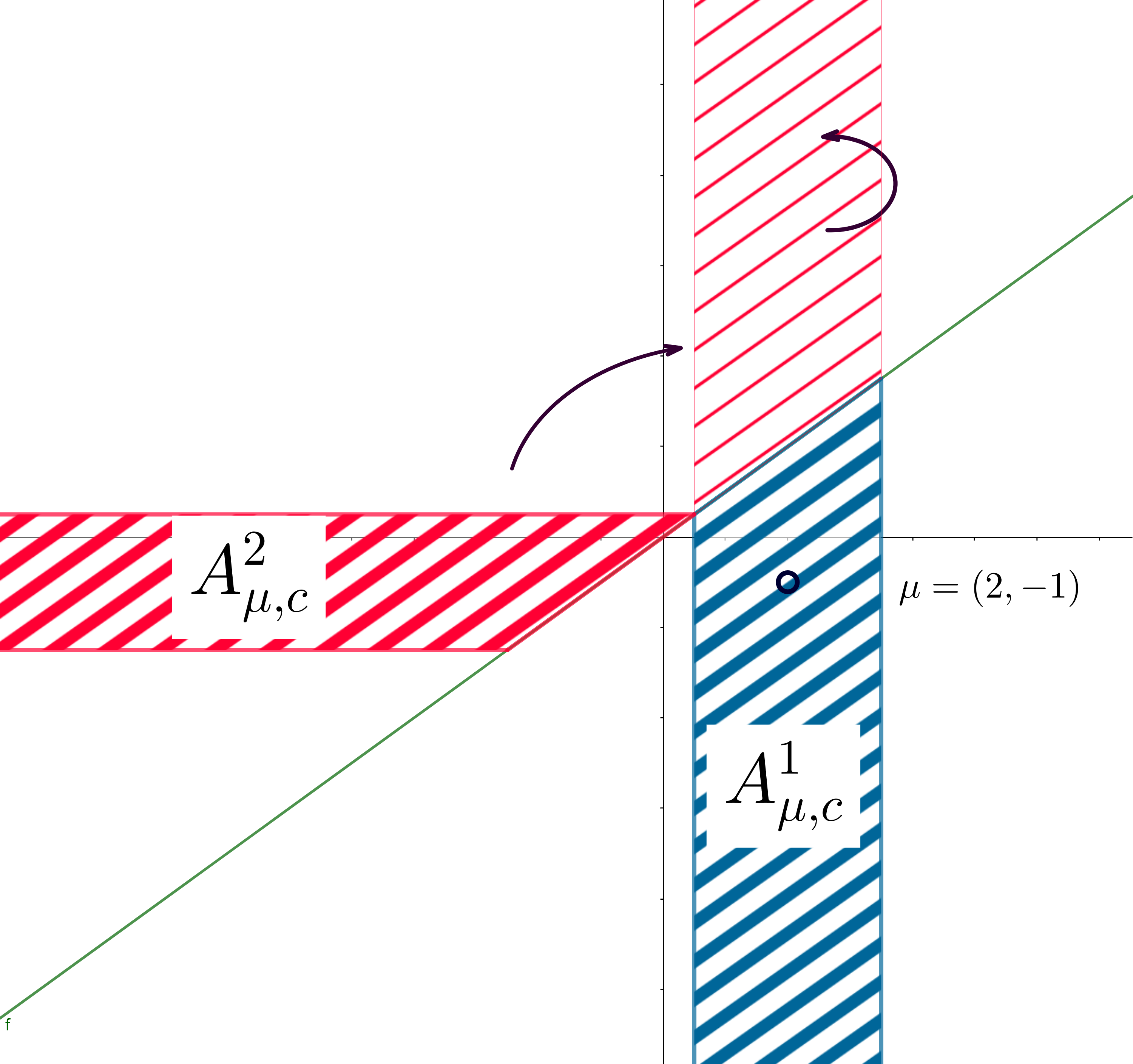
Figure 1: The semi-infinite trapezoids that comprise the acceptance region $A_{\mu,c}$. The blue hashed region is $A_{\mu_{1},c}^{1}$ and the dark red hashed region is $A_{\mu_{2},c}^{2}$. Exchangeability and symmetry of $\{Y_{i}-\theta_{i}\}$ imply that the probability of the lighter red region is equal to that of the dark red region if $\theta=\mu$, for every $\mu\in\Re^{2}$.

The proposition shows that $A_{\mu,c_{\alpha/2}}$ is the acceptance region for a level $\alpha$ test of the hypothesis $\theta=\mu$. As mentioned above, inverting tests of this form yields the confidence interval

$$\mathcal{I}(y)\equiv[y_{(1)}-c_{\alpha/2},y_{(1)}+c_{\alpha/2}].$$ (14)

This is the standard two-sided univariate symmetric confidence interval, based on the larger of the two observations. The standard two-sided univariate confidence interval has the right coverage probability despite the selection and the dependence.

3.2 Larger absolute value of two normal estimators

This section addresses constructing a confidence interval for the component selected by the rule $S(y)=\arg\max_{i}|y_{i}|$, where $Y\sim N(\theta,I)$ with $\theta\in\Re^{2}$. (Since the two estimators have normal distributions, the probability of a tie is zero.) As above, we find the intervals by inverting a family of hypothesis tests. The acceptance regions for the tests are again a union of two pieces, but they are more complicated than those in section 3.1.

3.2.1 Acceptance regions

The acceptance region $B_{\mu,c}$ for testing the hypothesis $\theta=\mu$ is

$$B_{\mu,c_{\mu}}\equiv B_{\mu_{1},c_{\mu}}^{1}\cup B_{\mu_{2},c_{\mu}}^{2},$$ (15)

where

$$B_{\mu_{i},c_{\mu}}^{i}\equiv\left\{y\in\Re^{2}:|\mu_{i}-y_{i}|\leq c_{\mu}\mbox{ and }|y_{i}|>|y_{j}|,j\neq i\right\},$$ (16)

and $c_{\mu}$ is chosen so that the test has level $\alpha$. Figure 2 plots acceptance regions for six values of $\mu$.

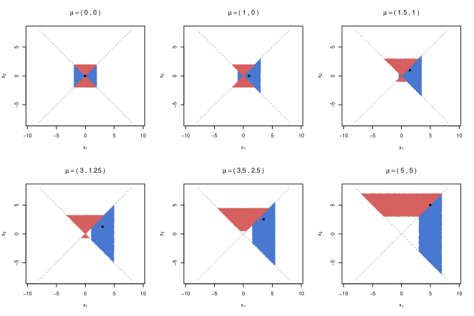
Figure 2: $B_{\mu,c}$ for various values of $\mu$ (the black dot in the figures). The blue area is $B_{\mu_{1},c}^{1}$ and the cayenne area is $B_{\mu_{2},c}^{2}$.

3.2.2 Finding $c_{\mu}$

The constant $c_{\mu}$ is the smallest $c$ for which $\mathbb{P}_{\mu}\left\{Y\in B_{\mu,c}\right\}\geq 1-\alpha$. At $\mu=0$, $B_{0,c_{0}}$ is a square; so, $c_{0}$ is Šidák’s constant $c_{\textnormal{\v{S}id}}$. We will bound $c_{\mu}$ for $\mu\neq 0$.

Proposition 2.

Let $a\equiv\max(|\mu_{1}|,|\mu_{2}|)$. For for all $c>0$,

$$\mathbb{P}_{\mu}\left\{Y\in B_{\mu,c}\right\}\geq\mathbb{P}_{(a,0)}\left\{Y\in B_{(a,0),c}\right\}.$$ (17)

The proof is in appendix A. Define

$$c_{\mu}^{+}\equiv c_{(|\mu_{1}|\vee|\mu_{2}|,0)}=c_{(0,|\mu_{1}|\vee|\mu_{2}|)}.$$ (18)

By Proposition 2, $c_{\mu}^{+}\geq c_{\mu}$. Explicit calculation gives

$$\mathbb{P}_{\mu}\left\{Y\in B_{\mu,c_{\mu}^{+}}\right\}=\sum_{i\in\{1,2\}}\intop_{-c}^{c}\phi(t)\left[\Phi(t+\mu_{i}-\mu_{i^{\prime}})-\Phi(-t-\mu_{i}-\mu_{i^{\prime}})\right](-1)^{1_{t+\mu_{i}<0}}dt,$$ (19)

where $i^{\prime}=3-i$. The value of $c_{\mu}^{+}$ is the smallest $c$ for which (19) is at least $1-\alpha$.

Hence, tests using $c_{\mu}^{+}$ instead of $c_{\mu}$ have level no larger than $\alpha$, and inverting them will give confidence intervals with coverage probability at least $1-\alpha$. Figure 3 plots $c_{\mu}^{+}$ as a function of $\max(|\mu_{1}|,|\mu_{2}|)$.

Figure 3: The upper bound $c_{\mu}^{+}$ as a function of $\max(|\mu_{1}|,|\mu_{2}|)$.

As $\max(|\mu_{1}|,|\mu_{2}|)$ grows, $c_{\mu}^{+}$ decreases monotonically; $c_{(3,0)}\approx z_{1-\frac{\alpha}{2}}$, the half-width of a standard univariate normal confidence interval.

3.2.3 The confidence interval

For $|y_{1}|>|y_{2}|$, the confidence interval for $\theta_{1}$ is:

$$\mathcal{I}_{1}(y)=[\mu_{-},\mu_{+}],$$

where

$$\mu_{-}=\inf\{a\in\Re:a+c_{(a,0)}\geq y_{1}\}$$

$$\mu_{+}=\sup\{a\in\Re:a-c_{(a,0)}\leq y_{1}\}.$$

Since $|c_{(\mu_{1},0)}|\leq c_{(0,0)}$, both endpoints are between $y_{1}-c_{(0,0)}$ and $y_{1}+c_{(0,0)}$: the interval is shorter than Šidák’s simultaneous interval. For $\alpha=0.05$, the interval is widest when $y\approx(\pm 2.23,0)$; there, the acceptance region for $\mu=0$ just includes $y$. The maximum width is about $93.6\%$ of the width of the Šidák intervals. As $|y_{1}|\rightarrow\infty$, the length converges to that of the standard unadjusted confidence interval, about 88% of the length of the Šidák interval.

Unlike the SoS interval for the larger of two, this SoS interval for the larger absolute value of two does not automatically work when $\{Y_{i}\}$ are dependent, because $\mathbb{P}_{\mu}\{Y\in B_{\mu,c}\}$ can be lower than it is when they are independent (see Hechtlinger [2014]). Acceptance regions for parameters with dependent estimators could be calibrated by brute force computation, then inverted computationally to construct confidence intervals.

4 Largest $k$ of $m$

Rather than construct a confidence interval for the single parameter estimated to be the larger of $2$, as in section 3.1, in this section we construct SoS-controlling confidence intervals corresponding for the $k$ parameters estimated to be the largest of $m$ parameters.

Consider $m$ independent random variables $Y=(Y_{1},\ldots,Y_{m})$. Let $F_{\theta_{i}}^{i}$ be the CDF of $Y_{i}$, where $F_{\zeta}^{i}(y)=F_{0}^{i}(y-\zeta)$. Let $Y_{{(1)}}\geq Y_{{(2)}}\geq\cdots\geq Y_{{(m)}}$ be the order statistics of $\{Y_{1},\ldots,Y_{m}\}$. Let $y=\left(y_{1},\ldots,y_{m}\right)\in\Re^{m}$ and let $y_{{(1)}}\geq y_{{(2)}}\geq\cdots\geq y_{{(m)}}$ be the observed order statistics.

Consider the selection rule $S_{k}(\cdot)$ that keeps the components corresponding to the largest $k$ components of $Y$, with ties broken lexicographically, and let $S_{k}^{c}(y)\equiv\{1,\ldots,m\}\setminus S_{k}(y)$. Let $|s|$ denote the cardinality of the set $s$, so $|S_{k}(y)|=k$. Let $\mathcal{S}_{k}\equiv\{s\subset\{1,\ldots,m\}:|s|=k\}$.

Since $S$ contains the $k$ components for which $Y_{i}$ is largest, one might expect the conditional distribution $Y_{i}$ given $i\in S$ to be stochastically larger than its unconditional distribution. It is, which allows us control the chance that the upper endpoint of any interval is below its parameter using a Bonferroni adjustment with multiplicity $k$ rather than $m$.

Consider the $k$ intervals

$$\mathcal{I}_{{(i)}}(y)\equiv[y_{{(i)}}-\text{\@text@baccent{$c$}}_{i},y_{{(i)}}+\bar{c}_{i}],\;\;1\leq i\leq k,$$ (20)

where $\text{\@text@baccent{$c$}}_{i}\equiv(F_{0}^{i})^{-1}(1-\text{\@text@baccent{$\lambda$}})$ and $\bar{c}_{i}\equiv-(F_{0}^{i})^{-1}(\bar{\lambda})$, $i=1,\ldots,m$, with $\text{\@text@baccent{$\lambda$}}>0$, $\bar{\lambda}>0$, and $\text{\@text@baccent{$\lambda$}}+\bar{\lambda}<1$

Proposition 3.

$$\mathbb{P}\left\{\exists i\in\{1,\ldots,m\}:\mathcal{I}_{{(i)}}\not\ni\theta_{{(i)}}\right\}\leq m\text{\@text@baccent{$\lambda$}}+k\bar{\lambda}.$$ (21)

Corollary 4.

For all $\delta\in(0,1)$, if $\text{\@text@baccent{$\lambda$}}=\delta\alpha/m$ and $\bar{\lambda}=(1-\delta)\alpha/k$, then the intervals defined in equation 20 have $1-\alpha$ SoS coverage.

Corollary 4 defines a family of intervals that control SoS at level $\alpha$. The intervals are in general asymmetric, and the chance that the intervals miss the parameter from below is not in general equal to the chance that they miss from above. For $\delta=\frac{1}{2}$, neither the expected rate at which the upper endpoint is below its parameter nor the expected rate at which the lower endpoint is above its parameter exceeds $\alpha/2$. When $\{F_{0}^{i}\}$ are all symmetric, setting $\delta=m/(m+k)$ gives symmetric intervals corresponding to the two sided $m+k$ Bonferroni correction.

When $\{F_{0}^{i}\}$ are all equal, finding the $\delta$ that yields the shortest intervals is a 1-dimensional optimization problem. Figure 4 plots the length of the intervals for different values of $k$ and $m$ when $Y_{i}\sim N(\theta_{i},1)$. Because $S$ selects large components, the shortest intervals extend below $Y_{i}$ by more than they extend above $Y_{i}$.

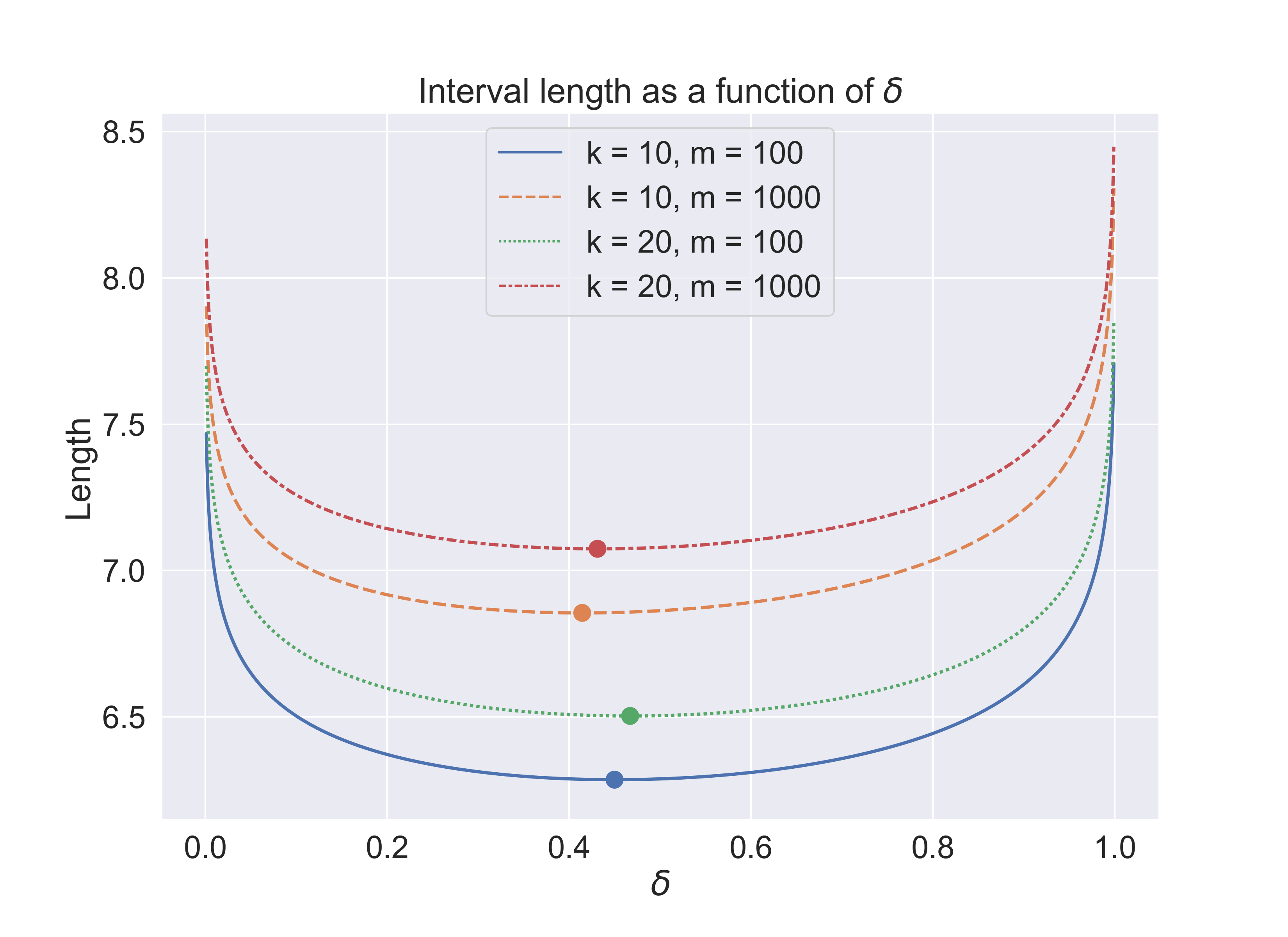
Figure 4: Lengths of the confidence intervals as a function of $k$, $m$, and $\delta$, for $\alpha=0.05$. The dots are plotted at the minimizing values of $\delta$; lengths are nearly minimal when $\delta\approx 0.45$.

Proof of Proposition 3.

Define

$$\text{\@text@baccent{$V$}}_{i}=\begin{cases}1,&y_{i}-\text{\@text@baccent{$c$}}_{i}>\theta_{i}\\ 0,&\text{otherwise}\end{cases};\;\;\bar{V}_{i}=\begin{cases}1,&y_{i}+\bar{c}_{i}<\theta_{i}\\ 0,&\text{otherwise}\end{cases}$$ (22)

and

$$\text{\@text@baccent{$V$}}_{{(i)}}=\begin{cases}1,&y_{{(i)}}-\text{\@text@baccent{$c$}}_{i}>\theta_{{(i)}}\\ 0,&\text{otherwise}\end{cases};\;\;\bar{V}_{{(i)}}=\begin{cases}1,&y_{{(i)}}+\bar{c}_{i}<\theta_{{(i)}}\\ 0,&\text{otherwise.}\end{cases}$$ (23)

Now $\mathcal{I}_{{(i)}}\not\ni\theta_{{(i)}}$ if either $Y_{{(i)}}-\text{\@text@baccent{$c$}}_{i}>\theta_{{(i)}}$ (then the lower endpoint of the interval is greater than $\theta_{{(i)}}$, and $\text{\@text@baccent{$V$}}_{{(i)}}=1$) or $Y_{{(i)}}+\bar{c}_{i}<\theta_{{(i)}}$ (then the upper endpoint of the interval is below $\theta_{{(i)}}$, and $\bar{V}_{{(i)}}=1$).

Since $\text{\@text@baccent{$V$}}_{{(i)}}=1$ and $\bar{V}_{{(i)}}=1$ are mutually exclusive, the event $\mathcal{I}_{{(i)}}\not\ni\theta_{{(i)}}$ is the event $\text{\@text@baccent{$V$}}_{{(i)}}+\bar{V}_{{(i)}}=1$. Let $\text{\@text@baccent{$V$}}\equiv\sum_{i=1}^{k}\text{\@text@baccent{$V$}}_{{(i)}}$ and $\bar{V}\equiv\sum_{i=1}^{k}\bar{V}_{{(i)}}$. The event that at least one interval does not cover its parameter is the event $\text{\@text@baccent{$V$}}+\bar{V}\geq 1$. Hence,

$$\mathbb{P}\{\exists i:\mathcal{I}_{{(i)}}\not\ni\theta_{{(i)}}\}=\mathbb{P}\left\{\text{\@text@baccent{$V$}}+\bar{V}\geq 1\right\}\leq\mathbb{P}\left\{\text{\@text@baccent{$V$}}\geq 1\right\}+\mathbb{P}\left\{\bar{V}\geq 1\right\}.$$ (24)

The first term on the right hand side is

$$\mathbb{P}\left\{\text{\@text@baccent{$V$}}\geq 1\right\} \leq\sum_{i=1}^{k}\mathbb{P}\left\{\text{\@text@baccent{$V$}}_{{(i)}}=1\right\}\leq\sum_{i=1}^{m}\mathbb{P}\left\{\text{\@text@baccent{$V$}}_{{(i)}}=1\right\}$$

$$=\sum_{i=1}^{m}\mathbb{P}\left\{\text{\@text@baccent{$V$}}_{i}=1\right\}=\sum_{i=1}^{m}\mathbb{P}\left\{Y_{i}-\theta_{i}>\text{\@text@baccent{$c$}}_{i}\right\}$$

$$=m\text{\@text@baccent{$\lambda$}}.$$ (25)

The second term on the right of (24) is

$$\mathbb{P}\left\{\bar{V}\geq 1\right\} =\mathbb{P}\left\{\exists i\in S(Y):\bar{V}_{i}=1\right\}$$

$$=\sum_{s\in\mathcal{S}_{k}}\mathbb{P}\left\{S(Y)=s\cap\exists i\in s:\bar{V}_{i}=1\right\}$$

$$\leq\sum_{s\in\mathcal{S}_{k}}\sum_{i\in s}\mathbb{P}\left\{S(Y)=s\cap\bar{V}_{i}=1\right\}$$

$$=\sum_{s\in\mathcal{S}_{k}}\sum_{i\in s}\mathbb{P}\left\{S(Y)=s\;\mid\;\bar{V}_{i}=1\right\}\mathbb{P}\{\bar{V}_{i}=1\}$$

$$=\sum_{s\in\mathcal{S}_{k}}\sum_{i\in s}\mathbb{P}\left\{S(Y)=s\;\mid\;\bar{V}_{i}=1\right\}\bar{\lambda}$$

$$=\bar{\lambda}\sum_{s\in\mathcal{S}_{k}}\sum_{i\in s}\mathbb{P}\left\{\min_{j\in s}Y_{j}\geq\max_{k\in s^{c}}Y_{k}\;\mid\;Y_{i}<\theta_{i}-\bar{c}_{i}\right\}$$

Let $\tilde{F}_{\theta_{i}}(y)\equiv\mathbb{P}\{Y_{i}\leq y\mid Y_{i}<\theta_{i}-\bar{c}_{i}\}$. Then for all $y\in\Re$,

$$\tilde{F}_{\theta_{i}}(y) =\frac{\mathbb{P}\{Y_{i}\leq y\cap Y_{i}<\theta_{i}-\bar{c}_{i}\}}{\mathbb{P}\{Y_{i}<\theta_{i}-\bar{c}_{i}\}}$$

$$=\begin{cases}F_{\theta_{i}}(y)/F_{\theta_{i}}(\theta_{i}-\bar{c}_{i}),&y<\theta_{i}-\bar{c}_{i}\\ 1,&y\geq\theta_{i}-\bar{c}_{i}\end{cases}$$

$$\geq F_{\theta_{i}}(y).$$

By Theorem 4.12.3 of Grimmett and Stirzaker [2001], there exists a random variable $\tilde{Y}_{i}$ independent of $\{Y_{j}\}_{j\neq i}$ such that $\tilde{Y}_{i}\sim\tilde{F}_{\theta_{i}}$ and

$$\mathbb{P}\{\tilde{Y}_{i}(\omega)\leq Y_{i}(\omega)\}~{}=~{}1.$$

Hence,

$$\mathbb{P}\left\{\min_{j\in s}Y_{j}\geq\max_{k\in s^{c}}Y_{k}\;\mid\;Y_{i}<\theta_{i}-\bar{c}_{i}\right\} =\mathbb{P}\left\{\min(Y_{i},\min_{j\in s\setminus i}Y_{j})\geq\max_{k\in s^{c}}Y_{k}\;\mid\;Y_{i}<\theta_{i}-\bar{c}_{i}\right\}$$

$$=\mathbb{P}\left\{\min(\tilde{Y}_{i},\min_{j\in s\setminus i}Y_{j})\geq\max_{k\in s^{c}}Y_{k}\right\}$$

$$\leq\mathbb{P}\left\{\min(Y_{i},\min_{j\in s\setminus i}Y_{j})\geq\max_{k\in s^{c}}Y_{k}\right\}$$

$$=\mathbb{P}\left\{\min_{j\in s}Y_{j}\geq\max_{k\in s^{c}}Y_{k}\right\}$$

$$=\mathbb{P}\{S(Y)=s\},$$

where the first step uses the independence of $\{Y_{j}\}$. Thus

$$\mathbb{P}\left\{\bar{V}\geq 1\right\} \leq\bar{\lambda}\sum_{s\in\mathcal{S}_{k}}\sum_{i\in s}\mathbb{P}\left\{S(Y)=s\right\}$$

$$=\bar{\lambda}\sum_{s\in\mathcal{S}_{k}}k\mathbb{P}\left\{S(Y)=s\right\}$$

$$=k\bar{\lambda}.$$ (26)

Combining (24), (25), and (26) yields the desired result. ∎

5 Comparisons

Bonferroni confidence intervals are of the form $[Y_{j}-c_{,}Y_{j}+c]$, with

$$c=-\sup\{c:\mathbb{P}\{Y_{i}-\theta_{i}\leq c\}\leq\alpha/(2m)\}.$$ (27)

Bonferroni confidence intervals control SoP (and consequently SoS) even when $\{Y_{i}\}$ are dependent. When $\{Y_{i}\}$ are independent, Šidák confidence intervals, which are of the same form but with

$$c=-\sup\{c:\mathbb{P}\{Y_{i}-\theta_{i}\leq c\}\leq(1-(1-\alpha)^{1/m})/2\},$$ (28)

offer a small (but optimal) improvement on Bonferroni intervals.

Fuentes et al. [2018] construct SoS intervals for this $k$ out of $m$ problem with $\{Y_{i}-\theta_{i}\}$ are IID $N(0,1)$. Their intervals, which we call FCW, are of the form $[Y_{j}-c,Y_{j}+d]$, where $c$ and $d$ are constants such that

$$\left[\Phi\left(c\right)-\Phi\left(-d\right)\right]^{k-1}\times\left[\Phi^{m-k+1}\left(c\right)-\Phi^{m-k+1}\left(-d\right)\right]\geq 1-\alpha.$$ (29)

Figure 5 compares the Bonferroni intervals, the Šidák intervals, FCW intervals (with $c=d$ and with $c$ and $d$ chosen to make the intervals as short as possible), and the SoS intervals (with $\delta$ chosen to make the intervals symmetric or as short as possible).

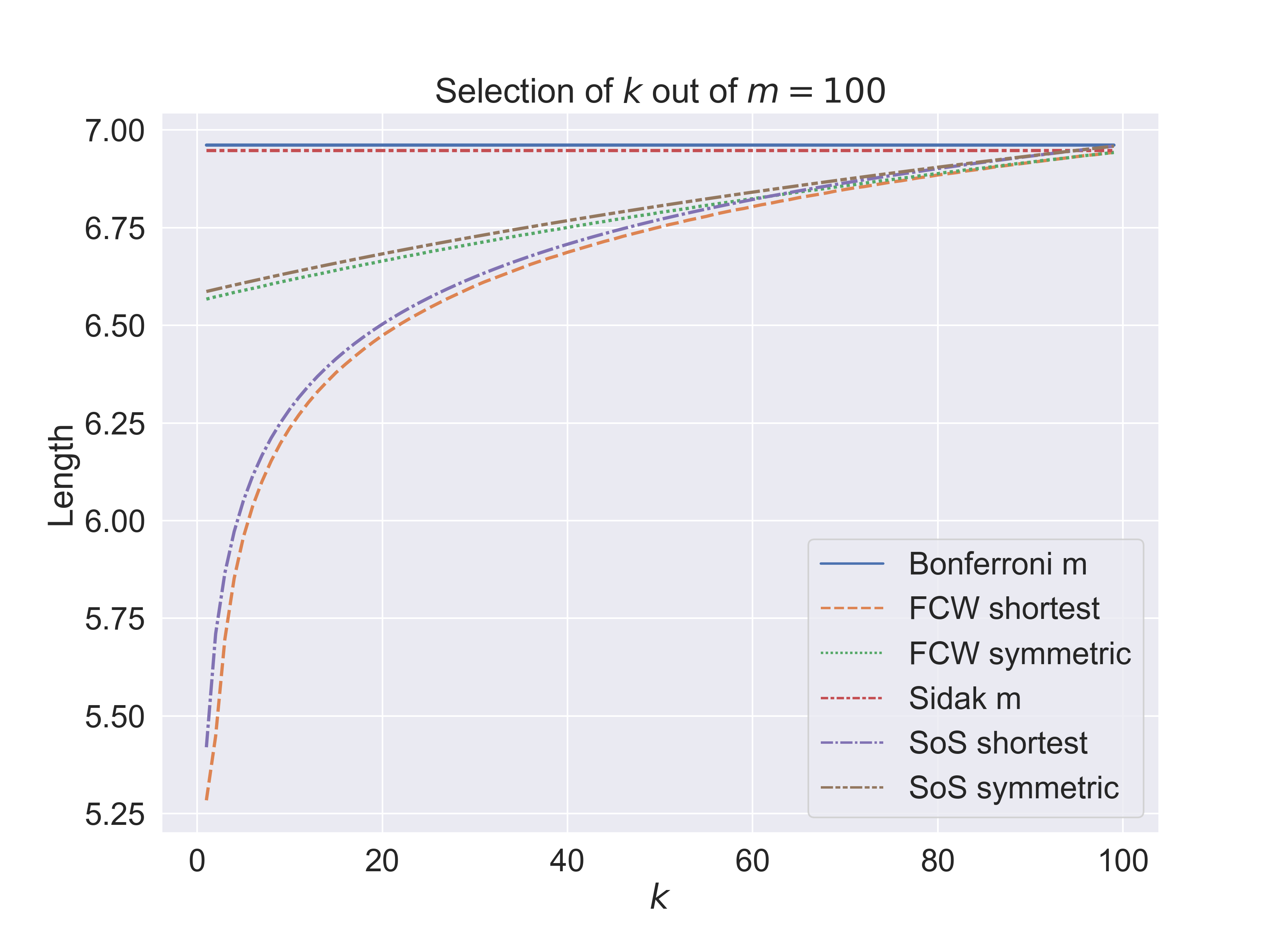
Figure 5: Lengths of confidence intervals with simultaneous coverage of the $k$ of $m=100$ normal means estimated to be largest, for $\alpha=0.05$.

Because SoS intervals make inferences about only $k<m$ parameters, one would expect them to be narrower than SoP intervals—but not as narrow as intervals for a pre-specified set $k$ parameters: there should be some penalty for the selection. (The case $m=2$, $k=1$ is a remarkable exception.) Letting the intervals be asymmetric can reduce their length further. Suppose all the parameters are equal. Because $S$ selects the largest $k$, $S$ will preferentially select components for which $Y_{i}>\theta_{i}$. Using intervals that extend below $Y_{i}$ more than they extend above $Y_{i}$ allows the intervals to be shorter. Figure 5 shows that the advantage of allowing asymmetry is substantial when $k\ll m$. The SoS intervals are slightly wider than the FCW intervals, but the FCW intervals require $\{Y_{i}-\theta_{i}\}$ to have normal distributions, while the SoS intervals do not.

Weinstein et al. [2013], Fithian et al. [2014] and Reid et al. [2017] develop CoS intervals for the largest $k$ of $m$. Controlling CoS controls FCR. These intervals also control SoS if each interval is constructed at level $1-\alpha/|S|$, rather than $1-\alpha$.

CoS intervals use conditional distributions, which depend on the conditioning event and the underlying parameters of the model. As a result, CoS intervals are sometimes useful and sometimes not. For instance, CoS intervals for the largest of $m$ or largest absolute value of $m$ can be too wide to be useful when the largest and second-largest estimators are close [Fithian et al., 2015]. Table 1 shows the uniformly most powerful unbiased (UMPU) CoS intervals from example 4 in Fithian et al. [2014] when $\left(Y_{1},Y_{2}\right)$ is bivariate uncorrelated normal centered at $\left(\theta_{1},\theta_{2}\right)$, for the observed value $\left(y_{1},y_{2}\right)=\left(2.9,2.5\right)$ and the greater $S\left(Y\right)=\left\{\left(1\right)\right\}$ is selected. In section 3, we showed that the unadjusted univariate interval has the right coverage. The UMPU saturated CoS intervals use $\mathbb{P}_{\theta_{1}}\left(Y_{1}|Y_{1}>2.5\right)$. For $\theta_{1}\ll 2.5$, the conditional distribution is a renormalized tail of the distribution, which yields long intervals. The UMPU selected CoS intervals use $\mathbb{P}_{\left(\theta_{1},\theta_{2}\right)}\left(Y_{1}\mid Y_{1}>Y_{2}\right)$. Then, the underlying distribution is a function of both $\theta_{1}$ and $\theta_{2}$. Setting $\theta_{2}=0$ produces “nicer” intervals than $\theta_{2}=2.5$ because the selection event has less effect on the conditional distribution. But while setting the coefficient of an unselected variable to zero in a model might make sense, for location parameters, setting $\theta_{2}=0$ when it is estimated to be $2.5$ does not. This shows the importance of the unselected parameters to the coverage of selected parameters. Furthermore, if a coverage were needed for all $\theta_{2}$, the interval would have an infinite lower tail, since for all $\theta_{1}\ll 2.5$ there exist $\theta_{2}\gg 2.5$ such that $\mathbb{P}_{\left(\theta_{1},\theta_{2}\right)}\left(Y_{1}|Y_{1}>Y_{2}\right)$ is centered at $2.9$.

Because the lengths of CoS intervals depend on the observed value of $Y$ (not only on $k$ and $m$), we do not include CoS intervals in our figures or numerical comparisons.

	$\theta_{1}\in\left(\text{Lower},\text{Upper}\right)$	Length
Marginal / SoS	$\left(0.940,4.859\right)$	$3.919$
$\mathbb{P}_{\theta_{1}}\left(Y_{1}|Y_{1}>2.5\right)$ - UMPU saturated	$\left(-9.090,4.594\right)$	$13.684$
$\mathbb{P}_{\left(\theta_{1},0\right)}\left(Y_{1}|Y_{1}>Y_{2}\right)$ - UMPU selected $\left(\theta_{2}=0\right)$	$\left(0.772,4.855\right)$	$4.082$
$\mathbb{P}_{\left(\theta_{1},2.5\right)}\left(Y_{1}|Y_{1}>Y_{2}\right)$ - UMPU selected $\left(\theta_{2}=2.5\right)$	$\left(-0.224,4.558\right)$	$4.782$
$\mathbb{P}_{\left(\theta_{1},\theta_{2}\right)}\left(Y_{1}|Y_{1}>Y_{2}\right)$ - UMPU selected $\left(\forall\theta_{2}\in\Re\right)$	$\left(-\infty,4.859\right)$	$\infty$

Table 1: Intervals for $\alpha=0.05$ for the bivariate normal after selecting the greater of the two estimators when $\left(y_{1},y_{2}\right)=\left(2.9,2.5\right)$. The depicted UMPU saturated and selected CoS intervals are from Fithian et al. [2014].

6 Discussion

Katsevich and Ramdas [2018] address “simultaneous selective inference” in testing. They consider making selective inference statements on many selection rules $\left\{S_{i}\left(Y\right)\right\}$, guaranteeing this statements hold simultaneously with high probability. By restricting the possible selections to those determined by a particular algorithm, for instance, those obtained by varying the level at which FDR is controlled, their method can improve on full simultaneity.

We have shown that knowing the selection rule $S$ can improve inferences, for instance by allowing one to control SoS or CoS without necessarily controlling SoP. More information is better. Lee et al. [2016] and Tibshirani et al. [2016] constructed confidence interval for parameters selected by the Lasso and by forward stepwise selection, respectively.

For SoP and FCR, it is not necessary to know $S$, but if $S$ is known, improvements are possible. Berk et al. [2013] addressed the problem of inference when the model is selected because a pre-specified explanatory variable had the highest statistical significance, which restricts the family over which simultaneous coverage is required. The restriction transforms the problem into that of making a confidence interval for the coefficient whose estimate is most significantly nonzero among many correlated estimates. This amounts to selecting on the basis of the largest 1 of $m$ correlated statistics, which can be solved computationally for problems of modest dimension. If the design matrix is orthogonal, their confidence interval amounts to the Bonferroni interval adjusted for $m$ parameters—the dimension of the relevant family. Weinstein et al. [2013] constructed CoS intervals tailored to avoid containing zero, at the expense of being somewhat longer where it does not matter and Weinstein and Yekutieli [2014] designed FCR intervals that try to avoid covering 0. Barber and Candès [2015] took advantage of the fact that their knockoff method used forward stepwise search (their method does not yet offer confidence intervals).

To see that FCR intervals can also take advantage of knowledge of $S$, consider the rule $S$ that selects the $k$ parameters estimated to be the largest of $m$. This rule always selects $k$ parameters. The proof of proposition 3 bounds the probability of making one or more errors via the expected number of upper endpoints that are smaller than their corresponding parameter plus the expected number of lower endpoints that are larger than their corresponding parameters. These expectations are bounded by a multiple of $\alpha$. FCR control requires the expected number of non-covering intervals, divided by $k$, to be at most $\alpha$. Therefore, if $S$ selects the $k$ largest of $m$, FCR intervals can have lower endpoints based on the $1-(\alpha/2)\cdot(k/m)$ quantile (which works for any simple selection rule [Benjamini and Yekutieli, 2005]), and upper endpoints based on the $\alpha/2$ quantile instead of the $(\alpha/2)\cdot(k/m)$ quantile.

In conclusion, specification of a selection rule allows us to explore the inference ground between simultaneous and false confidence statement rate controlling confidence intervals, by defining the in-between goal of simultaneous coverage one the selected. We explored the implications of this error-rate by studying the largest k-out-of-m rule. This resulted in new confidence intervals. In their simplest version, the lower endpoints are Bonferroni adjusted for m, while the upper endpoints are Bonferroni adjusted only for k, offering uniform improvement over regular Bonferroni. Furthermore, the utilization of such a selection rule allows improvement over the general FCR intervals.

It seems clear that the confidence intervals retain their coverage for positive-regression-dependent estimators, because the conditional distribution of the variables selected is stochastically greater than the same variables without selection, but we do not have a formal proof. Appendix B gives numerical evidence that this is indeed the case. The intervals may also be valid when $k$ is random, for instance when selection depends on crossing a fixed threshold or some other testing procedure.

We think the results for the $k$ largest in absolute value of $m$ extend to $m>2$ and $k>1$, but again, we offer no formal proof. We have decided to publish our current results without those generalizations with the hope that they will spark interest engage others in pursuing this approach.

Appendix A Proof of Proposition 2

Since $Y_{i}-\theta_{i}$ are IID standard normals, they are rotationally invariant and symmetric. Of course, $\mathbb{P}_{\mu}\{A\}=\mathbb{P}_{0}\{A-\mu\}$. These three properties let us find or bound $\mathbb{P}\{B_{\mu,c}\}$.

Assume without loss of generality that $mu_{1}\geq mu_{2}\geq 0$. The acceptance regions $B_{\mu,c}$ have three forms, depending on whether (1) $\mu_{1}\geq\mu_{2}\geq c$, (2) $\mu_{1}\geq c\geq\mu_{2}$, or (3) $c\geq\mu_{1}\geq\mu_{2}$.

Case (1) $\mu_{1}\geq\mu_{2}\geq c$. Because $\mu_{1}\geq c$, $B_{(\mu_{1},0),c}^{1}$ is a trapezoid and $B_{(\mu_{1},0),c}^{2}$ consists of two congruent triangles. Rotating the triangles and reflecting them about $x=\mu_{1}$ yields the hexagon in Figure 6. Because $\mu_{2}\geq c$, $B_{(\mu_{1},\mu_{2}),c}$ consists of two trapezoids. Clockwise rotation and reflection of the trapezoid $B_{(\mu_{1},\mu_{2}),c}^{2}$ yields a parallelogram. See Figure 7. The transformation $\varphi(x,y)=(x,y-\mu_{2})$ translates $(\mu_{1},\mu_{2})$ to $(\mu_{1},0)$, allowing us to compare their acceptance regions. See Figure 8.

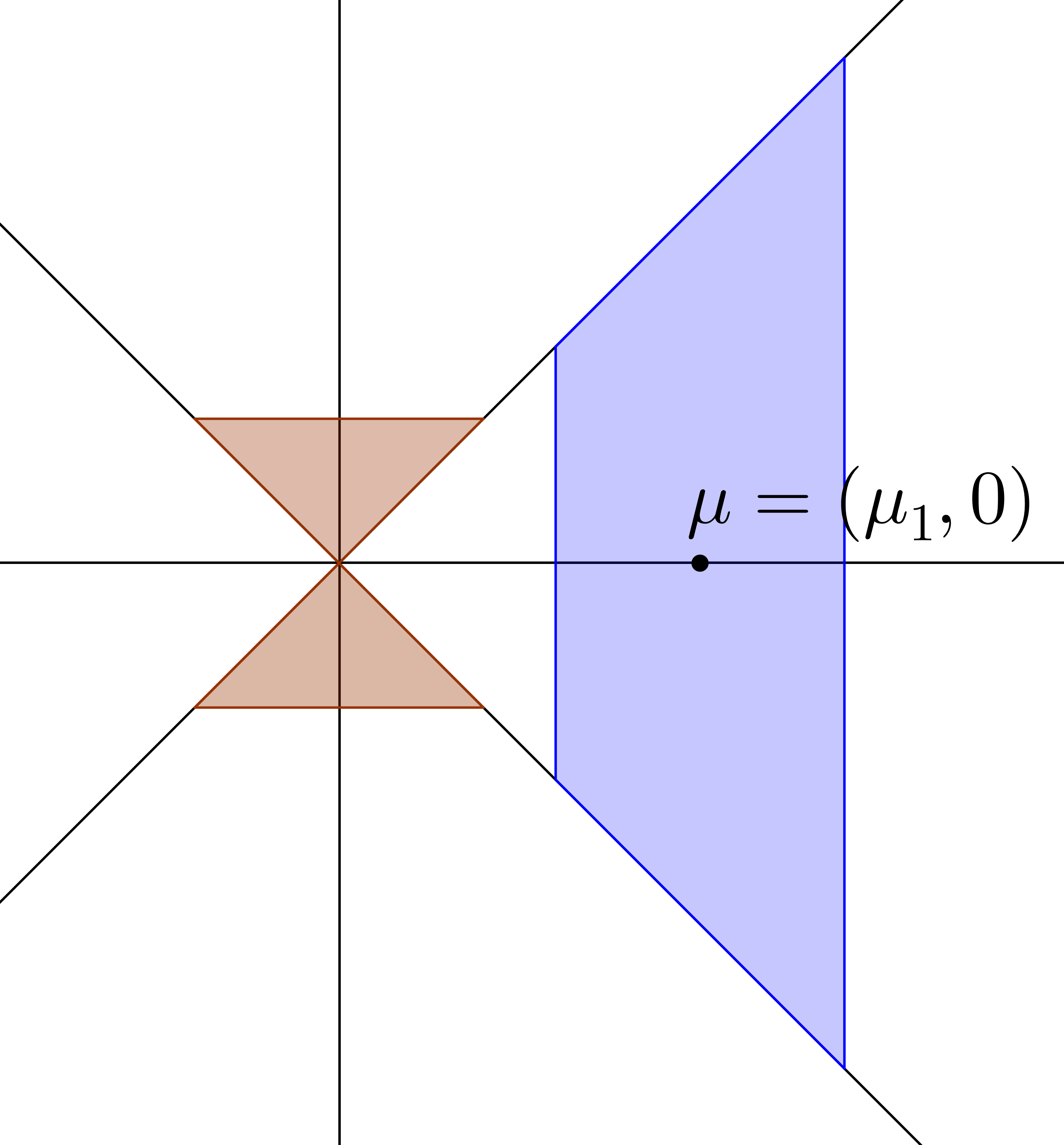
(a)

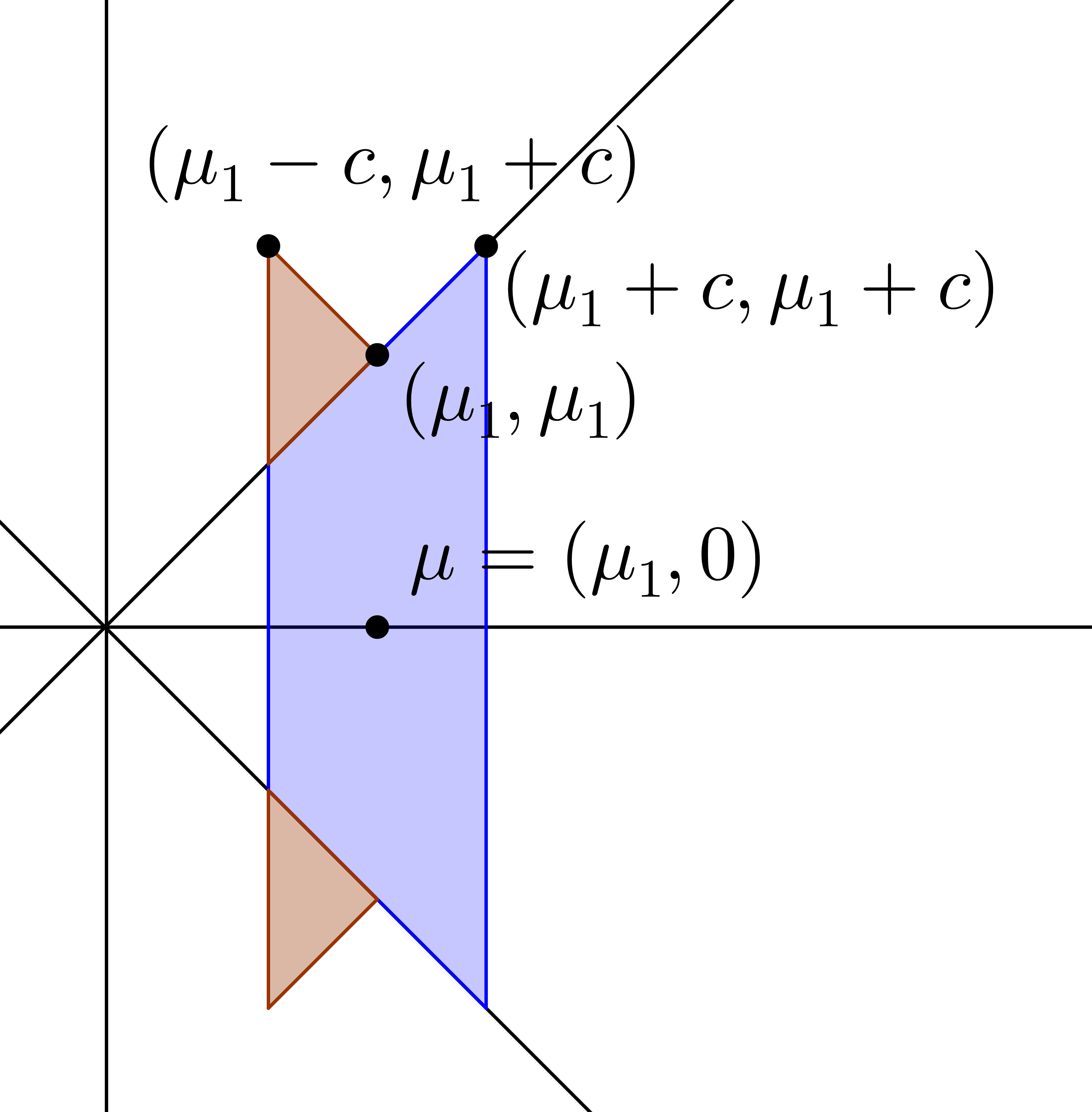
(b)

Figure 6: (a): $B_{(\mu_{1},0),c}$. (b): $B_{(\mu_{1},0),c}$ after a $\mathbb{P}_{\mu}$-preserving transformation.

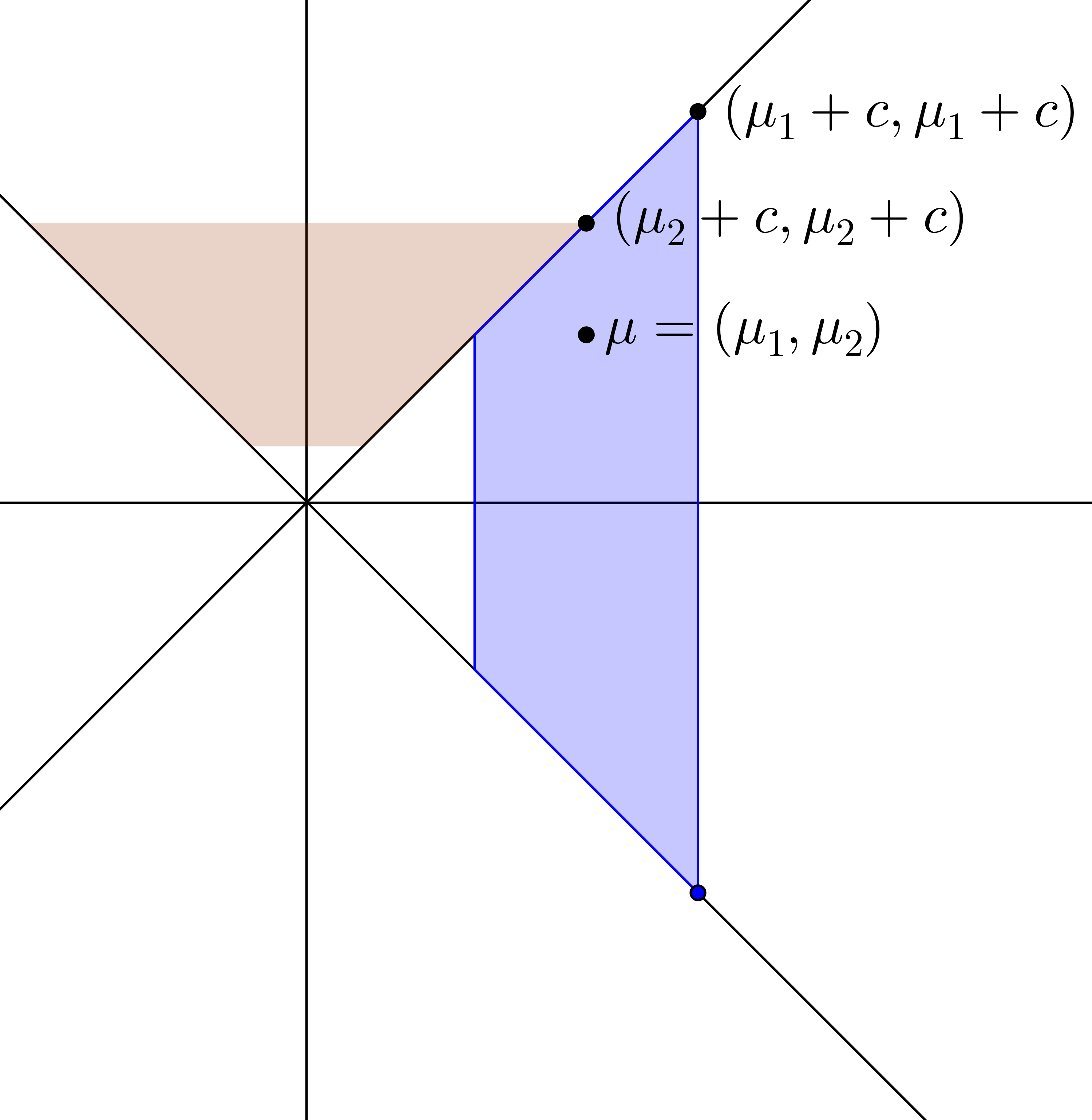
(a)

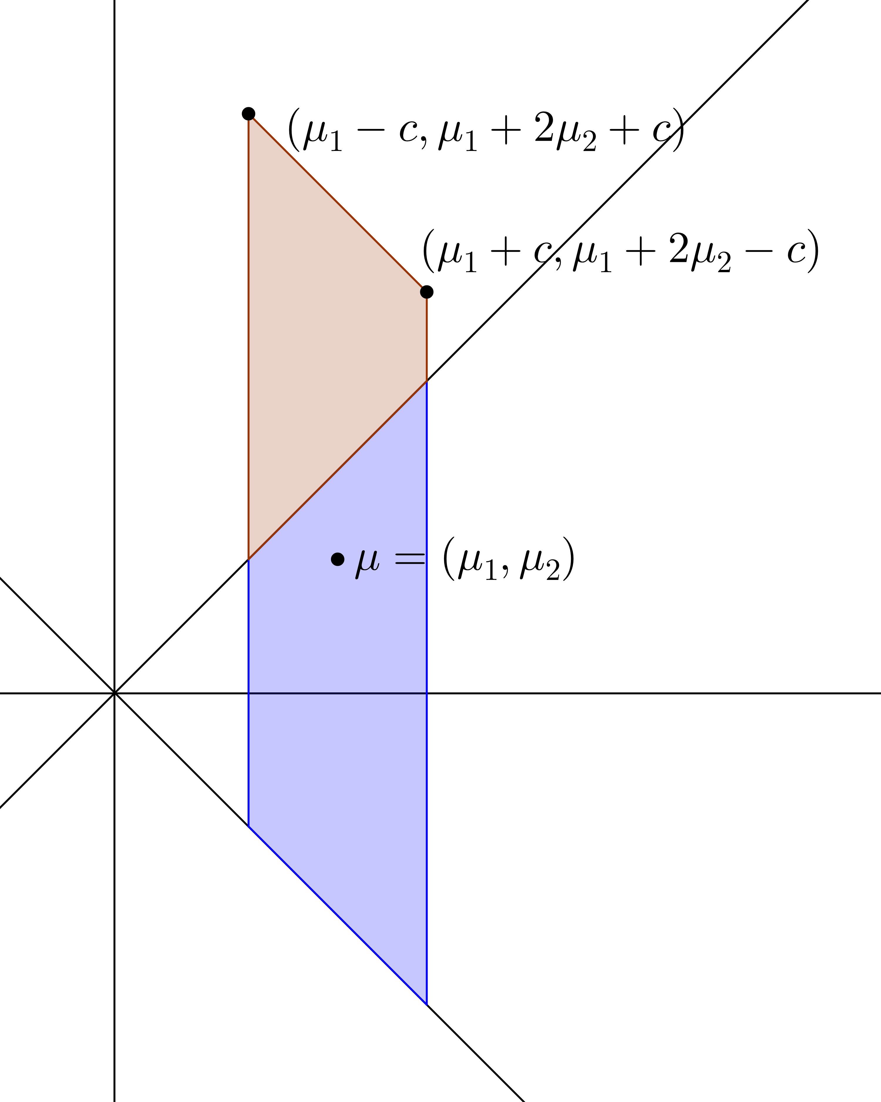
(b)

Figure 7: (a): $B_{(\mu_{1},\mu_{2}),c}$ for $\mu_{1}>\mu_{2}>c$. (b): $B_{(\mu_{1},\mu_{2}),c}$ after a $\mathbb{P}_{\mu}$-preserving transformation.

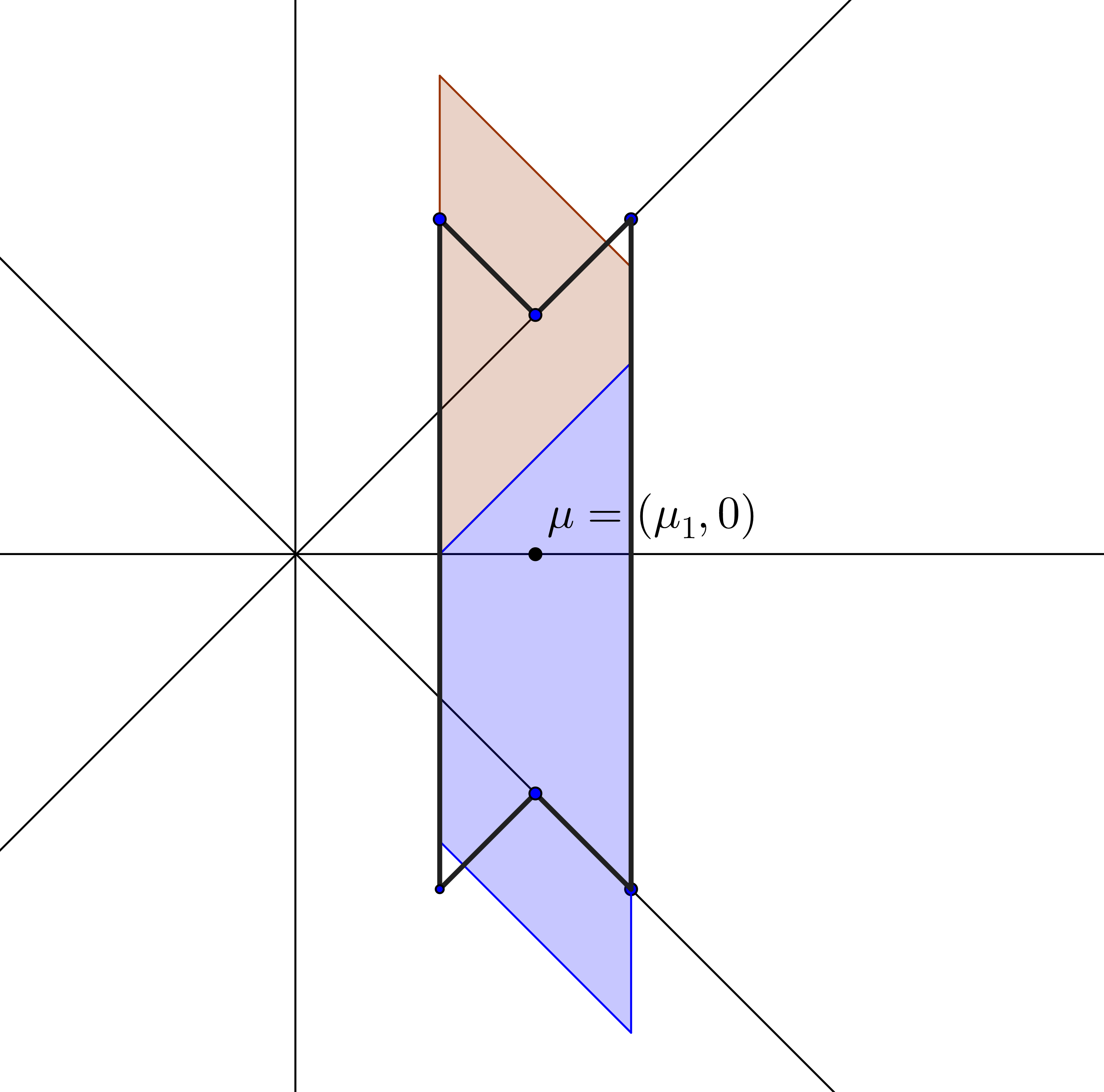
(a)

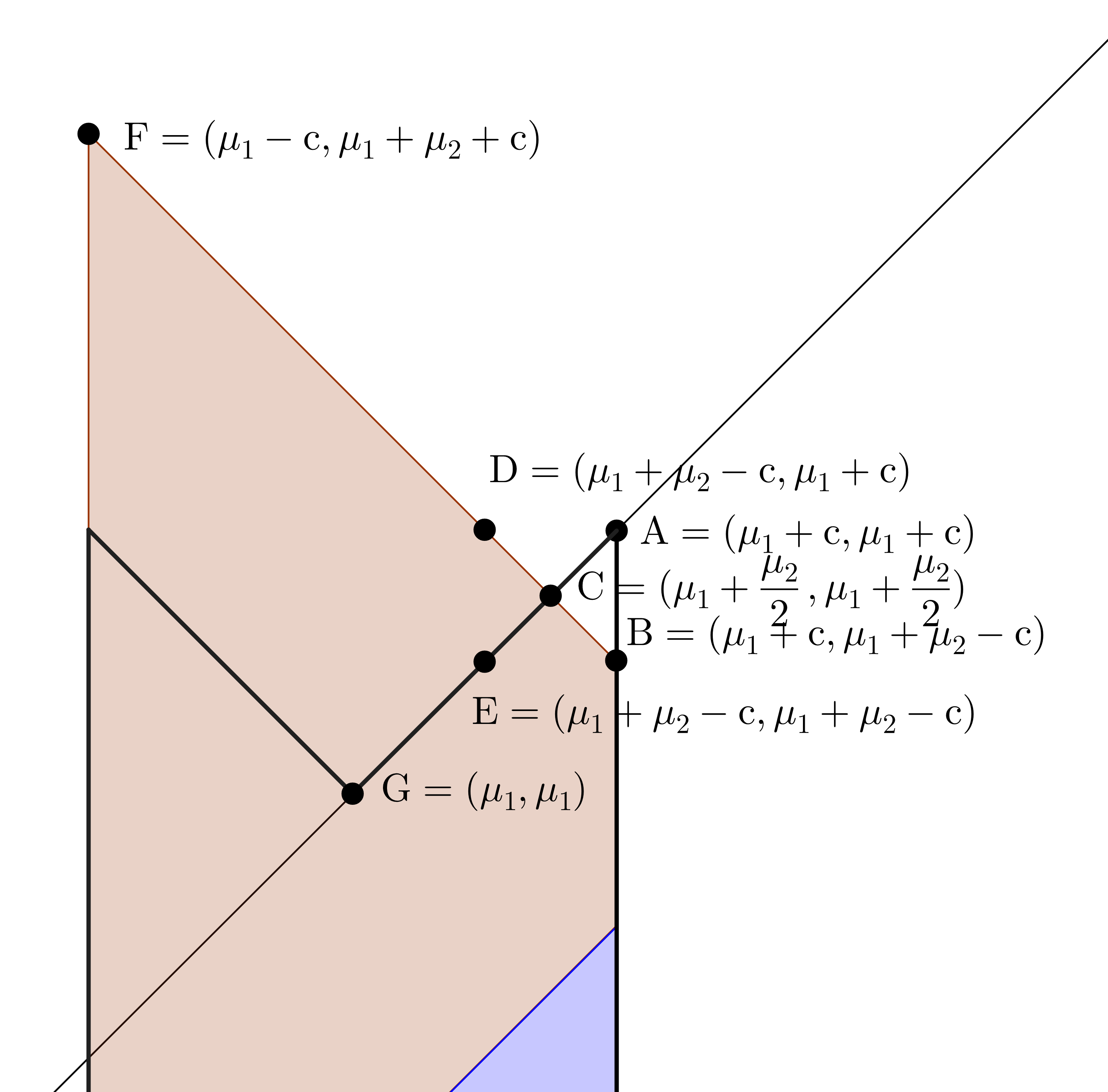
(b)

Figure 8: (a): $B_{(\mu_{1},\mu_{2}),c}$ and $B_{(\mu_{1},0),c}$ superposed after $\mathbb{P}_{\mu}$-preserving transformations when $\mu_{1}\geq\mu_{2}\geq c$. The black hexagon is $B_{(\mu_{1},0),c}$ and the shaded parallelogram is $B_{(\mu_{1},\mu_{2}),c}$ after re-centered at $(\mu_{1},0)$. (b): Detail of the top of panel (a). The bottom half of the trapezoid is the top half rotated by $\pi$, which does change its probability.

The line $\overline{FB}$ in Figure 8 (b) is $y=-x+2\mu_{1}+\mu_{2}$. It intersects $y=x$ at the point $C=\left(\mu_{1}+\mu_{2}/2,\mu_{1}+\mu_{2}/2\right)$. If $\mu_{2}/2\geq c$, then $B_{(\mu_{1},0),c}\subseteq B_{(\mu_{1},\mu_{2}),c}$. Otherwise, $D=(\mu_{1}+\mu_{2}-c,\mu_{1}+c)$ is above the point $E=(\mu_{1}+\mu_{2}-c,\mu_{1}+\mu_{2}-c)$, and to the right of $G=(\mu_{1},\mu_{1})$. Thus the triangles $\triangle CDE$ and $\triangle ABC$ are congruent. Since the reflection of $\triangle CDE$ about the horizontal line $x=\mu_{1}+\mu_{2}/2$ is $\triangle ABC$, $\mathbb{P}\{\triangle CDE\}\geq\mathbb{P}\{\triangle ABC\}$, and so $\mathbb{P}_{(\mu_{1},\mu_{2})}\{A_{(\mu_{1},\mu_{2}),c}\}\geq\mathbb{P}_{(\mu_{1},0)}\{A{}_{(\mu_{1},0),c}\}$.

Case (2) $\mu_{1}\geq c\geq\mu_{2}$. The region $B_{(\mu_{1},0),c}$ is as in case (1), but for $\mu_{2}>0$, $B_{(\mu_{1},\mu_{2}),c}^{1}$ is a trapezoid and $B_{(\mu_{1},\mu_{2}),c}^{2}$ consists of two triangles that meet at 0. Rotating the upper triangle $\pi/2$ clockwise, and the lower triangle $\frac{\pi}{2}$ counter clockwise, then reflecting both across $x=\mu_{1}$ and centering yields Figure 9. As in case (1), rotating the quadrilateral $DEFG$ about the line $x=\mu_{1}+\mu_{2}/2$, and noticing that once again the top half is congruent to the bottom half (rotated by $\pi$) establishes the conclusion.

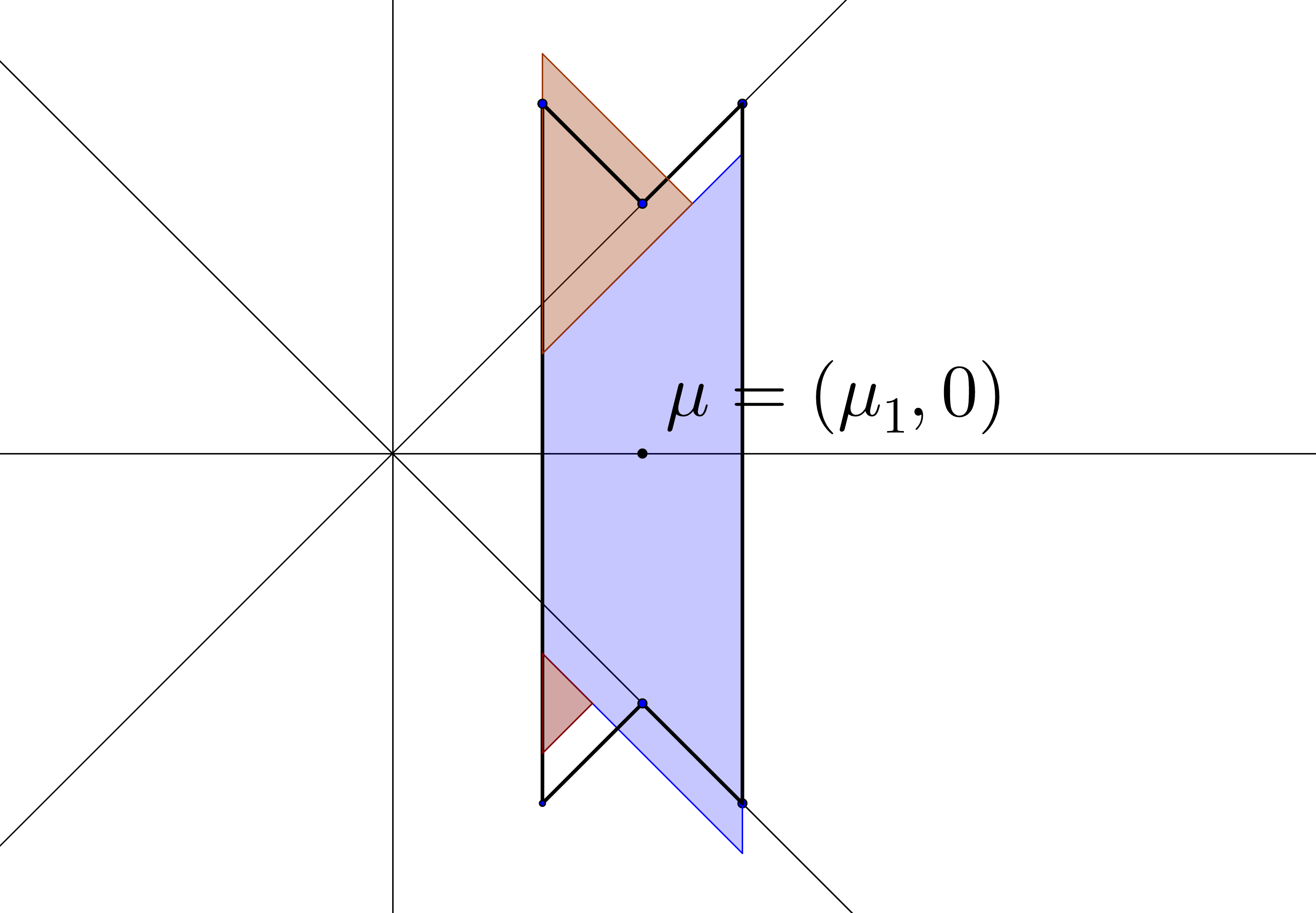
(a)

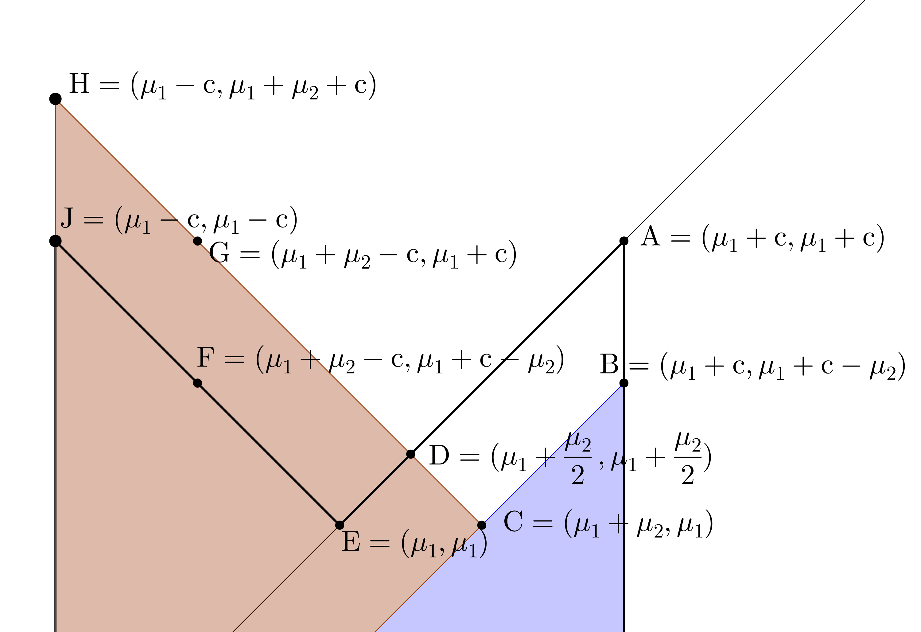
(b)

Figure 9: (a): $B_{(\mu_{1},\mu_{2}),c}$ for $\mu_{1}>c>\mu_{2}$ superposed with $B_{(\mu_{1},0),c}$, after a $\mathbb{P}_{\mu}$-preserving transformations. (b): Detail of the top of panel (a).

Case (3) $c\geq\mu_{1}\geq\mu_{2}$. The only transformation required to compare the probabilities of the regions is to translate $B_{(\mu_{1},\mu_{2}),c}$ to center it at $\left(\mu_{1},0\right)$. See Figure 10. The area of the quadrilateral $EFGH$ in Figure 10(b) is greater than the area of the quadrilateral $ABCD$, and $EFGH$ is closer in norm to $\left(\mu_{1},0\right)$, so $\mathbb{P}_{(\mu_{1},\mu_{2})}\{A_{(\mu_{1},\mu_{2}),c}\}\geq\mathbb{P}_{(\mu_{1},0)}\{A_{(\mu_{1},0),c}\}$.

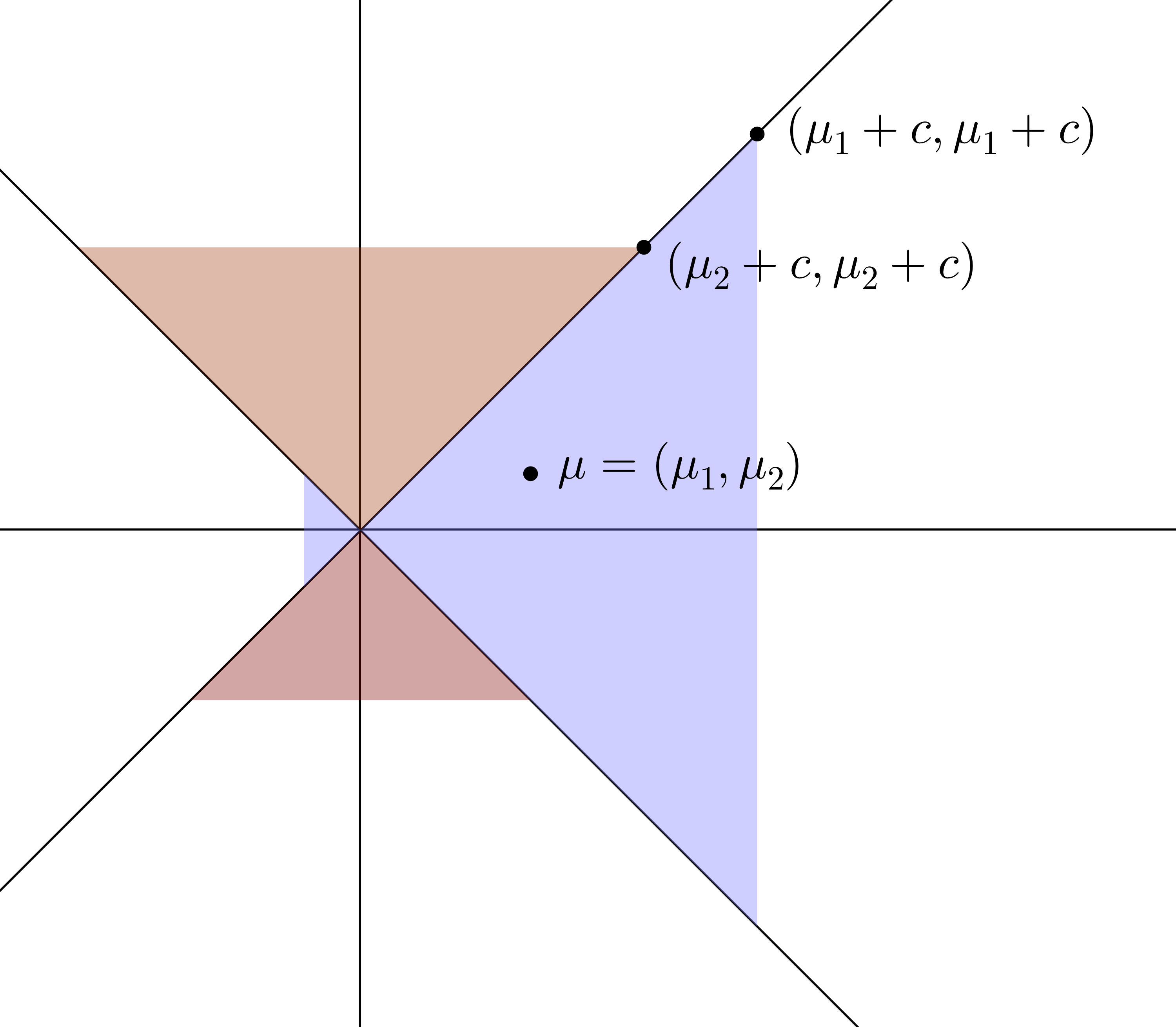
(a)

(b)

Figure 10: $B_{(\mu_{1},\mu_{2}),c}$ and $B_{(\mu_{1},0),c}$ when $c\geq\mu_{1}\geq\mu_{2}$. (a): $B_{(\mu_{1},\mu_{2}),c}$. (b): $B_{(\mu_{1},0),c}$ (the black polygon) and $B_{(\mu_{1},\mu_{2}),c}$ (the shaded polygon) after the translation $h(x)=x-\mu_{2}$.

Appendix B Dependency Simulations

The conditional distribution of the variables selected is stochastically greater than the same variables independently of the selection. This gives rise to the intuition that the method should work under positive dependency. We test the intuition in simulations. Following Cai et al. [2014] we simulate each time $50,000$ observations and consider $m=100$, $k=10$. To demonstrate the methods is applicable when the variables have different distributions, we sample $50$ variables of $Y$ (denoted as $Y_{\left[1:50\right]}$) from multivariate normal $Y_{\left[1:50\right]}\sim\mathcal{N}\left(\theta_{\left[1:50\right]}\cdot\eta,\Sigma\right)$, and $50$ variables (denoted as $Y_{\left[51:100\right]}$) from multivariate $t$ with $5$ degrees of freedom, $Y_{\left[51:100\right]}\sim t_{5}\left(\theta_{\left[51:100\right]}\cdot\eta,\Sigma\right)$. In each simulation we use the same $\Sigma$ for both the normals and the $t$ variables. For all variables, $\theta_{i}\sim\text{Uniform}\left(-1,1\right)$ and $\eta$ transition in the different simulations from $0$ (identically distributed) to $40$ (large differences). We consider three types of $\Sigma$ covariance structures.

1. Auto Regression (AR) matrix such that $\Sigma=\left(\sigma_{i,j}\right)$, and each entry $\sigma_{i,j}=\rho^{\left|i-j\right|}$ for $1\leq i,j\leq m$ and $\rho\in\left\{0.3,0.7\right\}.$

2. Time Decay model (TD) which taken from model $7$ in Cai et al. [2014]. $\Sigma^{\star}=\left(\sigma_{i,j}^{\star}\right)$, $\sigma_{ij}^{\star}=\left|i-j\right|^{-5}/2$ for $j\not=i$. The covariance matrix is $\Sigma=D^{1/2}\Sigma^{\star}D^{1/2}$, where $D=\left(d_{i,j}\right)$, such that $d_{i,j}\sim\text{Uniform}\left(1,3\right).$

3. Block Covariance matrix (Block) - $5$ blocks sized $10$ each, with $\rho\in\left\{0,0.2,0.5,0.75,0.9\right\}.$

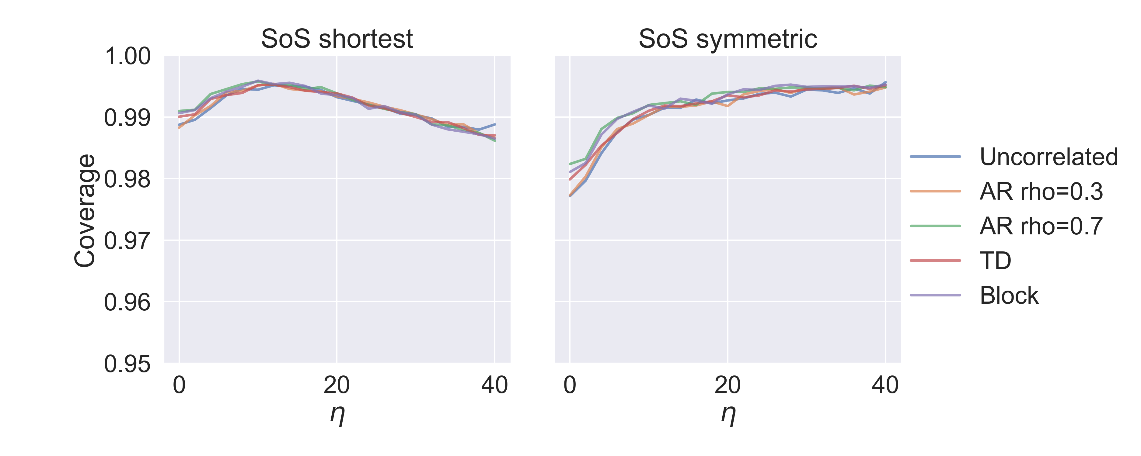
Figure 11: Intervals simultaneous coverage for different dependency structures. The selection of $k=10$ of $m=100$ estimated to be the largest out of $50$ normal and $50$ $t_{5}$ correlated variables for $\alpha=0.05$.

Figure 11 shows the coverage of the SoS shortest and symmetrical intervals with different structures of dependency for $\alpha=0.05$. All intervals obtain the desired coverage and often too conservative, demonstrating the bound might be improved in particular cases. In addition, affect of the different $\Sigma$ is relatively minor and always more conservative. The major affect on the coverage is the selection distribution since the results vary significantly as a function of $\eta$.

References

- Barber and Candès [2015] R. F. Barber and E. J. Candès. Controlling the false discovery rate via knockoffs. The Annals of Statistics, 43(5):2055–2085, 2015.
- Benjamini and Yekutieli [2005] Y. Benjamini and Y. Yekutieli. False discovery rate controlling confidence intervals for selected parameters. J. Am. Stat. Assoc., 100(469):71–80, 2005.
- Berk et al. [2013] R. Berk, L. Brown, A. Buja, K. Zhang, and L. Zhao. Valid post-selection inference. The Annals of Statistics, 41(2):802–837, 2013.
- Braun [1994] H. I. Braun. The collected works of John W. Tukey: Multiple comparisons, 1948-1983. Chapman & Hall, 1994.
- Cai et al. [2014] T. T. Cai, W. Liu, and Y. Xia. Two-sample test of high dimensional means under dependence. Journal of the Royal Statistical Society: Series B (Statistical Methodology), 76(2):349–372, 2014.
- Fithian et al. [2014] W. Fithian, D. Sun, and J. Taylor. Optimal inference after model selection. arXiv preprint arXiv:1410.2597, 2014.
- Fithian et al. [2015] W. Fithian, J. Taylor, R. Tibshirani, and R. Tibshirani. Selective sequential model selection. arXiv preprint arXiv:1512.02565, 2015.
- Fuentes et al. [2018] C. Fuentes, G. Casella, and M. T. Wells. Confidence intervals for the means of the selected populations. Electronic Journal of Statistics, 12(1):58–79, 2018.
- Grimmett and Stirzaker [2001] G. R. Grimmett and D. R. Stirzaker. Probability and Random Processes. Oxford University Press, August 2001. ISBN 0198572220.
- Hechtlinger [2014] Y. Hechtlinger. Confidence interval for the selected. Master’s thesis, Tel Aviv University, Tel Aviv, Israel, June 2014. Available at https://tau-primo.hosted.exlibrisgroup.com/primo-explore/fulldisplay?docid=972TAU_ALMA71237141730004146&context=L&vid=TAU&search_scope=TAU_Blended&tab=default_tab&lang=en_US,.
- Hochberg and Tamhane [1987] Y. Hochberg and A. C. Tamhane. Multiple comparison procedures. Wiley, New York., 1987.
- Hsu [1981] J. Hsu. Simultaneous confidence intervals for all distances from the best. Ann. Stat., 9:1026Ð1034, 1981.
- Hsu [1996] J. Hsu. Multiple Comparisons: Theory and Methods. Chapman and Hall, London, 1996.