Many-body Chaos in Thermalised Fluids

Abstract

Linking thermodynamic variables like temperature $T$ and the measure of chaos, the Lyapunov exponents $\lambda$, is a question of fundamental importance in many-body systems. By using nonlinear fluid equations in one and three dimensions, we show that in thermalised flows $\lambda\propto\sqrt{T}$, in agreement with results from frustrated spin systems. This suggests an underlying universality and provides evidence for recent conjectures on the thermal scaling of $\lambda$. We also reconcile seemingly disparate effects—equilibration on one hand and pushing systems out-of-equilibrium on the other—of many-body chaos by relating $\lambda$ to $T$ through the dynamical structures of the flow.

Many-body chaos is the key mechanism to explain the fundamental basis—thermalisation and equilibration—of statistical physics. However, there are equally important examples in nature, such as turbulence, where chaos plays a role that is seemingly opposite from the settling down through thermalisation and equilibration of several many-body systems. This contrast becomes stark if we argue in terms of the celebrated butterfly effect  Lorenz (1963, 1993, 2000); Hilborn (2004): While the amplification of the wingbeat results in complex dynamical macroscopic structures in driven-dissipative systems (e.g., a turbulent fluid), the same amplification leads to a loss of memory of initial conditions, resulting in ergodic behaviour and eventual thermalisation or equilibration, in Hamiltonian many-body systems. How then do we reconcile these two apparently disparate roles of many-body chaos?

An important piece of the answer lies in investigating the spatio-temporal aspects (the Lyapunov exponent $\lambda$ and butterfly speed $v_{\mathrm{B}}$) of many-body chaos in fluids to reveal its connection with macroscopic (thermodynamic) characterisation of the system. This provides for comparisons of length and time scales of chaos and thermalisation, on the one hand, and the non-linear dynamic structures of the fluid-velocity field on the other.

Characterisations of chaos and its connection with transport and hydrodynamics are recent in the context of both classical and quantum many-body systems like unfrustrated and frustrated Das et al. (2018); Bilitewski et al. (2018, 2021); Ruidas and Banerjee (2020) magnets, strongly correlated field theories Blake (2016); Blake et al. (2017); Gu et al. (2017); Lucas (2017); Werman et al. (2017); Patel et al. (2017); Patel and Sachdev (2017); kit ; Banerjee and Altman (2017)) and field theories of black-holes Shenker and Stanford (2014); Cotler et al. (2017). A common feature responsible for the unconventional signatures of chaos in many of these systems seems to originate from a large set of strongly coupled, dynamic, low energy modes arising from competing interactions. This is similar a turbulent fluid where the triadic interactions of velocity (Fourier) modes across several decades lead to strong couplings resulting in, e.g., scale-by-scale energy transfers Kraichnan (1971); Orszag (1970).

These studies have been facilitated by the development of quantum out-of-time commutators (OTOCs) Larkin and Ovchinnikov (1969); kit ; Maldacena et al. (2016); Das et al. (2018); Roberts and Stanford (2015); Dóra and Moessner (2017); Aleiner et al. (2016) and their classical counterpart the decorrelator Das et al. (2018); Bilitewski et al. (2018) which measure how two very nearly identical copies of a system decorrelate spatio-temporally. The classical decorrelators are invaluable for understanding the butterfly effect Lorenz (1963, 1993, 2000); Hilborn (2004) in non-integrable, chaotic, classical many-body systems through the measurement of $\lambda$ and $v_{\mathrm{B}}$. Since by construction, these OTOCs or decorrelators provide a unified framework to bridge thermodynamic variables (e.g., temperature $T$) with the butterfly effect, they are a unique prescription to connect many-body chaos with the foundations of statistical approaches in both classical and quantum many-body systems. The most striking example of this is that while for quantum systems, $\lambda\leq T/\hbar$, limiting the rate of scrambling Maldacena et al. (2016)), the analogous conjecture for classical systems is $\lambda\propto\sqrt{T}$ at low temperatures Maldacena et al. (2016); Kurchan (2018).

In this Letter, by using a model of thermalised fluids, we derive $\lambda\propto\sqrt{T}$ and demonstrate a possible universality of many-body chaos without an apparent (weakly interacting) quasi-particle description, and hence a Kinetic Theory. Interestingly, we show how decorrelators sense the emergent dynamical structures of the fluid velocity field, providing an elegant way to bridge the ideas of many-body chaos with foundational principles of statistical physics: Thermalisation, equilibration and ergodicity.

For classical systems, recent understanding of spatio-temporal chaos through decorrelators stems primarily from spin systems Bilitewski et al. (2018, 2021); Ruidas and Banerjee (2020) . However, these ideas have not been applied for the most ubiquitous of chaotic, nonlinear, systems: Turbulent flows. This is because, unlike spin-systems, turbulent flows, governed by the viscous Navier-Stokes equation, are an example of a driven-dissipative system without a Hamiltonian or a statistical physics description in terms of thermodynamic variables. Therefore, we look for variations of the Navier-Stokes equation which, whilst preserving the same non-linearity, nevertheless has a a Hamiltonian structure, resulting in a chaotic, thermalised fluid.

Such a prescription leads to the inviscid, three-dimensional (3D) Euler and one-dimensional (1D) Burgers equations, but retaining only a finite number of Fourier modes through a (Fourier) Galerkin truncation Cichowlas et al. (2005); Krstulovic and Brachet (2008); Ray et al. (2011); Majda and Timofeyev (2000). Such a projection of the partial differential equations on to a finite-dimensional sub-space ensures conservation of momentum, energy and phase space, and guarantees chaotic solutions for the flow field which thermalise. These thermalised fluids (see Appendix A) are characterised by energy equipartition and velocity fields with Gibbs distribution $\mathcal{P}[{\bf v}]\leavevmode\nobreak\ d\mathbf{v}=\left(\frac{3}{2\pi E}\right)^{3/2}\exp[-{3\mathbf{v}^{2}}/2E]\leavevmode\nobreak\ d{\bf v}$ as illustrated in Fig. 1. Here $E$ is the conserved energy density of the system satisfying $\left\langle\frac{1}{2}\mathbf{v}^{2}\right\rangle=E$. This allows us to define a temperature, $T=\frac{2}{3}E$ such that the different thermalised configurations describe a canonical ensemble. A thermalised fluid is thus not dissimilar to that of correlated many-body condensed matter systems (e.g., frustrated magnets) where the microscopic memory does not dictate the dynamical correlations.

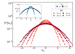
Figure 1: Probability distribution functions of the $x$-component of the thermalised velocity field from Galerkin-truncated 3D Euler and (inset) 1D Burgers simulations for different energies; dashed lines denote the corresponding Gibbs distribution.

These thermalised fluids set the platform for addressing the primary question of the growth of perturbations in a classical, chaotic system. To do this, in the 3D Euler, an arbitrary realisation of the thermalised solution ${\bf v_{0}^{a}}={\bf v}^{\rm th}$ is taken and a second copy generated, with a perturbation in velocity field, ${\bf v_{0}^{b}}={\bf v_{0}^{a}}+\bm{\delta}{\bf v}_{0}$. Here, $\bm{\delta}{\bf v}_{0}=\bm{\nabla}\times\mathbf{A}$, with $A_{i}=\epsilon\sqrt{E}\;r_{0}\exp\left[{-\tfrac{r^{2}}{2r_{0}^{2}}}\right]\hat{e}_{i}$, is an infinitesimal (characterised by $\epsilon\ll 1$) perturbation centred at the origin and which falls off rapidly with distance $r$ (with the reference scale $r_{0}\ll 2\pi$) making it spatially localised.

We now evolve (see Appendix B) the Galerkin-truncated Euler equation, independently for the two copies, with initial conditions ${\bf v_{0}^{a}}$ and ${\bf v_{0}^{b}}$ to obtain (thermalised) solutions ${\bf v^{a}}({\bf x},t)$ and ${\bf v^{b}}({\bf x},t)$ and thence the difference field $\bm{\delta}{\bf v}({\bf x},t)={\bf v^{b}}({\bf x},t)-{\bf v^{a}}({\bf x},t)$. Since initially this difference field $\bm{\delta}{\bf v}({\bf x},0)\equiv\bm{\delta}{\bf v}_{0}$ was spatially localised and vanishingly small, its subsequent spatio-temporal evolution reflects how the butterfly effect manifests itself in such systems. Fundamentally, this is a question of how systems ${\bf a}$ and ${\bf b}$ decorrelate and intimately connected with questions of ergodicity and thermalisation.

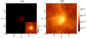
Figure 2: Representative plots of the difference field $|\bm{\delta}\mathbf{v}(\mathbf{x},t)|^{2}$, along the $z=0$ plane of a 3D thermalised fluid (with energy $E=2.0$ and a perturbation amplitude $\epsilon=10^{-6}$ at (a) early ($t=0.4$) and (b) later ($0.7$) times. The inset of panel (a) shows the same early time data, with a magnified scale, to reveal a somewhat self-similar spatial structure that arises from non-local interactions (see main text). See also https://www.youtube.com/watch?v=yRmdvwX5zhE for a time evolution of the difference field.

To make this assessment rigorous, we construct the spatially-resolved decorrelator $\phi({\bf x},t)=\left\langle\frac{1}{2}|\bm{\delta}{\bf v}({\bf x},t)|^{2}\right\rangle$, where $\langle\cdots\rangle$ denotes averaging over configurations taken from the thermalised ensemble and distance is measured from origin where the perturbation is seeded at $t=0$. In Fig. 2 (see, https://www.youtube.com/watch?v=yRmdvwX5zhE for a video of the full evolution) we show the spatial profile (in the $z=0$ plane) of $|\bm{\delta}{\bf v}({\bf x},t)|^{2}$ for a particular initial realisation of systems a and b at two different instants of time. While at very early times $t=0^{+}$, panel (a), $|\bm{\delta}{\bf v}({\bf x},t)|^{2}$ remains small but diffuses instantly and arbitrarily, a more striking behaviour is seen at later times (panel (b)) when the spatial spread is controlled by the strain in the velocity field as we shall see below. (It is likely that that the initial, instantaneous spread is a result of the non-locality (in space) of the 3D fluid because of the pressure term; however since the Galerkin-truncation also introduces an additional non-locality, the precise mechanism for the initial spread is hard to pin down.)

Since the thermalised fluid is statistically isotropic, the decorrelator $\phi(\mathbf{x},t)$ is a function of $|\mathbf{x}|$. We exploit this to construct the more tractable angular-averaged decorrelator $\phi(r,t)=\frac{1}{4\pi r^{2}}\int d\bm{\Omega}_{r}\leavevmode\nobreak\ \phi({\bf x},t)$.

Given the non-locality of the 3D Euler equation, these systems differ crucially from spin systems in the absence of pilot waves and a distinct velocity scale akin to a butterfly speed Das et al. (2018); Bilitewski et al. (2018). Instead, decorrelators for 3D thermalised fluids have a self-similar spatial profile $\phi(r,t)\sim r^{-\alpha}$ (with $\alpha\sim 4$). The lack of a sharp wave-front and self-similarity is evident from Fig. 2(b) and the inset of Fig. 2(a). Therefore to track the temporal evolution of the decorrelator it is convenient to introduce the space-averaged decorrelator $\Phi(t)=\frac{1}{V}\int d^{3}{\bf x}\leavevmode\nobreak\ \phi({\bf x},t)$ which then serve as a diagnostic for the temporal aspects of this problem.

This allows us, starting from the 3D Euler equation, to derive the evolution equation

$$\dot{\Phi}(t)=-\overline{\left\langle\delta v_{i}S_{ij}\delta v_{j}\right\rangle}$$ (1)

in terms of the familiar rate-of-strain tensor $2S_{ij}=\partial_{i}v^{\rm a}_{j}+\partial_{j}v^{\rm a}_{i}$; the over-bar in the definition denotes a spatial average.

By using the eigenbasis of ${\bf S}$, we re-write the above equation as $\dot{\Phi}=-\displaystyle\sum_{i=1}^{3}\>\overline{\left\langle\hat{\alpha}_{i}^{2}\gamma_{i}|\bm{\delta}\mathbf{v}|^{2}\right\rangle}$ where $\left\{\gamma_{i}\right\}$ are the three eigenvalues and $\left\{\hat{\alpha_{i}}\right\}$ are the direction cosines of $\bm{\delta}\mathbf{v}$ along the three eigen-directions. Equation 1, which formally resembles the enstrophy production term for the Euler equation Ashurst et al. (1987); Galanti et al. (1997), is an important result that connects the decorrelator with the dynamical structures of the velocity field.

Our direct numerical simulations (DNSs, see Appendix B) of the truncated 3D Euler equation show strong evidence that the difference fields preferentially grow, at short times, along the compressional eigen-direction ($i=3$) of the thermalised fluid leading to a further simplification $\dot{\Phi}\approx-\overline{\left\langle\hat{\alpha}_{3}^{2}\gamma_{3}|\bm{\delta}\mathbf{v}|^{2}\right\rangle}$. Since by definition $\gamma_{3}<0$, this ensures not only the positive definiteness of $\dot{\Phi}(t)$, but also, since (up to constants) $\dot{\Phi}(t)\sim-\overline{\gamma_{3}}\leavevmode\nobreak\ \Phi$, an exponential growth with a Lyapunov exponent $\lambda\sim|\overline{\gamma_{3}}|$ at short times (Fig. 5). This connects the straining of the flow-field with $\lambda$.

How robust is this short-time behaviour with respect to both dimension and the compressibility of the flow?

The answer lies in an analysis of the 1D (compressible) Burgers equation with $N_{G}$ Fourier modes. Furthermore, to underline the universality of our results, this time we construct the decorrelator and carry out the theoretical (see Appendix C) and numerical analysis entirely in Fourier space. As before, from the thermalised solution (in Fourier space) ${\hat{v}}^{\rm th}$, defining a control field ${\hat{v}}^{\bf a}_{0}={\hat{v}}^{\rm th}$ and a perturbed field ${\hat{v}}_{0}^{\bf b}={\hat{v}}_{0}^{\bf a}(1+\epsilon\delta_{k,k_{p}})$ with large values of the perturbation wave-number $k_{p}$ to generate de-localised small-scale perturbations in the systems (see Appendix B). It is important to stress that given the seed perturbation is localised in Fourier space in 1D (and hence de-localised in physical space), the spatial spread of perturbations, which is relevant and studied for 3D fluids in this Letter, remains outside the scope of analysis here.

As before, both systems are evolved independently and the Fourier space decorrelator $|\hat{\Delta}_{k}|^{2}=\langle|\hat{v}_{k}^{\bf a}-{\hat{v}}^{\bf b}_{k}|^{2}\rangle$, measured, mode-by-mode, as a function of time. Given the relative analytical simplicity of the 1D system, we construct the equation of motion of $|\hat{\Delta}_{k}|^{2}$ and derive an exponential growth of the decorrelator associated with a Lyapunov exponent $\lambda$. Thus the theoretical calculations for the 1D model are not only consistent with the more complex 3D system but also provide, as we see below, a more rigorous insight into how the Lypunov exponent scales with $T$ and the degrees of freedom $N_{G}$ of our system. (See Appendices C – F for the derivation of the linear theories describing the short-time dynamics of the decorrelator.)

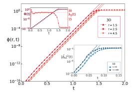
Figure 3: Semi-log plots of $\phi(r,t)$ ($E=1.0$)) and (lower inset) $|\hat{\Delta}_{k}|^{2}$ ($E=2.0$) showing an initial exponential growth and eventual saturation. The dashed lines, from linearised theory, are in excellent agreement with DNSs at early times. (Upper inset) Semi-log (left y-axis) plot of $\Phi(t)$ (3D fluid) along with results from our linearised theory (dashed line). $\lambda$, extracted from $\Phi(t)$, shown as dash-dot horizontal line, agrees well with $\lambda_{S}$ (linearised theory, right y-axis).

At long times, since systems a and b decorrelate $\langle{\bf v^{a}}\cdot{\bf v^{b}}\rangle=0$, leading to suspension of the underlying approximations in the linear theory presented above, $\Phi$ and $|\hat{\Delta}_{k}|^{2}$ must saturate to a value equal to $2E$ and $2E/N_{G}$ respectively.

With these theoretical insights for both the 1D and 3D systems, we test them against results from our numerical simulations. In Fig. 3 we show representative results for $\phi(r,t)$ ($\Phi$ in the upper inset) from 3D Euler and $|\hat{\Delta}_{k}|^{2}$ for the 1D Burgers (lower inset) versus time on a semi-log scale. The symbols (for different values of $r$ and $k$) are results from the full nonlinear DNSs while the dashed lines correspond to decorrelators obtained the linearised theory.

Consistent with our theoretical estimates described above, the decorrelators from the full, nonlinear DNSs (shown by symbols) grow exponentially (positive $\lambda$) before eventually saturating (as the two systems decorrelate) to a value set by the energy. The agreement between these decorrelators and the ones we estimate theoretically through a linearised model (dashed lines) is remarkable during the early-time exponential phase. However, decorrelators constructed from the linearised model (valid for short times) are insensitive to non-linearities and continue growing exponentially, while the ones from the full nonlinear system eventually saturate. We will soon return to the question of time scales which determine this saturation.

Finally, we confirm the validity of Eq. 1 by showing (upper inset, Fig. 3) the agreement between $\lambda_{S}(t)={-\overline{\left\langle\delta v_{i}S_{ij}\delta v_{j}\right\rangle}}/{\Phi(t)}$ and the Lyapunov exponent $\lambda$ extracted from the decorrelator $\Phi(t)$ measured in DNSs. The agreement between the two is almost perfect at short times before $\lambda_{S}(t)$ decays to zero as the decorrelator saturates.

This inevitably leads us to central question of this work: How fast do perturbations grow in a classical, chaotic system and how does it depend on the temperature $T$ as well as the number of modes, $N_{G}$ ? Furthermore is the scaling behaviour of $\lambda$ really universal?

Although non-linear equations for hydrodynamics do not yield easily to an analytical treatment, it is tempting to theoretically estimate the functional dependence of $\lambda$ on $T$ and $N_{G}$. An extensive analysis (see Appendices C – D) of the linearised equations for $\Phi(t)$ and $|\hat{\Delta}_{k}|^{2}$ show that under very reasonable approximations, which were tested against data, $\lambda\propto N_{G}\sqrt{T}$. Whereas for the Euler fluid this scaling is a consequence of the statistics of the strain-rate-tensor which determines the behaviour of $\Phi(t)$, the analogous result for the 1D system is obtained by straightforward algebraic manipulations, factoring in the statistical fluctuations, of the equation governing the evolution of $|\hat{\Delta}_{k}|^{2}$.

Our theoretical prediction is easily tested by measuring $\lambda$ in DNSs of the full non-linear 3D Euler and 1D Burgers equations. From plots such as in Fig. 3, we extract the mean $\lambda$ and its (statistical) error-bar, and examine its dependence on temperature $T$ (and $N_{G}$) by changing the magnitude of the initial conditions and hence the initial energy or temperature. (Surprisingly, $\lambda$ measured through such decorrelators are independent of $r$ or $k$, as was already suggested in Fig. 3.) Figure LABEL:fig:lyapunovOfDecorrelator shows a unified (3D Euler and 1D Burgers) log-log plot of all the rescaled Lyapunov exponent $\lambda/N_{G}$ measured—for different strengths and scales of perturbations and $N_{G}$—as a function of temperature $T$. The collapse of the data on the dashed line, denoting a $\sqrt{T}$ scaling, shows that the many-body chaos of such thermalised fluids is characterised by the behaviour $\lambda\propto N_{G}\sqrt{T}$. It is worth stressing that these DNS results for the 3D Euler equations make the theoretical bound (see Appendix D) sharp.

These, to the best of our knowledge, are the first results, and confirmation of earlier conjectures Kurchan (2018); Maldacena et al. (2016) and demonstrations for classical spin systems Bilitewski et al. (2018), that $\lambda\propto\sqrt{T}$ in a chaotic and non-linear, many-body classical system obeying the equations of hydrodynamics. Remarkably, we also find strong evidence that $\lambda$ scales linearly with $N_{G}$ in such extended systems and independent of spatial dimension and compressibility of the flow.

Given the association of many-body chaos with ergodicity and equilibration in classical statistical physics, how well do measurements of $\lambda$ relate to the (inverse) time scales associated with the loss of memory? The simplest measure of how fast a system forgets is the ensemble-averaged autocorrelation function $C(t)=\left(2E\right)^{-1}\left\langle\mathbf{v}^{\mathrm{th}}(t)\cdot\mathbf{v}^{\mathrm{th}}(0)\right\rangle$ (Fig. 5). It is easy to show (see Appendices C – D) that $C(t)\approxeq\mathrm{exp}\left[-\frac{t^{2}}{2\tau^{2}}\right]$ with an auto-correlation time $\tau\sim 1/\lambda$ as clearly shown from our measurements (upper inset, Fig. 5). This association of $\tau$ with $\lambda$ provides a firm foundation to interpret the salient features of many-body chaos in terms of principles of statistical physics: Ergodicity and thermalisation. A further connection is established through the relation between the time scales $t_{\mathrm{sat}}\sim\tau\sim 1/\lambda$ at which the decorrelator saturates as $\Phi(t)\approxeq\;2E\left(1+\mathrm{exp}\left[-\lambda(t-t_{\mathrm{sat}})\right]\right)^{-1}$.

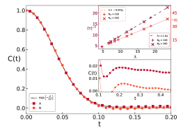
Figure 5: A plot of $C(t)$ for a (A) nearly and (B) completely thermalised 3D fluid along with the theoretical Gaussian prediction. (Lower inset) A magnified view shows that for a fluid which is not completely thermalised, $C(t)$ falls off to zero much more slowly. (Upper inset) Representative plots of $\tau$ and the average (negative) eigen-value (compressional direction) versus $\lambda$.

The generality of the OTOCs and cross-correlators lead to questions of connecting the macroscopic variables with the scales of chaos in the most canonical of chaotic systems: Those described by non-linear equations of hydrodynamics. Here we provide the first evidence of the temperature dependence of the Lyapunov exponent in (continuum) classical non-linear hydrodynamic systems and show its robustness with respect to spatial dimensions and compressibility effects. It is important to underline that many-body chaos and $\lambda\sim N_{G}\sqrt{T}$ is really an emergent feature of a fluid which is thermalised. We checked this explicitly by measuring the decorrelators in the flow before it thermalises and found, despite the conservation laws still holding, no associated exponential growth and spread of the difference field. Furthermore, our measured $\lambda$ should be identified with the largest Lyapunov exponent of the system and that $t_{\mathrm{sat}}$ is a useful estimate of thermalisation (or equilibration) time.

Finally, the temperature dependence of $\lambda$ is consistent with recent results for classical spin liquids without quasi-particles Bilitewski et al. (2018); Scaffidi and Altman (2019); Ruidas and Banerjee (2020); Bilitewski et al. (2021) as well as more general dimensional arguments based on phase-space dynamics Kurchan (2018) of classical many-body systems. In this regard we note that in classical spin-systems Bilitewski et al. (2021), the existence of low energy quasi-particles seems to reduce the chaotic behaviour of the system ($\lambda\propto T^{a},\leavevmode\nobreak\ a>0.5$). While more detailed and theoretical investigation of these features, as well as, how far they are relevant for the spontaneously stochastic Navier-Stokes turbulence are interesting future directions, this butterfly effect for classical, non-linear, hydrodynamic systems seems to be robust and generic.

While it is probably true that the exact nature of the dependence of the Lyapunov exponent on the temperature (or energy density) and number of degrees of freedom should vary from system to system, the evidence we provide of their inter-dependence opens new avenues and questions. In particular, these studies demonstrate the dependence of signatures of spatio-temporal chaos on the thermodynamic variables as well its relation with the transport properties.

Appendix A Appendix A: Thermalised fluids: Galerkin projection of 1D Burgers and 3D Euler Equations

The dynamics of inviscid, ideal fluids satisfy well-known partial differential equations. For the scalar velocity field $u$ in one-dimensional (1D) flows, this is known as the (inviscid) Burgers equation:

$$\frac{\partial u}{\partial t}+\frac{\partial u^{2}}{\partial x}=0$$ (2)

with initial conditions $u_{0}$.

For three-dimensional flows (3D), the analogous equation for the (incompressible) velocity vector ${\bf u}({\bf x},t)$ and scalar pressure $P$ fields satisfy the celebrated Euler equation:

$$\frac{\partial{\bf u}}{\partial t}+{\bf u}.\cdot\nabla{\bf u}=-\nabla P$$ (3)

augmented by the constraint $\nabla\cdot{\bf u}=0$ and initial conditions ${\bf u}_{0}$.

While the 1D inviscid Burgers equation admits real singularities, which manifests itself as pre-shocks and then shocks in the velocity profile at a finite time $t_{\star}$ (Fig. 6(a)) and dissipates energy (even in the absence of a viscous term) Frisch and Bec (2001); Bec and Khanin (2007), the issue of finite-time blow-up for the 3D Euler equation still remains one of the most important, unsolved, problems in the natural sciences. Nevertheless, weak (in the sense of distributions) solutions of the 3D Euler equations have been recently shown to be dissipative as conjectured by Onsager and consistent with the celebrated problem of dissipative anomaly of high Reynolds number turbulence. Therefore, such inviscid, infinite-dimensional partial differential equations, in one or three dimensions (like their viscous counterparts) lack a Hamiltonian structure and cannot lead to solutions characterised by a statistical equilibria.

Fortunately, a subtle, but significant, modification to these equations, while preserving the essential nonlinearity, allows us to move away from the dissipative to thermalised solutions with an energy equipartition and Gibbs distribution of the velocity field. Within the space of $2\pi$ periodic solutions, an expansion of the solution in an infinite Fourier series allows us to define the Galerkin projection as a low-pass filter $\mathrm{P}_{K_{G}}$ which sets all modes with wave vectors $|{\bf k}|>K_{\scriptscriptstyle\mathrm{G}}$, where $K_{\scriptscriptstyle\mathrm{G}}$ is a positive (large) integer, to zero via $\mathrm{P}_{K_{G}}{\bf u}({\bf x})=\sum_{|{\bf k}|\leq K_{\scriptscriptstyle\mathrm{G}}}\mathrm{e}^{\mathrm{i}{\bf k}\cdot{\bf x}}\hat{\bf u_{k}}.$ The truncation wavenumber $K_{\scriptscriptstyle\mathrm{G}}$ sets the number of Fourier modes $N_{G}$ kept and is a measure of the effective number of degree of freedom as well as providing a microscopic (ultraviolet) cut-off for the system. These definitions, without the loss of incompressibility, lead to the Galerkin-truncated Euler equation for the truncated field, written, most conveniently, component-wise in Fourier space ${\hat{v}}_{\alpha}({\bf k})$

$$\frac{\partial{\hat{v}}_{\alpha}({\bf k})}{\partial t}=-\frac{\mathrm{i}}{2}\mathcal{P}_{\alpha\beta\gamma}({\bf k})\sum_{{\bf p}}{\hat{v}}_{\beta}({\bf p}){\hat{v}}_{\gamma}({\bf k}-{\bf p});$$ (4)

where the initial conditions ${\bf v}_{0}=\mathrm{P}_{K_{G}}{\bf u}_{0}$ and the convolution $|{\bf k}\leq K_{\scriptscriptstyle\mathrm{G}}$, $|{\bf p}|\leq K_{\scriptscriptstyle\mathrm{G}}$ and $|{\bf k}-{\bf p}|\leq K_{\scriptscriptstyle\mathrm{G}}$ is constrained via Galerkin truncation. The coefficient ${\mathcal{P}}_{\alpha\beta\gamma}=k_{\beta}P_{\alpha\gamma}+k_{\gamma}P_{\alpha\beta}$, where $P_{\alpha\beta}=\delta_{\alpha\beta}-k_{\alpha}k_{\beta}/k^{2}$ factors in the contribution from the pressure gradient and enforces incompressibility; $\delta_{\alpha\beta}$ is a Kronecker delta.

The same definitions of Galerkin truncation can be extended mutatis mutandis to one dimension, without the additional constraints of incompressibility or pressure gradients, to similarly project the 1D inviscid, $2\pi$-periodic Burgers equation onto the subspace spanned by $K_{\scriptscriptstyle\mathrm{G}}$:

$$\frac{\partial{\hat{v}}(k)}{\partial t}=-\frac{\mathrm{i}k}{2}\sum_{p}{\hat{v}}(p){\hat{v}}(p-k).$$ (5)

With initial conditions $v_{0}$, the Galerkin-truncated Burgers equation also imposes the constraint $k\leq K_{\scriptscriptstyle\mathrm{G}}$, $p\leq K_{\scriptscriptstyle\mathrm{G}}$ and $|p-k|\leq K_{\scriptscriptstyle\mathrm{G}}$ on the convolution.

Thus, beginning with the partial differential equations of ideal fluids in one and three dimensions, Galerkin truncation leads, by self-consistently restricting the velocity field to a finite number of modes $N_{G}$, to a finite-dimensional, nonlinear dynamical systems with a mathematical, nonlinear structure identical to the equations which govern turbulent flows. However, such a truncation, which conserves phase space volume, momentum and kinetic energy, results, through Liouville’s theorem, in solutions at finite times which are in statistical equilibria (unlike the non-equilibrium steady states associated with turbulence) with a characteristic Gibbs distribution and a broadening (standard deviation) $\sigma$ determined by the total (conserved) energy $E$ (Fig. 1, main paper). Thence, a natural association of a temperature $T$ via $T=2\sigma^{2}=2E/3$ for such systems.

Furthermore, it is because of this statistical equilibria that such solutions show an equipartition of kinetic energy amongst all its Fourier modes resulting in, for the 3D problem, an (shell averaged) energy spectrum $E(k)=|{\hat{v}}^{\rm th}({\bf k})|^{2}\propto k^{2}$ Cichowlas et al. (2005) (or, in 1D, $E(k)=|{\hat{v}}^{\rm th}_{k}|^{2}\propto k^{0}$ Ray et al. (2011); Ray (2015); Venkataraman and Ray (2017); Murugan et al. (2020)) at odds with the well known $k^{-5/3}$ spectrum of real turbulence (or $k^{-2}$ in solutions of the Burgers equation in the limit of vanishing viscosity) as clearly shown in Fig. 6(a).

Thus these chaotic systems (in one or three dimensions), rooted in the nonlinear equations of hydrodynamics which form the basis of real turbulence and yet remain in statistical equilibria provides an excellent model for a thermalised fluid. Furthermore, given the conservation of energy and its association with temperature through the Gibbs distribution, it is simple to generate thermalised flows with different temperatures by a simple change in the amplitude of the initial conditions.

Appendix B Appendix B: Direct Numerical Simulations (DNS) of truncated equations

We perform direct numerical simulations (DNSs) of these Galerkin-truncated 3D Euler and the 1D Burgers equations by using a standard pseudo-spectral method with a fourth order Runga-kutta algorithm for time marching. These equations are solved on a $2\pi$ periodic domain with $N^{3}$ for the 3D and $N$ for the 1D equations with a truncation wavenumber $K_{G}$ which results in ${N_{G}}^{3}<N^{3}$ (or, in 1D, $N_{G}<N$) number of degrees of freedom. In our numerical simulations, we have explicitly checked that the kinetic energy is conserved and within a finite time energy equipartition is reached.

For the 3D truncated Euler problem, we begin with an initial kinetic energy spectrum of the form $E(k)=A_{0}k^{4}\exp\left[-\tfrac{k^{2}}{2k_{0}^{2}}\right]$; changing the numerical value of the factor $A_{0}$ allows us to generate thermalised fluid with different energies $E$ and hence temperatures $T$. In our simulations, we use different resolutions $N^{3}=96^{3},128^{3},160^{3},196^{3},224^{3}$ and $256^{3}$ for different values of the truncation wavenumbers $K_{\scriptscriptstyle\mathrm{G}}=N/3,N/4$ and $N/5$ to generate flows with varying degrees of freedom $N_{G}\sim K_{\scriptscriptstyle\mathrm{G}}$ as well as different amplitudes of the initial conditions to scan the temperatures in the range $0.125\leq T\leq 4$, . Our time-step for integration, depending on $K_{\scriptscriptstyle\mathrm{G}}$ and $E$, varies as $\Delta t\lesssim\sqrt{\frac{3}{2E}}\frac{2\pi}{N}$, and the truncated equations were integrated up to a time $t\approx 10$ to generate fully thermalised solution ${\bf v}^{\rm th}$ which provides the starting point to generate systems ${\bf a}$ and ${\bf b}$ used in our calculations of the decorrelator $\Phi(t)$.

For the 1D truncated Burgers problem, we choose an initial condition $v_{0}=A_{0}[\sin x+\sin(2x-0.2)+\sin(5x-0.4)+\sin(7x-0.5)]$; the precise functional form of the initial conditions is immaterial with the total conserved momentum $\int_{0}^{2\pi}v_{0}\leavevmode\nobreak\ dx=0$. Further (as in the 3D problem), changing the numerical constant $A_{0}$, allows us to change the energy $E=\frac{1}{2\pi}\int_{0}^{2\pi}v_{0}^{2}dx=2A_{0}^{2}$ of our system and thence the temperature $2\leq T\leq 18$. Given the lower computational cost for solving the 1D system, we were able use a much larger number of collocation points $N=2^{14}$ to generate systems with larger values of $K_{\scriptscriptstyle\mathrm{G}}=1000$ ($\delta t=10^{-5}$) and 5000 ($\delta t=10^{-6}$) leading to values of $N_{G}$ much larger than those accessible to 3D simulations.

To perturb the system ${\bf a}$, we introduce, for the 3D fluid, a perturbation of strength $\epsilon=10^{-6}$; in the 1D problem, we use $\epsilon=10^{-5}$ and $10^{-4}$. Furthermore, since the perturbation, for the 1D problem, is introduced at wavenumber $k_{p}$ in the Fourier space, we choose different values of $k_{p}=500,900,2500$ and $4000$ to demonstrate the insensitivity of our results to the precise (small) scales of perturbation (and $\epsilon$) as clearly seen in the collapse of the data in Fig. 3 of the main text.

Appendix C Appendix C: Decorrelators: The Linearised Theory

Systems a and b both satisfy the Galerkin-truncated, three-dimensional (3D) Euler equation. Therefore the evolution equation for the difference field $\delta{\bf v}({\bf x},t)={\bf v^{b}}({\bf x},t)-{\bf v^{a}}({\bf x},t)$, component-wise is given by:

$$\partial_{t}\delta v_{i}\left(\mathbf{x},t\right) = -\partial_{j}\left[v_{i}^{\bf a}\delta v_{j}+v_{j}^{\bf a}\delta v_{i}+\delta v_{i}\delta v_{j}\right]$$

$$+ \partial_{ijl}^{3}\displaystyle\int_{\mathcal{D}}d\mathbf{x}^{\prime}\>G(\mathbf{\mathbf{x},\mathbf{x}^{\prime}})\left[v_{j}^{\bf a}\delta v_{l}+v_{l}^{\bf a}\delta v_{j}+\delta v_{j}\delta v_{l}\right]^{\prime};$$

with an initial conditions $\bm{\delta}{\bf v}({\bf x},0)\equiv\bm{\delta}{\bf v}_{0}$ and a Green’s function satisfying $\bm{\nabla}^{2}G(\mathbf{x},\mathbf{x}^{\prime})=\bm{\delta}(\mathbf{x}-\mathbf{x}^{\prime})$. While the non-local and convective terms in this equation clearly suggests that a localised, initial difference $\bm{\delta}{\bf v}({\bf x},0)\equiv\bm{\delta}{\bf v}_{0}$, introduced through the perturbation in b: ${\bf v_{0}^{b}}={\bf v_{0}^{a}}+\bm{\delta}{\bf v}_{0}$; with $\bm{\delta}{\bf v}_{0}=\bm{\nabla}\times\mathbf{A}$, where $A_{i}=\epsilon\sqrt{E}\;r_{0}\exp\left[{-\tfrac{r^{2}}{2r_{0}^{2}}}\right]\hat{e}_{i}$, will de-localise with a spatio-temporal spreading. However, given the nonlinear nature of this equation, estimating how this happens, or more specifically, the temporal growth of the decorrelator $\Phi(t)$ and thence the Lyapunov exponent, is a challenge.

Since the main question which concerns us has to do with the short time growth of these decorrelators, when nonlinear terms $\mathcal{O}(\delta v^{2})$ can be ignored, a reasonable assumption which was validated against data from our Direct Numerical Simulations (DNSs), we linearise Eq. LABEL:evolutionPerturbation:

$$\frac{\partial\delta v_{i}^{\mathrm{lin}}}{\partial t}\approx-v_{j}^{\bf a}\frac{\partial\delta v_{i}^{\mathrm{lin}}}{\partial x_{j}}-\delta v_{j}^{\mathrm{lin}}\frac{\partial v^{\bf a}_{i}}{\partial x_{j}}+\frac{\partial T}{\partial x_{i}};$$ (7)

where, $T=2\delta_{ij}^{2}\int d{\bf y}G(|{\bf x}-{\bf y}|)\delta v_{j}^{\mathrm{lin}}({\bf y})v_{k}^{(a)}({\bf x})$ is the non-local (linear) contribution from the pressure term. It is worth stressing that although we linearise the equation, it still allows for the spatio-temporal spread of the difference field because of its non-local nature. As we have shown in the main paper (Fig. 3; dashed lines), the decorrelator $\Phi(t)$ (or $\phi(r,t)$) obtained from this linearised equation is in agreement, at short times, with those obtained from the DNSs of the full 3D truncated Euler equation. Indeed, quantifying by this agreement through a global relative error:

$$\Gamma(t)=\dfrac{\frac{1}{V}\displaystyle\int_{\mathcal{D}}d\mathbf{x}\frac{1}{2}|\bm{\delta}\mathbf{v}-\bm{\delta}\mathbf{v}^{\mathrm{lin}}|^{2}\>}{\Phi(t)}$$ (8)

where $\mathcal{D}$ is the domain and $V$ the volume of space; in the exponential growth regime $\Gamma\sim 10^{-4}$ and reaches $\mathcal{O}(1)$ at times when the $\Phi(t)$ (or $\phi(r,t)$) obtained from DNSs start to saturate. The linear theory of course fails in this saturation region as the approximations leading upto it no longer holds as $\langle{\bf v^{a}}\cdot{\bf v^{b}}\rangle=0$ and $|\bm{\delta}\mathbf{v}|$ is of the same order as the root-main-squared velocity of the thermalised fluid.

Nevertheless, starting with Eq. LABEL:evolutionPerturbation and taking dot products with $\delta{\bf v}({\bf x},t)$ followed by a spatial integration, we eventually obtain:

$$\dot{\Phi}(t)=-\left\langle\delta v_{i}S_{ij}\delta v_{j}\right\rangle+\left\langle\partial_{j}W_{j}\right\rangle$$ (9)

with

$$W_{j}=-\frac{1}{2}v_{j}^{\bf b}|\bm{\delta}\mathbf{v}|^{2}+\delta v_{j}\partial_{il}^{2}\displaystyle\int_{\mathcal{D}}d\mathbf{x}^{\prime}\>(v_{i}^{\bf a}\delta v_{l}+\delta v_{i}v_{l}^{\bf b})^{\prime}G_{\mathbf{x},\mathbf{x}^{\prime}}$$ (10)

and $S_{ij}$ the familiar rate-of-strain tensor $2S_{ij}=\partial_{i}v^{\bf a}_{j}+\partial_{j}v^{\bf a}_{i}$ for the thermalised fluid. The second, divergence term in Eq. 9 vanishes however because of periodic boundary conditions leading to

$$\dot{\Phi}(t) =-\left\langle\bm{\delta}\mathbf{v}\cdot\mathbf{S}\cdot\bm{\delta}\mathbf{v}\right\rangle$$ (11)

In the main paper, we have illustrated the validity of Eq. 11 in the upper inset of Fig. 5.

Since the rate-of-strain tensor is diagonalisable, in its eigenbasis with eigenvalues $\left\{\gamma_{i}\right\}$ (satisfying the incompressibility constraint $\sum_{i}\gamma_{i}=0$ with extensional $\gamma_{1}>0$ and compressional $\gamma_{3}<0$ eigen-directions) we decompose $\delta{\bf v}$ in the eigenbasis of $S_{ij}$ with (undetermined) components $\alpha_{i}$ along each eigenvector:

$$\dot{\Phi}(t) =-\displaystyle\sum_{i=1}^{3}\>\left\langle\alpha_{i}^{2}\gamma_{i}\right\rangle$$ (12)

Keeping in mind that the thermalised fluid is incompressible and $\dot{\Phi}(t)>0$ at short and $\dot{\Phi}(t)=0$ at long times (saturation), $\alpha_{i}^{2}$ are clearly correlated with the corresponding eigenvectors. Further more, since $\gamma_{3}<0$ and $\dot{\Phi}(t)$ is positive at short times, it seems likely that there must be a preferential alignment of $\bm{\delta}\mathbf{v}$ with the compressional eigenvector.

Theoretically, this idea of preferential alignment is hard to prove. However, we are able to construct from our numerical data the probability distributions of the $\alpha_{i}$ (Fig. 6(b)) for all three eigen-directions and find that the conjectured preferential alignment, namely that the sum in the right hand side of Eq. 12 is dominated by $\gamma_{3}<0$ leading to $\dot{\Phi}>0$, holds.

This allows us to simplify the equation of motion of the decorrelator

$$\dot{\Phi}(t) \sim-\left\langle\alpha_{3}^{2}\gamma_{3}\right\rangle\sim-\overline{\gamma}_{3}\Phi$$ (13)

with $\overline{\gamma}_{3}$ the average (negative) eigenvalue along the compressional direction.

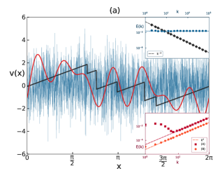
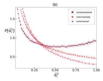
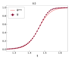
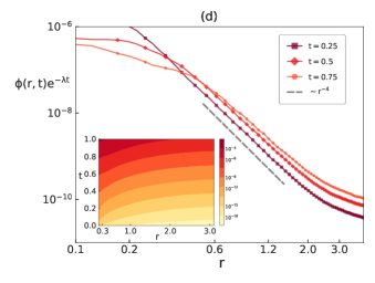
Figure 6: (a) Plots of the Galerkin-truncated Burgers equation velocity field $v$ (blue) and the un-truncated solution $u$ (black) at time $t=10.0$ for an initial condition (red) with $A_{0}=1.0$. The un-truncated or entropy (weak) solution shows clear shocks and the characteristic saw-tooth profile whereas the truncated solution appears as a white noise indicative of a thermalised flow. (Upper Inset) Log-log plots of energy spectrum vs $k$ for the truncated (blue circles) and un-truncated (black squares) equations showing the equipartition of kinetic energy ($E(k)\sim k^{0}$) for the former and a $k^{-2}$ scaling (denoted by a thick black line) for the latter. (Lower Inset) The kinetic energy spectrum of a partially (A, squares; early times) and fully (B, circles; late times) thermalised 3D fluid obtained from simulations of the Galerkin-truncated Euler equation. The dashed lines with a scaling $\sim k^{2}$ is indicative of energy equipartition due to thermalisation. (b) The probability distribution of the components $\hat{\alpha}_{i}^{2}$ for the three eigen-directions clearly suggests the preferential alignment along the direction of compression. (c) A representative plot of the decorrelator $\Phi(t)$ for a 3D thermalised flow ($E=1$) and the empirical form $\overline{\Phi}^{\mathrm{emp}}(t)$ illustrating the approximate agreement between the two. (d) The compensated decorrelator $\phi(r,t)\exp(-\lambda t)$ for different values of $t$ ($E=1$); the grey dashed line shows a scaling $r^{-4}$ is an illustration of the self-similar nature of the spatial spread of the decorrelations. This is confirmed (inset) in the space-time plot of the isocontours of the decorrelator which suggests a spread of the forms $t\sim\ln r$.

For the thermalised fluid emerging from solutions of the Galerkin-truncated 1D Burgers equation, the linearised theory for the decorrelator is relatively straightforward. We recall that beginning with the thermalised solution (in Fourier space) ${\hat{v}}^{\rm th}$ allows us to define a control field ${\hat{v}}^{\bf a}_{0}={\hat{v}}^{\rm th}$ and a perturbed field ${\hat{v}}_{0}^{\bf b}={\hat{v}}_{0}^{\bf a}(1+\epsilon\delta_{k,k_{p}})$ with large values of the perturbation wave-number $k_{p}$ to generate de-localised small-scale perturbations in the system. From this, we define the decorrelator as $|\hat{\Delta}_{k}|^{2}=\langle|\hat{v}_{k}^{\bf a}-{\hat{v}}^{\bf b}_{k}|^{2}\rangle$ or, in physical space, $\Delta=v^{\bf a}-v^{\bf b}$.

Since both fields a and b satisfy the Galerkin-truncated Burgers equation, we can write down the evolution equation:

$$\frac{\partial\Delta}{\partial t}+\mathrm{P}_{\!\!\!{}_{K_{\scriptscriptstyle\mathrm{G}}}}\left[\frac{\partial\Delta v^{\rm th}}{\partial x}+\frac{1}{2}\frac{\partial\Delta^{2}}{\partial x}\right]=0;$$ (14)

with initial conditions, most conveniently defined in Fourier space, as $\hat{\Delta}_{k}(t=0)=\epsilon_{0}{\hat{v}}_{0}^{\rm th}\delta_{k,k_{p}}$ and the projector $\mathrm{P}_{\!\!\!{}_{K_{\scriptscriptstyle\mathrm{G}}}}$ constraining the dynamics on a finite dimensional subspace with a maximum wavenumber ${K_{\scriptscriptstyle\mathrm{G}}}$ and $N_{G}$ degrees of freedom. At short times, we linearise (for the same reasons as outlined for the 3D thermalised fluid) by dropping the quadratic non-linearity of $\Delta$ and obtain estimates, made precise in the next section, of an exponential, $k$-independent growth of $|\hat{\Delta}_{k}|^{2}$ consistent with our findings for the Euler equation. In the main paper, Fig. 3 (inset) shows plots of the decorrelator obtained from our linear theory; the agreement in the exponential phase with the decorrelator obtained from the full DNSs is remarkable. However, as with the 3D thermalised fluid, the approximations which go into the linear theory—dropping of the quadratic term—fails at later times. Hence, while the actual decorrelator measured from simulations of the full nonlinear system saturates, the one obtained from the linear theory continue to grow exponentially.

Appendix D Appendix D: Decorrelators: Bound on the Lyapunov Exponent

The linear theory developed above for the 3D and 1D fluids are not just as useful to predict the nature of decorrelators at early times, but they are indispensable to estimate the Lyapunov exponents and their dependence on both temperature $T$ and degrees of freedom of the system $N_{G}$.

For the 3D thermalised fluid, the linearised theory as summarised in Eq. 13 leads to the following bound on the growth of the decorrelator $\dot{\Phi}(t)\leq-2\overline{\gamma}_{3}\Phi(t)$ and hence the Lyapunov exponent $\lambda\leq-2\overline{\gamma}_{3}$. As we show in the main paper (Fig. 5, upper inset), results from our DNSs confirms this bound as we find $\lambda\approx-0.62\overline{\gamma}_{3}$.

In order to uncover the dependence of $\lambda$ on $T$ and $N_{G}$, we exploit the fact that the linear theory helps us to associate the Lyapunov exponent with the eigenvalues of the strain tensor. Hence, the statistics of this tensor, which depends only on the properties of the velocity field of the thermalised fluid determines the functional form of $\lambda$.

For notational simplicity, we denote $\hat{v}_{i}(\mathbf{k})$ as the Fourier components of the thermalised fluid and estimate:

$$\left\langle\mathrm{Tr}\left[\mathbf{S}^{2}\right]\right\rangle=\left\langle S_{ij}S_{ij}\right\rangle \approx \displaystyle\sum_{\mathbf{k},\mathbf{k}^{\prime}}\>-k_{i}k_{j}^{\prime}\left\langle\hat{v}_{i}(\mathbf{k})\hat{v}_{j}(\mathbf{k}^{\prime})\right\rangle$$ (15)

$$\approx \dfrac{E}{N_{G}^{3}}\displaystyle\sum_{\mathbf{k}}\>k^{2}\approx EN_{G}^{2}$$

leading to $\lambda\sim N_{G}\sqrt{T}$.

For the 1D problem, a similar estimate is obtained by simpler manipulations of the linearised evolution equation for the decorrelator $|\hat{\Delta}_{k}|^{2}$:

$$\frac{\partial|\hat{\Delta}_{k}|^{2}}{\partial t}-\frac{\sqrt{T}}{N_{G}}\sum_{q=1}^{N_{G}}q\left[\hat{\Delta}_{q}\hat{\Delta}_{-k}+\hat{\Delta}_{-k}\hat{\Delta}_{-k-q}\right]=0.$$ (16)

We have confirmed, numerically, that at short times $\hat{\Delta}_{q}\hat{\Delta}_{k}$ remains spectrally flat, i.e., $\hat{\Delta}_{q}\hat{\Delta}_{k}\propto|\Delta_{k}|^{2}$, up to some undetermined numerical constant. Hence, and by using the identity $\sum_{q=1}^{N_{G}}q\approx N_{G}^{2}$ (for large $N_{G}$), we obtain (where $C$ is a numerical constant) $|\Delta_{k}|^{2}\propto e^{CN_{G}\sqrt{T}t}$ and thus, just like for the 3D thermalised fluid, $\lambda\sim N_{G}\sqrt{T}$.

In the main paper, Fig. 4 has plots of the Lyapunov exponents from our DNSs for both 1D and 3D thermalised fluids which confirms the validity of our theoretical estimate.

Appendix E Appendix E: Decorrelators – Saturation

While we do understand why and at what time scales $t_{\mathrm{sat}}$ the decorrelators of thermalised fluids saturate (Fig. 3), it still remains to be understood how they approach the saturated value. To understand this for the 3D thermalised fluid, for simplicity, we define a normalised decorelator $\overline{\Phi}(t)=\frac{\Phi(t)}{2E}$. Given that the only time scale in the problem is the inverse of the Lyapunov exponent, we construct the following empirical form :

$$\overline{\Phi}^{\mathrm{emp}}(t) =\left(1+\mathrm{exp}\left[-\lambda(t-t_{\mathrm{sat}})\right]\right)^{-1}$$ (17)

with a saturation time-scale $t_{\mathrm{sat}}\sim 1/\lambda$ but found more precisely by fitting the data from our simulations. In Fig. 6(c) we show a representative plot illustrating how the empirical form approximately fits the data.

While the functional form of the decorrelator $\overline{\Phi}(t)$ defined above is purely heuristic it does serve to underline the fact that the nature of many-body chaos is determined solely by the Lyapunov exponent.

Appendix F Appendix F: Decorrelators – Spatial Spread

Non-locality is inherent in 3D thermalised flows due to the pressure term as well as Galerkin truncation. Hence it allows the perturbation seeded locally at $t=0$ to affect the evolution of thermalised velocity everywhere. This is already seen in Eq. LABEL:evolutionPerturbation which shows that at $t=0^{+}$, at spatial points far from the center of perturbation, the growth of $\bm{\delta}\mathbf{v}(\mathbf{x})$ is essentially triggered by the non-local integral term. The subsequent growth of the difference field is then through its coupling with the rate-of-strain tensor.

All of this suggest that the spatially resolved decorrelator $\phi(r,t)$ will not have a wavefront which propagates (radially) with a finite butterfly speed. On the contrary, as was also suggested in the inset of Fig. 2(a) in the main paper, one should expect a self-similar spatial profile for decorrelator, i.e., $\phi(r,t)\sim r^{-\alpha}$.

In Fig. 6(d), we see clear evidence of $\phi(r,t)\sim r^{-\alpha}$, with $\alpha\approxeq 4$, for in the range $0\ll r\ll\pi$ (where $\pi$ is half the system size since the perturbation is seeded in the middle of a 2$\pi^{3}$ cubic box). A further consequence of this (Fig. 6(d), inset) is that the isocontours of the decorrelator (measured through a suitable threshold value $\phi_{0}$) are spread in space-time as $t\sim\ln r$.

While we do not have a way of obtaining the exponent $\alpha\approxeq 4$ analytically, the constraint that $\Phi(t)=\displaystyle\int_{0}^{L}dr\>r^{2}\phi(r,t)$ must be bounded (from above) suggests that $\alpha>3$ which is consistent with what we measure in our data.

Given that for the 1D Burgers problem, we carry out the analysis entirely in Fourier space, the seed perturbation is also introduced in Fourier space and hence not localised in physical space. Therefore the question of the spatial spread of decorrelators remains unanswered for 1D thermalised fluids in this study.

References

- Lorenz (1963) Edward N Lorenz, “Deterministic nonperiodic flow,” Journal of the atmospheric sciences 20, 130–141 (1963).
- Lorenz (1993) Edward N Lorenz, The essence of chaos (University of Washington Press, Seattle, Washington, 1993).
- Lorenz (2000) Edward Lorenz, “The butterfly effect,” World Scientific Series on Nonlinear Science Series A 39, 91–94 (2000).
- Hilborn (2004) Robert C Hilborn, “Sea gulls, butterflies, and grasshoppers: A brief history of the butterfly effect in nonlinear dynamics,” American Journal of Physics 72, 425–427 (2004).
- Das et al. (2018) Avijit Das, Saurish Chakrabarty, Abhishek Dhar, Anupam Kundu, David A. Huse, Roderich Moessner, Samriddhi Sankar Ray, and Subhro Bhattacharjee, “Light-Cone Spreading of Perturbations and the Butterfly Effect in a Classical Spin Chain,” Phys. Rev. Lett. 121, 024101 (2018).
- Bilitewski et al. (2018) Thomas Bilitewski, Subhro Bhattacharjee, and Roderich Moessner, “Temperature dependence of the butterfly effect in a classical many-body system,” Phys. Rev. Lett. 121, 250602 (2018).
- Bilitewski et al. (2021) Thomas Bilitewski, Subhro Bhattacharjee, and Roderich Moessner, “Classical many-body chaos with and without quasiparticles,” Phys. Rev. B 103, 174302 (2021).
- Ruidas and Banerjee (2020) Sibaram Ruidas and Sumilan Banerjee, “Many-body chaos and anomalous diffusion across thermal phase transitions in two dimensions,” arXiv preprint arXiv:2007.12708 (2020).
- Blake (2016) Mike Blake, “Universal Charge Diffusion and the Butterfly Effect in Holographic Theories,” Phys. Rev. Lett. 117, 091601 (2016).
- Blake et al. (2017) Mike Blake, Richard A. Davison, and Subir Sachdev, “Thermal diffusivity and chaos in metals without quasiparticles,” Phys. Rev. D 96, 106008 (2017).
- Gu et al. (2017) Yingfei Gu, Andrew Lucas, and Xiao-Liang Qi, “Energy diffusion and the butterfly effect in inhomogeneous Sachdev-Ye-Kitaev chains,” SciPost Phys. 2, 018 (2017).
- Lucas (2017) A. Lucas, “Constraints on hydrodynamics from many-body quantum chaos,” ArXiv e-prints (2017), arXiv:1710.01005 [hep-th] .
- Werman et al. (2017) Y. Werman, S. A. Kivelson, and E. Berg, “Quantum chaos in an electron-phonon bad metal,” ArXiv e-prints (2017), arXiv:1705.07895 [cond-mat.str-el] .
- Patel et al. (2017) Aavishkar A. Patel, Debanjan Chowdhury, Subir Sachdev, and Brian Swingle, “Quantum Butterfly Effect in Weakly Interacting Diffusive Metals,” Phys. Rev. X 7, 031047 (2017).
- Patel and Sachdev (2017) Aavishkar A. Patel and Subir Sachdev, “Quantum chaos on a critical fermi surface,” Proceedings of the National Academy of Sciences 114, 1844–1849 (2017), http://www.pnas.org/content/114/8/1844.full.pdf .
- (16) A. Y. Kitaev, KITP Program: Entanglement in Strongly- Correlated Quantum Matter (2015).
- Banerjee and Altman (2017) Sumilan Banerjee and Ehud Altman, “Solvable model for a dynamical quantum phase transition from fast to slow scrambling,” Phys. Rev. B 95, 134302 (2017).
- Shenker and Stanford (2014) Stephen H. Shenker and Douglas Stanford, “Black holes and the butterfly effect,” Journal of High Energy Physics 2014, 67 (2014).
- Cotler et al. (2017) Jordan S. Cotler, Guy Gur-Ari, Masanori Hanada, Joseph Polchinski, Phil Saad, Stephen H. Shenker, Douglas Stanford, Alexandre Streicher, and Masaki Tezuka, “Black holes and random matrices,” Journal of High Energy Physics 2017, 118 (2017).
- Kraichnan (1971) Robert H. Kraichnan, “Inertial-range transfer in two- and three-dimensional turbulence,” Journal of Fluid Mechanics 47, 525–535 (1971).
- Orszag (1970) Steven A. Orszag, “Analytical theories of turbulence,” Journal of Fluid Mechanics 41, 363–386 (1970).
- Larkin and Ovchinnikov (1969) A. I. Larkin and Y. N. Ovchinnikov, “Quasiclassical Method in the Theory of Superconductivity,” Soviet Journal of Experimental and Theoretical Physics 28, 1200 (1969).
- Maldacena et al. (2016) Juan Maldacena, Stephen H. Shenker, and Douglas Stanford, “A bound on chaos,” Journal of High Energy Physics 2016, 106 (2016).
- Roberts and Stanford (2015) Daniel A. Roberts and Douglas Stanford, “Diagnosing Chaos Using Four-Point Functions in Two-Dimensional Conformal Field Theory,” Phys. Rev. Lett. 115, 131603 (2015).
- Dóra and Moessner (2017) Balázs Dóra and Roderich Moessner, “Out-of-Time-Ordered Density Correlators in Luttinger Liquids,” Phys. Rev. Lett. 119, 026802 (2017).
- Aleiner et al. (2016) Igor L. Aleiner, Lara Faoro, and Lev B. Ioffe, “Microscopic model of quantum butterfly effect: Out-of-time-order correlators and traveling combustion waves,” Annals of Physics 375, 378–406 (2016).
- Kurchan (2018) Jorge Kurchan, “Quantum bound to chaos and the semiclassical limit,” Journal of Statistical Physics 171, 965–979 (2018).
- Cichowlas et al. (2005) Cyril Cichowlas, Pauline Bonaïti, Fabrice Debbasch, and Marc Brachet, “Effective dissipation and turbulence in spectrally truncated euler flows,” Phys. Rev. Lett. 95, 264502 (2005).
- Krstulovic and Brachet (2008) Giorgio Krstulovic and Marc-Etienne Brachet, “Two-fluid model of the truncated euler equations,” Physica D: Nonlinear Phenomena 237, 2015 – 2019 (2008).
- Ray et al. (2011) Samriddhi Sankar Ray, Uriel Frisch, Sergei Nazarenko, and Takeshi Matsumoto, “Resonance phenomenon for the galerkin-truncated burgers and euler equations,” Phys. Rev. E 84, 016301 (2011).
- Majda and Timofeyev (2000) A. J. Majda and I. Timofeyev, “Remarkable statistical behavior for truncated burgers-hopf dynamics,” Proceedings of the National Academy of Sciences of the United States of America 97, 12413–12417 (2000).
- Ashurst et al. (1987) Wm. T. Ashurst, A. R. Kerstein, R. M. Kerr, and C. H. Gibson, “Alignment of vorticity and scalar gradient with strain rate in simulated navier–stokes turbulence,” The Physics of Fluids 30, 2343–2353 (1987), https://aip.scitation.org/doi/pdf/10.1063/1.866513 .
- Galanti et al. (1997) B Galanti, J D Gibbon, and M Heritage, “Vorticity alignment results for the three-dimensional euler and navier - stokes equations,” Nonlinearity 10, 1675–1694 (1997).
- Scaffidi and Altman (2019) Thomas Scaffidi and Ehud Altman, “Chaos in a classical limit of the sachdev-ye-kitaev model,” Phys. Rev. B 100, 155128 (2019).
- Frisch and Bec (2001) U Frisch and J Bec, “Les houches 2000: New trends in turbulence,” (2001).
- Bec and Khanin (2007) Jérémie Bec and Konstantin Khanin, “Burgers turbulence,” Phys. Rep. 447, 1 – 66 (2007).
- Ray (2015) Samriddhi Sankar Ray, “Thermalized solutions, statistical mechanics and turbulence: An overview of some recent results,” Pramana 84, 395–407 (2015).
- Venkataraman and Ray (2017) Divya Venkataraman and Samriddhi Sankar Ray, “The onset of thermalization in finite-dimensional equations of hydrodynamics: insights from the burgers equation,” Proc. Royal Soc. A 473, 20160585 (2017).
- Murugan et al. (2020) Sugan D. Murugan, Uriel Frisch, Sergey Nazarenko, Nicolas Besse, and Samriddhi Sankar Ray, “Suppressing thermalization and constructing weak solutions in truncated inviscid equations of hydrodynamics: Lessons from the burgers equation,” Phys. Rev. Research 2, 033202 (2020).