On the Fairness of Disentangled Representations

Abstract

Recently there has been a significant interest in learning disentangled representations, as they promise increased interpretability, generalization to unseen scenarios and faster learning on downstream tasks. In this paper, we investigate the usefulness of different notions of disentanglement for improving the fairness of downstream prediction tasks based on representations. We consider the setting where the goal is to predict a target variable based on the learned representation of high-dimensional observations (such as images) that depend on both the target variable and an unobserved sensitive variable. We show that in this setting both the optimal and empirical predictions can be unfair, even if the target variable and the sensitive variable are independent. Analyzing the representations of more than $12\,600$ trained state-of-the-art disentangled models, we observe that several disentanglement scores are consistently correlated with increased fairness, suggesting that disentanglement may be a useful property to encourage fairness when sensitive variables are not observed.

1 Introduction

In representation learning, observations are often assumed to be samples from a random variable ${\mathbf{x}}$ which is generated by a set of unobserved factors of variation ${\mathbf{z}}$ [6, 14, 53, 89]. Informally, the goal of representation learning is to find a transformation $r({\mathbf{x}})$ of the data which is useful for different downstream classification tasks [6]. A recent line of work argues that disentangled representations offer many of the desired properties of useful representations. Indeed, isolating each independent factor of variation into the independent components of a representation vector should make it both interpretable and simplify downstream prediction tasks [6, 7, 29, 35, 56, 58, 60, 74, 82, 87, 89, 90, 1, 28].

Previous work [54, 61] has alluded to a possible connection between the motivations of disentanglement and fair machine learning. Given the societal relevance of machine-learning driven decision processes, fairness has become a highly active field [4]. Assuming the existence of a complex causal graph with partially observed and potentially confounded observations [48], sensitive protected attributes (e.g. gender, race, etc) can leak undesired information into a classification task in different ways. For example, the inherent assumptions of the algorithm might cause discrimination towards protected groups, the data collection process might be biased or the causal graph itself might allow for unfairness because society is unfair [5, 11, 68, 73, 75, 83]. The goal of fair machine learning algorithms is to predict a target variable ${\mathbf{y}}$ through a classifier $\hat{\mathbf{y}}$ without being biased by some sensitive factors ${\mathbf{s}}$. The negative impact of ${\mathbf{s}}$ in terms of discrimination within the classification task can be quantified using a variety of fairness notions, such as demographic parity [10, 97], individual fairness [21], equalized odds or equal opportunity [34, 94], and concepts based on causal reasoning [48, 55].

In this paper, we investigate the downstream usefulness of disentangled representations through the lens of fairness. For this, we consider the standard setup of disentangled representation learning, in which observations are the result of an (unknown) mixing mechanism of independent ground-truth factors of variation as depicted in Figure 1. To evaluate the learned representations $r({\mathbf{x}})$ of these observations, we assume that the set of ground-truth factors of variation include both a target factor ${\mathbf{y}}$, which we would like to predict from the learned representation, and an underlying sensitive factor ${\mathbf{s}}$, which we want to be fair to in the sense of demographic parity [10, 97], i.e. such that $p(\hat{\mathbf{y}}=y|{\mathbf{s}}=s_{1})=p(\hat{\mathbf{y}}=y|{\mathbf{s}}=s_{2})\ \forall y,s_{1},s_{2}$. The key difference to prior work is that in this setting one never observes the sensitive variable ${\mathbf{s}}$ nor the other factors of variation except the target variable, which is itself only observed when learning the model for the downstream task. This setup is relevant when sensitive variables may not be recorded due to privacy reasons. Examples include learning general-purpose embeddings from a large number of images or building a world model based on video input of a robot.

Figure 1: Causal graph and problem setting. We assume the observations ${\mathbf{x}}$ are manifestations of independent factors of variation. We aim at predicting the value of some factors of variation ${\mathbf{y}}$ without being influenced by the unobserved sensitive variable ${\mathbf{s}}$. Even though target and sensitive variable are in principle independent, they are entangled in the observations by an unknown mixing mechanism. Our goal for fair representation learning is to learn a good representation $r({\mathbf{x}})$ so that any downstream classifier will be both accurate and fair. Note that the representation is learned without supervision and when training the classifier we do not observe and do not know which variables are sensitive.

Our key contributions can be summarized as follows:

• We motivate the setup of Figure 1 and discuss how general-purpose representations can lead to unfair predictions. In particular, we show theoretically that predictions can be unfair even if we use the Bayes optimal classifier and if the target variable and the sensitive variable are independent. Furthermore, we motivate why disentanglement in the representation may encourage fairness of the downstream prediction models.

• We evaluate the demographic parity of more than $90\,000$ downstream prediction models trained on more than $10\,000$ state-of-the-art disentangled representations on seven different data sets. Our results indicate that there are considerable dissimilarities between different representations in terms of fairness, indicating that the representation used matters.

• We relate the fairness of the representations to six different disentanglement scores of the same representations and find that disentanglement, in particular when measured using the DCI Disentanglement score [22], appears to be consistently correlated with increased fairness.

• We further investigate the relationship between fairness, the performance of the downstream models and the disentanglement scores. The fairness of the prediction also appears to be correlated to the accuracy of the downstream predictions, which is not surprising given that downstream accuracy is correlated with disentanglement.

Roadmap:

In Section 2, we briefly review the state-of-the-art approaches to extract and evaluate disentangled representations. In Section 3, we highlight the role of the unknown mixing mechanism on the fairness of the classification. In Section 4, we describe our experimental setup and empirical findings. In Section 5 we briefly review the literature on disentanglement and fair representation learning. In Section 6, we discuss our findings and their implications.

2 Background on learning disentangled representations

Consider the setup shown in Figure 1 where the observations ${\mathbf{x}}$ are caused by $k$ independent sources $z_{1},\ldots,z_{k}$. The generative model takes the form of [71]:

$$p({\mathbf{x}},{\mathbf{z}})=p({\mathbf{x}}\mid{\mathbf{z}})\prod_{i}p(z_{i}).$$

Informally, disentanglement learning treats the generative mechanisms as latent variables and aims at finding a representation $r({\mathbf{x}})$ with independent components where a change in a dimension of ${\mathbf{z}}$ corresponds to a change in a dimension of $r({\mathbf{x}})$ [6]. This intuitive definition can be formalized in a topological sense [35] and in the causality setting [87]. A large number of disentanglement scores measuring different aspects of disentangled representations have been proposed in recent years.

Disentanglement scores. The BetaVAE score [36] measures disentanglement by training a linear classifier to predict the index of a fixed factor of variation from the representation. The FactorVAE score [49] corrects a failure case of the BetaVAE score using a majority vote classifier on the relative variance of each dimension of $r({\mathbf{x}})$ after intervening on ${\mathbf{z}}$. The Mutual Information Gap (MIG) [13] computes for each factor of variation the normalized gap on the top two entries in the matrix of pairwise mutual information between ${\mathbf{z}}$ and $r({\mathbf{x}})$. The Modularity [79] measures if each dimension of $r({\mathbf{x}})$ depends on at most one factor of variation using the matrix of pairwise mutual information between factors and representation dimensions. The Disentanglement metric of [22] (which we call DCI Disentanglement following [61]) is based on the entropy of the probability that a dimension of $r({\mathbf{x}})$ is useful for predicting ${\mathbf{z}}$. This probability can be estimated from the feature importance of a random forest classifier. Finally, the SAP score [54] computes the average gap in the classification error of the two most predictive latent dimensions for each factor.

Unsupervised methods. State-of-the-art approaches for unsupervised disentanglement learning are based on representations learned by VAEs [51]. For the representation to be disentangled, the loss is enriched with a regularizer that encourages structure in the aggregate encoder distribution [2, 14, 13, 24, 36, 49, 65]. In causality, it is often argued that the true generative model is the simplest factorization of the distribution of the variables in the causal graph [74]. Under this hypothesis, $\beta$-VAE [36] and AnnealedVAE [9] limit the capacity of the VAE bottleneck so that it will be forced to learn disentangled representations. The Factor-VAE [49] and $\beta$-TCVAE [13] enforce that the aggregate posterior $q({\mathbf{z}})$ is factorial by penalizing its total correlation. The DIP-VAE [54] and approach of [65] introduce a “disentanglement prior” for the aggregated posterior. We refer to Appendix B of [61] and Section 3 of [89] for a more detailed description of these regularizers.

3 The dangers of general purpose representations for fairness

Our goal in this paper is to understand how disentanglement impacts the fairness of general purpose representations. For this reason, we put ourselves in the simple setup of Figure 1 where we assume that the observations ${\mathbf{x}}$ depend on a set of independent ground-truth factors of variation through an unknown mixing mechanism. The key goal behind general purpose representations is to learn a vector valued function $r({\mathbf{x}})$ that allows us to solve many downstream tasks that depend on the ground-truth factors of variation. From a representation learning perspective, a good representation should thus extract most of the information on the factors of variation [6], ideally in a way that enables easy learning from that representation, i.e., with few samples.

As one builds machine learning models for different tasks on top of such general purpose representations, it is not clear how the properties of the representations relate to the fairness of the predictions. In particular, for different downstream prediction tasks, there may be different sensitive variables that we would like to be fair to. This is modeled in our setting of Figure 1 by allowing one ground-truth factor of variation to be the target variable ${\mathbf{y}}$ and another one to be the sensitive variable ${\mathbf{s}}$.

There are two key differences to prior setups in the fairness literature: First, we assume that one only observes the observations ${\mathbf{x}}$ when learning the representation $r({\mathbf{x}})$ and the target variable ${\mathbf{y}}$ only when solving the downstream classification task. The sensitive variable ${\mathbf{s}}$ and the remaining ground-truth factors of variation are not observed. We argue that this is an interesting setting because for many large scale data sets labels may be scarce. Furthermore, if we can be fair with respect to unobserved but independent ground-truth factors of variation – for example by using disentangled representations, this might even allow us to avoid biases for sensitive factors that we are not aware of. The second difference is that we assume that the target variable ${\mathbf{y}}$ and the sensitive variable ${\mathbf{s}}$ are independent. While beyond the scope of this paper, it would be also interesting to study the setting where ground-truth factors of variations are dependent.

Why can representations be unfair in this setting? Despite the fact that the target variable ${\mathbf{y}}$ and the sensitive variable ${\mathbf{s}}$ are independent may seem like a overly restrictive assumption, we argue that even in this setting fairness is non-trivial to achieve. Since we only observe ${\mathbf{x}}$ or the learned representations $r({\mathbf{x}})$, the target variable ${\mathbf{y}}$ and the sensitive variable ${\mathbf{s}}$ may be conditionally dependent. If we now train a prediction model based on ${\mathbf{x}}$ or $r({\mathbf{x}})$, there is no guarantee that predictions will be fair with respect to ${\mathbf{s}}$.

There are additional considerations: first, the following theorem shows that the fairness notion of demographic parity may not be satisfied even if we find the optimal prediction model (i.e., $p(\hat{\mathbf{y}}|{\mathbf{x}})=p({\mathbf{y}}|{\mathbf{x}})$) on entangled representations (for example when the representations are the identity function, i.e. $r({\mathbf{x}})={\mathbf{x}}$).

Theorem 1.

If ${\mathbf{x}}$ is entangled with ${\mathbf{s}}$ and ${\mathbf{y}}$, the use of a perfect classifier for $\hat{\mathbf{y}}$, i.e., $p(\hat{\mathbf{y}}|{\mathbf{x}})=p({\mathbf{y}}|{\mathbf{x}})$, does not imply demographic parity, i.e., $p(\hat{\mathbf{y}}=y|{\mathbf{s}}=s_{1})=p(\hat{\mathbf{y}}=y|{\mathbf{s}}=s_{2}),\forall y,s_{1},s_{2}$.

The proof is provided in Appendix A. While this result provides a worst-case example, it should be interpreted with care. In particular, such instances may not allow for good and fair predictions regardless of the representations and real world data may satisfy additional assumptions not satisfied by the provided counter example.

Second, the unknown mixing mechanism that relates ${\mathbf{y}}$, ${\mathbf{s}}$ to ${\mathbf{x}}$ may be highly complex and in practice the downstream learned prediction model will likely not be equal to the theoretically optimal prediction model $p(\hat{\mathbf{y}}|r({\mathbf{x}}))$. As a result, the downstream prediction model may be unable to properly invert the unknown mixing mechanism and successfully separate ${\mathbf{y}}$ and ${\mathbf{s}}$, in particular as it may not be incentivized to do so. Finally, implicit biases and specific structures of the downstream model may interact and lead to different overall predictions for different sensitive groups in ${\mathbf{s}}$.

Why might disentanglement help?

The key idea why disentanglement may help in this setting is that disentanglement promises to capture information about different generative factors in different latent dimensions. This limits the mutual information between different code dimensions and encourages the predictions to depend only on the latent dimensions corresponding to the target variable and not to the one corresponding to the sensitive ground-truth factor of variation. More formally, in the context of Theorem 1, consider a disentangled representation where the two factors of variations ${\mathbf{s}}$ and ${\mathbf{y}}$ are separated in independent components (say $r({\mathbf{x}})_{y}$ only depends on ${\mathbf{y}}$ and $r({\mathbf{x}})_{s}$ on ${\mathbf{s}}$). Then, the optimal classifier can learn to ignore the part of its input which is independent of ${\mathbf{y}}$ since $p(\hat{\mathbf{y}}|r({\mathbf{x}}))=p({\mathbf{y}}|r({\mathbf{x}}))=p({\mathbf{y}}|r({\mathbf{x}})_{y},r({\mathbf{x}})_{s})=p({\mathbf{y}}|r({\mathbf{x}})_{y})$ as ${\mathbf{y}}$ is independent from $r({\mathbf{x}})_{s}$. While such an optimal classifier on the representation $r({\mathbf{x}})$ might be fairer than the optimal classifier on the observation ${\mathbf{x}}$, it may also have a lower prediction accuracy.

4 Do disentangled representations matter?

Experimental conditions

We adopt the setup of [61], which offers the most extensive benchmark comparison of disentangled representations to date. Their analysis spans seven datasets: in four of them (dSprites [36], Cars3D [78], SmallNORB [59] and Shapes3D [49]), a deterministic function of the factors of variation is incorporated into the mixing process; they further introduce three additional variants of dSprites, Noisy-dSprites, Color-dSprites, and Scream-dSprites. In the latter datasets, the mixing mechanism contains a random component that takes the form of noisy pixels, random colors and structured backgrounds from the scream painting. Each of these seven datasets provides access to the generative model for evaluation purposes. Our experimental pipeline works in three stages. First, we take the $12\,600$ pre-trained models of [61], which cover a large number of hyperparameters and random seeds for the most prominent approaches: $\beta$-VAE, AnnealedVAE, Factor-VAE, $\beta$-TCVAE, DIP-VAE-I and II. These methods are trained on the raw data without any supervision. Details on architecture, hyperparameter, implementation of the methods can be found in Appendices B, C, G, and H of [61]. In the second stage, we assume to observe a target variable ${\mathbf{y}}$ that we should predict from the representation while we do not observe the sensitive variable ${\mathbf{s}}$. For each trained model, we consider each possible pair of factors of variation as target and sensitive variables. For the prediction, we consider the same gradient boosting classifier [27] as in [61] which was trained on $10\,000$ labeled examples (subsequently denoted by GBT10000) and which achieves higher accuracy than the cross-validated logistic regression. In the third stage, we observe the values of all the factors of variations and have access to the whole generative model. With this we compute the disentanglement metrics and use the following score to measure the unfairness of the predictions

$$\texttt{unfairness}(\hat{\mathbf{y}})=\frac{1}{|S|}\sum_{s}TV(p(\hat{\mathbf{y}}),p(\hat{\mathbf{y}}\mid{\mathbf{s}}=s))\ \forall\ y$$

where $TV$ is the total variation. In other words, we compare the average total variation of the prediction after intervening on ${\mathbf{s}}$, thus directly measuring the violation of demographic parity. The reported unfairness score for each trained representation is the average unfairness of all downstream classification tasks we considered for that representation.

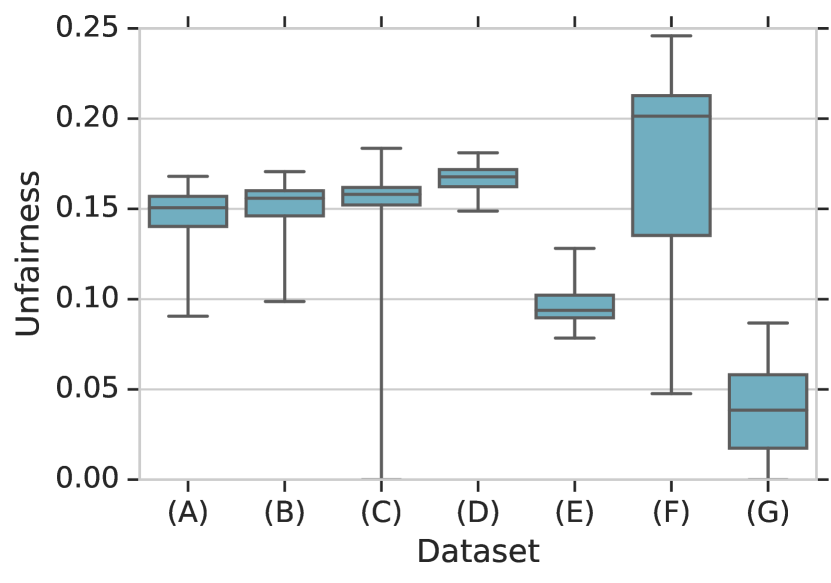
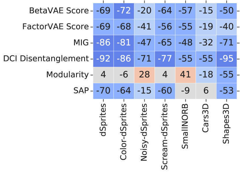
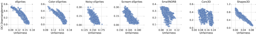
Figure 2: (Left) Distribution of unfairness for learned representations. Legend: dSprites = (A), Color-dSprites = (B), Noisy-dSprites = (C), Scream-dSprites = (D), SmallNORB = (E), Cars3D = (F), Shapes3D = (G). (Right) Rank correlation of unfairness and disentanglement scores on the various data sets.

Figure 3: Unfairness of representations versus DCI Disentanglement on the different data sets.

4.1 The unfairness of general purpose representations and the relation to dientanglement

In Figure 3 (left), we show the distribution of unfairness scores for different representations on different data sets. We clearly observe that learned representations can be unfair, even in the setting where the target variable and the sensitive variable are independent. In particular, the total variation can reach as much as $15\%-25\%$ on five out of seven data sets. This confirms the importance of trying to find general-purpose representations that are less unfair.

We also observe in Figure 3 (left) that there is considerable spread in unfairness scores for different learned representations. This indicates that the specific representation used matters and that predictions with low unfairness can be achieved. To investigate whether disentanglement is a useful property to guarantee less unfair representations, we show rank correlation between a wide range of disentanglement scores and the unfairness score in Figure 3 (right). We observe that all disentanglement scores except Modularity appear to be consistently correlated with a lower unfairness score for all data sets. While the considered disentanglement metrics (except Modularity) have been found to be correlated (see [61]), we observe significant differences in between scores: Figure 3 (right) indicates that DCI Disentanglement is correlated the most followed by the Mutual Information Gap, the BetaVAE score, the FactorVAE score, the SAP score and finally Modularity. The strong correlation of DCI Disentanglement is confirmed by Figure 3 where we plot the Unfairness score against the DCI Disentanglement score for each model. Again, we observe that the large gap in unfairness seem to be related to differences in the representation. We show the corresponding plots for all metrics in Figure 9 in the Appendix.

These results provide an encouraging case for disentanglement being helpful in finding fairer representations. However, they should be interpreted with care: Even though we have considered a diverse set of methods and disentangled representations, the computed correlation scores depend on the distribution of considered models. If one were to consider an entirely different set of methods, hyperparameters and corresponding representations, the observed relationship may differ.

4.2 Adjusting for downstream performance

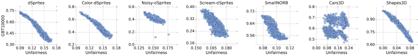
Figure 4: Unfairness of representations versus downstream accuracy on the different data sets.

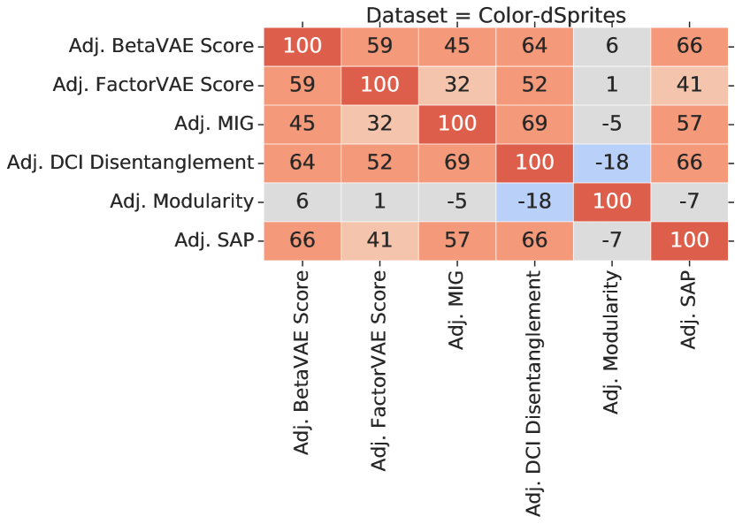
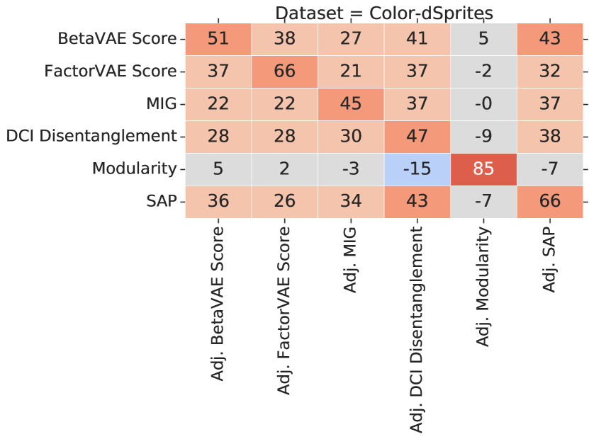
Figure 5: Rank correlation between the adjusted disentanglement scores (left) and between original scores and the adjusted version (right).

Prior work [61] has observed that disentanglement metrics are correlated with how well ground-truth factors of variations can be predicted from the representation using gradient boosted trees. It is thus not surprising that the unfairness of a representation is also consistently correlated to the average accuracy of a gradient boosted trees classifier using $10\,000$ samples (see Figure 5). In this section, we investigate whether disentanglement is also correlated with a higher fairness if we compare representations with the same accuracy as measured by GBT10000 scores. Given two representations with the same downstream performance, is the more disentangled one also more fair? The key challenge is that for a given representation there may not be other ones with exactly the same downstream performance.

For this, we adjust all the disentanglement scores and the unfairness score for the effect of downstream performance. We use a k-nearest neighbors regression from Scikit-learn [72] to predict, for any model, each disentanglement score and the unfairness from its five nearest neighbor in terms of GBT10000 (which we write as $N(\text{GBT10000})$). This can be seen as a one-dimensional non-parametric estimate of the disentanglement score (or fairness score) based on the GBT10000 score. The adjusted metric is computed as the residual score after the average score of the neighbors is subtracted, namely

$$\texttt{Adj. Metric}=\texttt{Metric}-\frac{1}{5}\sum_{i\in N(\text{GBT10000})}\texttt{Metric}_{i}$$

Intuitively, the adjusted metrics measure how much more disentangled (fairer) a given representation is compared to an average representation with the same downstream performance.

In Figure 5 (left), we observe that the rank correlation between the adjusted disentanglement scores (except Modularity) on Color-dSprites is consistenly positive. This indicates that the adjusted scores do measure a similar property of the representation even when adjusted for performance. This result is consistent across data sets (Figure 11 of the Appendix). The only exception appears to be SmallNORB, where the adjusted DCI Disentanglement, MIG and SAP score correlate with each other but do not correlate well with the BetaVAE and FactorVAE score (which only correlate with each other). On Shapes3D we observe a similar result, but the correlation between the two groups of scores is stronger than on SmallNORB. Similarly, Figure 5 (right) shows the rank correlation between the disentanglement metrics and their adjusted versions. As expected, we observe that there still is a significant positive correlation. This indicates the adjusted scores still capture a significant part of the unadjusted score. We observe in Figure 11 of the Appendix that this result appears to be consistent across the different data sets, again with the exception of SmallNORB. As a sanity check, we finally confirm by visual inspection that the adjusted metrics still measure disentanglement. In Figure 6, we plot latent traversals for the model with highest adjusted MIG score on Shapes3D and observe that the model appears well disentangled.

Figure 6: Latent traversals (each column corresponds to a different latent variable being varied) on Shapes3D for the model with best adjusted MIG.

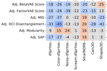
Figure 7: Rank correlation of unfairness and disentanglement scores on the various data sets (left). Rank correlation of adjusted unfairness and adjusted disentanglement scores on the various data sets (right).

Finally, Figure 7 shows the rank correlation between the adjusted disentanglement scores and the adjusted fairness score for each of the data sets. Overall, we observe that higher disentanglement still seems to be correlated with an increased fairness, even when accounting for downstream performance. Exceptions appear to be the adjusted Modularity score, the adjusted BetaVAE and the FactorVAE score on Shapes3D, and the adjusted MIG, DCI Disentanglement, Modularity and SAP on SmallNORB. As expected, the correlations appear to be weaker than for the unadjusted scores (see Figure 3 (right)) but we still observe some residual correlation.

How do we identify fair models?

In this section, we observed that disentangled representations allow to train fairer classifiers, regardless of their accuracy. This leaves us with the question of how can we find fair representations? [61] showed that without access to supervision or inductive biases, disentangled representations cannot be identified. However, existing methods heavily rely on inductive biases such as architecture, hyperparameter choices, mean-field assumptions, and smoothness induced through randomness [65, 80, 86]. In practice, training a large number of models with different losses and hyperparameters will result in a large number of different representations, some of which might be more disentangled than others as can be seen for example in Figure 3. From Theorem 1, we know that optimizing for accuracy on a fixed representation does not guarantee to learn a fair classifier as the demographic parity theoretically depends on the representation when the sensitive variable is not observed.

When we fix a classification algorithm, in our case GBT10000, and we train it over a variety of representations with different degrees of disentanglement we obtain both different degrees of fairness and downstream performance. If the disentanglement of the representation is the only confounder between the performance of the classifier and its fairness as depicted in Figure 8, the classification accuracy may be used as a proxy for fairness. To test whether this holds in practice, we perform the following experiment. We sample a data set, a seed for the unsupervised disentanglement models and among the factors of variations we sample one to be ${\mathbf{y}}$ and one to be ${\mathbf{s}}$. Then, we train a classifier predicting ${\mathbf{y}}$ from $r({\mathbf{x}})$ using all the models trained on that data set on the specific seed. We compare the unfairness of the classifier achieving highest prediction accuracy on ${\mathbf{y}}$ with a randomly chosen classifier from the ones we trained. We observe that the classifier selected using test accuracy is also fairer 84.2% of the times. We remark that this result explicitly make use of a large amount of representations of different quality on which we train the same classification algorithm. Under the assumption of Figure 8, the disentanglement of the representation is the only difference explaining different predictions, the best performing classifier is also more fair than one trained on a different representation. Since disentanglement is likely not the only confounder, model selection based on downstream performance is not guaranteed to always be fairer than random model selection.

5 Related Work

Figure 8: If disentanglement is a causal parent of downstream performance and fairness and there are no hidden confounders, then the former can be used as a proxy for the latter.

Ideas related to disentangling the factors of variations have a long tradition in machine learning, dating back to the non-linear ICA literature [17, 3, 46, 42, 43, 44, 32]. Disentangling pose from content and content from motion are also classical computer vision problems that have been tackled with various degrees of supervision and inductive bias [92, 93, 40, 25, 18, 31, 42]. In this paper, we intend disentanglement in the sense of [6, 87, 35, 61]. [61] recently proved that without access to supervision or inductive biases, disentanglement learning is impossible as disentangled models cannot be identified. In this paper, we evaluate the representation using the supervised downstream task where both target and sensitive variables are observed. Semi-supervised variants have been extensively studied during the years. [77, 15, 66, 70, 50, 52, 1] assume partially observed factors of variation that should be disentangled from the other unobserved ones. Weaker forms of supervision like relational information or additional assumptions on the effect of the factors of variation were also studied [39, 16, 47, 31, 91, 26, 19, 41, 93, 62, 53, 81, 8] and applied in the sequential data and reinforcement learning settings [88, 85, 57, 69, 37, 38]. Overall, the disentanglement literature is interested in isolating the effect of every factor of variation regardless of how the representation should be used downstream.

On the fairness perspective, representation learning has been used as a mean to separate the detrimental effects that labeled sensitive factors could have on the classification task [67, 34]. We remark that this setup is different from what we consider in this paper, as we do not assume access to any labeled information when learning a representation. In particular, we do not assume to know what the downstream task will be and what are the sensible variables (if any). [21, 95] introduce the idea that a fair representation should preserve all information about the individual’s attributes except for the membership to protected groups. In practice, [63] extends the VAE objective with a Maximum Mean Discrepancy [33] to ensure independence between the latent representation and the sensitive factors. [12] introduces the idea of data pre-processing as a tool to control for downstream discrimination. The authors of [84] instead propose an information-theoretic approach in which the mutual information between the data and the representation is maximized, while the one between the sensitive attributes and the representation is minimized. Furthermore, there are several approaches that employ adversarial [30] training to avoid information leakage between the sensitive attributes and the representation [23, 64, 96]. Finally, representation learning has recently proved to be useful in counterfactual fairness [55, 45].

6 Conclusion

In this paper, we observe the first empirical evidence that disentanglement might prove beneficial to learn fair representations, providing evidence supporting the conjectures of [61, 54]. We show that general purpose representations can lead to substantial unfairness, even in the setting where both the sensitive variable and target variable are independent and one only has access to observations that depend on both of them. Yet, the choice of representation appears to be crucial as we find that that increased disentanglement of a representation is consistently correlated with increased fairness on downstream prediction tasks across a wide range of representations and data sets. Furthermore, we discuss the relationship between fairness, downstream accuracy and disentanglement and find evidence that the correlation between disentanglement metrics and the unfairness of the downstream prediction tasks appears to also hold if one accounts for the downstream accuracy. We believe that these results serve as a motivation for further investigation on the practical benefits of disentangled representations, especially in the context of fairness. Finally, we argue that fairness should be among the desired properties of general purpose representation learning beyond VAEs [20, 76]. As we highlighted in this paper, it appears possible to learn representations that are both useful, interpretable and fairer. Progress on this problem could allow machine-learning driven decision making to be both better and fairer.

Appendix A Proof of Theorem 1

See 1

Proof.

Our proof is by counter example. We present a simple case for which ${\mathbf{y}}$ is predicted from ${\mathbf{x}}$ in such a way that $p(\hat{\mathbf{y}}|{\mathbf{x}})=p({\mathbf{y}}|{\mathbf{x}})$, but which does not satisfy demographic parity.

We assume all variables to be Bernoulli-distributed $p({\mathbf{s}}=1)=q,\,0<q<1$ and $p({\mathbf{y}}=1)=b,\,0<b<1$ and our mixing mechanism to be ${\mathbf{x}}=\min({\mathbf{y}},{\mathbf{s}})$. The assumption of demographic parity yields:

$$DP \implies p(\hat{\mathbf{y}}=1|{\mathbf{s}}=1)=p(\hat{\mathbf{y}}=1|{\mathbf{s}}=0)$$

$$\implies\sum_{{\mathbf{x}}\in\{0,1\}}p(\hat{\mathbf{y}}=1,{\mathbf{x}}|{\mathbf{s}}=1)=\sum_{{\mathbf{x}}\in\{0,1\}}p(\hat{\mathbf{y}}=1,{\mathbf{x}}|{\mathbf{s}}=0)$$

where the first implication comes from the definition of demographic parity. Using the causal Markov condition [74], we can rewrite $p(\hat{\mathbf{y}}=1,{\mathbf{x}}|{\mathbf{s}})=p(\hat{\mathbf{y}}=1|{\mathbf{x}})p({\mathbf{x}}|{\mathbf{s}})$ and thus

$$DP \implies\sum_{{\mathbf{x}}\in\{0,1\}}p(\hat{\mathbf{y}}=1|{\mathbf{x}})p({\mathbf{x}}|{\mathbf{s}}=1)=\sum_{{\mathbf{x}}\in\{0,1\}}p(\hat{\mathbf{y}}=1|{\mathbf{x}})p({\mathbf{x}}|{\mathbf{s}}=0)$$

The rest of the proof follows as a proof by contradiction. Assuming that the classifier is perfect, i.e., $p(\hat{\mathbf{y}}|{\mathbf{x}})=p({\mathbf{y}}|{\mathbf{x}})$, we have

$$DP \implies\sum_{{\mathbf{x}}\in\{0,1\}}p({\mathbf{y}}=1|{\mathbf{x}})p({\mathbf{x}}|{\mathbf{s}}=1)=\sum_{{\mathbf{x}}\in\{0,1\}}p({\mathbf{y}}=1|{\mathbf{x}})p({\mathbf{x}}|{\mathbf{s}}=0)$$

$$\implies\sum_{{\mathbf{x}}\in\{0,1\}}p({\mathbf{y}}=1|{\mathbf{x}})\left[p({\mathbf{x}}|{\mathbf{s}}=1)-p({\mathbf{x}}|{\mathbf{s}}=0)\right]=0$$

$$\implies p({\mathbf{y}}=1|{\mathbf{x}}=0)\left[p({\mathbf{x}}=0|{\mathbf{s}}=1)-p({\mathbf{x}}=0|{\mathbf{s}}=0)\right]+$$

$$\qquad\qquad p({\mathbf{y}}=1|{\mathbf{x}}=1)\left[p({\mathbf{x}}=1|{\mathbf{s}}=1)-p({\mathbf{x}}=1|{\mathbf{s}}=0)\right]=0.$$

At this point, using the fact that $${\mathbf{x}}=\min({\mathbf{y}},{\mathbf{s}}) p({\mathbf{x}}=0|{\mathbf{s}}=1)=p({\mathbf{y}}=0) p({\mathbf{x}}=0|{\mathbf{s}}=0)=1 p({\mathbf{y}}=1|{\mathbf{x}}=1)=1 p({\mathbf{x}}=1|{\mathbf{s}}=1)=p({\mathbf{y}}=1) p({\mathbf{x}}=1|{\mathbf{s}}=0)=0$$, we have ,  ,  ,  ,  and  , therefore

$$DP \implies p({\mathbf{y}}=1|{\mathbf{x}}=0)\left[p({\mathbf{y}}=0)-1\right]+1\cdot\left[p({\mathbf{y}}=1)-0\right]=0$$

$$\implies-b\cdot p({\mathbf{y}}=1|{\mathbf{x}}=0)+b=0$$

$$\implies p({\mathbf{y}}=1|{\mathbf{x}}=0)=1$$

$$\implies p({\mathbf{x}}=0|{\mathbf{y}}=1)p({\mathbf{y}}=1)=p({\mathbf{x}}=0)$$

$$\implies p({\mathbf{s}}=0)p({\mathbf{y}}=1)=p({\mathbf{x}}=0)$$

$$\implies(1-q)b=(1-q)+q(1-b)$$

$$\implies 0=(1-q)(1-b)+q(1-b)$$

$$\implies b=1$$

Hence we have our desired contradiction as, by assumption, $b<1$. ∎

Appendix B Additional Results

In Figure 9, we plot the unfairness of the classifier against the disentanglement of the representation measured with all the different disentanglement metrics. We observe that unfairness and disentanglement appear to be generally correlated with the exception of Modularity and, partially, of the SAP score. This plot extends Figure 3 to all disentanglement scores.

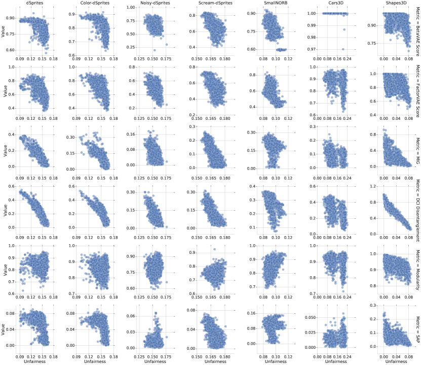
Figure 9: Unfairness of representations versus disentanglement scores on the different data sets.

In Figure 11, we plot the rank correlation between the adjusted metrics. We observe a similar correlation to the one observed in [61] with the non-adjusted metrics. In Figure 11, we plot the rank correlation between adjusted and non-adjusted metrics. These plots extend Figure 5 to all data sets. We conclude that the correlation between the disentanglement metrics is not exclusively driven by the downstream performance and the adjusted metrics are suitable to discuss the fairness of the representation independently from the classification accuracy of the downstream classifier.

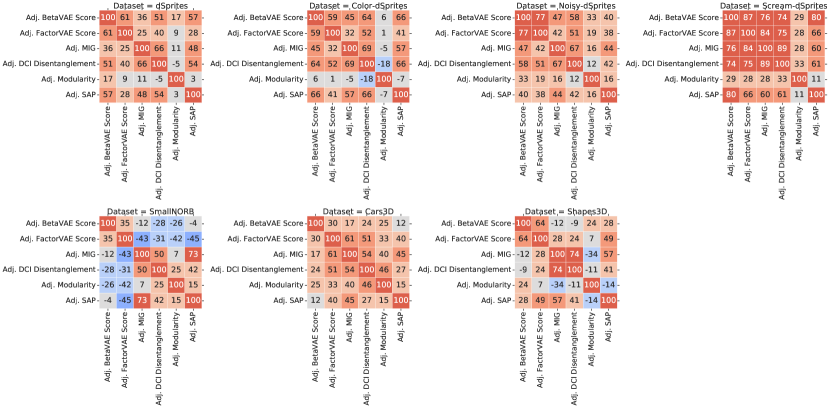
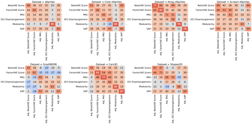
Figure 10: Rank correlation between the adjusted disentanglement scores.

Figure 11: Rank correlation between disentanglement scores and the adjusted version.

References

- [1] Tameem Adel, Zoubin Ghahramani, and Adrian Weller. Discovering interpretable representations for both deep generative and discriminative models. In International Conference on Machine Learning, pages 50–59, 2018.
- [2] Alexander A Alemi, Ian Fischer, Joshua V Dillon, and Kevin Murphy. Deep variational information bottleneck. arXiv preprint arXiv:1612.00410, 2016.
- [3] Francis Bach and Michael Jordan. Kernel independent component analysis. Journal of Machine Learning Research, 3(7):1–48, 2002.
- [4] Solon Barocas, Moritz Hardt, and Arvind Narayanan. Fairness and machine learning. https://fairmlbook.org/, 2019.
- [5] Solon Barocas and Andrew D Selbst. Big data’s disparate impact. Calif. L. Rev., 104:671, 2016.
- [6] Yoshua Bengio, Aaron Courville, and Pascal Vincent. Representation learning: A review and new perspectives. IEEE Transactions on Pattern Analysis and Machine Intelligence, 35(8):1798–1828, 2013.
- [7] Yoshua Bengio, Yann LeCun, et al. Scaling learning algorithms towards AI. Large-scale Kernel Machines, 34(5):1–41, 2007.
- [8] Diane Bouchacourt, Ryota Tomioka, and Sebastian Nowozin. Multi-level variational autoencoder: Learning disentangled representations from grouped observations. In AAAI Conference on Artificial Intelligence, 2018.
- [9] Christopher P Burgess, Irina Higgins, Arka Pal, Loic Matthey, Nick Watters, Guillaume Desjardins, and Alexander Lerchner. Understanding disentangling in beta-VAE. arXiv preprint arXiv:1804.03599, 2018.
- [10] Toon Calders, Faisal Kamiran, and Mykola Pechenizkiy. Building classifiers with independency constraints. In 2009 IEEE International Conference on Data Mining Workshops, pages 13–18. IEEE, 2009.
- [11] Toon Calders and Indrė Žliobaitė. Why unbiased computational processes can lead to discriminative decision procedures. In Discrimination and privacy in the information society, pages 43–57. Springer, 2013.
- [12] Flavio Calmon, Dennis Wei, Bhanukiran Vinzamuri, Karthikeyan Natesan Ramamurthy, and Kush R Varshney. Optimized pre-processing for discrimination prevention. In Advances in Neural Information Processing Systems, pages 3992–4001, 2017.
- [13] Tian Qi Chen, Xuechen Li, Roger Grosse, and David Duvenaud. Isolating sources of disentanglement in variational autoencoders. In Advances in Neural Information Processing Systems, 2018.
- [14] Xi Chen, Yan Duan, Rein Houthooft, John Schulman, Ilya Sutskever, and Pieter Abbeel. Infogan: Interpretable representation learning by information maximizing generative adversarial nets. In Advances in Neural Information Processing Systems, 2016.
- [15] Brian Cheung, Jesse A Livezey, Arjun K Bansal, and Bruno A Olshausen. Discovering hidden factors of variation in deep networks. arXiv preprint arXiv:1412.6583, 2014.
- [16] Taco Cohen and Max Welling. Learning the irreducible representations of commutative lie groups. In International Conference on Machine Learning, 2014.
- [17] Pierre Comon. Independent component analysis, a new concept? Signal Processing, 36(3):287–314, 1994.
- [18] Zhiwei Deng, Rajitha Navarathna, Peter Carr, Stephan Mandt, Yisong Yue, Iain Matthews, and Greg Mori. Factorized variational autoencoders for modeling audience reactions to movies. In IEEE Conference on Computer Vision and Pattern Recognition, 2017.
- [19] Emily L Denton and Vighnesh Birodkar. Unsupervised learning of disentangled representations from video. In Advances in Neural Information Processing Systems, 2017.
- [20] Vincent Dumoulin, Ishmael Belghazi, Ben Poole, Olivier Mastropietro, Alex Lamb, Martin Arjovsky, and Aaron Courville. Adversarially learned inference. In International Conference on Learning Representations, 2016.
- [21] Cynthia Dwork, Moritz Hardt, Toniann Pitassi, Omer Reingold, and Richard Zemel. Fairness through awareness. In Proceedings of the 3rd innovations in theoretical computer science conference, pages 214–226. ACM, 2012.
- [22] Cian Eastwood and Christopher KI Williams. A framework for the quantitative evaluation of disentangled representations. In International Conference on Learning Representations, 2018.
- [23] Harrison Edwards and Amos Storkey. Censoring representations with an adversary. arXiv preprint arXiv:1511.05897, 2015.
- [24] Babak Esmaeili, Hao Wu, Sarthak Jain, Alican Bozkurt, N Siddharth, Brooks Paige, Dana H Brooks, Jennifer Dy, and Jan-Willem Meent. Structured disentangled representations. In The 22nd International Conference on Artificial Intelligence and Statistics, pages 2525–2534, 2019.
- [25] Vincent Fortuin, Matthias Hüser, Francesco Locatello, Heiko Strathmann, and Gunnar Rätsch. Deep self-organization: Interpretable discrete representation learning on time series. In International Conference on Learning Representations, 2019.
- [26] Marco Fraccaro, Simon Kamronn, Ulrich Paquet, and Ole Winther. A disentangled recognition and nonlinear dynamics model for unsupervised learning. In Advances in Neural Information Processing Systems, 2017.
- [27] Jerome H Friedman. Greedy function approximation: a gradient boosting machine. Annals of statistics, pages 1189–1232, 2001.
- [28] Muhammad Waleed Gondal, Manuel Wüthrich, Djordje Miladinović, Francesco Locatello, Martin Breidt, Valentin Volchkov, Joel Akpo, Olivier Bachem, Bernhard Schölkopf, and Stefan Bauer. On the transfer of inductive bias from simulation to the real world: a new disentanglement dataset. In Advances in Neural Information Processing Systems, 2019.
- [29] Ian Goodfellow, Honglak Lee, Quoc V Le, Andrew Saxe, and Andrew Y Ng. Measuring invariances in deep networks. In Advances in Neural Information Processing Systems, 2009.
- [30] Ian Goodfellow, Jean Pouget-Abadie, Mehdi Mirza, Bing Xu, David Warde-Farley, Sherjil Ozair, Aaron Courville, and Yoshua Bengio. Generative adversarial nets. In Advances in neural information processing systems, pages 2672–2680, 2014.
- [31] Ross Goroshin, Michael F Mathieu, and Yann LeCun. Learning to linearize under uncertainty. In Advances in Neural Information Processing Systems, 2015.
- [32] Luigi Gresele, Paul K. Rubenstein, Arash Mehrjou, Francesco Locatello, and Bernhard Schölkopf. The incomplete rosetta stone problem: Identifiability results for multi-view nonlinear ica. In Conference on Uncertainty in Artificial Intelligence (UAI), 2019.
- [33] Arthur Gretton, Karsten Borgwardt, Malte Rasch, Bernhard Schölkopf, and Alex J Smola. A kernel method for the two-sample-problem. In Advances in neural information processing systems, pages 513–520, 2007.
- [34] Moritz Hardt, Eric Price, Nati Srebro, et al. Equality of opportunity in supervised learning. In Advances in neural information processing systems, pages 3315–3323, 2016.
- [35] Irina Higgins, David Amos, David Pfau, Sebastien Racaniere, Loic Matthey, Danilo Rezende, and Alexander Lerchner. Towards a definition of disentangled representations. arXiv preprint arXiv:1812.02230, 2018.
- [36] Irina Higgins, Loic Matthey, Arka Pal, Christopher Burgess, Xavier Glorot, Matthew Botvinick, Shakir Mohamed, and Alexander Lerchner. beta-VAE: Learning basic visual concepts with a constrained variational framework. In International Conference on Learning Representations, 2017.
- [37] Irina Higgins, Arka Pal, Andrei Rusu, Loic Matthey, Christopher Burgess, Alexander Pritzel, Matthew Botvinick, Charles Blundell, and Alexander Lerchner. Darla: Improving zero-shot transfer in reinforcement learning. In International Conference on Machine Learning, 2017.
- [38] Irina Higgins, Nicolas Sonnerat, Loic Matthey, Arka Pal, Christopher P Burgess, Matko Bošnjak, Murray Shanahan, Matthew Botvinick, Demis Hassabis, and Alexander Lerchner. Scan: Learning hierarchical compositional visual concepts. In International Conference on Learning Representations, 2018.
- [39] Geoffrey E Hinton, Alex Krizhevsky, and Sida D Wang. Transforming auto-encoders. In International Conference on Artificial Neural Networks, 2011.
- [40] Jun-Ting Hsieh, Bingbin Liu, De-An Huang, Li F Fei-Fei, and Juan Carlos Niebles. Learning to decompose and disentangle representations for video prediction. In Advances in Neural Information Processing Systems, 2018.
- [41] Wei-Ning Hsu, Yu Zhang, and James Glass. Unsupervised learning of disentangled and interpretable representations from sequential data. In Advances in Neural Information Processing Systems, 2017.
- [42] Aapo Hyvarinen and Hiroshi Morioka. Unsupervised feature extraction by time-contrastive learning and nonlinear ica. In Advances in Neural Information Processing Systems, 2016.
- [43] Aapo Hyvärinen and Petteri Pajunen. Nonlinear independent component analysis: Existence and uniqueness results. Neural Networks, 1999.
- [44] Aapo Hyvarinen, Hiroaki Sasaki, and Richard E Turner. Nonlinear ica using auxiliary variables and generalized contrastive learning. In International Conference on Artificial Intelligence and Statistics, 2019.
- [45] Fredrik Johansson, Uri Shalit, and David Sontag. Learning representations for counterfactual inference. In International conference on machine learning, pages 3020–3029, 2016.
- [46] Christian Jutten and Juha Karhunen. Advances in nonlinear blind source separation. In International Symposium on Independent Component Analysis and Blind Signal Separation, pages 245–256, 2003.
- [47] Theofanis Karaletsos, Serge Belongie, and Gunnar Rätsch. Bayesian representation learning with oracle constraints. arXiv preprint arXiv:1506.05011, 2015.
- [48] N. Kilbertus, M. Rojas Carulla, G. Parascandolo, M. Hardt, D. Janzing, and B. Schölkopf. Avoiding discrimination through causal reasoning. In Advances in Neural Information Processing Systems 30, pages 656–666, 2017.
- [49] Hyunjik Kim and Andriy Mnih. Disentangling by factorising. In International Conference on Machine Learning, 2018.
- [50] Diederik P Kingma, Shakir Mohamed, Danilo Jimenez Rezende, and Max Welling. Semi-supervised learning with deep generative models. In Advances in Neural Information Processing Systems, 2014.
- [51] Diederik P Kingma and Max Welling. Auto-encoding variational Bayes. In International Conference on Learning Representations, 2014.
- [52] Jack Klys, Jake Snell, and Richard Zemel. Learning latent subspaces in variational autoencoders. In Advances in Neural Information Processing Systems, 2018.
- [53] Tejas D Kulkarni, William F Whitney, Pushmeet Kohli, and Josh Tenenbaum. Deep convolutional inverse graphics network. In Advances in Neural Information Processing Systems, 2015.
- [54] Abhishek Kumar, Prasanna Sattigeri, and Avinash Balakrishnan. Variational inference of disentangled latent concepts from unlabeled observations. In International Conference on Learning Representations, 2018.
- [55] Matt J Kusner, Joshua Loftus, Chris Russell, and Ricardo Silva. Counterfactual fairness. In Advances in Neural Information Processing Systems, pages 4066–4076, 2017.
- [56] Brenden M Lake, Tomer D Ullman, Joshua B Tenenbaum, and Samuel J Gershman. Building machines that learn and think like people. Behavioral and Brain Sciences, 40, 2017.
- [57] Adrien Laversanne-Finot, Alexandre Pere, and Pierre-Yves Oudeyer. Curiosity driven exploration of learned disentangled goal spaces. In Conference on Robot Learning, 2018.
- [58] Yann LeCun, Yoshua Bengio, and Geoffrey Hinton. Deep learning. Nature, 521(7553):436, 2015.
- [59] Yann LeCun, Fu Jie Huang, and Leon Bottou. Learning methods for generic object recognition with invariance to pose and lighting. In IEEE Conference on Computer Vision and Pattern Recognition, 2004.
- [60] Karel Lenc and Andrea Vedaldi. Understanding image representations by measuring their equivariance and equivalence. In IEEE Conference on Computer Vision and Pattern Recognition, 2015.
- [61] Francesco Locatello, Stefan Bauer, Mario Lucic, Sylvain Gelly, Bernhard Schölkopf, and Olivier Bachem. Challenging common assumptions in the unsupervised learning of disentangled representations. In (To appear) International Conference on Machine Learning, 2019.
- [62] Francesco Locatello, Damien Vincent, Ilya Tolstikhin, Gunnar Rätsch, Sylvain Gelly, and Bernhard Schölkopf. Competitive training of mixtures of independent deep generative models. In Workshop at the 6th International Conference on Learning Representations (ICLR), 2018.
- [63] Christos Louizos, Kevin Swersky, Yujia Li, Max Welling, and Richard Zemel. The variational fair autoencoder. arXiv preprint arXiv:1511.00830, 2015.
- [64] David Madras, Elliot Creager, Toniann Pitassi, and Richard Zemel. Learning adversarially fair and transferable representations. arXiv preprint arXiv:1802.06309, 2018.
- [65] Emile Mathieu, Tom Rainforth, N. Siddharth, and Yee Whye Teh. Disentangling disentanglement in variational auto-encoders. arXiv preprint arXiv:1812.02833, 2018.
- [66] Michael F Mathieu, Junbo J Zhao, Aditya Ramesh, Pablo Sprechmann, and Yann LeCun. Disentangling factors of variation in deep representation using adversarial training. In Advances in Neural Information Processing Systems, 2016.
- [67] Daniel McNamara, Cheng Soon Ong, and Robert C Williamson. Provably fair representations. arXiv preprint arXiv:1710.04394, 2017.
- [68] C Munoz, M Smith, and DJ Patil. Big data: A report on algorithmic systems, opportunity, and civil rights. executive office of the president, may, 2016.
- [69] Ashvin V Nair, Vitchyr Pong, Murtaza Dalal, Shikhar Bahl, Steven Lin, and Sergey Levine. Visual reinforcement learning with imagined goals. In Advances in Neural Information Processing Systems, 2018.
- [70] Siddharth Narayanaswamy, T Brooks Paige, Jan-Willem Van de Meent, Alban Desmaison, Noah Goodman, Pushmeet Kohli, Frank Wood, and Philip Torr. Learning disentangled representations with semi-supervised deep generative models. In Advances in Neural Information Processing Systems, 2017.
- [71] Judea Pearl. Causality. Cambridge University Press, 2009.
- [72] F. Pedregosa, G. Varoquaux, A. Gramfort, V. Michel, B. Thirion, O. Grisel, M. Blondel, P. Prettenhofer, R. Weiss, V. Dubourg, J. Vanderplas, A. Passos, D. Cournapeau, M. Brucher, M. Perrot, and E. Duchesnay. Scikit-learn: Machine learning in Python. Journal of Machine Learning Research, 12:2825–2830, 2011.
- [73] Dino Pedreshi, Salvatore Ruggieri, and Franco Turini. Discrimination-aware data mining. In Proceedings of the 14th ACM SIGKDD international conference on Knowledge discovery and data mining, pages 560–568. ACM, 2008.
- [74] Jonas Peters, Dominik Janzing, and Bernhard Schölkopf. Elements of Causal Inference - Foundations and Learning Algorithms. Adaptive Computation and Machine Learning Series. MIT Press, 2017.
- [75] John Podesta, Penny Pritzker, Ernest J Moniz, John Holdren, and Jeffrey Zients. Big data: Seizing opportunities, preserving values. executive office of the president. washington, dc: The white house, 2014.
- [76] Ben Poole, Sherjil Ozair, Aaron van den Oord, Alexander A Alemi, and George Tucker. On variational bounds of mutual information. In International Conference on Machine Learning, pages 5171–5180, 2019.
- [77] Scott Reed, Kihyuk Sohn, Yuting Zhang, and Honglak Lee. Learning to disentangle factors of variation with manifold interaction. In International Conference on Machine Learning, 2014.
- [78] Scott Reed, Yi Zhang, Yuting Zhang, and Honglak Lee. Deep visual analogy-making. In Advances in Neural Information Processing Systems, 2015.
- [79] Karl Ridgeway and Michael C Mozer. Learning deep disentangled embeddings with the f-statistic loss. In Advances in Neural Information Processing Systems, 2018.
- [80] Michal Rolinek, Dominik Zietlow, and Georg Martius. Variational autoencoders recover pca directions (by accident). In Proceedings IEEE Conf. on Computer Vision and Pattern Recognition, 2019.
- [81] Adrià Ruiz, Oriol Martinez, Xavier Binefa, and Jakob Verbeek. Learning disentangled representations with reference-based variational autoencoders. arXiv preprint arXiv:1901.08534, 2019.
- [82] Jürgen Schmidhuber. Learning factorial codes by predictability minimization. Neural Computation, 4(6):863–879, 1992.
- [83] Wim Schreurs, Mireille Hildebrandt, Els Kindt, and Michaël Vanfleteren. Cogitas, ergo sum. the role of data protection law and non-discrimination law in group profiling in the private sector. In Profiling the European citizen, pages 241–270. Springer, 2008.
- [84] Jiaming Song, Pratyusha Kalluri, Aditya Grover, Shengjia Zhao, and Stefano Ermon. Learning controllable fair representations. arXiv preprint arXiv:1812.04218, 2018.
- [85] Xander Steenbrugge, Sam Leroux, Tim Verbelen, and Bart Dhoedt. Improving generalization for abstract reasoning tasks using disentangled feature representations. In Workshop on Relational Representation Learning at NeurIPS, 2018.
- [86] Jan Stühmer, Richard Turner, and Sebastian Nowozin. ISA-VAE: Independent subspace analysis with variational autoencoders, 2019.
- [87] Raphael Suter, Djordje Miladinović, Stefan Bauer, and Bernhard Schölkopf. Interventional robustness of deep latent variable models. In (To appear) International Conference on Machine Learning, 2019.
- [88] Valentin Thomas, Emmanuel Bengio, William Fedus, Jules Pondard, Philippe Beaudoin, Hugo Larochelle, Joelle Pineau, Doina Precup, and Yoshua Bengio. Disentangling the independently controllable factors of variation by interacting with the world. Learning Disentangled Representations Workshop at NeurIPS, 2017.
- [89] Michael Tschannen, Olivier Bachem, and Mario Lucic. Recent advances in autoencoder-based representation learning. arXiv preprint arXiv:1812.05069, 2018.
- [90] Sjoerd van Steenkiste, Francesco Locatello, Jürgen Schmidhuber, and Olivier Bachem. Are disentangled representations helpful for abstract visual reasoning? arXiv preprint arXiv:1905.12506, 2019.
- [91] William F Whitney, Michael Chang, Tejas Kulkarni, and Joshua B Tenenbaum. Understanding visual concepts with continuation learning. arXiv preprint arXiv:1602.06822, 2016.
- [92] Jimei Yang, Scott E Reed, Ming-Hsuan Yang, and Honglak Lee. Weakly-supervised disentangling with recurrent transformations for 3D view synthesis. In Advances in Neural Information Processing Systems, 2015.
- [93] Li Yingzhen and Stephan Mandt. Disentangled sequential autoencoder. In International Conference on Machine Learning, 2018.
- [94] Muhammad Bilal Zafar, Isabel Valera, Manuel Gomez Rodriguez, and Krishna P Gummadi. Fairness beyond disparate treatment & disparate impact: Learning classification without disparate mistreatment. In Proceedings of the 26th International Conference on World Wide Web, pages 1171–1180. International World Wide Web Conferences Steering Committee, 2017.
- [95] Rich Zemel, Yu Wu, Kevin Swersky, Toni Pitassi, and Cynthia Dwork. Learning fair representations. In International Conference on Machine Learning, pages 325–333, 2013.
- [96] Brian Hu Zhang, Blake Lemoine, and Margaret Mitchell. Mitigating unwanted biases with adversarial learning. In Proceedings of the 2018 AAAI/ACM Conference on AI, Ethics, and Society, pages 335–340. ACM, 2018.
- [97] Indre Zliobaite. On the relation between accuracy and fairness in binary classification. arXiv preprint arXiv:1505.05723, 2015.