On Policy Evaluation with Aggregate Time-Series Shocks

Abstract

We propose a new estimator for causal effects in applications where the exogenous variation comes from aggregate time-series shocks. We address the critical identification challenge in such applications – unobserved confounding, which renders conventional estimators invalid. Our estimator uses a new data-based aggregation scheme and remains consistent in the presence of unobserved aggregate shocks. We illustrate the advantages of our algorithm using data from Nakamura and Steinsson (2014). We also establish the statistical properties of our estimator in a practically relevant regime, where both cross-sectional and time-series dimensions are large, and show how to use our method to conduct inference.

Keywords: Continuous Difference in Differences, Panel Data, Causal Effects, Instrumental Variables, Treatment Effects, Unobserved Heterogeneity, Synthetic Control.

JEL Classification: C18, C21, C23, C26.

1 Introduction

Changes in aggregate variables are commonly used to evaluate economic policies. The most popular design of this type is an “event study”, where a one-time aggregate shock, e.g., a new law, affects some units but not others, and we observe both groups over time. To quantify the effect of this shock, practitioners use either difference in differences or, more recently, synthetic control methodology (e.g., Ashenfelter and Card, 1985; Card and Krueger, 1994; Abadie and Gardeazabal, 2003; Bertrand et al., 2004; Abadie et al., 2010). Often, when both outcome and treatment variables vary at the unit level, this approach is used as a first stage, and the aggregate change effectively plays the role of an instrument. In the absence of a single aggregate shock, researchers employ more general time-series variation to establish causal links between unit-specific policy and outcome variables. In a typical application, outcomes and treatments are observed at some geographical level over time (e.g., Duflo and Pande, 2007; Dube and Vargas, 2013; Nakamura and Steinsson, 2014; Nunn and Qian, 2014; Guren et al., 2020; Dippel et al., 2020; Barron et al., 2021). To address a potential endogeneity problem, researchers use aggregate time-series shocks as instruments. A standard econometric tool employed to analyze such data is a two-stage least-squares (TSLS) regression with unit and time fixed effects.

Specifically, let $Y_{it}$ be the outcome variable, $W_{it}$ the endogenous regressor, and assume that we observe a balanced panel with $n$ units and $T$ periods. To establish a causal link between $Y_{it}$ and $W_{it}$, the following equation is estimated by the TSLS:

$$Y_{it}=\alpha_{i}+\mu_{t}+\tau W_{it}+\epsilon_{it},$$ (1.1)

using $D_{i}Z_{t}$ as an instrument. Here, $Z_{t}$ is an aggregate shock, $D_{i}$ is a measure of “exposure” of unit $i$ to this aggregate shock, and $\tau$ is the parameter of interest. For example, in Nunn and Qian (2014), $W_{it}$ is the amount of food aid that country $i$ received, $Y_{it}$ is a measure of local conflict, $Z_{t}$ is the amount of wheat produced in the United States in the previous year, and $D_{i}$ is a share of periods when country $i$ received food aid.

This paper proposes a new estimator for the causal effects in applications with aggregate instruments. We prove that our estimator remains consistent when the TSLS method fails, and we derive its asymptotic distribution that justifies conventional inference methods. We investigate the performance of our estimator in an empirical example based on Nakamura and Steinsson (2014). Using simulations, we also demonstrate that our method dominates the conventional TSLS approach in statistical models that approximate actual data.

To explain our algorithm, we first consider the logic behind the TSLS regression (1.1). Suppose we believe that $Z_{t}$ is a bona fide instrument that satisfies conventional assumptions of Imbens and Angrist (1994). In that case, we can establish a causal link between $Y_{it}$ and $W_{it}$ by constructing an instrumental variables (IV) estimator separately for each unit $i$. Applied researchers, however, often suspect that $Z_{t}$ is correlated with other unobserved aggregate variables that affect the outcomes. For example, in Nakamura and Steinsson (2014), the authors are interested in the effect of local military procurement spending in the United States on regional output growth and use national military spending as an instrument. In this case, other fiscal and monetary policies can be potential confounders.

In the presence of confounding, each unit-level IV estimator suffers from the omitted variable bias and is invalid. This problem can be addressed by first aggregating the data across units and then using it to construct a single IV estimator. Suppose we only have two units $i=1,2$, and we know that the first unit is strongly affected by $Z_{t}$, $D_{1}=1$, while the second one is not affected at all, $D_{2}=0$. Then by looking at differences across units, we eliminate the unobserved aggregate shock as long as it affects both units in the same way. It is precisely what the TSLS estimation of (1.1) amounts to for the case with two units, and arguably not much else can be done in this setting.

The situation changes once we have access to multiple units. In this case, the TSLS estimator first averages units with high and low values of $D_{i}$ and then subtracts the averages. This particular aggregation scheme is valid and statistically efficient as long as we believe that the unobserved confounder affects all units in the same way. While natural for the case of two units, this assumption becomes restrictive and questionable once we have multiple units. This problem is especially salient if we expect significant heterogeneity across observations, e.g., when units represent geographical areas. Applied researchers recognize this threat and view it as the main danger to the validity of the TSLS identification strategy (e.g., Guren et al., 2020; Chodorow-Reich et al., 2021).

In our analysis, we start with a considerably weaker restriction than needed for the TSLS. Namely, we assume that there exists a way to combine units so that a potential confounder does not affect the resulting aggregate data, at least approximately. As the number of units grows, the number of possible combinations increases, and this assumption becomes more natural. We also assume that confounding has a factor structure, which guarantees we can employ the data to find the appropriate aggregation scheme. In particular, we use part of the sample to learn weights $\omega^{rob}_{i}$, which we then use to aggregate the rest of the data and to construct the IV estimator. Using separate samples for learning and estimation is a standard practice in machine learning which prevents overfitting (e.g., Chernozhukov et al., 2018). To produce $\omega^{rob}_{i}$, we use insights from the synthetic control literature (Abadie and Gardeazabal, 2003; Abadie et al., 2010). We first project out the effect of the aggregate instrument and use residuals to construct a combination of units with high values of $D_{i}$ that resembles a combination of units with low values of $D_{i}$.

We analyze the properties of our method in a high-dimensional regime where $n$ is similar in size to $T$. This choice is motivated by the applications where $n$ and $T$ are often comparable. We prove that our algorithm delivers consistent and $\sqrt{T}$-convergent estimators even in the presence of confounding aggregate shocks. We also show how to use our method to conduct valid inference as long as there is enough variation in the baseline outcomes. We demonstrate the benefits of our approach using the data from Nakamura and Steinsson (2014). First, we reevaluate their study using our method and find fiscal multipliers larger in magnitude than the original ones. We then construct a simulation that mimics their dataset. We use this simulation to show that our estimator remains competitive in simple designs, can outperform the TSLS even when the latter is consistent, and is a clear winner in more realistic situations with unobserved aggregate shocks.

Our estimator addresses the major shortcoming of the conventional TSLS estimation of (1.1): its invalidity in the presence of unobserved aggregate confounders correlated with the instrument. In practice, there are other reasons why equation (1.1) can be problematic, e.g., nonlinearity or dynamic treatment effects. In these cases, the TSLS might be the wrong tool to start with, and by extension, the same holds for our method. As a result, researchers should use our estimator in applications where the TSLS is reasonable a priori, but they are worried about potential aggregate confounders.

Our method builds on insights from different strands of literature. We use data on past outcomes and treatments to construct the unit weights $\omega^{rob}_{i}$, which connects our method to the recent literature on synthetic control and related algorithms (Abadie and Gardeazabal, 2003; Abadie et al., 2010; Hsiao et al., 2012; Doudchenko and Imbens, 2016; Firpo and Possebom, 2018; Ben-Michael et al., 2021; Arkhangelsky et al., 2021). Our proposal allows researchers to apply these ideas to much broader contexts with endogenous unit-level variables. In contrast to most of the literature on synthetic control methods, our statistical analysis uses design-based assumptions, which is natural in the context of instrumental variables.

Our setup is related to the literature on invalid instruments (e.g., Andrews, 1999; Lewbel, 2012; Kolesár et al., 2015; Windmeijer et al., 2019). In contrast to this literature, we do not need to assume that a sufficient number of instruments, or their known combination, such as average, is valid. Instead, we focus on situations with unobserved aggregate confounders, which allows us to impose a factor structure on the omitted variable bias. This brings our model close to the literature on interactive fixed effects (e.g., Bai, 2009; Moon and Weidner, 2015). Our solution and analysis, however, are different. First, we do not estimate the underlying factors but look for the appropriate aggregation scheme. Second, we establish the properties of our estimator in the finite population framework (e.g., Abadie et al., 2020), with the aggregate variation being the only source of randomness. Our analysis is especially relevant for applications where units represent different geographic locations, and thus the standard probability arguments based on random sampling from a superpopulation of units are less appropriate.

Our model is also related to the recent econometric literature on shift-share designs (Jaeger et al., 2018; Borusyak et al., 2022; Adao et al., 2019; Goldsmith-Pinkham et al., 2020). Similar to this literature, we consider situations where an instrument has a particular product structure. However, our goal is quite different: we propose and analyze a new estimator, while the literature has focused on the properties of the standard IV estimator under alternative assumptions. Crucially, we relax the exogeneity assumption made in the shift-share literature and allow for unobserved aggregate shocks that affect different units differently. In the paper, we focus on a particular case of the shift-share design, where there is a single aggregate shock, and later discuss a possible extension to the more general designs.

The paper proceeds as follows: in Section 2, we discuss the mechanics of TSLS regression (1.1) in more detail, present our algorithm, apply it to Nakamura and Steinsson (2014), and discuss informally when we expect it to be valid. In Section 3, we introduce the causal model along with statistical restrictions and demonstrate the formal properties of our algorithm. Section 4 discusses possible extensions of our algorithm, heterogeneous treatment effects, and connections to the literature on shift-share designs. Section 5 demonstrates the properties of our estimator in simulations, and Section 6 concludes.

We use $\mathbb{E}[\cdot]$ and $\mathbb{V}[\cdot]$ to denote expectation and variance operators, respectively. We use $\|\cdot\|_{2}$ to denote the $l_{2}$-norm, and $\|\cdot\|_{op}$ to denote the operator norm. We use $\textbf{tr}\left(A\right)$ to denote the trace of a square matrix $A$. For two sequences $a_{k}$ and $b_{k}$ we write $a_{k}\lesssim b_{k}$ if $\frac{a_{k}}{b_{k}}$ is bounded. We use $O_{p}(1)$, $o_{p}(1)$ for sequences of random variables that are bounded in probability and converge to zero in probability, respectively. We use $O(1)$ and $o(1)$ for sequences that are bounded and converge to zero, respectively.

2 Empirical Example

In this section, we introduce our estimator in the context of an empirical example. We start by outlining the framework from Nakamura and Steinsson (2014) and replicating their baseline results. We also illustrate the mechanics of the two-stage least squares estimator in their context. Next, we propose an estimator, which is robust to unobserved aggregate confounders with heterogeneous exposures, and compare the results from our estimator to Nakamura and Steinsson (2014). Our estimates are larger in magnitude though still within the range reported by Nakamura and Steinsson (2014) in various specifications. We tie our method to a particular econometric model, which nests the TSLS one in Section 3, where we establish its theoretical properties. We demonstrate the performance of our method in simulations in Section 5.

2.1 Original Analysis

In Nakamura and Steinsson (2014) the authors investigate the relationship between government spending and state GDP growth. They use state data on total military procurement for 1966 through 2006 and combine it with U.S. Bureau of Economic Analysis state GDP and state employment datasets. The authors complement these data with the oil prices data from the St. Louis Federal Reserve’s FRED database and state-level inflation series constructed by Del Negro (1998) and their inflation calculations for after 1995.

By estimating the growth-spending relationship Nakamura and Steinsson (2014) want to capture the open economy fiscal multiplier. They compare different U.S. states and study their reaction to aggregate military spending fluctuations in a panel setting. They argue that this strategy allows them to control for common shocks (such as monetary policy). It also allows them to account for the potential endogeneity of local procurement spending.

To illustrate their approach, we introduce some notation. For a generic observation – a state $i$, and a generic period $t$, denote per capita output growth in state $i$ from year $t-2$ to $t$ by $Y_{it}$. Similarly, denote two-year growth in per capita military procurement spending in state $i$ and year $t$, normalized by output, in year $t-2$, by $W_{it}$. Finally, let $Z_{t}$ be the change in total national procurement from year $t-2$ to $t$. This leads to a dataset with $n=51$ states and $T=39$ periods.

The main object of interest – the fiscal multiplier – is estimated using the TSLS regression (1.1)

$$Y_{it}=\alpha_{i}+\mu_{t}+\tau W_{it}+\epsilon_{it},$$ (2.1)

with $D_{i}Z_{t}$ as the instrument. The authors construct $D_{i}$ by estimating $n$ individual first-stage OLS regressions

$$W_{it}=\alpha_{i}^{(w)}+\pi_{i}Z_{t}+u^{(w)}_{it},$$ (2.2)

and setting $D_{i}:=\hat{\pi}_{i}^{OLS}$. As expected, for 49 states, $D_{i}$ is positive, with Mississippi and North Dakota being the exception. In the analysis below, we drop these states and the state of Alaska, where the output growth is exceptionally responsive to the changes in national procurement. This leaves us with $n=48$ states.

The TSLS estimator for $\tau$ is equal to

$$\hat{\tau}_{TSLS}=\frac{\sum_{i\leq n}\sum_{t\leq T}Y_{it}(Z_{t}-\frac{1}{T}\sum_{l\leq T}Z_{l})(D_{i}-\frac{1}{n}\sum_{j\leq n}D_{j})}{\sum_{i\leq n}\sum_{t\leq T}Y_{it}(Z_{t}-\frac{1}{T}\sum_{l\leq T}Z_{l})(D_{i}-\frac{1}{n}\sum_{j\leq n}D_{j})},$$

and can be interpreted in two different ways. First, it is a combination of the state-level coefficients:

$$\hat{\tau}_{TSLS}=\frac{\sum_{i\leq n}\hat{\delta}_{i}^{OLS}(D_{i}-\frac{1}{n}\sum_{j\leq n}D_{j})}{\sum_{i\leq n}\hat{\pi}_{i}^{OLS}(D_{i}-\frac{1}{n}\sum_{j\leq n}D_{j})},$$ (2.3)

where $\hat{\delta}_{i}^{OLS}$ is an OLS estimator for the reduced form

$$Y_{it}=\alpha_{i}^{(y)}+\delta_{i}Z_{t}+u_{it}^{(y)}.$$ (2.4)

Panel A of Figure 1 plots $\{(\hat{\pi}^{OLS}_{i},\hat{\delta}^{OLS}_{i})\}_{i\leq n}$, where the size of each point is proportional to $\left|D_{i}-\frac{1}{n}\sum_{j\leq n}D_{j}\right|$, and the colors reflect the sign. Representation (2.3) shows that $\hat{\tau}_{TSLS}$ is equal to the slope of the line that connects the centers of mass of points with negative and positive weights (blue triangles). We see that the coefficients vary a lot, but the association is positive, which results in $\hat{\tau}_{TSLS}=1.23$.

Alternatively, $\hat{\tau}_{TSLS}$ is numerically equal to an IV estimator for the aggregate model

$$Y_{t}=\alpha+\tau W_{t}+\epsilon_{t},$$ (2.5)

where $Y_{t}:=\frac{1}{n}\sum_{i\leq n}Y_{it}(D_{i}-\frac{1}{n}\sum_{j\leq n}D_{j})$ and $W_{t}:=\frac{1}{n}\sum_{i\leq n}Y_{it}(D_{i}-\frac{1}{n}\sum_{j\leq n}D_{j})$, and we use $Z_{t}$ as an instrument. Panel A of Figure 2 shows the time-series interpretation of $\hat{\tau}_{TSLS}$, plotting the aggregate data $Y_{t}$ and $W_{t}$ vis-a-vis the OLS fit based on $Z_{t}$. Using the residuals from these regressions, we produce the conventional robust standard error estimate for $\hat{\tau}_{TSLS}$, resulting in $\hat{\text{s.e.}}(\hat{\tau}_{TSLS})=0.51$. This estimator is equivalent to clustering at a yearly level in the TSLS regression (2.1). The estimates and standard errors are different from the baseline specification in Nakamura and Steinsson (2014) ($1.43$ and $0.36$, respectively) because we drop the three states and cluster at a different level (year instead of state).

Figure 1: Reduced-form and first-stage coefficients for Nakamura and Steinsson (2014) data

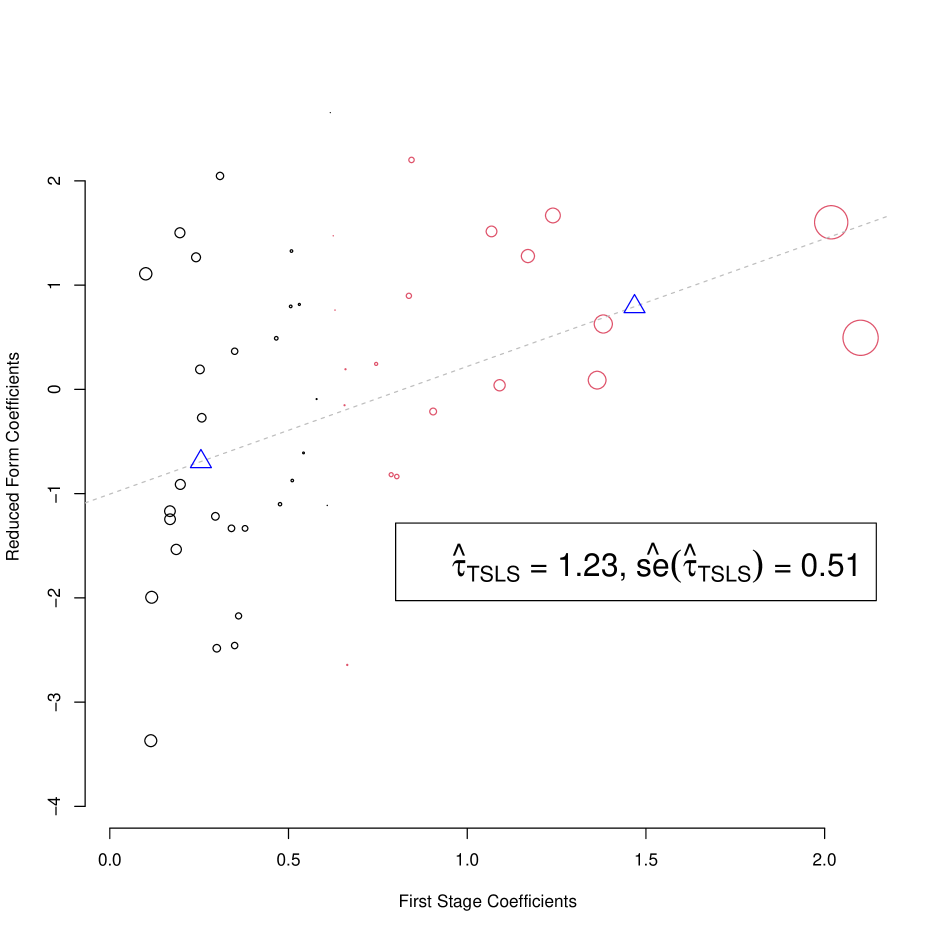
Panel A: Nakamura and Steinsson weights

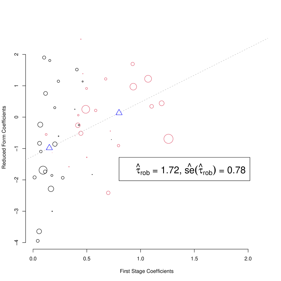
Panel B: Robust weights

Notes: This figure shows the state-level reduced-form and first-stage coefficients for Nakamura and Steinsson (2014) data. Circle sizes reflect the absolute value of weights; negative weights are printed in black, and positive – in red. Blue triangles are centers of mass for negative and positive weights. Panel A presents the results using the whole period of 1968 to 2006 for $n=48$ states. Panel B shows the results from our estimation algorithm. Under our data splitting procedure, Panel B reports the results for 1978-2006, as we use the first $1/3$ of the data for weight estimation.

Figure 2: Aggregate time-series data for Nakamura and Steinsson (2014) data

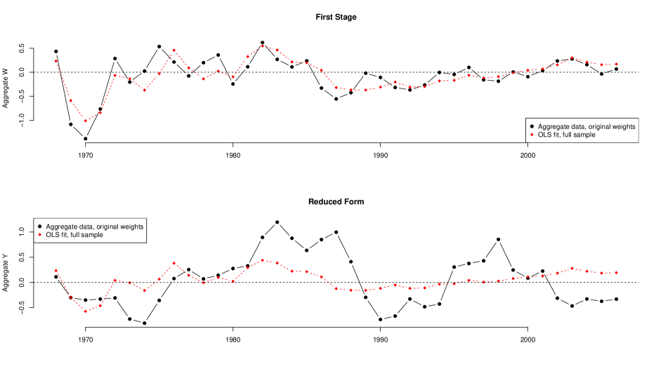
Panel A: Aggregation over $n=48$ states with original weights

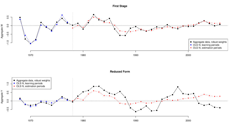
Panel B: Aggregation over $n=48$ states with robust weights

Notes: Solid lines represent aggregate data for different weights; dashed lines represent OLS predictions of the aggregate data with the instrument. The mean absolute value of weights is scaled to $1$.

2.2 New Estimator

Representation (2.3) shows that $\hat{\tau}_{TSLS}$ is a weighted combination of the unit-level coefficients $\{(\hat{\pi}_{i}^{OLS},\hat{\delta}_{i}^{OLS})\}_{i\leq n}$ with weights proportional to $D_{i}-\frac{1}{n}\sum_{j\leq n}D_{j}$. These weights sum up to zero, meaning that the TSLS estimator subtracts the weighted average of the units with relatively large exposures from those with relatively small ones. This is reflected in Panel A of Figure 1, where we use different colors for states with positive and negative weights.

This particular aggregation scheme is a consequence of the two-way model:

$$Y_{it}=\alpha_{i}^{(y)}+\mu_{t}^{(y)}+\tau W_{it}+\epsilon_{it}.$$ (2.6)

By averaging over the cross-sectional dimension with the weights that sum up to zero, we eliminate the time fixed effects. In applications, these effects capture unobserved aggregate shocks potentially correlated with $Z_{t}$. For example, in Nakamura and Steinsson (2014) time fixed effects are meant to capture other policy variables that are likely correlated with national procurement.

This strategy is appropriate only if potential unobserved shocks affect all cross-sectional units in the same way (or, at least, in a way that is unrelated to $D_{i}$). Thus the main threat to the validity of the TSLS estimator is the presence of aggregate confounders $H_{t}$ with heterogeneous coefficients:

$$Y_{it}=\alpha_{i}^{(y)}+\mu_{t}^{(y)}+\tau W_{it}+\theta_{i}H_{t}+\epsilon_{it}.$$ (2.7)

As long as $\theta_{i}$ is correlated with $D_{i}$ and $H_{t}$ is correlated with $Z_{t}$ the TSLS estimator suffers from the omitted variable bias (OVB) and is invalid. Applied researchers recognize this threat (e.g., see discussions in Guren et al., 2020; Chodorow-Reich et al., 2021) and address it by including additional aggregate and unit-specific control variables. Of course, in practice, we cannot guarantee that these controls are sufficient to account for all confounders.

Our estimator complements this strategy by using a more flexible weighting scheme. To understand why weighting can help with unobserved confounders, suppose $D_{i}$ is binary and split all units into two groups accordingly. If the average value of $\theta_{i}$ varies between these groups, then the TSLS strategy is invalid. If, however, there is an overlap in distributions of $\theta_{i}$ in the two groups, then we can correct these differences by reweighting. We cannot follow this strategy directly because $\theta_{i}$ is unknown. We can, however, use the observed data to implement it indirectly by searching for weights with certain balancing properties. This is the main idea behind the algorithm we present next.

First, we compute the state-level coefficients using data from the second part of the sample. Formally, for each unit $i$, we estimate equations

$$Y_{it}=\alpha_{i}^{(y)}+\delta_{i}Z_{t}+u_{it}^{(y)},$$ (2.8)

$$W_{it}=\alpha_{i}^{(w)}+\pi_{i}Z_{t}+u_{it}^{(w)},$$

by OLS using data for periods $t=T_{0}+1,\dots,T$. We use $\left\{\left(\hat{\pi}_{i}^{OLS,(T_{0}:T]},\hat{\delta}_{i}^{OLS,(T_{0}:T]}\right)\right\}_{i\leq n}$ to denote the corresponding OLS estimates. $T_{0}$ is a user-specified parameter, with a default value $T_{0}=\frac{T}{3}$.

To estimate the effect, we aggregate the coefficients using weights $\omega^{rob}_{i}$,

$$\hat{\tau}_{rob}=\frac{\sum_{i\leq n}\hat{\delta}_{i}^{OLS,(T_{0}:T]}\omega^{rob}_{i}}{\sum_{i\leq n}\hat{\pi}_{i}^{OLS,(T_{0}:T]}\omega^{rob}_{i}},$$ (2.9)

which we define below. Similarly to $\hat{\tau}_{TSLS}$, this estimator is numerically equal to the time-series IV estimator for the equation

$$Y_{t}^{rob}=\alpha+\tau W_{t}^{rob}+\epsilon_{t},$$ (2.10)

where $Y_{t}^{rob}:=\frac{1}{n}\sum_{i\leq n}Y_{it}\omega^{rob}_{i}$ and $W_{t}^{rob}:=\frac{1}{n}\sum_{i\leq n}Y_{it}\omega^{rob}_{i}$, we use $Z_{t}$ as an instrument, and estimate (2.10) using data for $t=T_{0}+1,\dots,T$. Using weights $\omega^{rob}_{i}$ as opposed to $D_{i}-\frac{1}{n}\sum_{j\leq n}D_{j}$ is the main conceptual difference between our estimator and the TSLS. Analogously to $\hat{\tau}_{TSLS}$, one can compute $\hat{\tau}_{rob}$ by estimating the equation

$$Y_{it}=\alpha_{i}+\mu_{t}+\tau W_{it}+\epsilon_{it}$$ (2.11)

by the TSLS for periods $t=T_{0}+1,\dots,T$, using $\omega^{rob}_{i}Z_{t}$ as an instrument.

We construct the weights $\omega^{rob}_{i}$ using the first $T_{0}$ periods. As discussed before, we want to make units with high values of $D_{i}$ look similar on average to those with low values of $D_{i}$. To this end, we residualize the data for each unit with respect to $Z_{t}$ and look for such a combination. We achieve this goal by solving a quadratic optimization problem:

$$(\omega^{rob},\hat{\eta}_{0}^{(w)},\hat{\eta}_{z}^{(w)},\hat{\eta}_{0}^{(y)},\hat{\eta}_{z}^{(y)})=\operatorname*{arg\,min}_{\{w,\eta_{0}^{(w)},\eta_{z}^{(w)},\eta_{0}^{(y)},\eta_{z}^{(y)}\}}\Bigg{\{}\frac{\zeta^{2}\|w\|_{2}^{2}}{nT_{0}}+$$ (2.12)

$$\frac{\frac{1}{T_{0}}\sum_{t\leq T_{0}}\left(\frac{1}{n}\sum_{i\leq n}w_{i}Y_{it}-\eta_{0}^{(y)}-\eta_{z}^{(y)}Z_{t}\right)^{2}}{\hat{\sigma}^{2}_{y,T_{0}}}+\frac{\frac{1}{T_{0}}\sum_{t\leq T_{0}}\left(\frac{1}{n}\sum_{i\leq n}w_{i}W_{it}-\eta_{0}^{(w)}-\eta_{z}^{(w)}Z_{t}\right)^{2}}{\hat{\sigma}^{2}_{w,T_{0}}}\Bigg{\}}$$

$$\text{subject to: }\frac{1}{n}\sum_{i\leq n}w_{i}D_{i}=1,\quad\frac{1}{n}\sum_{i\leq n}w_{i}=0,$$

where $\zeta^{2}$ is a user-specified regularization parameter, and

$$\hat{\sigma}^{2}_{y,T_{0}}:=\min_{\{\alpha_{i},\gamma_{i},\mu_{t}\}_{i,t}}\left\{\frac{\sum_{i\leq n,t\leq T_{0}}(Y_{it}-\alpha_{i}-\mu_{t}-\gamma_{i}Z_{t})^{2}}{nT_{0}}\right\},$$ (2.13)

$$\hat{\sigma}^{2}_{w,T_{0}}:=\min_{\{\alpha_{i},\gamma_{i},\mu_{t}\}_{i,t}}\left\{\frac{\sum_{i\leq n,t\leq T_{0}}(W_{it}-\alpha_{i}-\mu_{t}-\gamma_{i}Z_{t})^{2}}{nT_{0}}\right\}.$$

As a default value, we use

$$\zeta=\frac{\log(T_{0})\max\{\|\hat{\epsilon}^{(y)}\|_{op},\|\hat{\epsilon}^{(w)}\|_{op}\}}{\sqrt{nT_{0}}},$$ (2.14)

where $\hat{\epsilon}^{(y)}$ and $\hat{\epsilon}^{(w)}$ are $n\times T_{0}$ matrices of residuals from regressions in (2.13). The estimation procedure is summarized in Algorithm 1.

To gain intuition behind the optimization problem (2.12) it is useful to consider several edge cases. First, if $\zeta$ is equal to infinity, then $\omega^{rob}_{i}\propto(D_{i}-\frac{1}{n}\sum_{j\leq n}D_{j})$, i.e., we get the same aggregate variables as before. The resulting estimator is similar but not numerically equal to $\hat{\tau}_{TSLS}$ because we only use periods $t>T_{0}$ to estimate the coefficients.

To understand what happens when $\zeta\neq\infty$ suppose $D_{i}$ is binary, $D_{i}\in\{0,1\}$. As discussed before, the original aggregation scheme constructs a difference between average exposed ($D_{i}=1$) and not exposed ($D_{i}=0$) units. Aggregation with weights $\omega^{rob}_{i}$ has a similar flavor but corresponds to taking a weighted average in both groups. This follows from examining the constraint in (2.12). Among all possible weighted averages, we select the one that makes aggregate variables $Y_{t}^{rob}$ and $W_{t}^{rob}$ as predictable as possible. Motivation for this is evident from looking at the first-stage and the reduced-form equations that correspond to (2.7):

$$Y_{it}=\alpha_{i}^{(y)}+\mu_{t}^{(y)}+\delta D_{i}Z_{t}+\theta_{i}^{(y)}H_{t}+u_{it}^{(y)},$$

$$W_{it}=\alpha_{i}^{(w)}+\mu_{t}^{(w)}+\pi D_{i}Z_{t}+\theta_{i}^{(w)}H_{t}+u_{it}^{(w)}.$$

Unobserved confounders make the prediction of $Y_{it}$ and $W_{it}$ by $Z_{t}$ harder, so the weights that eliminate such factors should also make the prediction easier. Terms $u_{it}^{(y)}$ and $u_{it}^{(w)}$ create a statistical challenge – it is possible that instead of eliminating the confounder, the weights produce a combination of errors that compensates $H_{t}$. To prevent such overfitting, we include the regularization term in (2.12), which forces the weights to be as uniform as possible. Using this we can show that $\omega^{rob}$ are close to determinstic weights $\omega^{\star}$ which minimize

$$\sum_{t\leq T_{0}}\mathbb{E}\left(\frac{1}{n}\sum_{i\leq n}w_{i}Y_{it}-\eta_{0}^{(y)}-\eta_{z}^{(y)}Z_{t}\right)^{2}+\sum_{t\leq T_{0}}\mathbb{E}\left(\frac{1}{n}\sum_{i\leq n}w_{i}W_{it}-\eta_{0}^{(w)}-\eta_{z}^{(w)}Z_{t}\right)^{2},$$ (2.15)

subject to the same constraints. As long as $\frac{1}{n}\sum_{i\leq n}\omega^{\star}_{i}\theta_{i}^{(w)}$ and $\frac{1}{n}\sum_{i\leq n}\omega^{\star}_{i}\theta_{i}^{(y)}$ are small, we can expect $\frac{1}{n}\sum_{i\leq n}\omega^{rob}_{i}\theta_{i}^{(w)}$, and $\frac{1}{n}\sum_{i\leq n}\omega^{rob}_{i}\theta_{i}^{(y)}$ to be neglible as well. In Section 3 we present a large class of statistical models where this is indeed the case.

Data: $\{Y_{it},W_{it}\}_{it},\{D_{i}\}_{i\leq n},\{Z_{t}\}_{t\leq T},T_{0},\zeta$

Result: Estimates $(\hat{\pi}_{rob},\hat{\delta}_{rob},\hat{\tau}_{rob})$

1 Construct the unit weights $\{\omega^{rob}_{i}\}_{i\leq n}$ by solving optimization problem (2.12);

2 for $t\leftarrow T_{0}+1$ to $T$ do

3       Construct $Y_{t}^{rob}=\frac{1}{n}\sum_{i\leq n}Y_{it}\omega^{rob}_{i}$, and $W_{t}^{rob}=\frac{1}{n}\sum_{i\leq n}W_{it}\omega^{rob}_{i}$.

4      

5 end for

6Using the data for $t>T_{0}$, estimate two regressions by OLS:

$$Y_{t}^{rob}=\eta^{(y)}_{0}+\delta Z_{t}+\varepsilon_{t}^{(y)},\quad W_{t}^{rob}=\eta^{(w)}_{0}+\pi Z_{t}+\varepsilon_{t}^{(w)},$$

and report $\hat{\delta}_{rob}$, $\hat{\pi}_{rob}$, $\hat{\tau}_{rob}:=\frac{\hat{\delta}_{rob}}{\hat{\pi}_{rob}}$;

Algorithm 1 Estimation algorithm

2.3 Applying Robust Estimator

To implement our estimator for Nakamura and Steinsson (2014), we use the original exposures $D_{i}$, set $T_{0}=10$ (which corresponds to years 1968-1977), and use the default value for $\zeta$. We then construct $\omega^{rob}_{i}$ and estimate $\hat{\tau}_{rob}$ using Algorithm 1.

Panel B of Figure 1 plots the cross-sectional representation of our estimator. As before, the points represent the state-level first-stage and reduced-form coefficients but are now estimated using data from 1978 to 2006. The circle size reflects the absolute value of $\omega^{rob}_{i}$, and the colors reflect the sign. Our estimator $\hat{\tau}_{rob}=1.72$ equals the slope of the line connecting two centers of mass (blue triangles) for negative and positive weights. Compared to coefficients from Panel A of Figure 1, the first-stage coefficients computed for 1981-2006 exhibit less variability. By construction, in Panel A, the states with extreme first-stage coefficients have the largest weights (in absolute value), which is no longer the case in Panel B. Aggregating these state-level coefficients, we get a larger multiplier than before, though still within the range Nakamura and Steinsson (2014) report for alternative specifications.

There are two differences between Panel A and B of Figure 1. The first is the period we use to construct the state-level coefficients; the second is the weighting scheme. If we only change the period but apply the same weights as before, then we get a multiplier of $1.71$, with a standard error of $1.20$. The similarity between point estimates is not surprising, given visually minor differences between the weights, which we plot in Figure 3. The differences are mostly in the tails, with the original weights being extreme for several states. As a result, the standard error of the alternative estimator is $54\%$ higher.

We can see this in Panel B of Figure 2, which demonstrates the time-series representation of our estimator. We plot the aggregate data $Y_{t}^{rob}$ and $W_{t}^{rob}$ vis-a-vis two separate OLS predictions for years $1968-1977$ (in blue), and $1978-2006$ (in red). By changing the aggregation scheme, we reduce the variability: there is an $11\%$ reduction in the standard deviation for $W_{t}$, and $24\%$ – for $Y_{t}$. Despite this decrease in variability, aggregate instrument $Z_{t}$ remains relevant. Focusing only on periods $1979-2006$, the $R^{2}$ for $W_{t}$ increases from $54\%$ to $74\%$, and for $Y_{t}$ – from $11\%$ to $20\%$.

The higher, compared to the original estimate from Nakamura and Steinsson (2014), standard error of our estimator, $\hat{\text{s.e.}}(\hat{\tau}_{rob})=0.78$, is explained by a shorter time span, and relatively higher variability in $Z_{t}$ in the initial periods. We calculate this error by clustering at a yearly level in the TSLS regression

$$Y_{it}=\alpha_{i}+\mu_{t}+\tau W_{it}+\epsilon_{it},$$

where we use $\omega^{rob}_{i}Z_{t}$ as the instrument, and years $1978-2006$.

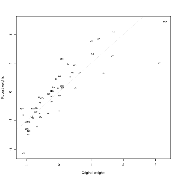
Figure 3: Scatterplot—Nakamura and Steinsson weights and robust weights

Notes: Scatter plot of original and robust weights for Nakamura and Steinsson (2014) data; $n=48$, state abbreviations are used as labels. The variance of weights is scaled to $1$.

2.4 Discussion

$\hat{\tau}_{TSLS}$ and $\hat{\tau}_{rob}$ rely on aggregation of the unit-level coefficients. We encourage users to produce analogs of Figure 1 to investigate the importance of alternative aggregation schemes. In applications where the unit-level coefficients exhibit strong association, the aggregation does not play a major role, resulting in similar estimates. If, however, there is significant variation, then the weighting scheme becomes important. In the rest of the paper, we demonstrate the advantages of our scheme with theory and simulations. At the same time, as with any method, our approach has its limitations and should be used carefully. Below we discuss the main ones, thus defining practical use cases for our estimator.

Our algorithm is data-intensive, particularly in the time dimension. Our formal results require the total number of periods to be large and the number of units $n$ to be at least of a similar order. Both of these assumptions can be restrictive in practice: in applied macroeconomics, we might observe relatively long time series for only a few units (e.g., monthly data for the states); in applied microeconomics, the number of observed periods is sometimes relatively small.

The second limitation is the flip side of the first one: for our weights to improve over the TSLS ones, the environment should be sufficiently stable over time. To construct $\omega^{rob}$ we use the residuals after projecting out $Z_{t}$, which behave well when the effect of $Z_{t}$ does not change over time. We return to this point in Section 4.2, where we discuss heterogeneous effects in more detail. For our weights to be useful for the second part of the data, any potential confounder like $H_{t}$ in (2.7) should have a similar effect in both data parts. This assumption might be too strong in environments where structural shocks are likely. This limitation can potentially be relaxed by using the whole sample to construct the weights. However, our theoretical results, particularly inference, rely on sample splitting. We also believe that sample splitting is a good general practice that protects from potential abuse.

Finally, our method is designed for applications in which the TSLS regression (1.1) is a priori reasonable, but the users are worried about potential unobserved confounders. There are multiple reasons why (1.1) might fail, other than omitted variables. For example, the underlying model can be nonlinear or the dynamic effects of the past treatments can be sizable. In these cases, the TSLS regression, and by extension, our improvement upon it, might be the wrong tool, and researchers should use other methods. We discuss this issue in more detail in Section 3 when we introduce a formal model.

Given these limitations, we recommend that applied researchers use our technique in situations where the number of observed periods is relatively large, structural shocks are unlikely, and the main potential problem is the presence of unobserved aggregate confounders rather than nonlinearity or dynamics. As we show with our formal results and simulations, our method either dominates the TSLS or performs similarly under this set of assumptions.

3 Theoretical analysis

We formulate three theoretical results in this section. The first theorem shows that our estimator remains consistent when the TSLS fails. The second postulates that our estimator is asymptotically unbiased and normal under mild technical assumptions. The third theorem justifies conventional inference in situations with sufficient heterogeneity in the baseline outcomes.

3.1 Setup

We observe $n$ units ($i$ is a generic unit) over $T$ periods ($t$ is a generic period). For each unit, we observe an outcome variable $Y_{it}$, an endogenous policy variable (treatment) $W_{it}$, an aggregate shock $Z_{t}$, and a measure of exposure of unit $i$ to this shock $D_{i}$. We aim to estimate a causal relationship between $Y_{it}$ and $W_{it}$. To formalize causality, we start with a model of potential outcomes (Neyman, 1923; Rubin, 1977). In addition to $w_{t}$ (potential value of $W_{it}$) and $z_{t}$ (potential value of $Z_{t}$), we also introduce $h_{t}$ – an unobserved aggregate shock that causally affects both the outcome and the treatment variable. We define $w^{t}:=(\dots,w_{1},\dots,w_{t})$, $z^{t}:=(\dots,z_{1},\dots,z_{t})$, and $h^{t}:=(\dots,h_{1},\dots,h_{t})$, and make our first assumption.

Assumption 3.1.

(Potential outcomes)
Potential outcomes follow a static linear model:

$$Y_{it}(w^{t},h^{t})=\alpha^{(y)}_{it}+\tau w_{t}+\theta^{(y)}_{i}h_{t},$$ (3.1)

$$W_{it}(h^{t},z^{t})=\alpha_{it}^{(w)}+\pi_{i}z_{t}+\theta^{(w)}_{i}h_{t}.$$

As a result, the realized outcomes satisfy

$$Y_{it}=\alpha^{(y)}_{it}+\tau W_{it}+\theta^{(y)}_{i}H_{t},$$ (3.2)

$$W_{it}=\alpha_{it}^{(w)}+\pi_{i}Z_{t}+\theta^{(w)}_{i}H_{t}.$$

The critical part of this assumption and our setup overall is the unobserved aggregate variable $H_{t}$. The danger such unobservables present for identification is well-recognized in applied work (e.g., Chodorow-Reich et al., 2021). The typical restriction made in the literature is to assume that $\theta_{i}^{(w)},\theta_{i}^{(y)}$ do not vary over $i$ in a systematic way. We do not make this assumption and instead allow for such heterogeneity. Following most empirical applications, we focus on contemporaneous treatment effects and assume that only current quantities affect the outcomes. Finally, to simplify the exposition, we assume away heterogeneity in treatment effects. We relax this in Section 4 where we discuss when the output of our algorithm can be interpreted as a weighted average of individual treatment effects.

Our next assumption describes the relation between the aggregate variables and the potential outcomes.

Assumption 3.2.

(Exogeneity)
Aggregate shocks are independent of potential outcomes:

$$\{Z_{t},H_{t}\}_{t\leq T}\mathchoice{\mathrel{\hbox to0.0pt{$\displaystyle\perp$\hss}\mkern 2.0mu{\displaystyle\perp}}}{\mathrel{\hbox to0.0pt{$\textstyle\perp$\hss}\mkern 2.0mu{\textstyle\perp}}}{\mathrel{\hbox to0.0pt{$\scriptstyle\perp$\hss}\mkern 2.0mu{\scriptstyle\perp}}}{\mathrel{\hbox to0.0pt{$\scriptscriptstyle\perp$\hss}\mkern 2.0mu{\scriptscriptstyle\perp}}}\{\alpha^{(w)}_{it},\alpha^{(y)}_{it},\theta^{(y)}_{i},\theta^{(w)}_{i},\pi_{i}\}_{i\leq n,t\leq T}.$$ (3.3)

Assumption 3.2 is natural in applications where $Z_{t}$ and $H_{t}$ can be plausibly considered exogenous, i.e., determined outside the relevant model for the unit-level outcomes. For example, suppose $(Y_{it},W_{it})$ are determined jointly in the local equilibrium:

$$Y_{it}=\alpha_{it}^{(y)}+\tau W_{it}+\theta^{(y)}_{i}H_{t},$$ (3.4)

$$W_{it}=\alpha_{it}^{(w)}+\gamma Y_{it}+\pi_{i}Z_{t}.$$

This structure arises, for example, in Guren et al. (2020) where $Y_{it}$ is the retail employment in location $i$, period $t$, and $W_{it}$ is the house price. The aggregate variables correspond to exogenous demand and supply shifters. Substituting $Y_{it}$ in the expression for $W_{it}$ we get the model (3.1). This example demonstrates the difference between $Z_{t}$ and $H_{t}$. The former acts as a shifter for $W_{it}$ and is excluded from the structural equation for $Y_{it}$. Despite this exclusion restriction, $Z_{t}$ might be an invalid instrument due to its potential correlation with $H_{t}$.

The presence of the unobserved shock $H_{t}$ makes the causal model described by Assumption 3.1 and 3.2 somewhat nonstandard. To see this, define $Y_{it}(w):=Y_{it}(w,H_{t})$ and $W_{it}(z):=W_{it}(z,H_{t})$ – potential outcomes at realized values of $h_{t}$. For each $i$, $\{Y_{it}(w),W_{it}(z)\}_{t\leq T}$ is a version of the conventional IV model of Imbens and Angrist (1994). In particular, Assumption 3.1 guarantees that the instrument $Z_{t}$ satisfies the exclusion restriction for each unit. Assumption 3.2, however, does not guarantee that $Z_{t}$ is independent of $(Y_{it}(w),W_{it}(z))$. The two assumptions together quantify the extent of this dependence at the unit level:

$$\mathbb{E}\left[Y_{it}(w)(Z_{t}-\mathbb{E}[Z_{t}])|\alpha_{it}^{(w)},\alpha_{it}^{(y)},\pi_{i},\theta_{i}^{(w)},\theta_{i}^{(y)}\right]=\theta_{i}^{(y)}\mathbb{E}[H_{t}(Z_{t}-\mathbb{E}[Z_{t}])],$$ (3.5)

$$\mathbb{E}\left[W_{it}(z)(Z_{t}-\mathbb{E}[Z_{t}])|\alpha_{it}^{(w)},\alpha_{it}^{(y)},\pi_{i},\theta_{i}^{(w)},\theta_{i}^{(y)}\right]=\theta_{i}^{(w)}\mathbb{E}[H_{t}(Z_{t}-\mathbb{E}[Z_{t}])].$$

We thus relax the independence assumption of Imbens and Angrist (1994) (Condition 1, (i) in the paper) but impose a product structure on the correlation. This structure is motivated by applications where it is plausible to view $Z_{t}$ as exogenous (in the sense of Assumption 3.2), but other aggregate shocks might also affect the outcomes. In other words, the first stage and the reduced form can suffer from the omitted variable bias, where the confounder varies over time but not over units.

In practice, we cannot guarantee that $H_{t}$ is one-dimensional, and thus a model with multiple unobserved shocks might be more appropriate. Conceptually, this extension is straightforward since we can interpret $(\theta_{i}^{(y)},\theta_{i}^{(w)})$ and $H_{t}$ as $p$-dimensional vectors. For $p$ large enough the RHS of (3.5) can approximate arbitrary covariance between $Y_{it}(w),\,W_{it}(z)$ and $Z_{t}$. The dimension of $H_{t}$ does not directly enter Algorithm 1 but makes its analysis more involved. To simplify the exposition, we focus on the one-dimensional case, which transmits theoretical insights in the simplest form. In Appendix B.2, we establish our main bound assuming $H_{t}$ is a vector, and later specialize it to the scalar case.

Our next assumption restricts the joint distribution of aggregate variables $\{(Z_{t},H_{t})\}_{t\leq T}$. Since they serve as a source of quasi-experimental variation in our setup, we call it a design model.

Assumption 3.3.

(Design model)
The aggregate variables $(Z_{t},H_{t})$ follow a time-heterogeneous linear process. In particular, they satisfy

$$Z_{t}=\eta_{z}+\epsilon_{t}^{(z)},\quad H_{t}=\eta_{h}+\epsilon_{t}^{(h)}.$$ (3.6)

For $k\in\{z,h\}$ define $\epsilon^{(k)}:=(\epsilon^{(k)}_{T},\dots,\epsilon^{(k)}_{1})^{\top}$; there exist $T$-dimensional vectors $\nu^{(z)},\nu^{(h)}$, two upper-triangular matrices $\Lambda^{(z)},\Lambda^{(h)}$, and $\rho_{ag}\in(-1,1)$ such that

$$\epsilon^{(z)}=\Lambda^{(z)}\nu^{(z)},\quad \epsilon^{(h)}=\Lambda^{(h)}(\rho_{ag}\nu^{(z)}+\sqrt{(1-\rho_{ag}^{2})}\nu^{(h)}).$$ (3.7)

Vectors $\nu^{(z)},\nu^{(h)}$ are independent, have independent components with the uniformly bounded sub-gaussian norm, and $\mathbb{E}\left[(\nu_{t}^{(z)})^{2}\right]=\mathbb{E}\left[(\nu_{t}^{(h)})^{2}\right]=1$. For $k\in\{z,h\}$ and $j\leq T$ we have

$$0<\sigma_{\min}\leq(\Lambda^{(k)})_{jj}\leq\sigma_{\max}<\infty,\quad\left|(\Lambda^{(k)})_{jl}\right|\leq\frac{\rho_{\max}}{(l-j)^{2}},\text{ for $l>j$}.$$ (3.8)

The first part of this assumption restricts the means of $Z_{t}$ and $H_{t}$, which are assumed to be constant over time. This is without loss of generality for $H_{t}$, because its mean can be treated as a part of $\alpha_{it}^{(w)}$ and $\alpha_{it}^{(y)}$, but it is restrictive for $Z_{t}$. This assumption can be relaxed by considering a parametric model for the mean, e.g., allowing for seasonality or secular trends. Fundamentally, our approach relies on the fact that researchers know how to detrend $Z_{t}$ and exploit random fluctuations $\epsilon_{t}^{(z)}$, which is particularly easy if the mean is constant. This idea is closely connected to Borusyak and Hull (2020), where the authors show that such de-meaning is crucial for design-based methods.

The second part restricts the distribution of $\epsilon^{(z)}$ and $\epsilon^{(h)}$. These errors are generated by the underlying independent structural shocks $\nu^{(z)}$ and $\nu^{(h)}$. Since $\rho_{ag}$ is less than one, there is variation in $\epsilon^{(h)}_{t}$ that is not entirely explained by $\epsilon^{(z)}_{t}$ (and vice versa). Restrictions on the elements of matrices $\Lambda^{(z)},\Lambda^{(h)}$ exclude persistent cases (e.g., random walks) but allow for other forms of non-stationarity.

The next two assumptions restrict heterogeneity in potential outcomes. We start with exposures $\pi_{i}$, connecting them to observed $D_{i}$.

Assumption 3.4.

(Strong Instruments)
There exist numbers $(\eta_{0},\eta_{\pi})$ with $\eta_{\pi}\neq 0$, such that for every $i$ we have $\pi_{i}=\eta_{0}+\eta_{\pi}D_{i}$.

This assumption guarantees that $D_{i}Z_{t}$ is a relevant predictor for $W_{it}$, making it a “strong” instrument. The linearity is motivated by the empirical practice where researchers often assume that exposures $\pi_{i}$ are known up to linear transformation (e.g., Dube and Vargas, 2013; Nunn and Qian, 2014). Fundamentally, our theoretical results rely on $D_{i}$ being strongly correlated with $\pi_{i}$ after adjusting for other unit-specific coefficients. As a result, one can extend Assumption 3.4 by explicitly including $\theta_{i}^{(w)},\theta_{i}^{(y)}$ or functions of $\{\alpha_{it}^{(w)},\alpha_{it}^{(y)}\}_{t\leq T}$ in the expression for $\pi_{i}$.

To state our next assumption, we introduce additional notation. For any $T_{a}>1$ define population analogs of $\hat{\sigma}_{k,T_{0}}$ from (2.13):

$$\sigma^{2}_{y,T_{a}}:=\min_{\{\alpha_{i},\gamma_{i},\mu_{t}\}_{i,t}}\left\{\frac{\sum_{i\leq n,t\leq T_{a}}\mathbb{E}_{H,Z}[(Y_{it}-\alpha_{i}-\mu_{t}-\gamma_{i}Z_{t})^{2}]}{nT_{a}}\right\},$$ (3.9)

$$\sigma^{2}_{w,T_{a}}:=\min_{\{\alpha_{i},\gamma_{i},\mu_{t}\}_{i,t}}\left\{\frac{\sum_{i\leq n,t\leq T_{a}}\mathbb{E}_{H,Z}[(W_{it}-\alpha_{i}-\mu_{t}-\gamma_{i}Z_{t})^{2}]}{nT_{a}}\right\}.$$

For any $T_{b}>T_{a}\geq 1$, $t\in[T_{a},T_{b}]$, weights $\omega_{i}$ such that $\sum_{i\leq n}\omega_{i}=0$, and $k\in\{y,w\}$ define:

$$\alpha_{t,T_{a}|T_{b}}^{(k)}(\omega):=\frac{1}{n\sqrt{T_{b}-T_{a}+1}}\sum_{i\leq n}\omega_{i}\left(\alpha_{it}^{(k)}-\frac{1}{T_{b}-T_{a}+1}\sum_{T_{a}\leq l<T_{b}}\alpha_{il}^{(k)}\right).$$ (3.10)

As mentioned in Section 2, our results rely on the fact that the weights $\omega^{rob}$ are close to deteriminstic oracle weights $\omega^{\star}$ that optimize the expected version of (2.12):

$$\frac{1}{T_{0}\sigma^{2}_{y,T_{0}}}\sum_{t\leq T_{0}}\mathbb{E}\left(\frac{1}{n}\sum_{i\leq n}w_{i}Y_{it}-\eta_{0}^{(y)}-\eta_{z}^{(y)}Z_{t}\right)^{2}+\\ \frac{1}{T_{0}\sigma^{2}_{y,T_{0}}}\sum_{t\leq T_{0}}\mathbb{E}\left(\frac{1}{n}\sum_{i\leq n}w_{i}W_{it}-\eta_{0}^{(w)}-\eta_{z}^{(w)}Z_{t}\right)^{2},$$ (3.11)

subject to appropriate constraints. Using Assumptions 3.1-3.4 we can compute these expectations, and after concentrating $\left\{\eta_{0}^{(k)},\eta_{z}^{(k)}\right\}_{k\in\{y,w\}}$ we get

$$\frac{\sum_{t\leq T_{0}}\left(\alpha_{t,1|T_{0}}^{(w)}(\omega)\right)^{2}+\kappa^{2}(T_{0})\left(\frac{1}{n}\sum_{i\leq n}\omega_{i}\theta_{i}^{(w)}\right)^{2}}{\sigma^{2}_{w,T_{0}}}+\\ \frac{\sum_{t\leq T_{0}}\left(\alpha_{t,1|T_{0}}^{(y)}(\omega)+\tau\alpha_{t,1|T_{0}}^{(w)}(\omega)\right)^{2}+\kappa^{2}(T_{0})\left(\frac{1}{n}\sum_{i\leq n}\omega_{i}(\theta_{i}^{(y)}+\tau\theta_{i}^{(w)})\right)^{2}}{\sigma^{2}_{y,T_{0}}},$$ (3.12)

where $\kappa^{2}(T_{0})$ is strictly positive.

Our final assumption guarantees that the oracle problem (3.12) has a well-behaved solution and allows us to exploit the cross-sectional dimension of the problem to achieve identification.

Assumption 3.5.

(Overlap)
For any $T_{a}>1$ there exist $\{\omega^{\star}_{i,T_{a}}\}_{i\leq n}$ such that

$$\sum_{k\in\{y,w\}}\left[\frac{\sum_{t\leq T_{a}}\left(\alpha_{t,1|T_{a}}^{(k)}(\omega^{\star}_{T_{a}})\right)^{2}+\left(\frac{1}{n}\sum_{i\leq n}\omega^{\star}_{T_{a}}\theta_{i}^{(k)}\right)^{2}}{\sigma^{2}_{k,T_{a}}}\right]\lesssim\frac{\log(n)}{n},$$ (3.13)

$$\frac{1}{n}\sum_{i\leq n}\omega^{\star}_{i,T_{a}}D_{i}=1,\quad\frac{1}{n}\sum_{i\leq n}\omega^{\star}_{i,T_{a}}=0,\quad\frac{1}{n}\sum_{i\leq n}\left(\omega^{\star}_{i,T_{a}}\right)^{2}\lesssim 1.$$

Assumption 3.5 guarantees the presence of variation in $D_{i}$ that is not captured by other unit-specific coefficients. It is similar to overlap assumptions commonly imposed in settings with unconfoundedness (e.g., Imbens and Rubin, 2015). Under Assumption 3.5, the more units we observe, the better we can “balance out” unobserved confounders using weights $\omega^{\star}_{T_{a}}$. We can eliminate them in the limit where $n$ converges to infinity. As a result, Assumption 3.5 guarantees that $\tau$ can be identified within the class of estimators we consider.

To justify Assumption 3.5 we now consider an example that encompasses many models used in current empirical practice.

Proposition 1.

Suppose that for $k\in\{y,w\}$

$$\alpha_{it}^{(k)}=\alpha_{i}^{(k)}+\mu_{t}^{(k)}+L_{it}^{(k)}+\epsilon_{it}^{(k)},$$ (3.14)

$$(\epsilon_{iT}^{(k)},\dots\epsilon_{i1}^{(k)})^{\top}=\left(\Sigma^{(k)}\right)^{\frac{1}{2}}\tilde{\epsilon}_{i}^{(k)},$$

$$\mathbb{E}[\epsilon_{i}^{(k)}]=\mathbf{0}_{T\times 1},\quad\mathbb{V}[\epsilon_{i}^{(k)}]=\mathcal{I}_{T},$$

where $\|\Sigma^{(k)}\|_{op}\lesssim 1$, $T$-dimensional vectors $\epsilon_{i}^{(k)}$ are independent over $i$, with independent uniformly bounded sub-gaussian components, and for any $t\in\{1,\dots,T\}$ $\frac{\sum_{i\leq n}\left(L_{it}^{(k)}\right)^{2}}{n}\lesssim 1$. In addition, suppose

$$D_{i}=\alpha_{i}^{(d)}+\epsilon_{i}^{(d)},\quad\mathbb{E}[\epsilon_{i}^{(d)}]=0,\quad\mathbb{V}[\epsilon_{i}^{(d)}]=\sigma^{2}_{d},$$ (3.15)

where $\frac{\sum_{i\leq n}(\alpha_{i}^{(d)})^{2}}{n}\lesssim 1$ and $\epsilon^{(d)}_{i}$ are independent over $i$, independent of $\epsilon_{i}^{(w)},\epsilon_{i}^{(y)}$, and have uniformly bounded sub-gaussian norm. Finally, suppose for $k\in\{y,w\}$ $\frac{\sum_{i\leq n}(\theta_{i}^{(k)})^{2}}{n}\lesssim 1$ and Assumption 3.3 holds. Then Assumption 3.5 holds for $\omega^{\star}_{i,T_{0}}\propto(\epsilon_{i}^{(d)}-\frac{1}{n}\sum_{j\leq n}\epsilon_{j}^{(d)})$ with probability approaching one as $n$ approaches infinity.

This example covers many familiar cases. First, if $\alpha_{i}^{(d)}=\alpha^{(d)}$, then $D_{i}$ is as good as randomly assigned – situation that rarely holds in applications, but serves as a natural benchmark. If $L_{it}^{(k)}\equiv 0$, then we recover a conventional two-way model that is commonly used in applications. In practice, we rarely expect the two-way model to hold exactly, and $L_{it}^{(k)}$ can be viewed as an approximation error. If $L_{it}^{(k)}$ has product structure, then we recover the interactive fixed effects model (e.g., Bai, 2009). However, this structure is not necessary, and $L_{it}^{(k)}$ can vary in an arbitrary way, as long as it remains appropriately bounded. The key part of the setup that allows us to construct $\omega^{\star}_{i,T_{0}}$ is the presence of $\epsilon_{i}^{(d)}$ – exogenous variation in $D_{i}$ that is unrelated to any other local-level parameters. Informally, to justify Assumption 3.5 in applications, researchers need to argue that there is some underlying randomness in $D_{i}$. We view this as a natural identification requirement.

3.2 Statistical Properties

We now turn to the statistical properties of our estimator. We use a design-based framework and all probability statements in the section except those in Proposition 2 refer to the joint distribution of $\{(Z_{t},H_{t})\}_{t\leq T}$. We focus on a particular asymptotic regime characterized by the next assumption.

Assumption 3.6.

(Asymptotic regime)
Both $n$ and $T$ increase to infinity and $\frac{T}{n}\rightarrow\gamma_{rat}<\infty$, for $k\in\{y,w\}$ we have

$$\frac{1}{n}\sum_{i\leq n}\left(\theta_{i}^{(k)}-\frac{1}{n}\sum_{j\leq n}\theta_{j}^{(k)}\right)^{2}\rightarrow\sigma^{2}_{\theta^{(k)}}>0,\quad\frac{1}{n}\sum_{i\leq n}\left(D_{i}-\frac{1}{n}\sum_{j\leq n}D_{j}\right)^{2}\rightarrow\sigma^{2}_{D}>0,$$ (3.16)

$$\frac{\frac{1}{n}\sum_{i\leq n}\left(D_{i}-\frac{1}{n}\sum_{j\leq n}D_{j}\right)\theta_{i}^{(k)}}{\sigma_{D}\sigma_{\theta^{(k)}}}\rightarrow\rho_{cs}^{(k)},\quad\frac{1}{n}\sum_{i\leq n}\left(\alpha_{it}^{(k)}\right)^{2}\rightarrow\left(\alpha_{t}^{(k)}\right)^{2},$$

$$0<\alpha_{\min}^{2}\leq\left(\alpha_{t}^{(k)}\right)^{2}\leq\alpha_{\max}^{2}<\infty.$$

With the first part of this assumption, we restrict the analysis to environments where $n$ is comparable to or larger than $T$, which we expect to hold in many applications. The second part implies that the variability in $D_{i}$ and $\theta_{i}^{(k)}$ is present in the limit. For binary $D_{i}$, this assumption is reasonable if the size of the treated or control group is not too small. The variability in $\theta_{i}^{(k)}$ implies that $H_{t}$ is a “strong” factor. While common in theoretical literature on interactive fixed effects (e.g., Bai, 2009; Moon and Weidner, 2015), this assumption can be restrictive in some applications, where researchers expect little variability in $\theta_{i}^{(k)}$. A version of our results holds in environments where $\sigma^{2}_{\theta^{(k)}}=0$ (see the discussion in Appendix B.3). The restriction on the correlation is innocuous, as it always holds along a subsequence, and we make it to simplify the exposition. Finally, the restriction on $\alpha^{(k)}_{it}$ guarantees that $Y_{it}$ and $W_{it}$ have finite variances.

Assumption 3.6 describes the limit behavior of unit-specific quantities. For the aggregate variables we define similar objects for fixed $T_{b}>T_{a}\geq 1$ and $k\in\{z,h\}$:

$$\sigma_{k,T_{a}|T_{b}}:=\sqrt{\frac{1}{T_{b}-T_{a}+1}\sum_{T_{a}\leq t<T_{b}}\mathbb{E}\left[\left(\epsilon_{t}^{(k)}-\frac{\sum_{T_{a}\leq l<T_{b}}\epsilon_{l}^{(k)}}{T_{b}-T_{a}+1}\right)^{2}\right]},$$ (3.17)

$$\rho_{T_{a}|T_{b}}:=\frac{\frac{1}{T_{b}-T_{a}+1}\sum_{T_{a}\leq t<T_{b}}\mathbb{E}\left[\left(\epsilon_{t}^{(z)}-\frac{\sum_{T_{a}\leq l<T_{b}}\epsilon_{l}^{(z)}}{T_{b}-T_{a}+1}\right)\epsilon_{t}^{(h)}\right]}{\sigma_{h,T_{a}|T_{b}}\sigma_{z,T_{a}|T_{b}}}.$$

As indicated by the indices, these quantities depend on $T_{a},T_{b}$. Assumption 3.3 guarantees that $|\rho_{T_{a}|T_{b}}|\leq 1$, and $\sigma_{k,T_{a}|T_{b}}$ are uniformly bounded from above and below.

Our first result compares probability limits of $\hat{\tau}_{TSLSL}$ and $\hat{\tau}_{rob}$.

Theorem 3.1.

(Consistency)
Suppose Assumption 3.1-3.6 hold, $\zeta^{2}=\log(T_{0})$, and $\frac{T_{0}}{T}\rightarrow\gamma_{T}\in(0,1)$, then

$$\hat{\tau}_{rob}=\tau+o_{p}(1).$$

If, in addition, $\left|\rho_{cs}^{(w)}\sigma_{\theta^{(w)}}\rho_{1|T}\sigma_{h,1|T}+\eta_{\pi}\sigma_{D}\sigma_{z,1|T}\right|>c_{\min}>0$, then

$$\hat{\tau}_{TSLS}=\tau+\frac{\rho_{cs}^{(y)}\sigma_{\theta^{(y)}}\rho_{1|T}\sigma_{h,1|T}}{\rho_{cs}^{(w)}\sigma_{\theta^{(w)}}\rho_{1|T}\sigma_{h,1|T}+\eta_{\pi}\sigma_{D}\sigma_{z,1|T}}+o_{p}(1).$$

This result demonstrates that $\hat{\tau}_{rob}$ remains consistent in the regime where $\hat{\tau}_{TSLS}$ generally fails. It also formalizes a part of the discussion in Section 2.4. In our model, the only threat to the validity of the TSLS is the presence of omitted variables. As long as either $\rho_{cs}^{(y)}$ or $\rho_{1|T}$ is equal to zero the TSLS estimator is consistent.

Theorem 3.1 provides a first justification for using our estimator, but it does not describe its distributional properties in large samples. Under current assumptions, we can only provide relatively weak guarantees on the asymptotic behavior of $\hat{\tau}_{rob}$. In particular, Assumptions 3.5, 3.6 imply that there exist weights such that

$$\left|\frac{1}{n}\sum_{i\leq n}\omega^{\star}_{i,T_{0}}\theta_{i}^{(k)}\right|\lesssim\sqrt{\frac{\log(T_{0})}{T_{0}}},$$

however, this property is too weak to achieve asymptotic unbiasedness. To make progress, we impose additional assumptions on $\theta_{i}^{(y)},\theta_{i}^{(w)}$.

Assumption 3.7.

(Sufficient heterogeneity)
For any $T_{a}>1$ and $k\in\{y,w\}$ there exists $\{\omega^{\star}_{k,i,T_{a}}\}_{i\leq n}$ such that

$$\sum_{l\in\{y,w\}}\left[\frac{\frac{1}{T_{a}}\sum_{t\leq T_{a}}\left(\alpha_{t,1|T_{0}}^{(k)}(\check{\omega}_{T_{a}}^{(k)})\right)^{2}}{\sigma^{2}_{l,T_{a}}}\right]+\frac{\left(\frac{1}{n}\sum_{i\leq n}\omega^{\star}_{k,i,T_{a}}\theta_{i}^{(-k)}\right)^{2}}{\sigma^{2}_{-k,T_{a}}}\lesssim\frac{\log(n)}{n},$$ (3.18)

$$\frac{1}{n}\sum_{i\leq n}\omega^{\star}_{k,i,T_{a}}\theta_{i}^{(k)}=\sqrt{\frac{1}{n}\sum_{i\leq n}\left(\theta_{i}^{(k)}-\frac{1}{n}\sum_{j\leq n}\theta_{j}^{(k)}\right)^{2}},\quad\frac{1}{n}\sum_{i\leq n}\omega^{\star}_{k,i,T_{a}}=0,\quad\frac{1}{n}\sum_{i\leq n}\left(\omega^{\star}_{k,i,T_{a}}\right)^{2}\lesssim 1.$$

This Assumption is formally similar to Assumption 3.5 and requires existence of variation in $\theta_{i}^{(k)}$ that is not captured by $\alpha_{it}^{(w)},\alpha_{it}^{(y)}$ and $\theta_{i}^{-(k)}$. To justify it, we return to the example from Proposition 1.

Proposition 2.

Suppose conditions of Proposition 1 hold. In addition, suppose for $k\in\{y,w\}$ we have

$$\theta_{i}^{(k)}=\alpha_{i}^{(k)}+\epsilon_{i}^{(k)},\quad\mathbb{E}[\epsilon_{i}^{(k)}]=0,\quad\mathbb{V}[\epsilon_{i}^{(k)}]=\sigma^{2}_{\theta^{(k)}},$$ (3.19)

where $\epsilon_{i}^{(k)}$ are independent over $i$, and $k$, and have uniformly bounded sub-gaussian norm. Then Assumption 3.7 holds with probability one as $n$ approaches infinity.

To understand why Assumption 3.7 can improve the performance of $\hat{\tau}_{rob}$ it is useful to consider environments where it fails. In particular, if $\theta_{i}^{(k)}$ is nearly spanned by $\{\alpha_{it}^{(y)},\alpha_{it}^{(w)}\}_{t\leq T_{0}}$ and $\theta_{i}^{(-k)}$, but the remaining variation is strongly associated with $\pi_{i}$, then it is very hard to eliminate it by aggregation which results in a slow rate of convergence. This problem is mitigated when there is enough variability in $\theta_{i}^{(k)}$, which is not explained by other variables. Our next result demonstrates these gains by characterizing the asymptotic behavior of $\hat{\tau}_{rob}$. To state it we define for arbitrary periods $T_{b}>T_{a}>0$ a matrix $\Lambda^{(z)}_{T_{a}|T_{b}}$ such that

$$(\epsilon^{(z)}_{T_{b}},\dots,\epsilon^{(z)}_{T_{a}})^{\top}=\Lambda^{(z)}_{T_{a}|T_{b}}\nu^{(z)}.$$ (3.20)

Theorem 3.2.

(Asymptotic behavior)
Suppose Assumption 3.1-3.7 hold, $\zeta^{2}=\log(T_{0})$, and $\frac{T_{0}}{T}\rightarrow\gamma_{T}\in(0,1)$. Then there exists deterministic weights $\{\omega^{det}_{i,T_{0}}\}_{i\leq n}$ such that $\frac{1}{\sqrt{n}}\|\omega^{rob}_{i}-\omega^{det}_{i,T_{0}}\|_{2}=o_{p}(1)$, and

$$\sqrt{T_{1}}\left(\hat{\tau}_{rob}-\tau\right)=\frac{\sigma_{n,T}}{\eta_{\pi}\sigma^{2}_{z,T_{0}+1|T}}\xi_{n}+o_{p}(1),\quad\mathbb{E}[\xi_{n}]=0,\quad\mathbb{V}[\xi_{n}]=1,$$ (3.21)

where $\sigma_{n,T}:=\left\|\alpha_{T_{0}+1|T}^{(y)}(\omega^{det}_{T_{0}})\Lambda^{(z)}_{T_{0}+1|T}\right\|_{2}$. If, in addition, $\frac{\|\alpha_{T_{0}+1|T}^{(y)}(\omega^{det}_{T_{0}})\|_{\infty}}{\|\alpha_{T_{0}+1|T}^{(y)}(\omega^{det}_{T_{0}})\|_{2}}=o(1)$, then $\xi_{n}$ converges in distribution to $\mathcal{N}(0,1)$.

This result implies that our estimator is asymptotically unbiased and normal as long as $\sigma_{n,T}$ remains bounded. This condition can be restrictive, e.g., if $\alpha_{it}^{(y)}\sim\mathcal{N}\left(\alpha^{(y)}_{i}+\lambda_{t}^{(y)},\sigma^{2}_{\alpha^{(y)}}\right)$, then $\sigma_{n,T}=O_{p}\left(\frac{1}{\sqrt{n}}\right)$ and higher order terms in (3.21) become important. This lack of uniformity is similar to one considered in Menzel (2021). In practice, we do not expect the two-way model to hold exactly and rather view it as an approximation. In this situation, the first term in (3.21) becomes dominant, and we can use Theorem 3.2 for inference.

Theorem 3.2 describes the asymptotic behavior of our estimator in the presence of unobserved shocks. If there are no such confounders in the structural equation, i.e., $\theta_{i}^{(y)}\equiv 0$, then our estimator and the standard TSLS estimator are asymptotically normal under mild technical conditions. In this regime, $\sigma_{n,T}$ can be smaller or larger than its TSLS counterpart $\left\|\alpha_{1|T}^{(y)}(\omega^{TSLS})\Lambda^{(z)}_{1|T}\right\|_{2}$ depending on the underlying complexity of the potential outcomes and differences in the sample sizes.

We conduct inference in several steps summarized in Algorithm 2. First, we estimate the variance. We assume that a researcher has access to a consistent estimator for $\Lambda^{(z)}_{T_{0}+1|T}$ which we denote $\hat{\Lambda}^{(z)}_{T_{0}+1|T}$. For $t>T_{0}$ we construct scaled residuals from the aggregate regression

$$\hat{\alpha}_{t,T_{0}|T}^{(y)}(\omega^{rob}):=\frac{Y_{t}^{rob}-\hat{\tau}_{rob}W_{t}^{rob}}{\sqrt{T_{1}}},$$ (3.22)

and estimate the asymptotic standard error of $\hat{\tau}_{rob}$:

$$\hat{\sigma}_{rob}:=\frac{\|\hat{\alpha}_{T_{0}+1|T}^{(y)}(\omega^{rob})\hat{\Lambda}^{(z)}_{T_{0}+1|T}\|_{2}}{|\hat{\pi}_{rob}|\frac{1}{T_{1}}\sum_{T_{0}<t<T}\left(Z_{t}-\frac{\sum_{T_{0}<l\leq T}Z_{l}}{T_{1}}\right)^{2}}.$$ (3.23)

With this quantity, we construct a standard asymptotic confidence interval of level $1-\alpha$:

$$\tau\in\hat{\tau}_{rob}\pm\frac{\hat{\sigma}_{rob}}{\sqrt{T_{1}}}z_{1-\alpha/2},$$ (3.24)

where $z_{\alpha}$ is $\alpha$-quantile of the standard normal distribution. Our next result characterizes the asymptotic properties of this interval.

Theorem 3.3.

(Inference)
Suppose conditions on Theorem 3.2 hold, and $\sigma^{2}_{n,t}\gtrsim 1$. In addition, suppose $\|\hat{\Lambda}^{(z)}_{T_{0}+1|T}-\Lambda^{(z)}_{T_{0}+1|T}\|_{op}=o_{p}(1)$. Then the confidence interval (3.24) has asymptotic coverage $1-\alpha$.

Data: $\{Y_{t}^{rob},W_{t}^{rob},Z_{t}\}_{t\leq T},\hat{\tau}_{rob},\hat{\pi}_{rob},\hat{\Lambda}^{(z)}_{T_{0}+1|T},\alpha,T_{0}$

Result: $1-\alpha$ confidence interval

1 for $t\leftarrow T_{0}+1$ to $T$ do

2       Construct $\hat{\alpha}_{t,T_{0}|T}^{(y)}(\omega^{rob})=\frac{Y_{t}^{rob}-\hat{\tau}_{rob}W_{t}^{rob}}{\sqrt{T-T_{0}}}$

3      

4 end for

5Compute $\hat{\sigma}_{rob}=\frac{\|\hat{\alpha}_{T_{0}|T}^{(y)}(\omega)\hat{\Lambda}^{(z)}_{T_{0}+1|T}\|_{2}}{|\hat{\pi}_{rob}|\frac{1}{T_{1}}\sum_{T_{0}<t<T}\left(Z_{t}-\frac{\sum_{T_{0}<l\leq T}Z_{l}}{T-T_{0}}\right)^{2}}$;

Report the confidence interval: $\tau\in\hat{\tau}_{rob}\pm\frac{\hat{\sigma}_{rob}}{\sqrt{T_{1}}}z_{1-\alpha/2}$.

Algorithm 2 Inference

As discussed above, we expect this theorem to be useful in practice whenever the two-way model for $\alpha_{it}^{(k)}$ is only approximately correct. This result focuses on the conventional interval (3.24), which is valid if the first stage is strong, i.e., $\eta_{\pi}$ is large enough. A version of Theorem 3.2 holds for the first-stage and reduced-form coefficients and can be used to conduct robust inference (see Andrews et al., 2019 for a recent survey on robust inference).

To construct $\hat{\sigma}_{rob}$, we combine aggregate residuals with the estimator for the parameters of the design model. If $\Lambda^{(z)}$ is diagonal, i.e., the variation in $Z_{t}$ is independent over time, then $\hat{\sigma}_{rob}$ corresponds to “clustering at time level”. We used this approach to produce the standard errors for the application in Section 2. With general $\Lambda^{(z)}$, we need to consider dependence over time and $\hat{\sigma}_{rob}$ does that using $\hat{\Lambda}^{(z)}_{T_{0}+1|T}$. Alternative inference procedures that bypass estimation of $\hat{\Lambda}^{(z)}_{T_{0}+1|T}$ can also be used, as in Ibragimov and Müller (2010).

4 Extensions

This section discusses three possible extensions of our model and the respective adjustments to the algorithm. We first show how to incorporate covariates in our setting. Secondly, we examine the case of heterogeneous treatment effects as a natural extension. We conclude Section 4 by connecting our estimator to the literature on shift-share designs.

4.1 Additional information

A typical regression equation estimated in applications has a more complicated structure than (1.1):

$$Y_{it}=\alpha_{i}+\mu_{t}(X_{i})+\tilde{\theta}_{i}^{\top}\tilde{H}_{t}+\tau W_{it}+\epsilon_{it}.$$ (4.1)

Here $X_{i}$ are observed unit-level attributes, e.g., region indicators, and $\tilde{H}_{t}$ is a vector of observed aggregate variables we expect to be correlated with $Z_{t}$. Equation (4.1) is estimated by the TSLS using $D_{i}Z_{t}$ as an instrument for $W_{it}$ and treating $\alpha_{i}$ and $\theta_{i}$ as fixed parameters. Inclusion of $\mu_{t}(X_{i})$ instead of $\mu_{t}$ and $\tilde{\theta}_{i}^{\top}\tilde{H}_{t}$ in the equation mitigates the OVB concerns but does not eliminate them.

Our estimator also allows for unit-level covariates and observed aggregate variables. In particular, we suggest estimating equation (4.1) by TSLS using $\omega^{rob}_{i}Z_{t}$ as instrument for $W_{it}$ and data from periods $T_{0}+1,\dots T$. The weights $\omega^{rob}_{i}$ then solve an adjusted optimization problem:

$$\omega^{rob}=\operatorname*{arg\,min}_{\{w,\eta_{0}^{(w)},\eta_{z}^{(w)},\eta_{0}^{(y)},\eta_{z}^{(y)}\}}\Bigg{\{}\frac{\zeta^{2}\|w\|_{2}^{2}}{nT_{0}}+\frac{\frac{1}{T_{0}}\sum_{t\leq T_{0}}\left(\frac{1}{n}\sum_{i\leq n}w_{i}Y_{it}-\eta_{0}^{(y)}-(\eta_{z}^{(y)})^{\top}(Z_{t},\tilde{H}_{t})\right)^{2}}{\hat{\sigma}^{2}_{y,T_{0}}}$$ (4.2)

$$+\frac{\frac{1}{T_{0}}\sum_{t\leq T_{0}}\left(\frac{1}{n}\sum_{i\leq n}w_{i}W_{it}-\eta_{0}^{(w)}-(\eta_{z}^{(w)})^{\top}(Z_{t},\tilde{H}_{t})\right)^{2}}{\hat{\sigma}^{2}_{w,T_{0}}}\Bigg{\}}$$

$$\text{subject to: }\frac{1}{n}\sum_{i\leq n}w_{i}D_{i}=1,\quad\frac{1}{n}\sum_{i\leq n}w_{i}=0,\quad\frac{1}{n}\sum_{i\leq n}w_{i}X_{i}=0.$$

The additional constraint guarantees that aggregation eliminates the linear projection of $\theta_{i}^{(w)}$ and $\theta_{i}^{(y)}$ on $X_{i}$. As a typical example, consider a situation where data can be grouped into clusters, and researchers wish to include cluster-specific time fixed effects. This can be achieved using $X_{i}$ corresponding to cluster indicators. Under the natural extension of Assumptions 3.2-3.6 Theorems 3.1 and 3.2 continue to hold for the weights that solve (4.2).

In some applications, the unit-level variables $Y_{it},W_{it}$ have different statistical properties, e.g., they are measured using a different number of observations. In such situations, researchers commonly use weighted versions of the TSLS. To achieve the same with our algorithm, researchers can estimate (4.1) using weighted TSLS with $\omega^{rob}_{i}Z_{t}$ as an instrument for $W_{it}$. To construct the weights $\omega^{rob}_{i}$ we solve the optimization problem (4.2) but instead of the standard euclidean norm $\|w\|_{2}^{2}$ we use a weighted one:

$$\|\omega\|_{2,A}^{2}=\omega^{\top}A\omega,$$ (4.3)

where $A$ is a diagonal matrix, and $(A)_{i}=a_{i}^{2}>0$.

4.2 Heterogeneous Treatment Effects

In applications, it is rarely possible to argue that the treatment effects are constant, and thus Assumption 3.1 can be too restrictive. To address this, we consider a model with heterogeneous effects:

$$Y_{it}=\alpha_{it}^{(y)}+\tau_{i}W_{it}+\theta_{i}^{(y)}H_{t},\\ W_{it}=\alpha_{it}^{(w)}+\pi_{i}Z_{t}+\theta_{i}^{(w)}H_{t}.$$ (4.4)

We also define the reduced form that corresponds to the structural equation above:

$$Y_{it}=\tilde{\alpha}_{it}^{(y)}+\tau_{i}\pi_{i}Z_{t}+\tilde{\theta}_{i}^{(y)}H_{t},$$ (4.5)

where $\tilde{\alpha}_{it}^{(y)}:=\alpha_{it}^{(y)}+\tau_{i}\alpha_{it}^{(w)}$, and $\tilde{\theta}_{i}^{(y)}:=\theta_{i}^{(y)}+\tau_{i}\theta_{i}^{(w)}$. For any estimator $\hat{\tau}(\omega)$ that averages units with arbitrary weights $\omega$ and constructs the IV ratio from the aggregate regressions, we have

$$\hat{\tau}(\omega)=\frac{\frac{1}{n}\sum_{i\leq n}\omega_{i}\tau_{i}\pi_{i}+\text{error}}{\frac{1}{n}\sum_{i\leq n}\omega_{i}\pi_{i}+\text{error}}=\frac{\frac{1}{n}\sum_{i\leq n}\omega_{i}\tau_{i}\pi_{i}}{\frac{1}{n}\sum_{i\leq n}\omega_{i}\pi_{i}}(1+\text{error})+\text{error}.$$ (4.6)

Our goal in this section is to understand when $\tau(\omega):=\frac{\frac{1}{n}\sum_{i\leq n}\omega_{i}\tau_{i}\pi_{i}}{\frac{1}{n}\sum_{i\leq n}\omega_{i}\pi_{i}}$ has a causal interpretation. We thus ignore the errors in (4.6). Their properties depend on the choice of weights $\omega$ and can be established in the same way as before.

First, we consider a situation where $\pi_{i}=\eta_{\pi}D_{i}$, for binary $D_{i}\in\{0,1\}$. For $\omega^{TSLS}$, we get

$$\tau\left(\omega^{TSLS}\right)=\frac{\sum_{i\leq n}\tau_{i}D_{i}}{\sum_{i\leq n}D_{i}},$$ (4.7)

which is an average treatment effect for the exposed group. Using $\omega^{rob}$ we get

$$\tau(\omega^{rob})=\frac{1}{n}\sum_{i\leq n}\tau_{i}\omega^{rob}_{i}D_{i},$$ (4.8)

where $\frac{1}{n}\sum_{i\leq n}\omega^{rob}_{i}D_{i}=1$. Without additional restrictions, we cannot interpret $\tau_{rob}$ as a convex combination of treatment effects because the weights $\omega^{rob}_{i}$ can be negative for exposed units. Negative weights lead to extrapolation, which can help with the OVB, but at the cost of interpretability.

This problem is easy to address by adding a non-negativity constraint

$$\omega_{i}\left(D_{i}-\frac{1}{n}\sum_{j\leq n}D_{j}\right)\geq 0$$ (4.9)

to the optimization program (2.12). The resulting $\tau(\omega^{rob})$ is a convex combination of treatment effects by construction. The optimization problem remains convex and can be solved efficiently even for large datasets. Inequality constraint (4.9) also acts like a powerful regularizer, improving the statistical properties of the algorithm. To reap these benefits, we need to assume that “good” balancing weights that satisfy (4.9) exist, e.g., by adding this restriction to Assumption 3.5. Overall, in applications with binary $D_{i}$, we recommend imposing (4.9) unless the user strongly believes that extrapolation is necessary.

Many applications do not have a control group with $D_{i}$ taking arbitrary values, so non-negativity constraints are harder to motivate. However, with additional assumptions, one can still interpret $\tau(\omega^{rob})$. In particular, suppose

$$D_{i}=\alpha_{i}^{(d)}+\epsilon_{i}^{(d)},$$ (4.10)

where $\epsilon_{i}^{(d)}$ has the same properties as in Proposition 1. If Assumption 3.4 holds, we have

$$\tau(\omega^{rob})=\frac{1}{n}\sum_{i\leq n}\tau_{i}\omega^{rob}_{i}D_{i}+\frac{\eta_{0}}{\eta_{\pi}}\left(\frac{1}{n}\sum_{i\leq n}\tau_{i}\omega^{rob}_{i}\right)=\frac{1}{n}\sum_{i\leq n}\tau_{i}\frac{(\epsilon_{i}^{d})^{2}}{\sigma^{2}_{d}}+o_{p}(1)+\\ O_{p}\left(\frac{\left\|\omega^{rob}-\frac{\epsilon^{(d)}}{\sigma^{2}_{d}}\right\|_{2}}{\sqrt{n}}\right).$$ (4.11)

As long as $\omega^{rob}$ converges to $\frac{\epsilon^{(d)}}{\sigma^{2}_{d}}$, the estimand $\tau(\omega^{rob})$ converges to the average treatment effect. We discuss models where this convergence holds in Appendix C. In this case, our method improves over the TSLS in two ways: it removes the OVB and helps interpretability.

The heterogeneity we consider in this section is restricted in an important way – we do not allow $\tau_{i}$ and $\pi_{i}$ to vary over time. Such variation makes it impossible to project $Z_{t}$ out when constructing the weights $\omega^{rob}$. This problem can be bypassed if the researcher knows that in the initial $T_{0}$ periods $\pi_{it}\equiv 0$ for all units. In particular, in applications where $\pi_{it}=(\eta_{0}+\eta_{t}D_{i})\mathbf{1}_{t>T_{0}}$ we expect Algorithm 1 to perform well with both cross-sectional and time-series heterogeneity in treatment effects, as long as $\eta_{t}>0$.

4.3 Shift-share Designs

This section discusses the relationship between our model and models from the shift-share, or “Bartik” instruments, literature (Adao et al., 2019; Borusyak et al., 2022; Goldsmith-Pinkham et al., 2020). We start by considering an extension of our original framework. Assume that instead of a single aggregate shock, we have $|S|$ of them. In a typical application, these will correspond to industry-level shocks. The following equations are now satisfied for all $i$ and $t$:

$$Y_{it}=\alpha^{(y)}_{it}+\tau W_{it}+\sum_{s\in S}\theta^{(y)}_{is}H_{ts},$$ (4.12)

$$W_{it}=\alpha^{(w)}_{it}+\sum_{s\in S}\pi_{its}\gamma_{is}Z_{ts}+\sum_{s\in S}\theta^{(w)}_{is}H_{ts},$$

where $s$ is a generic industry, and we observe $\{\gamma_{is}\}_{i,s}$, $\{W_{it},Y_{it}\}_{it}$, $\{Z_{ts}\}_{t,s}$, and $\sum_{i\leq n}\gamma_{is}=1$. It is straightforward to see that our model is a special case of this with $|S|=1$.

The model typically considered in the shift-share literature is a special case of (4.12) with $T=1$, and two additional assumptions: (a) $Z_{ts}=\psi_{ts}^{\top}\mu_{t}+\epsilon_{ts}$, where $\psi_{ts}$ are known, and $\mathbb{E}[\epsilon_{ts}]=0$, and $\epsilon_{ts}$ are uncorrelated over $s$; and (b) for every $t$, $\{H_{ts}\}_{s\in S}$ is uncorrelated with $\{\epsilon_{ts}\}_{s\in S}$. Identification is achieved by exploiting variation over industries (see Borusyak et al., 2022). In applications, $T$ is usually not equal to $1$, and the model in differences is often considered. At the same time, the identification argument does not exploit the time dimension and focuses on the variation over industries.

Models of the type (4.12) can be promising because they allow for a combination of two identification arguments: one based on the variation over time and one based on the variation over $s$. In applications, both $|S|$ and $T$ can be modest (especially if we want shocks to be independent over $s$), and thus it is natural to use both sources of variation. Below we describe one possible extension, leaving its formal analysis to future research.

Suppose $\pi_{its}=0$ for $t\leq T_{0}$, and unobserved shocks $H_{ts}$ are low-dimensional, e.g., $H_{ts}=\lambda_{s}\tilde{H}_{t}$, where $\tilde{H}_{t}$ is one-dimensional. Define $\tilde{\theta}_{i}^{(k)}:=\sum_{s\in S}\lambda_{s}\theta_{is}^{(k)}$ and $\Gamma_{i}:=(\gamma_{i1},\dots,\gamma_{iS})$. We can then use the first $T_{0}$ periods and the analog of (2.12) to learn the weights $\omega^{rob}$ that guarantee $\frac{1}{n}\sum_{i\leq n}\omega^{rob}_{i}\tilde{\theta}_{i}^{(k)}(\Gamma_{i}-\frac{1}{n}\sum_{j\leq n}\Gamma_{j})\approx 0$ for $k\in\{y,w\}$. To achieve this we construct $|S|$-dimensional objects $\mathbf{Y}_{it}:=Y_{it}(\Gamma_{i}-\frac{1}{n}\sum_{j\leq n}\Gamma_{j})$, $\mathbf{W}_{it}:=W_{it}(\Gamma_{i}-\frac{1}{n}\sum_{j\leq n}\Gamma_{j})$, and solve the optimization problem:

$$\min_{\omega} \left\{\frac{1}{T_{0}}\left(\sum_{t\leq T_{0}}\left\|\frac{1}{n}\sum_{i\leq n}\omega_{i}\mathbf{Y}_{it}\right\|_{2}^{2}+\sum_{t\leq T_{0}}\left\|\frac{1}{n}\sum_{i\leq n}\omega_{i}\mathbf{W}_{it}\right\|_{2}^{2}\right)+\frac{\zeta^{2}\|\omega\|_{2}^{2}}{nT_{0}}\right\}$$ (4.13)

subject to: $$\sum_{i\leq n}\omega_{i}\left(\Gamma_{i}-\frac{1}{n}\sum_{j\leq n}\Gamma_{j}\right)=0,\quad\frac{1}{n}\sum_{i\leq n}\omega_{i}\textbf{tr}\left(\left(\Gamma_{i}-\frac{1}{n}\sum_{j\leq n}\Gamma_{j}\right)\Gamma_{i}\right)=1.$$

We then use the rest of the periods to construct a weighted version of the TSLS estimator. Define $\tilde{Z}_{it}:=\sum_{s\in S}\left(\gamma_{is}-\frac{1}{n}\sum_{j\leq n}\gamma_{js}\right)\left(Z_{ts}-\frac{1}{T-T_{0}}\sum_{l>T_{0}}Z_{ls}\right)$ and consider

$$\hat{\tau}_{rob}:=\frac{\sum_{i\leq n,t>T_{0}}\omega^{rob}_{i}Y_{it}\tilde{Z}_{it}}{\sum_{i\leq n,t>T_{0}}\omega^{rob}_{i}W_{it}\tilde{Z}_{it}}.$$ (4.14)

By construction, $\hat{\tau}_{rob}$ is a weighted average (over time) of the weighted cross-sectional shift-share estimators considered in Borusyak et al. (2022), and we expect it to inherit their good properties. At the same time, we expect the weights $\omega^{rob}$ to eliminate the unobserved confounder $\tilde{H}_{t}$ as long as $T_{0}$ is substantially large.

5 Simulations

Table 1: Root-Mean-Square Error and Bias in Four Simulation Designs

	(1)		(2)		(3)		(4)
	Basic		GFE		Agg. Sh.		GFE+Agg. Sh.
Estimator	RMSE	Bias	RMSE	Bias	RMSE	Bias	RMSE	Bias
$\hat{\pi}_{rob}$	0.01	0.00	0.04	0.00	0.05	0.04	0.17	0.13
$\hat{\pi}_{TSLS}$	0.01	0.00	0.05	-0.00	0.28	0.24	0.24	0.21
$\hat{\delta}_{rob}$	0.06	0.00	0.31	-0.03	0.11	0.07	0.41	0.26
$\hat{\delta}_{TSLS}$	0.05	0.00	0.39	-0.02	0.79	0.69	0.75	0.57
$\hat{\tau}_{rob}$	0.06	0.00	0.38	-0.02	0.07	0.02	0.34	0.08
$\hat{\tau}_{TSLS}$	0.05	0.00	0.49	-0.01	0.36	0.31	0.55	0.31

Notes: The table reports root-mean-square error and bias for four simulation designs, with $1000$ replications for each design. True parameter value $\tau$ is set to $1.43$ to capture Nakamura and Steinsson (2014) original estimate. Column (1)–first design: no generalized FE, no unobserved shock. Column (2)–second design: generalized fixed effects, no unobserved shock. Column (3)–third design: no generalized fixed effects, unobserved shock. Column (4)–fourth design: generalized fixed effects, unobserved shock.

In this section, we illustrate the performance of our estimator in simulations. To make these simulations more realistic, we base them on Nakamura and Steinsson (2014) dataset we described in Section 2. In our experiments, we try to capture the spirit of this empirical exercise and investigate how different features of the data-generating process affect the performance of the algorithms. Formally, our simulations are based on the following model:

$$Y_{it}=\beta_{i}^{(y)}+\mu_{t}^{(y)}+L_{it}^{(y)}+\tau W_{it}+\theta_{i}^{(y)}H_{t}+\epsilon_{it}^{(y)},$$ (5.1)

$$W_{it}=\beta_{i}^{(w)}+\mu_{t}^{(w)}+L_{it}^{(w)}+\pi_{i}Z_{t}+\theta_{i}^{(w)}H_{t}+\epsilon_{it}^{(w)}.$$

Here parameters $\{\beta_{i}^{(y)},\beta_{i}^{(w)},\mu_{t}^{(y)},\mu_{t}^{(w)},L_{it}^{(y)},L_{it}^{(w)},\tau,\pi_{i},\theta_{i}^{(w)},\theta_{i}^{(y)}\}_{i\leq n,t\leq T}$ are fixed, while $\epsilon_{it}^{(y)},\epsilon_{it}^{(w)}$ and $\{Z_{t},H_{t}\}_{t\leq T}$ are random.

In Appendix D we describe how exactly we use the data to construct $\{L_{it}^{(y)},L_{it}^{(w)},\pi_{i}\}_{i\leq n,t\leq T}$, and the models for $\{Z_{t}\}_{t\leq T}$ and $\{\epsilon_{it}^{(y)},\epsilon_{it}^{(w)}\}_{i\leq n,t\leq T}$. Heuristically we extract the components $L_{it}^{(y)},L_{it}^{(w)}$ using the SVD decompositions of observed data, while for $\pi_{i}$ we use the estimated $\hat{\pi}_{i}^{OLS}$ from Section 2, which we scale to make instrument relatively strong. We make these adjustments to focus on the properties of our estimator in the regime covered by Theorems 3.2 and 3.3. The data are not directly informative about $H_{t}$ and $\{\theta_{i}^{(w)},\theta_{i}^{(y)}\}_{i\leq n}$ and we need to make ad hoc choices. We construct $H_{t}$ as a linear combination of $Z_{t}$ and an independent random process with the same distribution as $Z_{t}$. We set $\theta_{i}^{(w)}$ to be equal to a linear combination of $\hat{\pi}_{i}$ and an independent standard normal variable and do the same for $\theta_{i}^{(y)}$.

Figure 4: Distribution of Errors, $\hat{\tau}-\tau$

Notes: The figure reports the densities for TSLS (dashed line) and our robust estimator (solid line) for $\hat{\tau}-\tau$. The left figure corresponds to the design in Column (2) of Table 1–with generalized fixed effects and no unobserved aggregate shocks. The right figure corresponds to Column (4) of Table 1–with both generalized fixed effects and unobserved aggregate shocks.

We compare the performance of our estimator (as described by Algorithm 1) with the standard TSLS algorithm from Section 2. In both cases, we use the data to construct $D_{i}$ by estimating the next equation by OLS, using data for $t\leq\frac{T}{3}$:

$$W_{it}=\alpha_{i}+\pi_{i}Z_{t}+\varepsilon_{it},$$ (5.2)

and set $D_{i}=\hat{\pi}_{i}^{OLS}$. We consider four different designs. In the first design we drop $L_{it}^{(w)},L_{it}^{(y)}$, and $H_{t}$ from the model (5.1). In this case, the TSLS algorithm should perform better than ours because it uses the optimal weights. With the second design, we start to increase the complexity and add $L_{it}^{(w)},L_{it}^{(y)}$ back to the model. One can think of this design as a DGP for the data from Nakamura and Steinsson (2014) under which the TSLS approach is justified. Here we should expect both algorithms to perform well in terms of bias but potentially differ in terms of variance. In the third design we drop $L_{it}^{(w)},L_{it}^{(y)}$ but add $H_{t}$. Finally, in the fourth case we have both $L_{it}^{(w)},L_{it}^{(y)}$, and $H_{t}$.

In Table 1, we report results over $1000$ for simulations for the case of $\tau=1.43$ that corresponds to the original point estimate obtained in Nakamura and Steinsson (2014). The results confirm the intuition discussed above: in the simplest case, our estimator is less precise than $\hat{\tau}_{TSLS}$, although the difference is small. We see sizable gains in RMSE for the second design. In the third case, our estimator eliminates most of the bias, while the TSLS error is dominated by it. Finally, in the most general design, our estimator is nearly unbiased and dominates the TSLS in terms of RMSE. In Figure 4 we plot the densities of $\hat{\tau}-\tau$ over the simulations for the second and the fourth design. These plots demonstrate the gains in variance and bias and show the estimator’s overall behavior. Once again, we see that even when TSLS is approximately unbiased, there are gains from using our approach that come from increased precision.

We also investigate the performance of our inference approach as described in Algorithm 2. In Table 2 we report coverage rates for nominal $95\%$ confidence intervals for $\hat{\tau}_{rob}$ and $\hat{\tau}_{TSLS}$. We construct $\hat{\Lambda}^{(z)}_{T_{0}+1|T}$ by fitting an ARIMA model to the data $\{Z_{t}\}_{t\leq T}$ using the automatic model selection package in R. We see that the coverage is below nominal for all designs and estimators. This is not surprising, given that the sample size is relatively small, and in the third and fourth designs, both estimators are biased. In relative terms, the coverage for $\hat{\tau}_{rob}$ is closer to the nominal one.

To analyze the asymptotic performance of Algorithm 2, we focus on the third design and increase the sample size. We do this by sampling $(D_{i},\theta_{i}^{(w)},\theta_{i}^{(y)})$ with replacement from the empirical distribution for $n=100$ units. We simulate $(Z_{t},H_{t})$ for $T=80$ periods using the same model we had before. We report the results in the last column of Table 2. The coverage for the TSLS drops to $8\%$, which is not surprising, given that the TSLS is not consistent for this design. The coverage for our estimator is equal to the nominal one.

Table 2: Coverage Rates for $95\%$ Confidence Intervals

	(1)	(2)	(3)	(4)	(5)
	Basic	GFE	Agg. Sh.	GFE+Agg. Sh.	Agg. Sh.$\times$2
$\hat{\tau}_{rob}$	0.91	0.86	0.80	0.84	0.95
$\hat{\tau}_{TSLS}$	0.90	0.85	0.33	0.81	0.08

Notes: The table reports coverage rates for $95\%$ confidence intervals based on Algorithm 2. Each simulation has $1000$ replications, and the true parameter value $\tau$ is set to $1.43$. Column (1)–first design: no generalized FE, no unobserved shock. Column (2)–second design: generalized fixed effects, no unobserved shock. Column (3)–third design: no generalized fixed effects, unobserved shock. Column (4)–fourth design: generalized fixed effects, unobserved shock. The last column (5) is the same as the second one, but with $n=100$, $T=80$.

6 Conclusion

Aggregate shocks provide a natural source of exogenous variation for unit-level outcomes. As a result, they are frequently used to evaluate the effects of local policies. We argue that this exercise has two conceptual steps: aggregation of unit-level data into a time series and analysis of the aggregated data. We propose a new algorithm for constructing unit weights that are used to produce aggregate outcomes. Using a flexible statistical model, we show that our weights eliminate potential unobserved aggregate shocks, leading to a consistent and asymptotically normal estimator. Using data-driven simulations, we demonstrate the superiority of our proposal over the conventional TSLS estimator in various relevant regimes.

For Online Publication

Appendix A Additional Analysis

In this section, we repeat the analysis described in Section 2 but now for the full original sample. The results are largely similar, and we only comment on the differences. In Figure 5, we plot the reduced-form and the first-stage coefficients for various periods. Compared with Figure 1 reported in the main text, we see that states with negative first-stage coefficients receive a large weight in the original exercise, pushing the slope of the line down, which results in a larger coefficient (the same as reported in Nakamura and Steinsson (2014)). We also see that a single state – Alaska – has an extreme reduced-form coefficient – three times large than the second largest.

Figure 5: Reduced-form and first-stage coefficients for Nakamura and Steinsson (2014) data

Panel A: Nakamura and Steinsson weights

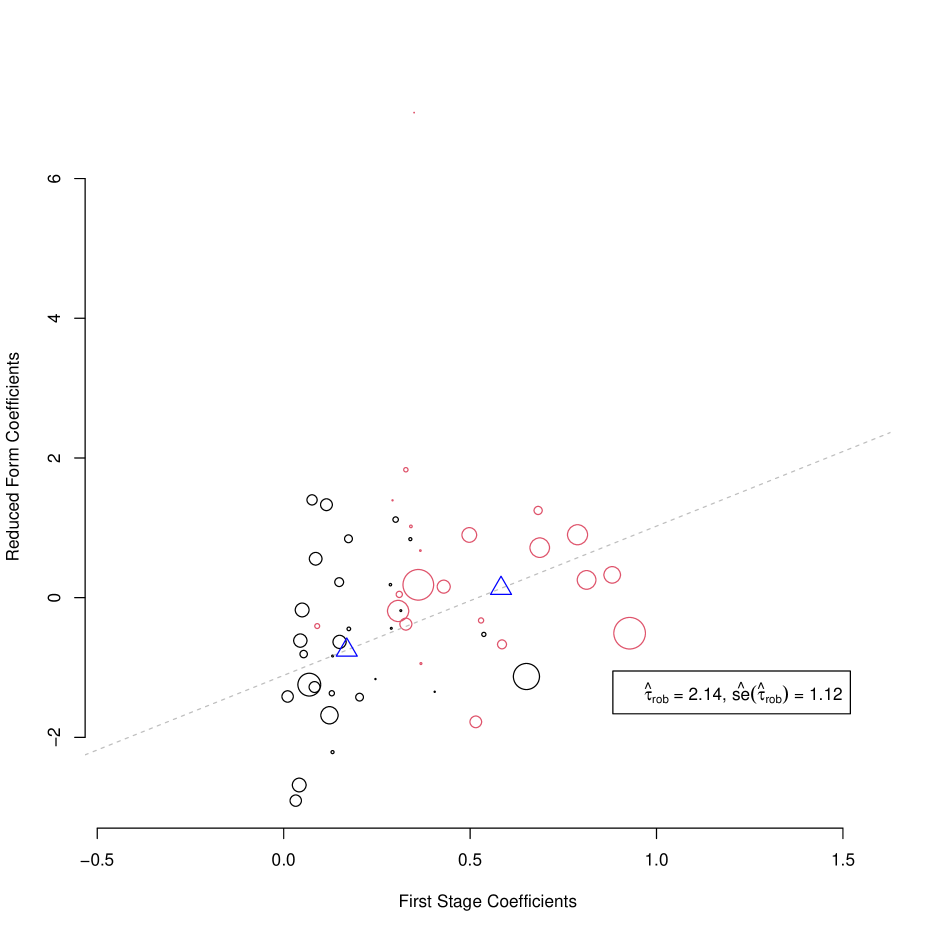
Panel B: Robust weights

Notes: This figure shows the state-level reduced-form and first-stage coefficients for Nakamura and Steinsson (2014) data. Circle sizes reflect the absolute value of weights; negative weights are printed in black, and positive – in red. Blue triangles are centers of mass for negative and positive weights. Panel A presents the results using the whole period of 1968 to 2006 for $n=51$ states. Panel B shows the results from our estimation algorithm. Under our data splitting procedure, Panel B reports the results for 1978-2006, as we use the first $1/3$ of the data for weight estimation.

If we compare $\hat{\tau}_{rob}$ with the estimator that uses the second part of the data but with original weights, they are now different – $2.14$ and $1.83$, respectively. Still, there is a significant difference in estimated standard errors – $45\%$, in favor of the robust estimator. It confirms the intuition from the time-series plots 6, where the aggregate data is much better predicted by $Z_{t}$ if we use robust weights vs. the original ones. The increase in estimated $R^{2}$ is $57\%$ for the endogenous variable and more than $100\%$ for the outcome variable. Figure 7 suggests that these gains come from compressing the distribution of the weights.

Figure 6: Aggregate time-series data for Nakamura and Steinsson (2014) data

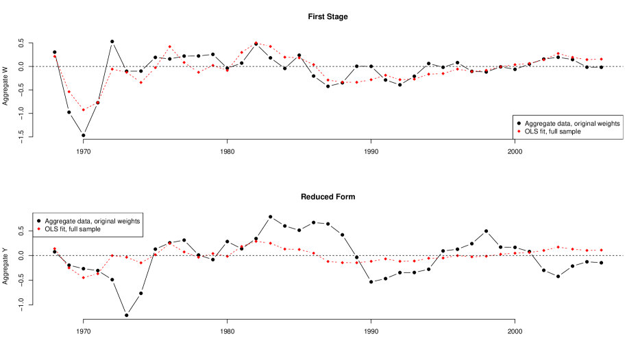
Panel A: Aggregation over $n=51$ states with original weights

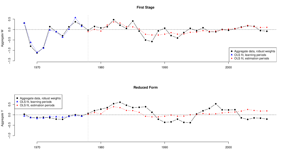
Panel B: Aggregation over $n=51$ states with robust weights

Notes: Solid lines represent aggregate data for different weights; dashed lines represent OLS predictions of the aggregate data with the instrument. The mean absolute value of weights is scaled to $1$.

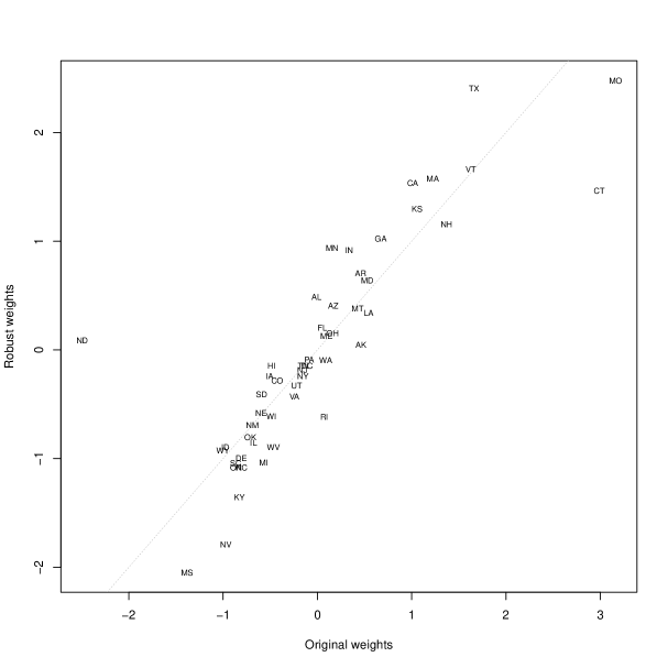
Figure 7: Scatterplot—Nakamura and Steinsson weights and robust weights

Notes: Scatter plot of original and robust weights for Nakamura and Steinsson (2014) data; $n=51$, state abbreviations are used as labels. The variance of weights is scaled to $1$.

Appendix B Proofs

In Sections B.1 - B.3 we prove the results stated in the main text. In Section B.1 we prove Theorems 3.1 - 3.3 taking the results about the robust weights $\omega^{rob}_{i}$ as given. In Section B.2, we consider an abstract quadratic optimization problem and derive properties of its solution. We then establish a connection between abstract stochastic and determinstic optimization problems. In Section B.3, we specialize this connection to the probabilistic models from the main text and prove the results about the robust weights.

We use $\|\cdot\|_{2}$ to denote the euclidean norm, $\|\cdot\|_{\infty}$ to denote the $\sup$-norm, $\|\cdot\|_{HS}$ to denote the Hilbert-Schmidt norm, and $\|\cdot\|_{op}$ – the operator norm. For a random vector $X$ we use $\|X\|_{\psi_{2}}$ to denote its sub-gaussian norm. We use $\textbf{tr}\left(A\right)$ to denote the trace of a square matrix $A$. For a given set of variables $\{X_{i}\}_{i=1}^{n}$ we use $\mathbb{P}_{n}X_{i}$ to denote their average. For any $T\geq T_{b}>T_{a}\geq 1$ we define two projection matrices:

$$\Pi^{f,r}_{T_{a}|T_{b}}=\frac{1}{T_{b}-T_{a}+1}\mathbf{1}_{T_{b}-T_{a}+1}\mathbf{1}_{T_{b}-T_{a}+1}^{\top},\quad\left(\Pi^{f,r}_{T_{a}|T_{b}}\right)^{\bot}=\mathcal{I}_{T_{b}-T_{a}+1}-\Pi^{f,r}_{T_{a}|T_{b}}$$

Also, for any $T>T_{a}>1$ and $k\in\{z,h\}$ we define $\Lambda^{(k),1|T_{a}}_{T_{a}+1|T}$ and $\Lambda^{(k),T_{a}+1|T}_{T_{a}+1|T}$ as submatrices of $\Lambda^{(k)}_{T_{a}+1|T}$ that correspond to shocks from periods $[1,T_{a}]$ and $(T_{a},T]$, respectively. We also define the matrix that project out the time fixed effects:

$$\Pi^{\bot}_{l,f}=\mathcal{I}_{n}-\frac{1}{n}\mathbf{1}_{n}^{\top}\mathbf{1}_{n}.$$

B.1 Part I

B.1.1 Technical lemmas

Lemma B.1.

Let $\Pi_{p}$ be an orthogonal projector on $p$-dimensional subspace or $\mathbb{R}^{T}$ and consider a $T\times n$ matrix $A$ such that $\frac{\|A\|_{op}}{\|A\|_{HS}}=o\left(\frac{1}{\sqrt{p}}\right)$. Then we have

$$\frac{\|(\mathcal{I}_{T}-\Pi)A\|_{HS}}{\|A\|_{HS}}=1+o(1).$$

Proof.

The result follows from a chain of inequalities:

$$\left|\frac{\|(\mathcal{I}_{T}-\Pi)A\|_{HS}}{\|A\|_{HS}}-1\right|\leq\frac{\|\Pi A\|_{HS}}{\|A\|_{HS}}\leq\frac{\|\Pi\|_{HS}\|A\|_{op}}{\|A\|_{HS}}=\sqrt{p}\times o\left(\frac{1}{\sqrt{p}}\right)=o(1).$$

∎

Lemma B.2.

Suppose $\nu^{(z)}$ and $\nu^{(h)}$ are independent, isotropic mean-zero vectors with independent coordinates and subgaussian norms bounded by $1$. Then for any $x<1$ and an absolute constant $c$ we have with probability at least $1-4\exp\left(-cx^{2}\frac{\|B\|^{2}_{HS}}{\|B\|_{op}^{2}}\right)$

$$\left|(\nu^{(z)})AB\nu^{(z)}-\textbf{tr}\left(AB\right)\right|\leq x\frac{\|A\|_{op}\|B\|^{2}_{HS}}{\|B\|_{op}},$$

$$\left|(\nu^{(z)})AB\nu^{(h)}\right|\leq x\frac{\|A\|_{op}\|B\|^{2}_{HS}}{\|B\|_{op}}.$$

Proof.

Proof follows directly from Hanson-Wright inequality and its proof (e.g., Theorem 6.2.1 in Vershynin (2018)). ∎

B.1.2 Theorems in the main text

Proof of Theorem 3.1:

Proof.

We start with the TSLS estimator which under Assumptions 3.1, 3.4 can be represented as

$$\hat{\tau}_{TSLS}-\tau=\frac{\frac{1}{\sqrt{T}}\alpha_{1|T}^{(y)}(\omega^{TSLS})\epsilon^{(z)}+\frac{1}{T}\hat{\rho}(\theta^{(y)},D)\hat{\sigma}(\theta^{(y)})/\hat{\sigma}(D)(\epsilon^{(h)})^{\top}(\Pi^{f,r}_{1|T})^{\bot}\epsilon^{(z)}}{\frac{1}{\sqrt{T}}\alpha_{1|T}^{(w)}(\omega^{TSLS})\epsilon^{(z)}+\frac{1}{T}\hat{\rho}(\theta^{(w)},D)\hat{\sigma}(\theta^{(w)})/\hat{\sigma}(D)(\epsilon^{(h)})^{\top}(\Pi^{f,r}_{1|T})^{\bot}\epsilon^{(z)}+\frac{1}{T}\eta_{\pi}(\epsilon^{(z)})^{\top}(\Pi^{f,r}_{1|T})^{\bot}\epsilon^{(z)}}.$$ (2.1)

We have for $k\in\{y,w\}$

$$\alpha_{1|T}^{(k)}(\omega^{TSLS})\epsilon^{(z)}=\alpha_{1|T}^{(k)}(\omega^{TSLS})\Lambda^{(z)}\nu^{(z)}\Rightarrow\|\alpha_{1|T}^{(k)}(\omega^{TSLS})\epsilon^{(z)}\|_{\psi_{2}}\lesssim\|\alpha_{1|T}^{(k)}(\omega^{TSLS})\Lambda^{(z)}\|_{2}\leq\\ \frac{\|\alpha^{(k)}\|_{op}}{\sqrt{Tn}}\frac{\|\omega^{TSLS}\|_{2}}{\sqrt{n}}\|\Lambda^{(z)}\|_{op}\lesssim 1,$$ (2.2)

where the first implication follows from Assumptions 3.2, 3.3, and the last inequality follows from Assumption 3.6. We next apply Lemma B.2 for $x=\frac{1}{\sqrt{T}}$, and use Assumption 3.3 and Lemma B.1 to get

$$\frac{1}{T}(\epsilon^{(h)})^{\top}(\Pi^{f,r}_{1|T})^{\bot}\epsilon^{(z)}=\rho_{1|T}\sigma_{h,1|T}\sigma_{z,1|T}+O_{p}\left(\frac{1}{\sqrt{T}}\right),$$ (2.3)

$$\frac{1}{T}(\epsilon^{(z)})^{\top}(\Pi^{f,r}_{1|T})^{\bot}\epsilon^{(z)}=\sigma^{2}_{z,1|T}+O_{p}\left(\frac{1}{\sqrt{T}}\right).$$

Using these bounds we get

$$\hat{\tau}_{TSLS}-\tau=\frac{\hat{\rho}_{cs}^{(y)}\hat{\sigma}_{\theta^{(y)}}\rho_{1|T}\sigma_{h,1|T}+O_{p}\left(\frac{1}{\sqrt{T}}\right)}{\hat{\rho}_{cs}^{(w)}\hat{\sigma}_{\theta^{(w)}}\rho_{1|T}\sigma_{h,1|T}+\eta_{\pi}\hat{\sigma}_{D}\sigma_{z,1|T}+O_{p}\left(\frac{1}{\sqrt{T}}\right)}=\frac{\rho_{cs}^{(y)}\sigma_{\theta^{(y)}}\rho_{1|T}\sigma_{h,1|T}+o(1)+O_{p}\left(\frac{1}{\sqrt{T}}\right)}{\rho_{cs}^{(w)}\sigma_{\theta^{(w)}}\rho_{1|T}\sigma_{h,1|T}+\eta_{\pi}\sigma_{D}\sigma_{z,1|T}+o(1)+O_{p}\left(\frac{1}{\sqrt{T}}\right)}$$

and the result for the TSLS follows.

Under Assumptions 3.1, 3.4 we have

$$\hat{\tau}_{rob}-\tau=\\ \frac{\frac{1}{\sqrt{T_{1}}}\alpha_{T_{0}+1|T}^{(y)}(\omega^{rob})\epsilon_{T_{0}+1|T}^{(z)}+\frac{1}{T_{1}}\mathbb{P}_{n}\omega^{rob}_{i}\theta_{i}^{(y)}(\epsilon_{T_{0}+1|T}^{(h)})^{\top}(\Pi^{f,r}_{T_{0}+1|T})^{\bot}\epsilon_{T_{0}+1|T}^{(z)}}{\frac{\alpha_{T_{0}+1|T}^{(w)}(\omega^{rob})\epsilon_{T_{0}+1|T}^{(z)}}{\sqrt{T_{1}}}+\frac{\mathbb{P}_{n}\omega^{rob}_{i}\theta_{i}^{(w)}(\epsilon_{T_{0}+1|T}^{(h)})^{\top}(\Pi^{f,r}_{T_{0}+1|T})^{\bot}\epsilon_{T_{0}+1|T}^{(z)}}{T_{1}}+\frac{\eta_{\pi}(\epsilon_{T_{0}+1|T}^{(z)})^{\top}(\Pi^{f,r}_{T_{0}+1|T})^{\bot}\epsilon_{T_{0}+1|T}^{(z)}}{T_{1}}}$$ (2.4)

Similar to the result above we have:

$$\frac{1}{T_{1}}(\epsilon^{(h)})^{\top}(\Pi^{f,r}_{T_{0}+1|T})^{\bot}\epsilon^{(z)}=\rho_{T_{0}+1|T}\sigma_{h,T_{0}+1|T}\sigma_{z,T_{0}+1|T}+O_{p}\left(\frac{1}{\sqrt{T_{1}}}\right),$$ (2.5)

$$\frac{1}{T_{1}}(\epsilon^{(z)})^{\top}(\Pi^{f,r}_{T_{0}+1|T})^{\bot}\epsilon^{(z)}=\sigma^{2}_{z,T_{0}+1|T}+O_{p}\left(\frac{1}{\sqrt{T_{1}}}\right),$$

and by (2.50) we have

$$\mathbb{P}_{n}\omega^{rob}_{i}\theta_{i}^{(w)}=o_{p}(1),\quad\mathbb{P}_{n}\omega^{rob}_{i}\theta_{i}^{(y)}=o_{p}(1),\quad\frac{\|\omega^{rob}\|_{2}}{\sqrt{n}}=O_{p}(1).$$

By definition $\epsilon_{T_{0}+1|T}^{(z)}=\Lambda^{(z),T_{0}+1|T}_{T_{0}+1|T}\nu_{T_{0}+1|T}^{(z)}+\Lambda^{(z),1|T_{0}}_{T_{0}+1|T}\nu_{1|T_{0}}^{(z)}$, and by concentration for anisotropic vectors we have

$$\|\Lambda^{(z),1|T_{0}}_{T_{0}+1|T}\nu_{1|T_{0}}^{(z)}\|_{2}=\|\Lambda^{(z),1|T_{0}}_{T_{0}+1|T}\|_{HS}+O_{p}\left(\|\Lambda^{(z),1|T_{0}}_{T_{0}+1|T}\|_{op}\right)\leq O_{p}(\|\Lambda^{(z),1|T_{0}}_{T_{0}+1|T}\|_{HS}).$$ (2.6)

Since the weights $\omega^{rob}_{i}$ are independent of $\nu_{T_{0}+1|T}^{(z)}$ by construction, we have for $k\in\{y,w\}$

$$\|\alpha_{T_{0}+1|T}^{(k)}(\omega^{rob})\epsilon_{T_{0}+1|T}^{(z)}\|_{2}\leq\|\alpha_{T_{0}+1|T}^{(k)}(\omega^{rob})\Lambda^{(z),T_{0}+1|T}_{T_{0}+1|T}\nu_{T_{0}+1|T}^{(z)}\|_{2}+\|\alpha_{T_{0}+1|T}^{(k)}(\omega^{rob})\Lambda^{(z),1|T_{0}}_{T_{0}+1|T}\nu_{1|T_{0}}^{(z)}\|_{2}=\\ O_{p}\left(\frac{\|\alpha^{(k)}\|_{op}}{\sqrt{nT_{1}}}\frac{\|\omega^{rob}\|_{2}}{\sqrt{n}}\left(\|\Lambda^{(z),T_{0}+1|T}_{T_{0}+1|T}\|_{op}+\|\Lambda^{(z),1|T_{0}}_{T_{0}+1|T}\|_{HS}\right)\right)=O_{p}(1).$$ (2.7)

The result for $\hat{\tau}^{rob}$ then follows by combining all the bounds. ∎

Proof of Theorem 3.2

Proof.

By (2.51) we have:

$$\mathbb{P}_{n}\omega^{rob}_{i}\theta_{i}^{(w)}=o_{p}\left(\frac{1}{\sqrt{T_{0}}}\right),\quad\mathbb{P}_{n}\omega^{rob}_{i}\theta_{i}^{(y)}=o_{p}\left(\frac{1}{\sqrt{T_{0}}}\right),\quad\frac{1}{\sqrt{n}}\|\omega^{rob}-\omega^{det}_{T_{0}}\|_{2}=o_{p}(1).$$ (2.8)

Using the expansion from the previous theorem we can conclude that the dominant part of the error is coming from $\alpha_{T_{0}+1|T}^{(y)}(\omega^{rob})\epsilon_{T_{0}+1|T}^{(z)}$. We can split this term into two parts:

$$\alpha_{T_{0}+1|T}^{(y)}(\omega^{rob})\epsilon_{T_{0}+1|T}^{(z)}=\alpha_{T_{0}+1|T}^{(y)}(\omega^{rob}-\omega^{det}_{T_{0}})\epsilon_{T_{0}+1|T}^{(z)}+\alpha_{T_{0}+1|T}^{(y)}(\omega^{det}_{T_{0}})\epsilon_{T_{0}+1|T}^{(z)}.$$ (2.9)

By a straightforward extension of the argument in the previous proof we can conclude that the first term is $o_{p}(1)$. Using this we get the following expression:

$$\sqrt{T_{1}}\left(\hat{\tau}_{rob}-\tau\right)=\frac{\left\|\alpha_{T_{0}+1|T}^{(y)}(\omega^{det}_{T_{0}})\Lambda^{(z)}_{T_{0}+1|T}\right\|_{2}}{\eta_{\pi}\sigma^{2}_{z,T_{0}+1|T}}\xi_{n}+o_{p}(1).$$ (2.10)

where $\xi_{n}$ is a sub-gaussian centered random variable with unit variance. To justify normality we use the bound:

$$\frac{\left\|\alpha_{T_{0}+1|T}^{(y)}(\omega^{det}_{T_{0}})\Lambda^{(z)}_{T_{0}+1|T}\right\|_{\infty}}{\left\|\alpha_{T_{0}+1|T}^{(y)}\omega^{det}_{T_{0}})\Lambda^{(z)}_{T_{0}+1|T}\right\|_{2}}\leq\frac{\left\|\left(\Lambda^{(z)}_{T_{0}+1|T}\right)^{\top}\right\|_{\infty}}{\sigma_{\min}}\frac{\left\|\alpha_{T_{0}+1|T}^{(y)}(\omega^{det}_{T_{0}})\right\|_{\infty}}{\left\|\alpha_{T_{0}+1|T}^{(y)}(\omega^{det}_{T_{0}})\right\|_{2}}=o(1),$$ (2.11)

where we used the bound

$$\left\|\alpha_{T_{0}+1|T}^{(y)}(\omega^{det}_{T_{0}})\Lambda^{(z)}_{T_{0}+1|T}\right\|_{2}^{2}=\left\|\alpha_{T_{0}+1|T}^{(y)}(\omega^{det}_{T_{0}})\Lambda^{(z),T_{0}+1|T}_{T_{0}+1|T}\right\|_{2}^{2}+\\ \left\|\alpha_{T_{0}+1|T}^{(y)}(\omega^{det}_{T_{0}})\Lambda^{(z),1|T_{0}}_{T_{0}+1|T}\right\|_{2}^{2}\geq\sigma^{2}_{\min}\|\alpha_{T_{0}+1|T}^{(y)}(\omega^{det}_{T_{0}})\|_{2}^{2}.$$ (2.12)

Using Lindeberg’s CLT we can conclude that $\xi_{n}$ converges in distribution to a standard normal distribution. ∎

Proof of Theorem 3.3

Proof.

The hypothesis of the theorem guarantees that $\sqrt{T_{1}}(\hat{\tau}_{rob}-\tau)$ is asymptotically normal. We thus only need to guarantee that $\hat{\sigma}_{rob}$ is consistent for the asymptotic standard error. Following the steps of the proof of Theorem 3.1 it is straightforward to show that $\hat{\pi}_{rob}$ is consistent for $\eta_{\pi}$. We also have

$$\frac{1}{T_{1}}\sum_{T_{0}<t<T}\left(Z_{t}-\frac{\sum_{T_{0}<l\leq T}Z_{l}}{T_{1}}\right)^{2}=\frac{1}{T_{1}}\left(\Lambda^{(z)}_{T_{0}+1|T}\nu^{(z)}\right)^{\top}\left(\Pi^{f,r}_{T_{0}+1|T}\right)^{\bot}\Lambda^{(z)}_{T_{0}+1|T}\nu^{(z)}=\\ \sigma^{2}_{z,T_{0}+1|T}+o_{p}(1),$$ (2.13)

where the last inequality follows from Lemma B.2 for $x=o(1)$, Lemma B.1, Assumption 3.3, and definition of $\sigma^{2}_{z,T_{0}+1|T}$. Finally, we have the following:

$$\left|\left\|\hat{\alpha}_{T_{0}+1|T}^{(y)}(\omega^{det}_{T_{0}})\hat{\Lambda}^{(z)}_{T_{0}+1|T}\right\|_{2}-\left\|\alpha_{T_{0}+1|T}^{(y)}(\omega^{det}_{T_{0}})\Lambda^{(z)}_{T_{0}+1|T}\right\|_{2}\right|\leq\left\|\alpha_{T_{0}+1|T}^{(y)}(\omega^{det}_{T_{0}})-\hat{\alpha}_{T_{0}+1|T}^{(y)}(\omega^{det}_{T_{0}})\right\|_{2}\left\|\Lambda^{(z)}_{T_{0}+1|T}\right\|_{op}\\ \left(\left\|\alpha_{T_{0}+1|T}^{(y)}(\omega^{det}_{T_{0}})\right\|_{2}+\left\|\alpha_{T_{0}+1|T}^{(y)}(\omega^{det}_{T_{0}})-\hat{\alpha}_{T_{0}+1|T}^{(y)}(\omega^{det}_{T_{0}})\right\|_{2}\right)\|\hat{\Lambda}^{(z)}_{T_{0}+1|T}-\Lambda^{(z)}_{T_{0}+1|T}\|_{op}=\\ O_{p}\left(\left\|\alpha_{T_{0}+1|T}^{(y)}(\omega^{det}_{T_{0}})-\hat{\alpha}_{T_{0}+1|T}^{(y)}(\omega^{det}_{T_{0}})\right\|_{2}\right)+\\ o_{p}\left(\left\|\alpha_{T_{0}+1|T}^{(y)}(\omega^{det}_{T_{0}})\right\|_{2}+\left\|\alpha_{T_{0}+1|T}^{(y)}(\omega^{det}_{T_{0}})-\hat{\alpha}_{T_{0}+1|T}^{(y)}(\omega^{det}_{T_{0}})\right\|_{2}\right)$$ (2.14)

The result holds as long as $\left\|\alpha_{T_{0}+1|T}^{(y)}(\omega^{det}_{T_{0}})\right\|_{2}=O_{p}(1)$ and $\left\|\alpha_{T_{0}+1|T}^{(y)}(\omega^{det}_{T_{0}})-\hat{\alpha}_{T_{0}+1|T}^{(y)}(\omega^{det}_{T_{0}})\right\|_{2}=o_{p}(1)$. The second part follows from consistency of $\hat{\tau}_{rob}$ and (2.50) that guarantees $\mathbb{P}_{n}\omega^{rob}_{i}\theta_{i}^{(y)}=o_{p}(1)$. The first part follows from the consistency of $\omega^{rob}_{i}$ and Assumption 3.6. ∎

Proof of Proposition 1:

Proof.

Consider $\omega_{i}=\epsilon_{i}^{(d)}-\mathbb{P}_{n}\epsilon_{i}^{(d)}$, it does not satisfy the scale constraint, but as we will see, later it does not matter. By concentration for sub-gaussian vectors, we have with probability approaching $1$:

$$\left(\frac{1}{n}\sum_{i\leq n}\omega_{i}\theta_{i}^{(k)}\right)^{2}=\frac{1}{n}|(\epsilon^{(d)})^{\top}\Pi^{\bot}_{l,f}\Theta^{(k)}|^{2}\lesssim\frac{\log(n)}{n}\frac{\|\Pi^{\bot}_{l,f}\Theta^{(k)}\|_{2}^{2}}{n}\lesssim\frac{\log(n)}{n}.$$ (2.15)

Define $\tilde{L}_{1|T_{a}}^{(k)}:=\frac{\Pi^{\bot}_{l,f}L_{1|T_{a}}^{(k)}\left(\Pi^{f,r}_{1|T_{a}}\right)^{\bot}}{\sqrt{nT_{a}}}$ and $\tilde{E}_{1|T_{a}}^{(k)}:=\frac{\Pi^{\bot}_{l,f}E_{1|T_{a}}^{(k)}\left(\Pi^{f,r}_{1|T_{a}}\right)^{\bot}}{\sqrt{nT_{a}}}$; we have

$$\sum_{t\leq T_{a}}\left(\alpha_{t,1|T_{a}}^{(k)}(\omega)\right)^{2}=\frac{1}{n}\left\|\omega^{\top}\tilde{L}_{1|T_{a}}^{(k)}+\omega^{\top}\tilde{E}_{1|T_{a}}^{(k)}\right\|_{2}^{2}\leq\frac{1}{n}\left(\left\|(\epsilon^{(d)})^{\top}\tilde{L}_{1|T_{a}}^{(k)}\right\|_{2}+\left\|(\epsilon^{(d)})^{\top}\tilde{E}_{1|T_{a}}^{(k)}\right\|_{2}\right)^{2}$$ (2.16)

By concentration of anisotropic sub-gaussian vectors, we have with probability approaching one

$$\left|\left\|(\epsilon^{(d)})^{\top}\tilde{L}_{1|T_{a}}^{(k)}\right\|_{2}-\left\|\tilde{L}_{1|T_{a}}^{(k)}\right\|_{HS}\right|\lesssim\sqrt{\log(n)}\left\|\tilde{L}_{1|T_{a}}^{(k)}\right\|_{op}\lesssim\sqrt{\log(n)}$$ (2.17)

By assumption we also have $\left\|\tilde{L}_{1|T_{a}}^{(k)}\right\|_{HS}\lesssim 1$. Similarly, we have conditionally on $E^{(k)}$ with probability approaching one:

$$\left|\left\|(\epsilon^{(d)})^{\top}\tilde{E}_{1|T_{a}}^{(k)}\right\|_{2}-\left\|\tilde{E}_{1|T_{a}}^{(k)}\right\|_{HS}\right|\lesssim\sqrt{\log(n)}\left\|\tilde{E}_{1|T_{a}}^{(k)}\right\|_{op}$$ (2.18)

By concentration of subgaussian random matrices, we have with probability approaching one

$$\left\|\tilde{E}_{1|T_{a}}^{(k)}\right\|_{op}\lesssim\frac{\sqrt{n}}{\sqrt{nT_{a}}}+\frac{\sqrt{T_{a}}}{\sqrt{nT_{a}}}\lesssim 1,$$ (2.19)

and by Hanson-Wright, inequality

$$\left\|\tilde{E}_{1|T_{a}}^{(k)}\right\|_{HS}^{2}=\frac{\textbf{tr}\left(\tilde{\Sigma}_{1|T_{a}}^{(k)}\right)}{T_{a}}+o_{p}(1).$$ (2.20)

It follows that with probability approaching one, we have

$$\sum_{t\leq T_{a}}\left(\alpha_{t,1|T_{a}}^{(k)}(\omega)\right)^{2}\lesssim\frac{\log(n)}{n}.$$ (2.21)

Finally, for the denominator, we have

$$\sigma^{2}_{k,T_{a}}\geq\left\|\tilde{L}_{1|T_{a}}^{(k)}+\tilde{E}_{1|T_{a}}^{(k)}\right\|_{HS}^{2}=\|\tilde{L}_{1|T_{a}}^{(k)}\|_{HS}+\|\tilde{E}_{1|T_{a}}^{(k)}\|_{HS}^{2}+2\textbf{tr}\left(\left(\tilde{E}_{1|T_{a}}^{(k)}\right)^{\top}\tilde{L}_{1|T_{a}}^{(k)}\right)\geq\\ \frac{\textbf{tr}\left(\tilde{\Sigma}_{1|T_{a}}^{(k)}\right)}{T_{a}}+o_{p}(1).$$ (2.22)

Combining all the bounds and using the fact that $\frac{1}{n}\sum_{i\leq n}D_{i}\omega_{i}=\sigma^{2}_{d}+o_{p}(1)$ we get the result. ∎

Proof of Proposition 2:

Proof.

The proof follows the same steps for Proposition 2 and is omitted. ∎

B.2 Part II

B.2.1 Balancing bounds for quadratic problems

For arbitrary matrices $\{L_{k}\}_{k=1}^{K}$ and vector $c$ consider

$$x_{0}:= \arg\min_{x}\left\{\sum_{k=1}^{K}\|L_{k}x\|_{2}^{2}+\zeta^{2}\|x\|_{2}^{2}\right\},$$ (2.23)

subject to: $$c^{\top}x=1,$$

and let $V^{2}(\zeta^{2})$ be the optimal value of this program. Our goal is to upper bound $\|L_{k}x_{0}\|_{2}$, which can be interpreted as a measure of imbalance. A trivial bound is $\|L_{k}x_{0}\|_{2}\leq V(\zeta^{2})$, and our goal is to establish a better bound under additional conditions on matrices $L_{k}$.

Consider a related program

$$\{\beta_{k,0}\}_{k=1}^{K}:=\arg\min_{\{\beta_{k}\}_{k=1}^{K}}\left\{\left\|c-\sum_{k=1}^{K}L_{k}^{\top}\beta_{k}\right\|_{2}^{2}+\zeta^{2}\sum_{k=1}^{K}\|\beta_{k}\|_{2}^{2}\right\},$$ (2.24)

next lemma describes the balancing properties of $x_{0}$ in terms of $\{\beta_{0,k}\}_{k=1}^{K}$ and $V^{2}(\zeta^{2})$.

Lemma B.3.

Suppose $\|c\|_{2}\neq 0$, then for any $k$ we have

$$\|L_{k}x_{0}\|_{2}=V^{2}(\zeta^{2})\|\beta_{k,0}\|_{2}.$$ (2.25)

Proof.

Using duality (constraint qualification holds because $\|c\|\neq 0$) we have

$$V^{2}(\zeta^{2}):=\min_{x:c^{\top}x=1}\left\{\sum_{k=1}^{K}\|L_{k}x\|_{2}^{2}+\zeta^{2}\|x\|_{2}^{2}\right\}=\\ \min_{x,\{t_{k}\}_{k=1}^{K}}\max_{\lambda_{k}\geq 0,\mu}\left\{\sum_{k=1}^{K}\lambda_{k}(\|L_{k}x\|_{2}-t_{k})+\sum_{k=1}^{K}t_{k}^{2}+\zeta^{2}\|x\|_{2}^{2}+\mu(1-c^{\top}x)\right\}=\\ \min_{x,\{t_{k}\}_{k=1}^{K}}\max_{\|\beta_{k}\|_{2}\leq 1,\lambda_{k}\geq 0,\mu}\left\{\sum_{k=1}^{K}\lambda_{k}(\beta_{k}^{\top}L_{k}x-t_{k})+\sum_{k=1}^{K}t_{k}^{2}+\zeta^{2}\|x\|_{2}^{2}+\mu(1-c^{\top}x)\right\}=$$

$$=\max_{\|\beta_{k}\|_{2}\leq 1,\lambda_{k}\geq 0,\mu}\min_{x,\{t_{k}\}_{k=1}^{K}}\left\{\sum_{k=1}^{K}\lambda_{k}(\beta_{k}^{\top}L_{k}x-t_{k})+\sum_{k=1}^{K}t_{k}^{2}+\zeta^{2}\|x\|_{2}^{2}+\mu(1-c^{\top}x)\right\}=\\ \max_{\beta_{k},\mu}\left\{-\frac{\mu^{2}}{4\zeta^{2}}\left\|c^{\top}-\sum_{k=1}^{K}\beta_{k}^{\top}L_{k}\right\|_{2}^{2}-\frac{\mu^{2}}{4}\left(\sum_{k=1}^{K}\|\beta_{k}\|_{2}^{2}\right)+\mu\right\}=\\ \max_{\beta_{k}}\left\{\frac{\zeta^{2}}{\left\|c-\sum_{k=1}^{K}L_{k}^{\top}\beta_{k}\right\|_{2}^{2}+\zeta^{2}\left(\sum_{k=1}^{K}\|\beta_{k}\|_{2}^{2}\right)}.\right\}$$

We can express $x_{0}$ in terms of the solution to the dual problem:

$$x_{0}=\frac{\left(c-\sum_{k=1}^{K}L_{k}^{\top}\beta_{k,0}\right)}{\left\|c-\sum_{k=1}^{K}L_{k}^{\top}\beta_{k,0}\right\|_{2}^{2}+\zeta^{2}\left(\sum_{k=1}^{K}\|\beta_{k,0}\|_{2}^{2}\right)}.$$

Using the first-order conditions for the dual problem, we have the following for any $k$:

$$\left(c-\sum_{k=1}^{K}L_{k}^{\top}\beta_{k,0}\right)^{\top}L_{k}^{\top}=\zeta^{2}\beta_{k,0}^{\top}\Rightarrow\|L_{k}x_{0}\|_{2}=V^{2}(\zeta^{2})\|\beta_{k,0}\|_{2},$$

where for the implication, we used the relationship between $x_{0}$ and $\beta_{0}$. ∎

By construction, program (2.24) is invariant to the left rotation of $L_{k}$ (the $l_{2}$ norm of coefficients does not change). By virtue of the SVD decomposition, we can, without loss of generality, assume that each $L_{k}$ is a product of two matrices,

$$L_{k}^{\top}=U_{k}D_{k},$$

where each $D_{k}$ is a diagonal matrix of size $p_{k}=\text{rank}(L_{k})$, with positive values on the diagonal, and $U_{k}^{\top}U_{k}=\mathcal{I}_{p_{k}}$. For a given $k$ let $s_{k}\in\mathbb{R}^{p_{k}}$ be a unit vector and define $U(s_{k}):=U_{k}D_{k}s_{k}$, $\sigma(s_{k}):=\|U(s_{k})\|_{2}$, $u(s_{k}):=\frac{1}{\sigma(s_{k})}U(s_{k})$. Fix $k$ and observe that (2.24) is equivalent to the following one:

$$\left(\{\beta_{0,l}\}_{l\neq k},s_{0,k},\lambda_{0,k}\right)=\arg\min_{\{\beta_{l}\}_{l\neq k},s_{k},\lambda_{k}}\left\|c-\sum_{l\neq k}L_{l}^{\top}\beta_{l}-u(s_{k})\sigma(s_{k})\lambda_{k}\right\|_{2}^{2}+\zeta^{2}\left(\sum_{l\neq k}\|\beta_{l}\|_{2}^{2}+\lambda_{k}^{2}\right),$$

where $\beta_{0,k}=\lambda s_{0,k}$ and $\|\beta_{0,k}\|_{2}=|\lambda_{0,k}|$. For fixed $k$, $s_{k}$ and $\zeta^{2}$ define

$$V^{2}(s_{k},\zeta^{2}):=\min_{x:u(s_{k})^{\top}x=1}\left\{\sum_{l\neq k}\|L_{k}x\|_{2}^{2}+\zeta^{2}\|x\|_{2}^{2}\right\},$$

and let $x^{\star}(u(s_{0,k}))$ be the solution to this problem. Next lemma connects $\|\beta_{0,k}\|_{2}$ to $V^{2}(s_{0,k},\zeta^{2})$, $\zeta^{2}$, and $\sigma(s_{0,k})$.

Lemma B.4.

Suppose $\|c\|_{2}\neq 0$, then the following bound is satisfied for all $k$ such that $p_{k}>0$:

$$\|\beta_{0,k}\|_{2}\leq\|c\|_{2}\times\|x^{\star}(u(s_{0,k}))\|_{2}\times\frac{\sigma(s_{0,k})}{V^{2}(s_{0,k},\zeta^{2})+\sigma^{2}(s_{0,k})}.$$ (2.26)

Proof.

Fix $k$ with $p_{k}>0$ and stack matrices $\{L_{l}\}_{l\neq k}$ into a large matrix $L^{\top}_{-k}$, and define $p_{-k}:=\sum_{l\neq k}p_{k}$. Using inversion for block matrices we get the expression for $\lambda_{0,k}$:

$$\lambda_{0,k}=\frac{c^{\top}\tilde{U}(s_{0,k})}{U^{\top}(s_{0,k})\tilde{U}(s_{0,k})+\zeta^{2}},$$

$$\tilde{U}(s_{0,k})=U(s_{0,k})-L_{-k}^{\top}(L_{-k}L_{-k}^{\top}+\zeta^{2}\mathcal{I}_{p_{-k}})^{-1}L_{-k}U(s_{0,k}).$$

Define $\tilde{u}(s_{0,k}):=\frac{1}{\sigma(s_{0,k})}\tilde{U}(s_{0,k})$. We have

$$\left(\tilde{U}(s_{0,k})\right)^{\top}U(s_{0,k})=\sigma^{2}(s_{0,k})\left(\|\tilde{u}(s_{0,k})\|_{2}^{2}+\zeta^{2}\sum_{l\neq k}\|\gamma_{0,l}(s_{0,k})\|_{2}^{2}\right)>0,$$

where $\{\gamma_{0,l}(s_{0,k})\}_{l\neq k}$ is the solution for the optimization problem:

$$\{\gamma_{0,l}(s_{0,k})\}_{l\neq k}=\arg\max_{\{\gamma_{l}\}_{l\neq k}}\left\{\frac{\zeta^{2}}{\|u(s_{0,k})-\sum_{l\neq k}L_{l}^{\top}\gamma_{l}\|_{2}^{2}+\zeta^{2}\sum_{l\neq k}\|\gamma_{l}\|_{2}^{2}}\right\}$$

By the same argument as in Lemma B.3, we have equality between two problems:

$$\max_{\{\gamma_{l}\}_{l\neq k}}\left\{\frac{\zeta^{2}}{\|u(s_{0,k})-\sum_{l\neq k}L_{l}^{\top}\gamma_{l}\|_{2}^{2}+\zeta^{2}\sum_{l\neq k}\|\gamma_{l}\|_{2}^{2}}\right\}=\min_{x:u(s_{0,k})^{\top}x=1}\left\{\sum_{l\neq k}\|L_{k}x\|_{2}^{2}+\zeta^{2}\|x\|_{2}^{2}\right\}.$$

Using Lemma B.3 we get $\|\tilde{u}(s_{0,k})\|_{2}=\frac{\zeta^{2}\|x^{\star}(u(s_{0,k}))\|_{2}}{V^{2}(s_{0,k},\zeta^{2})}$. Combining this result with definition of $\lambda_{0,k}$ we get the bound

$$|\lambda_{0,k}|\leq\frac{\|c\|_{2}\sigma(s_{0,k})\|\tilde{u}(s_{0,k})\|_{2}}{\zeta^{2}+\sigma^{2}(s_{0,k})\frac{\zeta^{2}}{V^{2}(s_{0,k},\zeta^{2})}}\leq\|c\|_{2}\times\|x^{\star}(u(s_{0,k}))\|_{2}\times\frac{\sigma(s_{0,k})}{V^{2}(s_{0,k},\zeta^{2})+\sigma^{2}(s_{0,k})},$$

where we used the CS inequality. Since $|\lambda_{0,k}|=\|\beta_{k}\|_{2}$ we get the result. ∎

Next corollary combines the bounds from Lemmas B.3, B.4.

Corollary B.1.

Suppose $\|c\|_{2}\neq 0$, $V^{2}(s_{0,k},\zeta^{2})\lesssim\zeta^{2}$, $V^{2}(\zeta^{2})\lesssim V^{2}(s_{0,k},\zeta^{2})$, and $\|c\|_{2}\lesssim 1$. Then the following holds for all $k$ such that $p_{k}>0$:

$$\|L_{k}x_{0}\|_{2}\lesssim\min\left\{\frac{\zeta^{2}}{\sigma(s_{0,k})},\sigma(s_{0,k})\right\}.$$ (2.27)

Proof.

Combining the bounds (2.25), (2.26) we have the following for all $k$:

$$\|L_{k}x_{0}\|_{2}\leq V^{2}(\zeta^{2})\|\beta_{k,0}\|_{2}\lesssim\frac{V^{2}(s_{0,k},\zeta^{2})\sigma(s_{0,k})}{V^{2}(s_{0,k},\zeta^{2})+\sigma^{2}(s_{0,k})}\lesssim\min\left\{\frac{\zeta^{2}}{\sigma(s_{0,k})},\sigma(s_{0,k})\right\}.$$

∎

B.2.2 Oracle bound

This section establishes a connection between a random and a deterministic optimization problem. Consider a $T\times n$ matrix $L$ with a special structure:

$$L=H\Theta+\tilde{L},\quad\mathbb{E}[H]=0,$$

where a $k\times n$ matrix $\Theta$ and $T\times n$ matrix $\tilde{L}$ are deterministic. Let $Z$ be a random $T\times p$ matrix, define a random variable

$$\mu^{2}=\frac{\min_{\Phi}\mathbb{E}_{H,Z}\|L-Z\Phi\|^{2}_{HS}}{\min_{\Phi}\|L-Z\Phi\|^{2}_{HS}},$$

where $\Phi$ is a $p\times n$ matrix. Let $A\subseteq\mathbb{R}^{n}$ be a convex set, define solutions to two programs

$$x_{1}:=\arg\min_{x\in A,\psi\in\mathbb{R}^{p}}\Big{\{}\mu^{2}\|Lx-Z\psi\|_{2}^{2}+\zeta^{2}\|x\|_{2}^{2}\Big{\}},$$ (2.28)

$$x_{0}:=\arg\min_{x\in A,\psi\in\mathbb{R}^{p}}\Big{\{}\mathbb{E}_{H,Z}\left[\|Lx-Z\psi\|_{2}^{2}\right]+\zeta^{2}\|x\|_{2}^{2}\Big{\}},$$

and define $\delta:=x_{1}-x_{0}$.

Define projection matrices $\Pi:=Z\left(Z^{\top}Z\right)^{-1}Z^{\top}$ and $\Pi^{\bot}:=\mathcal{I}_{T}-\Pi$. By construction, we have:

$$\min_{\psi\in\mathbb{R}^{p}}\|Lx-Z\psi\|_{2}^{2}=\|\Pi^{\bot}Lx\|_{2}^{2},$$

and can re-express $x_{1}$ differently:

$$x_{1}:=\arg\min_{x\in A}\Big{\{}\mu^{2}\|\Pi^{\bot}Lx\|_{2}^{2}+\zeta^{2}\|x\|_{2}^{2}\Big{\}}.$$

Using the definition of $L$ we expand the expectation:

$$\mathbb{E}_{H,Z}\left[\|Lx-Z\psi\|_{2}^{2}\right]=\|\tilde{L}x\|_{2}^{2}+\mathbb{E}_{H,Z}\left[\|H\Theta x-Z\psi\|_{2}^{2}\right].$$

The minimum value of the second part can be expressed differently:

$$\min_{\psi\in\mathbb{R}^{p}}\mathbb{E}_{H,Z}\left[\|H\Theta x-Z\psi\|_{2}^{2}\right]=x^{\top}\Theta^{\top}\mathbb{E}_{H,Z}[(H-Z\Psi^{\star})^{\top}(H-Z\Psi^{\star})]\Theta x,$$

where $\Psi^{\star}=\left(\mathbb{E}_{H,Z}[Z^{\top}Z]\right)^{-1}\mathbb{E}_{H,Z}[Z^{\top}H]$. Similarly for $\hat{\Psi}=\left(Z^{\top}Z\right)^{-1}\left(Z^{\top}H\right)$ we can express the empirical value:

$$\min_{\psi\in\mathbb{R}^{p}}\|H\Theta x-Z\psi\|_{2}^{2}=x^{\top}\Theta^{\top}(H-Z\hat{\Psi})^{\top}(H-Z\hat{\Psi})\Theta x.$$

Define two matrices

$$K:=\mathbb{E}[(H-Z\Psi^{\star})^{\top}(H-Z\Psi^{\star})],\quad\hat{K}:=(H-Z\hat{\Psi})^{\top}(H-Z\hat{\Psi}).$$ (2.29)

and suppose that a symmetric matrix $K$ is invertible. Define a relative distance between $\hat{K}$ and $K$:

$$E:=K^{-\frac{1}{2}}(K-\hat{K})K^{-\frac{1}{2}}=\mathcal{I}_{k}-K^{-\frac{1}{2}}\hat{K}K^{-\frac{1}{2}},$$

and several quantities that govern the behavior of the bound later:

$$\xi_{1}^{2}:=\frac{\|\Pi\tilde{L}\delta\|_{2}^{2}}{\|\delta\|_{2}^{2}},\quad\xi_{2}:=\frac{|x_{0}^{\top}\tilde{L}^{\top}\Pi\tilde{L}\delta|}{\|\tilde{L}\delta\|_{2}\|\tilde{L}x_{0}\|_{2}},\quad\xi_{3}:=\frac{|x_{0}^{\top}\Theta^{\top}H\Pi^{\bot}\tilde{L}\delta|}{\|K^{\frac{1}{2}}\Theta x_{0}\|_{2}\|\tilde{L}\delta\|_{2}},$$

$$\xi_{4}:=\frac{|x_{0}^{\top}\tilde{L}^{\top}\Pi^{\bot}H^{\top}\Theta\delta|}{\|K^{\frac{1}{2}}\Theta\delta\|_{2}\|\tilde{L}x_{0}\|_{2}},\quad\xi_{5}:=\frac{|x_{0}^{\top}\Theta^{\top}H^{\top}\Pi^{\bot}H\Theta\delta|}{\|K^{\frac{1}{2}}\Theta x_{0}\|_{2}\|K^{\frac{1}{2}}\Theta\delta\|_{2}}.$$

Define a set $A_{1}$ on which three inequalities hold:

$$\|E\|_{op}\leq\frac{1}{2},\quad\|\Pi^{\bot}L\delta\|_{2}^{2}\geq\frac{1}{2}\left(\|\Pi^{\bot}H\Theta\delta\|_{2}^{2}+\|\Pi^{\bot}\tilde{L}\delta\|_{2}^{2}\right),\quad|\mu^{2}-1|\leq\frac{1}{4}.$$

In addition, define a set $A_{2}$ on which another inequality holds:

$$\zeta^{2}\geq\xi_{1}^{2}.$$

Next lemma provides a connection between two programs (2.28).

Lemma B.5.

Suppose matrix $K$ is invertible, then on $A_{1}\cap A_{2}$ we have the following bounds:

$$\|K^{\frac{1}{2}}\Theta\delta\|_{2}\lesssim(\|\hat{E}\|_{op}+\xi_{3}+|\mu^{2}-1|\xi_{5})\|K^{\frac{1}{2}}\Theta x_{0}\|_{2}+(\xi_{4}+\xi_{2}+|\mu^{2}-1|)\|\tilde{L}x_{0}\|_{2},$$ (2.30)

$$\|\tilde{L}\delta\|_{2}\lesssim(\|\hat{E}\|_{op}+\xi_{3}+|\mu^{2}-1|\xi_{5})\|K^{\frac{1}{2}}\Theta x_{0}\|_{2}+(\xi_{4}+\xi_{2}+|\mu^{2}-1|)\|\tilde{L}x_{0}\|_{2},$$

$$\|\delta\|_{2}\lesssim\frac{(\|\hat{E}\|_{op}+\xi_{3}+|\mu^{2}-1|\xi_{5})\|K^{\frac{1}{2}}\Theta x_{0}\|_{2}+(\xi_{4}+\xi_{2}+|\mu^{2}-1|)\|\tilde{L}x_{0}\|_{2}}{\zeta}.$$

Proof.

Using first order conditions for (2.28) we have two inequalities:

$$\mu^{2}x_{1}^{\top}L^{\top}\Pi^{\bot}L\delta+\zeta^{2}x_{1}^{\top}\delta\leq 0,\quad x_{0}^{\top}K\delta+x_{0}^{\top}\tilde{L}^{\top}\tilde{L}\delta+\zeta^{2}x_{0}^{\top}\delta\geq 0.$$

Combining these inequalities, we get:

$$\mu^{2}\|\Pi^{\bot}L\delta\|_{2}^{2}+\zeta^{2}\|\delta\|_{2}^{2}+x_{0}^{\top}\Theta^{\top}(\hat{K}-K)\Theta^{\top}\delta-x_{0}^{\top}\tilde{L}^{\top}\Pi\tilde{L}\delta+\mu^{2}x_{0}^{\top}\Theta^{\top}H\Pi^{\bot}\tilde{L}\delta+\mu^{2}x_{0}^{\top}\tilde{L}^{\top}\Pi^{\bot}H\Theta\delta+\\ (\mu^{2}-1)x_{0}^{\top}\tilde{L}^{\top}\Pi^{\bot}\tilde{L}\delta+(\mu^{2}-1)x_{0}^{\top}\Theta^{\top}H^{\top}\Pi^{\bot}H\Theta\delta\leq 0.$$

By CS we have

$$\left|(\mu^{2}-1)x_{0}^{\top}\tilde{L}^{\top}\Pi^{\bot}\tilde{L}\delta\right|\leq|\mu^{2}-1|\|\tilde{L}x_{0}\|_{2}\|\tilde{L}\delta\|_{2},$$

$$\left|(\mu^{2}-1)x_{0}^{\top}\Theta^{\top}H^{\top}\Pi^{\bot}H\Theta\delta\right|\leq\xi_{5}|\mu^{2}-1|\|K^{\frac{1}{2}}\Theta x_{0}\|_{2}\|K^{\frac{1}{2}}\Theta\delta\|_{2}.$$

By definition using the fact that $K$ is invertible:

$$\|\Pi^{\bot}H\Theta\delta\|_{2}^{2}=\left(\Theta\delta\right)^{\top}K\Theta\delta+\left(\Theta\delta\right)^{\top}K^{\frac{1}{2}}\hat{E}K^{\frac{1}{2}}\Theta\delta\geq\|K^{\frac{1}{2}}\Theta\delta\|_{2}^{2}(1-\|\hat{E}\|_{op}),$$

$$x_{0}^{\top}\Theta^{\top}(\hat{K}-K)\Theta^{\top}\delta\geq-\|K^{\frac{1}{2}}\Theta x_{0}\|_{2}\|\hat{E}\|_{op}\|K^{\frac{1}{2}}\Theta^{\top}\delta\|_{2}.$$

By the properties of the projection matrix and definition of $\xi_{1}^{2}$:

$$\|\Pi^{\bot}\tilde{L}\delta\|_{2}^{2}=\|\tilde{L}\delta\|_{2}^{2}-\|\Pi\tilde{L}\delta\|_{2}^{2}=\|\tilde{L}\delta\|_{2}^{2}-\xi_{1}^{2}\|\delta\|_{2}^{2}.$$

Combining these results, definitions of $\xi_{2},\xi_{3},\xi_{4}$ we have the following on $A_{1}\cap A_{2}$:

$$0\geq\frac{3}{16}\|K^{\frac{1}{2}}\Theta\delta\|_{2}^{2}+\frac{3}{8}\|\tilde{L}\delta\|_{2}^{2}+\frac{3}{8}\zeta^{2}\|\delta\|_{2}^{2}-\left(\|K^{\frac{1}{2}}\Theta x_{0}\|_{2}\left(\|\hat{E}\|_{op}+|\mu^{2}-1|\xi_{5}\right)+\xi_{4}\|\tilde{L}x_{0}\|_{2}\right)\|K^{\frac{1}{2}}\Theta^{\top}\delta\|_{2}-\\ \left(\|K^{\frac{1}{2}}\Theta x_{0}\|_{2}\xi_{3}+(\xi_{2}+|\mu^{2}-1|)\|\tilde{L}x_{0}\|_{2}\right)\|\tilde{L}\delta\|_{2}.$$

This expression has the following form (for appropriate $x_{1},x_{2},x_{3},a_{1},a_{2}$):

$$0\geq x_{1}^{2}+x_{2}^{2}+x_{3}^{2}-2a_{1}x_{1}-2a_{2}x_{2}=(x_{1}-a_{1})^{2}+(x_{2}-a_{2})^{2}+x_{3}^{2}-a_{1}^{2}-a_{2}^{2}\Rightarrow\\ \begin{cases}x_{1}\leq a_{1}+\sqrt{a_{1}^{2}+a_{2}^{2}}\\ x_{2}\leq a_{2}+\sqrt{a_{1}^{2}+a_{2}^{2}}\\ x_{3}\leq\sqrt{a_{1}^{2}+a_{2}^{2}}.\end{cases}\Rightarrow\begin{cases}x_{1}\lesssim a_{1}+a_{2}\\ x_{2}\lesssim a_{1}+a_{2}\\ x_{3}\lesssim a_{1}+a_{2}.\end{cases}$$

Substituting $x_{1},x_{2},x_{3}$ and $a_{1},a_{2}$ we get the result. ∎

B.3 Part III

Lemma B.5 and Corollary B.1 allow us to connect the empirical problem to a deterministic program for which we have a general bound. These results do not restrict the dimension of $H$ as long as their assumptions are satisfied. In particular, we need to guarantee that the hypothesis of Lemma B.5 holds with high probability and establish high-probability bounds on $\xi_{1},\dots,\xi_{5}$. These guarantees can be established under different assumptions on $H$, and below we prove them for the one-dimensional and sub-gaussian case. As long as the dimension of $H$ remains bounded one can establish similar rates at the cost of more elaborate notation.

B.3.1 One-dimensional subgaussian noise

In this section, we analyze the bounds from the previous section under additional assumptions on $H$ and $Z$.

Assumption B.1.

Suppose $L=H\Theta+\tilde{L}$, where

$$H=\Lambda_{h}\nu d_{h},\quad Z=\Lambda_{z}\nu d_{z},$$

and $d_{h}=(1,0)$, $d_{z}=(\rho,\sqrt{1-\rho^{2}})$, $\nu$ is a $T\times 2$ matrix, and $\Lambda_{h}$, $\Lambda_{z}$ are $T\times T$ matrices.

Our goal is to lower bound the probabilities of sets $A_{1},A_{2}$ and bound $\xi_{1}^{2},\xi_{2},\xi_{3},\xi_{4},\xi_{5}$ under the tail assumptions on $\nu$, restrictions on $\Lambda_{h},\Lambda_{z}$, and $\rho$. All asymptotic statements in this section are with respect to $T$ going to infinity.

Assumption B.2.

Random variables $\nu_{tk}=(\nu)_{(t,k)}$ are i.i.d. across $t$ and $k$, and $\|\nu_{t,k}\|_{\psi^{2}}\lesssim\mathbb{E}[\nu_{t,k}^{2}]>0$.

Assumption B.3.

$|\rho|<c_{\rho}<1$, $\|\Lambda_{z}\|_{op}\sim\|\Lambda_{h}\|_{op}$, $\|\Lambda_{h}\|_{HS}\sim\|\Lambda_{z}\|_{HS}$, $\|\Lambda_{h}\|_{op}=o\left(\|\Lambda_{h}\|_{HS}\right)$.

Next lemma established properties of $K$ define in (2.29).

Lemma B.6.

Suppose Assumptions B.1, B.2, B.3 hold, then $K=\left(1-\rho^{2}\frac{\left(\textbf{tr}\left(\Lambda_{h}^{\top}\Lambda_{z}\right)\right)^{2}}{\|\Lambda_{z}\|_{HS}^{2}\|\Lambda_{h}\|_{HS}^{2}}\right)\mathbb{E}[\nu_{tk}^{2}]\|\Lambda_{h}\|_{HS}^{2}>0$.

Proof.

Result follows from definition of $K$:

$$K=\mathbb{E}[\|H\|_{2}^{2}]-\frac{\mathbb{E}[H^{\top}Z]^{2}}{\left(\mathbb{E}[\|Z\|_{2}^{2}]\right)^{2}}\mathbb{E}[\|Z\|_{2}^{2}]=\mathbb{E}[\|H\|_{2}^{2}]\left(1-\frac{\mathbb{E}[H^{\top}Z]^{2}}{\mathbb{E}[\|Z\|_{2}^{2}]\mathbb{E}[\|H\|_{2}^{2}]}\right),$$

and Assumptions B.1, B.2, B.3. ∎

Lemma B.7.

Suppose that Assumptions B.1, B.2, B.3 hold, and $\mathbb{E}[\nu_{tk}^{2}]=1$. Suppose $\max\{x_{1},x_{3}\}\lesssim\frac{\|\Lambda_{h}\|_{HS}}{\|\Lambda_{h}\|_{op}}$, $x_{2}\lesssim\frac{\|\Lambda_{z}\|_{HS}}{\|\Lambda_{z}\|_{op}}$. Then with probability at least $1-c\exp(-cx_{1}^{2})-c\exp(-cx_{2}^{2})-c\exp(-cx_{3}^{2})$ we have

$$\frac{|\|H\|_{2}^{2}-\|\Lambda_{h}\|_{HS}^{2}|}{\|\Lambda_{h}\|_{HS}^{2}}\leq x_{1}\frac{\|\Lambda_{h}\|_{op}}{\|\Lambda_{h}\|_{HS}},\quad\frac{|\|Z\|_{2}^{2}-\|\Lambda_{z}\|_{HS}^{2}|}{\|\Lambda_{z}\|_{HS}^{2}}\leq x_{2}\frac{\|\Lambda_{z}\|_{op}}{\|\Lambda_{z}\|_{HS}},$$ (2.31)

$$\frac{|Z^{\top}H-\rho\textbf{tr}\left(\Lambda_{z}^{\top}\Lambda_{h}\right)|}{\|\Lambda_{h}\|_{HS}^{2}}\leq x_{3}(|\rho|+\sqrt{1-\rho^{2}})\frac{\|\Lambda_{h}\|_{op}}{\|\Lambda_{h}\|_{HS}}.$$

Proof.

We focus only on the first inequality, the second follows in the same way. By Hanson-Wright inequality the inequality holds with probability at least

$$1-2\exp\left(-c\min\left\{x_{1}\frac{\|\Lambda_{h}\|_{op}}{\|\Lambda_{h}\|_{HS}},x_{1}^{2}\left(\frac{\|\Lambda_{h}\|_{op}}{\|\Lambda_{h}\|_{HS}}\right)^{2}\right\}\frac{\|\Lambda_{h}\|_{HS}^{2}}{\|\Lambda_{h}\|_{op}^{2}}\right)=1-2\exp(-cx_{1}^{2}),$$

where the second equality follows from Assumptions on $x_{1}$. To analyze the last quantity we split it into two using Assumption B.1:

$$|Z^{\top}H-\rho\textbf{tr}\left(\Lambda_{z}^{\top}\Lambda_{h}\right)|=|\rho||d_{h}\nu^{\top}\Lambda_{z}^{\top}\Lambda_{h}\nu d_{h}-\textbf{tr}\left(\Lambda_{z}^{\top}\Lambda_{h}\right)|+\sqrt{1-\rho^{2}}|\nu_{(1)}^{\top}\Lambda_{z}^{\top}\Lambda_{h}\nu_{(2)}|$$

For the first quantity we can use Hanson-Wright inequality as before, utilizing Assumption B.3. For the second one we can use the argument from Vershynin (2018) Theorem 6.2.1 to make the same conclusion. ∎

Define the empirical regression coefficient $\hat{\psi}=\frac{H^{\top}Z}{\|Z\|_{2}^{2}}$, and its population counterpart $\psi=\frac{\rho\textbf{tr}\left(\Lambda_{z}^{\top}\Lambda_{h}\right)}{\|\Lambda_{z}\|_{HS}^{2}}$. Next corollary quantifies the error of $\hat{\psi}$.

Corollary B.2.

Suppose Assumptions B.1, B.2, B.3 hold, then for any $x\lesssim\frac{\|\Lambda_{z}\|_{HS}}{\|\Lambda_{z}\|_{op}}$

$$|\hat{\psi}-\psi|\leq x\frac{\|\Lambda_{z}\|_{op}}{\|\Lambda_{z}\|_{HS}}$$ (2.32)

holds with probability at least $1-c\exp(-cx^{2})$. In particular, $\hat{\psi}$ is consistent.

Proof.

By construction $\hat{\psi}$ is scale invariant with respect to $\nu$ so we can assume $\mathbb{E}[\nu_{tk}^{2}]=1$. The result then follows from applying Lemma B.7 together with the following expansion:

$$\hat{\psi}-\psi=\frac{Z^{\top}H}{\|Z\|_{2}^{2}}-\psi=\frac{1}{\|\Lambda_{z}\|_{HS}^{2}}\frac{Z^{\top}H-\rho\textbf{tr}\left(\Lambda_{z}^{\top}\Lambda_{h}\right)+\frac{\rho\textbf{tr}\left(\Lambda_{z}^{\top}\Lambda_{h}\right)(\|Z\|_{2}^{2}-\|\Lambda_{z}\|_{HS}^{2})}{\|\Lambda_{z}\|_{HS}^{2}}}{1+\frac{\|Z\|_{2}^{2}-\|\Lambda_{z}\|_{HS}^{2}}{\|\Lambda_{z}\|_{HS}^{2}}}.$$

∎

Lemma B.8.

Suppose Assumptions B.1, B.2, B.3 hold, and $\mathbb{E}[\nu_{tk}^{2}]=1$. Then for $x_{1},x_{2}>0$ and a unit vector $u$ inequalities

$$|H^{\top}u|\leq x_{1}\|\Lambda_{h}\|_{op},\quad|Z^{\top}u|\leq x_{2}\|\Lambda_{z}\|_{op}$$ (2.33)

hold with probability at least $1-2\exp(-cx_{1}^{2})-2\exp(-cx_{1}^{2})$.

Proof.

We show the first inequality, the second follows in the same way. By concentration for independent sub-gaussian random variables we have that the inequality holds at least with probability

$$1-2\exp\left(-c\frac{x_{1}^{2}\|\Lambda_{h}\|^{2}_{op}}{\|\Lambda_{h}u\|_{2}^{2}}\right).$$ (2.34)

Since $\|\Lambda_{h}u\|_{2}^{2}\leq\|\Lambda_{h}\|_{op}^{2}$ the result follows. ∎

Lemma B.9.

Suppose Assumptions B.1, B.2, B.3 hold, then $\mathbb{E}[\{A_{1}\}]\rightarrow 1$.

Proof.

$E$ is scale invariant, so we can assume that $\mathbb{E}[\nu_{tk}^{2}]=1$. Let $\kappa:=\sqrt{(1-\rho^{2})}\frac{|\textbf{tr}\left(\Lambda_{z}^{\top}\Lambda_{h})\right)|}{\|\Lambda_{z}\|_{HS},\|\Lambda_{j}\|_{HS}}<1$, by definition

$$E=\frac{\hat{K}-K}{K}=\frac{\left(\|H\|_{2}^{2}-\|\Lambda_{h}\|_{HS}^{2}\right)-\psi^{2}\left(\|Z\|_{2}^{2}-\|\Lambda_{z}\|_{HS}^{2}\right)+(\psi^{2}-\hat{\psi}^{2})\|Z\|_{2}^{2}}{\kappa^{2}\|\Lambda_{h}\|_{HS}^{2}}.$$

As a result, if the following inequalities hold, then $|E|\leq\frac{3}{8}$:

$$|\|H\|_{2}^{2}-\|\Lambda_{h}\|_{HS}^{2}|\leq\frac{1}{8}\kappa^{2}\|\Lambda_{h}\|_{HS}^{2},$$

$$|\|Z\|_{2}^{2}-\|\Lambda_{z}\|_{HS}^{2}|\leq\min\left\{\frac{1}{8\max\{\psi^{2},1\}}\kappa^{2}\|\Lambda_{h}\|_{HS}^{2},\frac{1}{2}\|\Lambda_{z}\|_{HS}^{2}\right\},\quad|\psi^{2}-\hat{\psi}^{2}|\leq\frac{\kappa^{2}\|\Lambda_{h}\|_{HS}^{2}}{12\|\Lambda_{z}\|_{HS}^{2}}.$$

By Lemma B.7 and Corollary B.2 these inequalities hold with probability approaching one.

For the second part of set $A_{1}$ we have

$$\|\Pi^{\bot}L\delta\|_{2}^{2}-\frac{1}{2}\left(\|\Pi^{\bot}H\Theta\delta\|_{2}^{2}+\|\Pi^{\bot}\tilde{L}\delta\|_{2}^{2}\right)=\frac{1}{2}\|\Pi^{\bot}H\Theta\delta\|_{2}+\frac{1}{2}\|\Pi^{\bot}\tilde{L}\delta\|_{2}+2\delta^{\top}\Theta^{\top}H^{\top}\Pi^{\bot}\tilde{L}\delta=\\ \frac{1}{2}\delta^{\top}\left(\Theta^{\top}H^{\top}\Pi^{\bot}H\Theta+\tilde{L}^{\top}\Pi^{\bot}\tilde{L}+4\Theta^{\top}H^{\top}\Pi^{\bot}\tilde{L}\right)\delta.$$

To guarantee that this expression is nonnegative, we need the underlying matrix to be positive semi-definite:

$$\Theta^{\top}H^{\top}\Pi^{\bot}H\Theta+\tilde{L}^{\top}\Pi^{\bot}\tilde{L}+4\Theta^{\top}H^{\top}\Pi^{\bot}\tilde{L}\geq 0.$$

By construction it is enough to check this inequality on $u:=\frac{\Theta^{\top}}{\|\Theta\|_{2}}$:

$$\|\Theta\|_{2}^{2}H^{\top}\Pi^{\bot}H+4\|\Theta\|_{2}H^{\top}\Pi^{\bot}\tilde{L}u+u\tilde{L}^{\top}\Pi^{\bot}\tilde{L}u\geq 0.$$

This inequality is satisfied as long as

$$\frac{|H^{\top}\Pi^{\bot}\tilde{L}u|}{\|\Pi^{\bot}H\|_{2}\|\Pi^{\bot}\tilde{L}u\|_{2}}\leq\frac{1}{2},$$

which is validated by the following inequalities:

$$\|\Pi^{\bot}H\|_{2}\geq\frac{1}{2}K^{\frac{1}{2}},\quad\|\Pi^{\bot}\tilde{L}u\|_{2}\geq\frac{1}{2}\|\tilde{L}u\|_{2},\quad|H^{\top}\tilde{L}u|\leq K^{\frac{1}{2}}\|\tilde{L}u\|_{2},\quad|Z^{\top}\tilde{L}u|\leq\frac{K^{\frac{1}{2}}\|\tilde{L}u\|_{2}}{\max\{1,|\psi|\}},$$

$$|\hat{\psi}-\psi|\leq 1.$$

We have the following expansion:

$$\|\Pi^{\bot}H\|^{2}_{2}=\|H\|_{2}^{2}-\hat{\psi}\|Z\|_{2}^{2},\quad\|\Pi^{\bot}\tilde{L}u\|_{2}^{2}=\|\tilde{L}u\|_{2}^{2}-\frac{(Z^{\top}\tilde{L}u)^{2}}{\|Z\|_{2}^{2}}.$$

and thus the result follows from Lemmas B.7 and B.8.

For the final part of set $A_{1}$ we expand $\mu^{2}$:

$$\mu^{2}=\frac{\|\tilde{L}\|_{HS}^{2}+K\|\Theta\|_{2}^{2}}{\|\tilde{L}\|_{HS}^{2}+\|\Theta\|_{2}^{2}\hat{K}+2\Theta^{\top}\tilde{L}(H-\hat{\psi}\tilde{Z})}\Rightarrow\\ \mu^{2}-1=\frac{(K-\hat{K})\|\Theta\|_{2}^{2}-2\Theta_{k}^{\top}\tilde{L}(\tilde{H}-\hat{\psi}\tilde{Z})}{\|\tilde{L}\|_{HS}^{2}+\|\Theta\|_{2}^{2}\hat{K}+\|\Theta\|_{2}^{2}(\hat{K}-K)+2\tilde{\Theta}^{\top}\tilde{L}(\tilde{H}-\hat{\psi}\tilde{Z})}=\frac{e}{1+e}.$$

Suppose that $|e|\leq\frac{x}{2}$, where $x\leq\frac{1}{2}$, then it follows $|\mu^{2}-1|\leq x$. If next inequalities hold, then $|e|<x$:

$$\frac{|\hat{K}-K|}{K}=|E|\leq\frac{x}{2},\quad\frac{|\Theta^{\top}\tilde{L}(\tilde{H}-\hat{\psi}\tilde{Z})|}{\|\tilde{L}\|_{HS}^{2}+\|\Theta\|_{2}^{2}K}\leq\frac{x}{2}.$$

From Lemma B.7 it follows that $|E|\leq x\frac{\|\Lambda_{h}\|_{op}}{\|\Lambda_{h}\|_{HS}}$ with probability at least $1-c\exp(-x^{2})$ for $x\lesssim\frac{|\Lambda_{h}\|_{HS}}{\|\Lambda_{h}\|_{op}}$. By Lemma B.8 and Corollary B.2 next inequality holds with probability at least $1-c\exp(-cx^{2})$.

$$|\Theta^{\top}\tilde{L}(H-\hat{\psi}Z)|\leq x\sqrt{\mathbb{E}[\nu_{tk}^{2}]}\|\tilde{L}\|_{op}\|\Theta\|_{2}\|\Lambda_{h}\|_{op}\Rightarrow\frac{|\Theta^{\top}\tilde{L}(H-\hat{\psi}Z|}{\|\tilde{L}\|_{HS}^{2}+\|\Theta\|_{2}^{2}K_{b}}\leq x\frac{\|\tilde{L}\|_{op}\|\Lambda_{h}\|_{op}}{\|\tilde{L}\|_{HS}\|\Lambda_{h}\|_{HS}}.$$

Using appropriate $x$ we get the result. ∎

Corollary B.3.

Suppose condititions of Lemma B.9 hold, then with probability approaching one we have

$$|\xi_{3}|\leq\sqrt{\frac{3}{2}},|\xi_{5}|\leq\frac{3}{2}$$ (2.35)

Proof.

Using the results of the previous lemma we have with probability approaching one:

$$\frac{\|H\Pi^{\bot}\|^{2}_{2}}{K}=\frac{K+\hat{K}-K}{K}=1+E\leq\frac{3}{2}\Rightarrow|\xi_{3}|=\frac{|x_{0}^{\top}\Theta^{\top}H\Pi^{\bot}\tilde{L}\delta|}{\|K^{\frac{1}{2}}\Theta x_{0}\|_{2}\|\tilde{L}\delta\|_{2}}\leq\frac{\|H\Pi^{\bot}\|_{2}}{K^{\frac{1}{2}}}.$$

For $\xi_{5}$ we have

$$\frac{|x_{0}^{\top}\Theta^{\top}H^{\top}\Pi^{\bot}H\Theta\delta|}{\|K^{\frac{1}{2}}\Theta x_{0}\|_{2}\|K^{\frac{1}{2}}\Theta\delta\|_{2}}=\frac{\|H\Pi^{\bot}\|^{2}_{2}}{K},$$

and thus the same conclusion holds. ∎

Corollary B.4.

Let $a_{T}$ be an arbitrary sequence such that $a_{T}\rightarrow\infty$ and $a_{T}\lesssim\frac{|\Lambda_{h}\|_{HS}}{\|\Lambda_{h}\|_{op}}$. Suppose Assumptions B.1 - B.3 hold, then with probability approaching 1 we have

$$|\mu^{2}-1|\leq a_{T}\frac{\|\Lambda_{h}\|_{op}}{\|\Lambda_{h}\|_{HS}}.$$ (2.36)

Proof.

Expansion from Lemma B.9 we have $|\mu^{2}-1|\leq x\frac{\|\Lambda_{h}\|_{op}}{\|\Lambda_{h}\|_{HS}}$ with probability at least $1-c\exp(-cx^{2})$. Using $x=a_{T}$ we get the result. ∎

Lemma B.10.

Suppose Assumptions B.1, B.2, B.3 hold, and $\zeta^{2}\geq\frac{\|\tilde{L}^{\top}\Lambda_{z}\|^{2}_{HS}}{\|\Lambda_{z}\|^{2}_{HS}}(2+a_{T})^{2}$, where $a_{T}>0$ is an arbitrary sequence such that $\frac{a_{T}}{\|\tilde{L}^{\top}\Lambda_{z}\|_{op}}\rightarrow\infty$. Then with probability approaching 1, we have

$$\xi_{1}^{2}\leq\zeta^{2}.$$ (2.37)

Proof.

By definition of $\Pi$ we have

$$\frac{\|\Pi\tilde{L}\delta\|_{2}^{2}}{\|\delta\|_{2}^{2}}\leq\|\tilde{L}^{\top}\Pi\tilde{L}\|_{op}=\left(\frac{\|\tilde{L}^{\top}\Lambda_{z}\nu_{z}\|_{2}}{\|\Lambda_{z}\nu_{z}\|_{2}}\right)^{2},$$

where $\nu_{z}:=\nu d_{z}$. This quantity is scale invariant, so we can normalize $\mathbb{E}[\nu_{tk}^{2}]=1$. We decompose numerator and denominator

$$\frac{\|\tilde{L}^{\top}\Lambda_{z}\nu_{z}\|_{2}}{\|\Lambda_{z}\nu_{z}\|_{2}}-\frac{\|\tilde{L}^{\top}\Lambda_{z}\|_{HS}}{\|\Lambda_{z}\|_{HS}}=\frac{\|\tilde{L}^{\top}\Lambda_{z}\|_{HS}+e_{1}}{\|\Lambda_{z}\|_{HS}+e_{2}}-\frac{\|\tilde{L}^{\top}\Lambda_{z}\|_{HS}}{\|\Lambda_{z}\|_{HS}}=\frac{\|\tilde{L}^{\top}\Lambda_{z}\|_{HS}}{\|\Lambda_{z}\|_{HS}}(x+1),$$

as long as

$$|e_{1}|\leq\frac{x}{2},\quad|e_{2}|\leq\frac{\|\Lambda_{z}\|_{HS}}{2}.$$

By concentration for anisotropic vectors these inequalities hold with probability at least

$$1-2\exp\left(-\frac{cx^{2}}{4\|\tilde{L}^{\top}\Lambda_{z}\|^{2}_{op}}\right)-2\exp\left(-\frac{c\|\Lambda_{z}\|^{2}_{HS}}{\|\Lambda_{z}\|^{2}_{op}}\right),$$

and with the same probability:

$$\xi_{1}^{2}\leq\frac{\|\tilde{L}^{\top}\Lambda_{z}\|^{2}_{HS}}{\|\Lambda_{z}\|^{2}_{HS}}(2+x)^{2}.$$

The result follows by using $x=a_{T}$ and Assumption B.3. ∎

Lemma B.11.

Suppose Assumptions B.1, B.2, B.3 hold and let $a_{T}>0$ be arbitrary sequence that converges to infinity. Then with probability approaching one

$$\xi_{2}\leq a_{T}\frac{\|\Lambda_{z}\|_{op}}{\|\Lambda_{z}\|_{HS}}.$$ (2.38)

Proof.

By construction $\xi_{2}$ is scale invariant, so we can assume that $\mathbb{E}[\nu_{tk}^{2}]=1$. By CS inequality:

$$\frac{|x_{0}^{\top}\tilde{L}^{\top}\Pi\tilde{L}\delta|}{\|\tilde{L}\delta\|_{2}\|\tilde{L}x_{0}\|_{2}}=\frac{|x_{0}^{\top}\tilde{L}^{\top}Z||Z^{\top}\tilde{L}\delta|}{\|Z\|_{2}^{2}\|\tilde{L}\delta\|_{2}\|\tilde{L}x_{0}\|_{2}}\leq\frac{|x_{0}^{\top}\tilde{L}^{\top}Z|}{\|Z\|_{2}\|\tilde{L}x_{0}\|_{2}}\leq\frac{x\|\Lambda_{z}\|_{op}}{\|\Lambda_{z}\|_{HS}}$$

as long as

$$\left|\|Z\|_{2}-\|\Lambda_{z}\|_{HS}\right|\leq\frac{1}{2}\|\Lambda_{z}\|_{HS},\quad\frac{|x_{0}^{\top}\tilde{L}^{\top}Z|}{\|\tilde{L}x_{0}\|_{2}}\leq\frac{x\|\Lambda_{z}\|_{op}}{2}.$$

Using concentration properties of anisotropic sub-gaussian vectors we conclude that the inequalities hold with probability at least

$$1-2\exp(-cx^{2})-2\exp(-c\|\Lambda_{z}\|^{2}_{HS}/\|\Lambda_{z}\|^{2}_{op}).$$

The result follows by using $x=a_{T}$ and Assumption B.3. ∎

Lemma B.12.

Suppose Assumptions B.1, B.2, B.3 hold, and $a_{T}>0$ is an arbitrary diverging sequence. Then with probability approaching one

$$\xi_{4}\leq a_{T}\frac{\|\Lambda_{z}\|_{op}}{\|\Lambda_{h}\|_{HS}}.$$ (2.39)

Proof.

$\xi_{4}$ is scale invariant, so we can assume $\mathbb{E}[\nu_{tk}^{2}]=1$. By definition of the projection matrix we have By definition we have

$$|x_{0}^{\top}\tilde{L}^{\top}\Pi^{\bot}H|\leq|x_{0}^{\top}\tilde{L}^{\top}H|+|\hat{\psi}-\psi||x_{0}^{\top}\tilde{L}^{\top}Z|+|\psi||x_{0}^{\top}\tilde{L}^{\top}Z|,$$

and thus $\xi_{4}\leq cx$ provided the following inequalities hold:

$$\frac{|x_{0}^{\top}\tilde{L}^{\top}Z|}{\|\tilde{L}x_{0}\|_{2}}\leq\frac{x}{3}\min\left\{1,\frac{1}{|\psi|}\right\}\|\Lambda_{h}\|_{HS},\quad\frac{|x_{0}^{\top}\tilde{L}^{\top}H|}{\|\tilde{L}x_{0}\|_{2}}\leq\frac{x}{3}\min\left\{1,\frac{1}{|\psi|}\right\}\|\Lambda_{h}\|_{HS},\quad|\hat{\psi}-\psi|\leq 1.$$ (2.40)

By Corollary B.2 the last inequality hols with probability approaching one, and from Lemma B.8 that for $x=z\frac{\max\{\|\Lambda_{z}\|_{op},\|\Lambda_{z}\|_{op}\}}{\|\Lambda_{h}\|_{HS}}$ the first two inequalities hold with probability at least $1-c\exp(-cz^{2})$. ∎

We collect all these statements together in the next theorem.

Theorem B.1.

Let $\{a_{1T},a_{2T}\}$ be arbitrary sequence such that $\frac{a_{1T}}{\|\tilde{L}^{\top}\Lambda_{z}\|_{op}}\rightarrow\infty$, and $a_{2T}\rightarrow\infty$, and $a_{2T}\lesssim\sqrt{T}$; suppose Assumptions B.1, B.2, B.3 hold,

$$\frac{\|\Lambda_{z}\|_{op}}{\|\Lambda_{z}\|_{HS}}\lesssim\frac{1}{\sqrt{T}},\quad\frac{\|\Lambda_{h}\|_{op}}{\|\Lambda_{h}\|_{HS}}\lesssim\frac{1}{\sqrt{T}},\quad\|\tilde{L}\|_{HS}\lesssim 1,\quad\zeta^{2}=\frac{a_{1T}^{2}}{T}.$$

Then with probability approaching one we have:

$$\max\{\|K^{\frac{1}{2}}\Theta\delta\|_{2},\|\tilde{L}\delta\|_{2}\}\lesssim\|K^{\frac{1}{2}}\Theta x_{0}\|_{2}+\frac{a_{2T}}{\sqrt{T}}\|\tilde{L}x_{0}\|_{2}$$ (2.41)

$$\|\delta\|_{2}\lesssim\frac{\sqrt{T}}{a_{1T}}\left(\|K^{\frac{1}{2}}\Theta x_{0}\|_{2}+\frac{a_{2T}}{\sqrt{T}}\|\tilde{L}x_{0}\|_{2}\right)$$

Proof.

The result follows by combining Lemma B.5, results in this section, and using inequality

$$|AB|_{HS}\leq\min\{\|A\|_{op}\|B\|_{HS},\|A\|_{HS}\|B\|_{op}\}.$$

∎

B.3.2 Analysis of the estimator

Define $Y_{1:T_{0}},W_{1:T_{0}},Z_{1:T_{0}}$ – the part of the data that corresponds to periods $1,\dots,T_{0}$. Our estimator has the following form:

$$\omega^{rob}=\arg\min_{\omega,\psi_{0},\psi_{1}} \left\{\frac{\left\|Y_{1:T_{0}}^{\top}\omega\frac{1}{n}-\psi_{0,y}-\psi_{1,y}Z_{1:T_{0}}\right\|_{2}^{2}}{T_{0}\hat{\sigma}_{y}^{2}}+\frac{\left\|W_{1:T_{0}}^{\top}\omega\frac{1}{n}-\psi_{0,w}-\psi_{1,w}Z_{1:T_{0}}\right\|_{2}^{2}}{T_{0}\hat{\sigma}_{w}^{2}}+\zeta^{2}_{n,T}\frac{\|\omega\|_{2}^{2}}{n}\right\}$$ (2.42)

subject to: $$\frac{1}{n}D^{\top}\omega=1,\quad\frac{1}{n}\mathbf{1}^{\top}\omega=0.$$

Define

$$\tilde{D}:=\frac{1}{\sqrt{n}}\Pi^{\bot}_{l,f}D,$$

$$\tilde{Y}_{1:T_{0}}:=\frac{1}{\sqrt{nT_{0}}\sigma_{y,T_{0}}}\Pi^{\bot}_{l,f}Y_{1:T_{0}}\left(\Pi^{f,r}_{1|T_{0}}\right)^{\bot},\quad\tilde{W}_{1:T_{0}}:=\frac{1}{\sqrt{nT_{0}}\sigma_{w,T_{0}}}\Pi^{\bot}_{l,f}W_{1:T_{0}}\left(\Pi^{f,r}_{1|T_{0}}\right)^{\bot},$$

$$\tilde{H}_{t}=\frac{H_{t}-\mu_{h}}{\sqrt{T_{0}}},\quad\tilde{Z}_{t}=\frac{Z_{t}-\mu_{h}}{\sqrt{T_{0}}}.$$

Define

$$\tilde{\omega}^{rob}=\arg\min_{\omega,\psi_{1}} \left\{\mu^{2}_{y}\left\|\tilde{Y}_{1:T_{0}}^{\top}\omega-\psi_{1,y}\tilde{Z}_{1:T_{0}}\right\|_{2}^{2}+\mu^{2}_{w}\left\|\tilde{W}_{1:T_{0}}^{\top}\omega-\psi_{1,w}\tilde{Z}_{1:T_{0}}\right\|_{2}^{2}+\zeta^{2}_{n,T}\|\omega\|_{2}^{2}\right\}$$

subject to: $$\tilde{D}^{\top}\omega=1,$$

where $\mu_{k}^{2}:=\frac{\sigma_{k}^{2}}{\hat{\sigma}_{k}^{2}}$ for $k\in\{y,w\}$. By construction $\tilde{\omega}^{rob}=\frac{1}{\sqrt{n}}\omega^{rob}$. We define the deterministic weights

$$\tilde{\omega}^{det}_{T_{0}}=\arg\min_{\omega,\psi_{1}} \,\left\{\mathbb{E}\left[\left\|\tilde{Y}_{1:T_{0}}^{\top}\omega-\psi_{1,y}\tilde{Z}_{1:T_{0}}\right\|_{2}^{2}+\left\|\tilde{W}_{1:T_{0}}^{\top}\omega-\psi_{1,w}\tilde{Z}_{1:T_{0}}\right\|_{2}^{2}\right]+\zeta^{2}_{n,T}\|\omega\|_{2}^{2}\right\}$$ (2.43)

subject to: $$\tilde{D}^{\top}\omega=1,$$

and set $\tilde{\delta}:=\tilde{\omega}^{rob}-\tilde{\omega}^{det}_{T_{0}}$.

Under Assumption 3.1 we have

$$Y_{1:T_{0}}=L_{y,b}+\Theta_{y}H_{1:T_{0}}+\Delta Z_{1:T_{0}},\quad W_{1:T_{0}}=L_{w,b}+\Theta_{w}H_{1:T_{0}}+\Pi Z_{1:T_{0}}.$$

where $(L_{y,1:T_{0}})_{it}=\alpha_{it}^{(y)}+\tau\alpha_{it}^{(w)}$, $(L_{w,1:T_{0}})_{it}=\alpha_{it}^{(w)}$, $(\Theta_{y})_{i}=\theta_{i}^{(y)}+\tau\theta_{i}^{(w)}$, $(\Theta_{w})_{i}=\theta_{i}^{(w)}$, $(\Delta)_{i}=\tau\pi_{i}$, and $(\Pi)_{i}=\pi_{i}$. Without loss of generality we can drop $Z_{1:T_{0}}$ from these expressions (since we later project them our later), and get the expression for $\tilde{Y}_{1:T_{0}}$, $\tilde{W}_{1:T_{0}}$

$$\tilde{Y}_{1:T_{0}}=\tilde{L}_{y,1:T_{0}}+\tilde{\Theta}_{y}\tilde{H}_{b}^{\top}\left(\Pi^{f,r}_{1|T_{0}}\right)^{\bot},\quad\tilde{W}_{1:T_{0}}=\tilde{L}_{w,1:T_{0}}+\tilde{\Theta}_{y}\tilde{H}_{1:T_{0}}^{\top}\left(\Pi^{f,r}_{1|T_{0}}\right)^{\bot},$$

where for $k\in\{y,w\}$ $\tilde{\Theta}_{k}=\Pi^{\bot}_{l,f}\Theta_{k}$, and $\tilde{L}_{k,1:T_{0}}=\frac{1}{\sqrt{nT_{0}}}\Pi^{\bot}_{l,f}L_{k,1:T_{0}}\left(\Pi^{f,r}_{1|T_{0}}\right)^{\bot}$. By Assumption 3.3 we have

$$\left(\Pi^{f,r}_{1|T_{0}}\right)^{\bot}\tilde{H}_{1:T_{0}}=\left(\Pi^{f,r}_{1|T_{0}}\right)^{\bot}\Lambda_{h,b}\frac{\nu d_{h}}{\sqrt{T_{0}}}=\tilde{\Lambda}_{h,b}\tilde{\nu}d_{h},$$

$$\left(\Pi^{f,r}_{1|T_{0}}\right)^{\bot}\tilde{Z}_{1:T_{0}}=\left(\Pi^{f,r}_{1|T_{0}}\right)^{\bot}\Lambda_{z,b}\frac{\nu d_{z}}{\sqrt{T_{0}}}=\tilde{\Lambda}_{z,b}\tilde{\nu}d_{z}.$$

By Assumption 3.3 we have that Assumptions B.1-B.3 hold for $\left(\Pi^{f,r}_{1|T_{0}}\right)^{\bot}\tilde{H}_{1:T_{0}}$ and $\left(\Pi^{f,r}_{1|T_{0}}\right)^{\bot}\tilde{Z}_{1:T_{0}}$. Define the size of the residual variation in $\tilde{H}_{1:T_{0}}$:

$$\tilde{K}_{1:T_{0}}:=\min_{\psi}\mathbb{E}\left[\|\tilde{H}_{1:T_{0}}-\psi\tilde{Z}_{1:T_{0}}\|_{2}^{2}\right].$$

By Lemma B.6 we have $0<\tilde{K}_{1:T_{0}}\lesssim 1$. Invoking Theorem B.1 we can conclude

$$\max_{k\in y,w}\{\|\tilde{K}_{1:T_{0}}^{\frac{1}{2}}\tilde{\Theta}_{k}\tilde{\delta}\|_{2},\|\tilde{L}_{k,1:T_{0}}\tilde{\delta}\|_{2}\}\lesssim\max_{k\in y,w}\left\{\|\tilde{K}_{1:T_{0}}^{\frac{1}{2}}\tilde{\Theta}_{k}\tilde{\omega}^{det}_{T_{0}}\|_{2}+\frac{\log(T_{0})}{\sqrt{T_{0}}}\|\tilde{L}_{k,1:T_{0}}\tilde{\omega}^{det}_{T_{0}}\|_{2}\right\}$$ (2.44)

$$\|\tilde{\delta}\|_{2}\lesssim\frac{\sqrt{T_{0}}}{\log(T_{0})}\max_{k\in y,w}\left\{\|\tilde{K}_{1:T_{0}}^{\frac{1}{2}}\tilde{\Theta}_{k}\tilde{\omega}^{det}_{T_{0}}\|_{2}+\frac{\log(T_{0})}{\sqrt{T_{0}}}\|\tilde{L}_{k,b}\tilde{\omega}^{det}_{T_{0}}\|_{2}\right\}$$

as long as $\zeta^{2}=\log(T_{0})$

We can express the problem for $\tilde{\omega}^{det}_{T_{0}}$ differently:

$$\tilde{\omega}^{det}_{T_{0}}=\arg\min_{\omega} \,\left\{\sum_{k\in y,w}\left[\left\|\tilde{L}_{k,1:T_{0}}^{\top}\omega\right\|_{2}^{2}+K_{1:T_{0}}\left(\tilde{\Theta}_{k}\omega\right)^{2}\right]+\zeta^{2}_{n,T}\|\omega\|_{2}^{2}\right\}$$ (2.45)

subject to: $$\tilde{D}^{\top}\omega=1,$$

Let $V_{T_{0}}(\zeta^{2}_{n,T})$ be the value of this program. Assumption 3.5 guarantees that $V_{T_{0}}(\zeta^{2}_{n,T})\lesssim\frac{\log(n)}{n}+\zeta^{2}_{n,T}$, which under Assumption 3.6 and $\zeta^{2}=\log(T_{0})$ implies

$$V_{T_{0}}(\zeta^{2}_{n,T})\lesssim\zeta^{2}_{n,T}.$$

It immediately follows that for $k\in\{y,w\}$ $K^{\frac{1}{2}}_{1:T_{0}}\left|\tilde{\Theta}_{k}\tilde{\omega}^{det}_{T_{0}}\right|\lesssim\sqrt{\frac{\log(T_{0})}{T_{0}}}$ and $\left\|\tilde{L}_{k,1:T_{0}}^{\top}\tilde{\omega}^{det}_{T_{0}}\right\|_{2}\lesssim\sqrt{\frac{\log(T_{0})}{T_{0}}}$. Using (2.44) we can conclude

$$\max_{k\in\{y,w\}}\left|\mathbb{P}_{n}\omega^{rob}_{i}\theta_{i}^{k}\right|=O_{p}\left(\sqrt{\frac{\log(T_{0})}{T_{0}}}\right).$$ (2.46)

We define for $k\in\{y,w\}$

$$V^{2}_{k,T_{0}}(\zeta_{n,T}^{2}):=\min_{x:\tilde{\Theta}_{k}^{\top}x=\|\tilde{\Theta}_{k}\|_{2}}\left\{\|\tilde{L}_{y,1:T_{0}}x\|_{2}^{2}+\|\tilde{L}_{w,1:T_{0}}x\|_{2}^{2}+K_{1:T_{0}}(\tilde{\Theta}_{-k}x)^{2}+\zeta^{2}_{n,T}\|x\|_{2}^{2}\right\}.$$

Assumptions 3.7 implies

$$V^{2}_{k,T_{0}}(\zeta_{n,T}^{2})\lesssim\frac{\log(n)}{n}+\zeta_{n,T}^{2}.$$ (2.47)

Using Assumption 3.6 we conclude $V^{2}_{k,T_{0}}(\zeta_{n,T}^{2})\lesssim\frac{\log(T_{0})}{T_{0}}$. We can thus invoke Corollary B.1 and conclude

$$K^{\frac{1}{2}}_{1:T_{0}}\left|\tilde{\Theta}_{k}\tilde{\omega}^{det}_{T_{0}}\right|\lesssim\min\left\{\frac{\log(T_{0})}{T_{0}\|\tilde{\Theta}_{k}\|_{2}},\|\tilde{\Theta}_{k}\|_{2}\right\}.$$ (2.48)

Under Assumption 3.6 $\|\tilde{\Theta}_{k}\|_{2}\sim 1$ and we can conclude using (2.44)

$$\max_{k\in\{y,w\}}\left|\mathbb{P}_{n}\omega^{rob}_{i}\theta_{i}^{k}\right|=O_{p}\left(\frac{\log(T_{0})}{T_{0}}\right),$$ (2.49)

$$\|\tilde{\delta}\|_{2}=O_{p}\left(\sqrt{\frac{\log(T_{0})}{T_{0}}}\right).$$

We collect these statements in the following theorem.

Theorem B.2.

Suppose conditions of Theorem 3.1 hold; then we have

$$\max_{k\in\{y,w\}}\left|\mathbb{P}_{n}\omega^{rob}_{i}\theta_{i}^{k}\right|=O_{p}\left(\sqrt{\frac{\log(T_{0})}{T_{0}}}\right),\quad\frac{\|\omega^{rob}\|_{2}}{\sqrt{n}}\lesssim 1.$$ (2.50)

If, in addition, conditions of Theorem 3.2 hold, then we have

$$\max_{k\in\{y,w\}}\left|\mathbb{P}_{n}\omega^{rob}_{i}\theta_{i}^{k}\right|=O_{p}\left(\frac{\log(T_{0})}{T_{0}}\right),$$ (2.51)

$$\left\|\tilde{\omega}^{rob}-\tilde{\omega}^{det}_{T_{0}}\right\|_{2}=O_{p}\left(\sqrt{\frac{\log(T_{0})}{T_{0}}}\right).$$

It is easy to see that similar result holds in the regime where $\|\tilde{\Theta}_{k}\|_{2}\rightarrow 0$. The worst rate is achieved if $\|\tilde{\Theta}_{k}\|_{2}\sim\sqrt{\frac{\log(T_{0})}{T_{0}}}$, and in this case, there is no improvement in rate from using our estimator compared to the standard TSLS. If $\|\tilde{\Theta}_{k}\|_{2}\lesssim\sqrt{\frac{\log(T_{0})}{T_{0}}}$, then our estimator performs similarly to the TSLS in terms of rate, othewise it dominates it.

Appendix C Heterogeneous treatment effects

In this section we sketch the argument for the convergence of $\omega_{i}^{rob}$ to limit weights described in Section 4.2. It relies on the bounds established in Hirshberg (2021), and a formal proof can be completed by verifying the conditions of Theorem 1 in that paper.

To describe the analysis under heterogeneous treatment effects we impose additional structure on $D_{i}$ and $\alpha_{it}^{(k)}$ for $k\in\{y,w\}$:

$$\alpha_{it}^{(k)}=(\gamma_{i}^{(k)})^{\top}\psi_{t}+\epsilon_{it}^{(k)},$$ (3.1)

$$D_{i}=\beta_{0}+\beta^{\top}(\gamma_{i}^{(w)},\gamma_{i}^{(y)},\theta_{i}^{(w)},\theta_{i}^{(y)})+\epsilon_{i}^{(d)},$$

where $(\epsilon_{it}^{(y)},\epsilon_{it}^{(w)})$ and $\epsilon_{i}^{(d)}$ satisfy conditions of Proposition 1.

Using the dual for the oracle problem (2.45) we get that $\tilde{\omega}^{det}_{T_{0}}$ is proportional to the residual

$$\tilde{\omega}^{det}_{T_{0}}\propto\left(\tilde{D}-\sum_{k\in\{y,w\}}\tilde{L}_{k,1:T_{0}}\tilde{a}_{1}^{(k)}-K^{\frac{1}{2}}_{1:T_{0}}\tilde{\Theta}_{k}\tilde{a}_{2}^{(k)}\right)$$ (3.2)

where $(\tilde{a}_{1}^{(y)},\tilde{a}_{2}^{(y)},\tilde{a}_{1}^{(w)},\tilde{a}_{2}^{(w)})$ solve the optimization problem:

$$\min_{\{a_{1}^{(k)},a_{2}^{(k)}\}_{k\in\{y,w\}}}\left\|\tilde{D}-\sum_{k\in\{y,w\}}\tilde{L}_{k,1:T_{0}}a_{1}^{(k)}-K^{\frac{1}{2}}_{1:T_{0}}\tilde{\Theta}_{k}a_{2}^{(k)}\right\|_{2}^{2}+\zeta^{2}_{n,T}\left(\sum_{k\in\{y,w\}}\|a_{1}^{(k)}\|_{2}^{2}+(a_{2}^{(k)})^{2}\right).$$ (3.3)

Next, consider the expected version of this problem:

$$\min_{\{a_{1}^{(k)},a_{2}^{(k)}\}_{k\in\{y,w\}}}\mathbb{E}\left[\left\|\tilde{D}-\sum_{k\in\{y,w\}}\tilde{L}_{k,1:T_{0}}a_{1}^{(k)}-K^{\frac{1}{2}}_{1:T_{0}}\tilde{\Theta}_{k}a_{2}^{(k)}\right\|_{2}^{2}\right]+\zeta^{2}_{n,T}\left(\sum_{k\in\{y,w\}}\|a_{1}^{(k)}\|_{2}^{2}+(a_{2}^{(k)})^{2}\right),$$ (3.4)

where the expectation is now with respect to the errors in $(\epsilon_{it}^{(y)},\epsilon_{it}^{(w)})$ and $\epsilon_{i}^{(d)}$, and define

$$\tilde{\omega}^{\star}_{T_{0}}\propto\left(\tilde{D}-\sum_{k\in\{y,w\}}\tilde{L}_{k,1:T_{0}}\check{a}_{1}^{(k)}-K^{\frac{1}{2}}_{1:T_{0}}\tilde{\Theta}_{k}\check{a}_{2}^{(k)}\right).$$ (3.5)

For $\zeta^{2}=\log(T_{0})$ results in Hirshberg (2021) guarantee $\|\tilde{\omega}^{\star}_{T_{0}}-\tilde{\omega}^{det}_{T_{0}}\|_{2}=o_{p}(1)$. Finally, as long as $\zeta^{2}_{n,T}$ converges to zero, the solution to (3.4) itself converges to the solution of the unpenalized regression problem:

$$\min_{\{a_{1}^{(k)},a_{2}^{(k)}\}_{k\in\{y,w\}}}\mathbb{E}\left[\left\|\tilde{D}-\sum_{k\in\{y,w\}}\tilde{L}_{k,1:T_{0}}a_{1}^{(k)}-K^{\frac{1}{2}}_{1:T_{0}}\tilde{\Theta}_{k}a_{2}^{(k)}\right\|_{2}^{2}\right].$$

and thus residuals are equal (up to proportionality) to $\epsilon_{i}{(d)}$. As a result, $\frac{\left\|\omega^{rob}-\frac{\epsilon_{i}^{(d)}}{\sigma^{2}_{d}}\right\|_{2}}{n}=o_{p}(1)$.

Appendix D Simulation details

Our simulations are based on the following model:

$$Y_{it}=\beta_{i}^{(y)}+\mu_{t}^{(y)}+L_{it}^{(y)}+\tau W_{it}+\theta_{i}^{(y)}H_{t}+\epsilon_{it}^{(y)},$$ (4.1)

$$W_{it}=\beta_{i}^{(w)}+\mu_{t}^{(w)}+L_{it}^{(w)}+\pi_{i}Z_{t}+\theta_{i}^{(w)}H_{t}+\epsilon_{it}^{(w)}.$$

Here parameters $\{\beta_{i}^{(y)},\beta_{i}^{(w)},\mu_{t}^{(y)},\mu_{t}^{(w)},L_{it}^{(y)},L_{it}^{(w)},\tau,\pi_{i},\theta_{i}^{(w)},\theta_{i}^{(y)}\}_{i,t}$ are fixed, while $\epsilon_{it}^{(y)},\epsilon_{it}^{(w)}$ and $\{Z_{t},H_{t}\}_{t\leq T}$ are random.

We set the treatment effect equal to the original estimate $\tau=1.43$; we estimate unit-level regressions by OLS:

$$\tilde{Y}_{it}=\alpha_{i}^{(y)}+\delta_{i}Z_{t}+\varepsilon^{(y)}_{it},$$ (4.2)

$$\tilde{W}_{it}=\alpha_{i}^{(w)}+\pi_{i}Z_{t}+\varepsilon^{(w)}_{it},$$

and use estimated $\hat{\pi}_{i}$ scaled by $\frac{\|L_{it}^{(w)}\|_{F}}{\|\hat{\pi}_{i}Z_{t}\|_{F}}=2.7$ in (5.1).

For $k\in\{y,w\}$ let $E^{(k)}$ be the $n\times T$ matrix of residuals from (4.2): $(E^{(k)})_{it}:=\hat{\varepsilon}_{it}^{(k)}$. We construct $L^{(k)}_{it}$ by solving

$$L^{(k)}:=\operatorname*{arg\,min}_{M,\text{rank}(M)=13}\sum_{it}\left(E^{(k)}_{it}-M_{it}\right)^{2}$$ (4.3)

which implies that $L^{(k)}$ simply sets all but $13$ largest singular values of $E^{(k)}$ to zero. We use the residuals $E^{(k)}-L^{(k)}$ to construct the covariance matrix:

$$\Sigma:=\frac{1}{nT}\sum_{it}\begin{pmatrix}\left(E^{(y)}_{it}-L^{(y)}_{it}\right)^{2}&\left(E^{(y)}_{it}-L^{(y)}_{it}\right)\left(E^{(w)}_{it}-L^{(w)}_{it}\right)\\ \left(E^{(y)}_{it}-L^{(y)}_{it}\right)\left(E^{(w)}_{it}-L^{(w)}_{it}\right)&\left(E^{(w)}_{it}-L^{(w)}_{it}\right)^{2}\end{pmatrix},$$ (4.4)

and generate $(\epsilon_{it}^{(y)},\epsilon_{it}^{(w)})$ from $\mathcal{N}(0,\Sigma)$.

We estimate the model for $Z_{t}$ by fitting an ARIMA model to the data $\{Z_{t}\}_{t\leq T}$ using the automatic model selection package in R, which delivers a MA(2) model with coefficients $(1.15,0.53)$. We set $H_{t}$ to

$$H_{t}=0.5Z_{t}+\sqrt{1-0.25}\tilde{Z}_{t},$$ (4.5)

where $\tilde{Z}_{t}$ has the same distribution as $Z_{t}$ and is independent of it. Exposures $\theta_{i}^{(w)}$ and $\theta_{i}^{(y)}$ are defined as

$$\theta_{i}^{(w)}=0.2\pi_{i}+\sqrt{1-0.2^{2}}\xi_{i}^{(w)},$$ (4.6)

$$\theta_{i}^{(y)}=3\left(0.3\pi_{i}+\sqrt{1-0.3^{2}}\xi_{i}^{(y)}\right),$$

where $\xi_{i}^{(w)},\xi_{i}^{(y)}$ are independent realizations of standard normal random variables.

References

- Abadie and Gardeazabal (2003) Alberto Abadie and Javier Gardeazabal. The economic costs of conflict: A case study of the basque country. American Economic Review, 93(-):113–132, 2003.
- Abadie et al. (2010) Alberto Abadie, Alexis Diamond, and Jens Hainmueller. Synthetic control methods for comparative case studies: Estimating the effect of California’s tobacco control program. Journal of the American Statistical Association, 105(490):493–505, 2010.
- Abadie et al. (2020) Alberto Abadie, Susan Athey, Guido W Imbens, and Jeffrey M Wooldridge. Sampling-based versus design-based uncertainty in regression analysis. Econometrica, 88(1):265–296, 2020.
- Adao et al. (2019) Rodrigo Adao, Michal Kolesár, and Eduardo Morales. Shift-share designs: Theory and inference. The Quarterly Journal of Economics, 134(4):1949–2010, 2019.
- Andrews (1999) Donald WK Andrews. Consistent moment selection procedures for generalized method of moments estimation. Econometrica, 67(3):543–563, 1999.
- Andrews et al. (2019) Isaiah Andrews, James H Stock, and Liyang Sun. Weak instruments in instrumental variables regression: Theory and practice. Annual Review of Economics, 11:727–753, 2019.
- Arellano (2003) Manuel Arellano. Panel data econometrics. Oxford university press, 2003.
- Arkhangelsky et al. (2021) Dmitry Arkhangelsky, Susan Athey, David A Hirshberg, Guido W Imbens, and Stefan Wager. Synthetic difference-in-differences. American Economic Review, 111(12):4088–4118, 2021.
- Ashenfelter and Card (1985) Orley Ashenfelter and David Card. Using the longitudinal structure of earnings to estimate the effect of training programs. The Review of Economics and Statistics, 67(4):648–660, 1985.
- Bai (2009) Jushan Bai. Panel data models with interactive fixed effects. Econometrica, 77(4):1229–1279, 2009.
- Barron et al. (2021) Kyle Barron, Edward Kung, and Davide Proserpio. The effect of home-sharing on house prices and rents: Evidence from airbnb. Marketing Science, 40(1):23–47, 2021.
- Ben-Michael et al. (2021) Eli Ben-Michael, Avi Feller, and Jesse Rothstein. The augmented synthetic control method. Journal of the American Statistical Association, 116(536):1789–1803, 2021.
- Bertrand et al. (2004) Marianne Bertrand, Esther Duflo, and Sendhil Mullainathan. How much should we trust differences-in-differences estimates? The Quarterly journal of economics, 119(1):249–275, 2004.
- Borusyak and Hull (2020) Kirill Borusyak and Peter Hull. Non-random exposure to exogenous shocks: Theory and applications. Technical report, National Bureau of Economic Research, 2020.
- Borusyak et al. (2022) Kirill Borusyak, Peter Hull, and Xavier Jaravel. Quasi-experimental shift-share research designs. The Review of Economic Studies, 89(1):181–213, 2022.
- Card and Krueger (1994) David Card and Alan B Krueger. Minimum wages and employment: A case study of the fast-food industry in new jersey and pennsylvania. The American Economic Review, 84(4):772, 1994.
- Chernozhukov et al. (2018) Victor Chernozhukov, Denis Chetverikov, Mert Demirer, Esther Duflo, Christian Hansen, Whitney Newey, and James Robins. Double/debiased machine learning for treatment and structural parameters. The Econometrics Journal, 21(1):C1–C68, 2018.
- Chodorow-Reich et al. (2021) Gabriel Chodorow-Reich, Plamen T Nenov, and Alp Simsek. Stock market wealth and the real economy: A local labor market approach. American Economic Review, 2021.
- Del Negro (1998) Marco Del Negro. Aggregate risk sharing across us states and across european countries. Yale University, 1998.
- Dippel et al. (2020) Christian Dippel, Avner Greif, and Daniel Trefler. Outside options, coercion, and wages: Removing the sugar coating. The Economic Journal, 130(630):1678–1714, 2020.
- Doudchenko and Imbens (2016) Nikolay Doudchenko and Guido W Imbens. Balancing, regression, difference-in-differences and synthetic control methods: A synthesis. Technical report, National Bureau of Economic Research, 2016.
- Dube and Vargas (2013) Oeindrila Dube and Juan F Vargas. Commodity price shocks and civil conflict: Evidence from colombia. The Review of Economic Studies, 80(4):1384–1421, 2013.
- Duflo and Pande (2007) Esther Duflo and Rohini Pande. Dams. The Quarterly Journal of Economics, 122(2):601–646, 2007.
- Firpo and Possebom (2018) Sergio Firpo and Vitor Possebom. Synthetic control method: Inference, sensitivity analysis and confidence sets. Journal of Causal Inference, 6(2), 2018.
- Goldsmith-Pinkham et al. (2020) Paul Goldsmith-Pinkham, Isaac Sorkin, and Henry Swift. Bartik instruments: What, when, why, and how. American Economic Review, 110(8):2586–2624, 2020.
- Guren et al. (2020) Adam M Guren, Alisdair McKay, Emi Nakamura, and Jón Steinsson. Housing wealth effects: The long view. The Review of Economic Studies, 2020.
- Hirshberg (2021) David A Hirshberg. Least squares with error in variables. Technical report, Stanford University, 2021.
- Hsiao et al. (2012) Cheng Hsiao, H Steve Ching, and Shui Ki Wan. A panel data approach for program evaluation: measuring the benefits of political and economic integration of hong kong with mainland china. Journal of Applied Econometrics, 27(5):705–740, 2012.
- Ibragimov and Müller (2010) Rustam Ibragimov and Ulrich K Müller. t-statistic based correlation and heterogeneity robust inference. Journal of Business & Economic Statistics, 28(4):453–468, 2010.
- Imbens and Angrist (1994) Guido W Imbens and Joshua D Angrist. Identification and estimation of local average treatment effects. Econometrica, 62(2):467–475, 1994.
- Imbens and Rubin (2015) Guido W Imbens and Donald B Rubin. Causal inference in statistics, social, and biomedical sciences. Cambridge University Press, 2015.
- Jaeger et al. (2018) David A Jaeger, Joakim Ruist, and Jan Stuhler. Shift-share instruments and the impact of immigration. Technical report, National Bureau of Economic Research, 2018.
- Kolesár et al. (2015) Michal Kolesár, Raj Chetty, John Friedman, Edward Glaeser, and Guido W Imbens. Identification and inference with many invalid instruments. Journal of Business & Economic Statistics, 33(4):474–484, 2015.
- Lewbel (2012) Arthur Lewbel. Using heteroscedasticity to identify and estimate mismeasured and endogenous regressor models. Journal of Business & Economic Statistics, 30(1):67–80, 2012.
- Menzel (2021) Konrad Menzel. Bootstrap with cluster-dependence in two or more dimensions. Econometrica, 89(5):2143–2188, 2021.
- Moon and Weidner (2015) Hyungsik Roger Moon and Martin Weidner. Linear regression for panel with unknown number of factors as interactive fixed effects. Econometrica, 83(4):1543–1579, 2015.
- Nakamura and Steinsson (2014) Emi Nakamura and Jon Steinsson. Fiscal stimulus in a monetary union: Evidence from us regions. American Economic Review, 104(3):753–92, 2014.
- Neyman (1923) Jersey Neyman. Sur les applications de la théorie des probabilités aux experiences agricoles: Essai des principes. Roczniki Nauk Rolniczych, 10:1–51, 1923.
- Nunn and Qian (2014) Nathan Nunn and Nancy Qian. Us food aid and civil conflict. American Economic Review, 104(6):1630–66, 2014.
- Rubin (1977) Donald B Rubin. Assignment to treatment group on the basis of a covariate. Journal of educational Statistics, 2(1):1–26, 1977.
- Spiess (2018) Jann Spiess. Optimal estimation when researcher and social preferences are misaligned, 2018.
- Vershynin (2018) Roman Vershynin. High-dimensional probability: An introduction with applications in data science, volume 47. Cambridge University Press, 2018.
- Windmeijer et al. (2019) Frank Windmeijer, Helmut Farbmacher, Neil Davies, and George Davey Smith. On the use of the lasso for instrumental variables estimation with some invalid instruments. Journal of the American Statistical Association, 114(527):1339–1350, 2019.