Principal Fairness:
Removing Bias via Projections

Abstract

Reducing hidden bias in the data and ensuring fairness in algorithmic data analysis has recently received significant attention. We complement several recent papers in this line of research by introducing a general method to reduce bias in the data through random projections in a “fair” subspace. We apply this method to densest subgraph problem. For densest subgraph, our approach based on fair projections allows to recover both theoretically and empirically an almost optimal, fair, dense subgraph hidden in the input data. We also show that, under the small set expansion hypothesis, approximating this problem beyond a factor of 2 is NP-hard and we show a polynomial time algorithm with a matching approximation bound.

1 Introduction

The identification of dense subgraphs is a fundamental primitive in community detection and graph mining. Given an underlying graph $G=(V,E)$, the density of a node set $S\subseteq V$ is defined as $\frac{2\cdot|E\cap S\times S|}{|S|}$. In most mining scenarios, communities are assumed to have a high intra-community density versus a lower inter-community density. In this sense, density is arguably the most natural measure of quality for evaluating and comparing communities in graphs (see [10] for an extensive survey.)

In this paper, we consider the densest subgraph problem with fairness constraints. Specifically, we are given a binary labeling of the nodes of the graph $\ell:V\rightarrow\{-1,1\}$. The labeling corresponds to an attribute that ideally should be uncorrelated with community membership. Our goal is to compute a set of nodes $S\subseteq V$ of maximum density while ensuring that $S$ contains an equal number of representatives of either label. The problem has a number of motivating applications, some of which are discussed below.

Mitigation of Polarization

Social networks are very prone to polarization among users [7]: reinforcement of user preferences can lead to feedback loops. For example, recommender systems incentivize disagreement minimization, leading to echo chambers among users with similar preferences. This problem has been considered for example by [26], who studied the problem of identifying a graph of connections between users (of two different opinions), such that polarization and disagreement are simultaneously minimized. The notions behind the fair densest subgraph problem are closely related: Its goal is to maximize agreement while avoiding polarization.

Team Formation

In crowdsourcing, team formation consists in identifying a set of workers, whose collective skill set incldes all skills that are required for processing some given jobs. Lappas et al. [22] proposed subgraph density as a way of modeling the effectiveness of multiple individuals when working together. The potential benefits of team diversity are well documented in organizational psychology [18] studies and also highlighted by recent work (e.g., see [24] and follow-up work). Diversity in turn can be naturally modeled via fairness constraints.

Diversity in Association Rule Mining

Sozio and Gionis [34] study dense subgraphs for association rule mining: Given a set of tags used to label objects, the densest subgraph problem allows to determine additional related tags that can be used for a better description of the objects. It is common that the tags that are added are semantically identical to those already used. We argue that an appropriate labelling of the tags followed by solving the fair densest subgraph problem allows recovery of a set of tags that are not only closely related, but also unique.

Algorithmic Fairness

As pioneered by Chierichetti et al. [11], there has recently been considerable work on clustering data sets using the disparity of impact measure. Conceptually, the aim is to perform data analysis such that the resulting clustering or classifier does not discriminate based on some protected attribute. In our case, finding a densest subgraph such that a protected attribute is not disparately impacted is equivalent to the definition of the fair densest subgraph problem.

1.1 Contributions

As it turns out (see Section 3), the fair densest subgraph problem is intractable in general, while its unconstrained counterpart can be solved optimally through network flow [16]. Nevertheless, we have some quantifiable results regarding approximation algorithms in special cases. If the underlying graph itself is fair, we can show that there exists a $2$-approximation algorithm. We further show that, assuming the widely used small set expansion hypothesis [29], this is the best possible. We also consider the case where the graph itself is not fair and we instead aim for a proportional representation. For this, in our opinion more flexible variant of the problem, we show that the results for fair graphs can be extended.

Although this worst-case behavior is discouraging, the possibility of effective algorithms is not ruled out on practical instances. To this end, we identify properties that, if satisfied by some subgraph of the network under consideration, will afford recovery of an approximately fair, dense subgraph. More precisely, our goal in this respect is designing a heuristic that

• has a quantifiable guarantee if the underlying graph is well-behaved and

• is practically viable.

Our main result is a spectral algorithm that satisfies both of these requirements. In particular, the practical viability of our algorithm underscores that our notion of a well-behaved graph is a realistic one. As a candidate application, we considered the scenario of providing diverse recommendations of high quality, using data from the Amazon product co-purchasing graph. Our experiments not only confirm the quality of the output solutions, but also the scalability of our approach, which may not be the case for a conventional combinatorial approximation algorithm.

Overview of approach.

Our approach builds on the finding [20, 25] that the densest subgraph problem admits a spectral formulation. Specifically, an approximate densest subgraph can be computed by selecting nodes for inclusion according to the magnitudes of the corresponding entries in the main eigenvector of $G$’s adjacency matrix. Unfortunately, this approach does not afford balanced solutions in general. In a nutshell, we sidestep this issue by first projecting the adjacency matrix onto a suitable “fair” subspace, an operation that corresponds to the enforcement of “soft” fairness constraints.

To see why the conventional spectral approach of [20] may not work and why our approach mitigates the issue, Figure 1 presents plots obtained from Amazon books on US politics [1]. The books are labeled as either conservative or liberal, which corresponds to the labels $-1$ or $1$. As described above, a candidate application may be to find a selection of books that are of interest to multiple readers, while mitigating potential polarization along political lines.

On the left, we observe the books ordered according to their corresponding entries in the main eigenvector of the adjacency matrix of the co-purchase graph. Books are also colored according to political orientation. We can observe that, whereas liberal books are well distributed, conservative ones are clustered. On the right we observe the results after application of our spectral embedding, which affords recovery of a subgraph of the co-purchase graph that is both dense and approximately balanced. Note that now conservative books are also well distributed along the principal component.

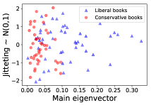
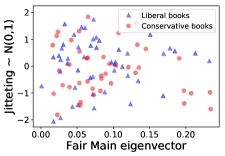
Figure 1: Projection of books (see Section 4) onto the first principal component. (Left) Original data. (Right) Data after spectral embedding. Books are ordered on the $x$ axis according to their corresponding entries in the main eigenvector, whereas on the $y$ axis we have random noise for visualization.

1.2 Related work

Densest Subgraph

Identifying dense subgraphs is a key primitive in a number of applications; see [13, 14, 15, 37]. The problem can be solved optimally in polynomial time [16]. On the contrary, the fair densest subgraph problem is highly related to the densest subgraph problem limited to at most $k$ nodes, which cannot be approximated up to a factor of $n^{1/(\log\log n)^{c}}$ for some $c>0$ assuming the exponential time hypothesis [23] and for which state-of-the-art methods yield an $O(n^{1/4+\varepsilon})$ approximation [5].

Algorithmic Fairness.

Fairness in algorithms received considerable attention in the recent past, see [17, 36, 38, 40] and references therein. The closely related notion of disparate impact was first proposed by [12]. It has since been used by [39] and Noriega-Campero et al. [28] for classification and Celis et al. [8, 9] for voting and ranking problems. Another problem that received considerable attention is fair clustering. This was first proposed as a problem by [11] in the case of a binary protected attribute. It was then investigated for various objectives and more color classes in theirs and subsequent work  [2, 3, 4, 19, 31, 33].

Most closely related to our work are the papers by [32, 35, 21]. The former two papers considers the problem of executing a principal component analysis in a fair manner. Specifically, given a matrix $A$ where the rows are colored (e.g. every row corresponds to a man or a woman), they ask for an algorithm that finds the finds a rank $k$ matrix $A^{\prime}$ whose residual error $\|A-A^{\prime}\|$ is small for both types of rows simultaneously. While our method is similarly based on using the principal component in a fair manner, the difference is that we may be forced to treat the classes differently, if we aim to uncover a dense subgraph as illustrated in the example mentioned above and in Figure 1.

The latter paper by [21] considers spectral clustering problems such as normalized cut. Like our work, they project the Laplacian matrix of a graph $G$ onto a suitable “fair” subspace, and then run $k$-means on the subspace spanned by the smallest resulting eigenvectors. Under a fair version of the stochastic block model, they show that this algorithm recovers planted fair partitions. Our work continues this idea by applying the technique to the densest subgraph problem.

1.3 Preliminaries and Notation

We consider undirected graphs $G(V,E,w)$, where $V$ is the set of $n$ nodes, $E\subset V\times V$ is the set of edges, and $w:E\rightarrow\mathbb{R}_{\geq 0}$ is a weight function. We denote the (weighted) adjacency matrix of $G$ by $A$. For a subset $E^{\prime}\subset E$ of the edges, we let $w(E^{\prime})=\sum_{e\in E^{\prime}}w(e)$. Considered $u\in V$, its (weighted) degree is ${d}_{u}=\sum_{e\cap\{v\}\neq\emptyset}w(e)$. We also let ${d}_{\max}=\max_{u}{d}_{u}$. Considered $S\subseteq V$, we denote by $G_{S}$ the induced subgraph. The density $D_{S}(G)$ of $S\subseteq V$ is simply the average degree of $G_{S}$, namely: namely:

$$D_{S}(G)=\frac{2\cdot\left|E\cap S\times S\right|}{\left|S\right|}.$$

We omit $G$ from $D_{S}(G)$, whenever clear from context.

A coloring of the vertices is simply a map $c:V\rightarrow[\ell]$ of $V$, where $[\ell]:=\{1,2,\dots,\ell$}. A set $S\subset V$ is called fair if $|S\cap\{v\in V~{}|~{}c(v)=1\}|=|S\cap\{v\in V~{}|~{}c(v)=2\}|=\dots=|S\cap\{v\in V~{}|~{}c(v)=\ell\}|$. A graph is called fair if $V$ is fair. In the remainder, we provide positive results for the important case $\ell=2$. In this case, for simplicity of exposition we denote the colors red and blue and we use $\textit{Red}:=\{v\in V~{}|~{}c(v)=\textit{red}\}$ and $\textit{Blue}:=\{v\in V~{}|~{}c(v)=\textit{blue}\}$ to refer to nodes of the respective color.

Definition 1 (Fair Densest Subgraph Problem).

Given a (weighted) graph $G(V,E,w)$ and a coloring $c$ of its vertices, identify a fair subset $S\subseteq V$ that maximizes $D_{S}$.

The fair densest subgraph problem is obviously a constrained version of the densest subgraph problem. It turns out to be considerably harder than its (polynomially solvable) unconstrained counterpart, as we show in Section 3.

Linear algebra notation.

We denote by $\lambda_{1}\geq\lambda_{2}\geq\ldots\geq\lambda_{n}$ the eigenvalues of $A$ and by $v_{i}$ its $i$-th eigenvector. We also set $\lambda=\max_{i>2}(\lambda_{2},|\lambda_{n}|)$. Note that we always have $\lambda_{1}\leq{d}_{\max}$. For a subset $S\subset V$, we denote by $\chi$ its normalized indicator vector, where $S$ is understood from context. Namely, $\chi_{i}=1/\sqrt{|S|}$ if $i\in S$, $\chi_{i}=0$ otherwise. Finally, for a vector $x\in\mathbb{R}^{n}$, we let $\|x\|=\sqrt{\sum_{i=1}^{n}x_{i}^{2}}$, the $2$-norm of $x$.

2 Spectral Relaxations for the Fair Densest Subgraph

As observed in Kannan and Vinay [20], the densest subgraph problem admits a spectral formulation. In particular, denoted by $x$ and indicator vector over the vertex set, the indicator vector of the vertex subset maxizing density is the maximizer of the following expression:

$$\max_{x\in\{0,1\}^{n}}\frac{x^{T}Ax}{x^{T}x}.$$

Now, assume that each node is colored with one of two colors, red or blue. The optimal solution $x^{*}$ might well overrepresent one of the colors. To formulate the problem of computing a fair solution, we can add the constraint

$$\sum_{\text{node~{}$i$ is red}}x_{i}=\sum_{\text{node~{}$i$ is blue}}x_{i}$$

$$\Leftrightarrow \sum_{\text{node~{}$i$ is red}}x_{i}\ -\sum_{\text{node~{}$i$ is blue}}x_{i}=0.$$

If we define the (unit $2$-norm) vector

$$f_{i}=\begin{cases}\frac{1}{\sqrt{n}}&\text{if node~{}$i$ is red}\\ -\frac{1}{\sqrt{n}}&\text{if node~{}$i$ is blue,}\end{cases}$$

the above constraint can be described as $f^{T}x=0$. We call such an $x$ fair. Conversely, very unbiased solutions will have high inner products with $f$.

Fair Densest Subgraph: Spectral Relaxation

Based on the considerations above, our approach transforms the input data (in this case the adjacency matrix $A$) by first projecting them onto the kernel of $f$. Namely, we first consider the following formulation of the fair densest subgraph problem:

$$\max_{x\in\{0,1\}^{n}}\frac{2x^{T}(I-ff^{T})A(I-ff^{T})x}{x^{T}x}.$$

It should be noted that, for any fair subset $S$ with indicator $x$, we have $\frac{2x^{T}Ax}{x^{T}x}=\frac{2x^{T}(I-ff^{T})A(I-ff^{T})x}{x^{T}x}.$ Conversely, for any indicator vector $x\notin span(I-ff^{T})$, the objective value can only decrease.

We next note that by relaxing $x$ to be an arbitrary vector, the above expression is maximized by the main eigenvector of $(I-ff^{T})A(I-ff^{T})$. Indeed, [20] established a relationship between the first eigenvector of the adjacency matrix $A$ and an approximately densest subgraph. Similar ideas are also implicit in the work of [25]. The above relaxation corresponds to replacing hard fairness constraints with soft ones. To prove our main result we need the following definition:

Definition 2.

Graph $H=(V_{H},E_{H})$ is $({d},\epsilon)$-regular if a ${d}$ exists, such that $(1-\epsilon){d}\leq{d}_{i}\leq(1+\epsilon){d}$, for every $i\in V_{H}$.

Theorem 1.

Assume we have a graph $G=(V,E,w)$ with a 2-coloring of the nodes. Assume the spectrum of $A$ satisfies $\lambda_{1}\geq 4\lambda$. Assume further that $G$ contains a fair subset $S$ such that: (1) $G_{S}$ is $({d},\epsilon)$-regular and (2) $d\geq(1-\theta){d}_{\max}$. In this case, it is possible to recover all but $16(\epsilon+\theta)|S|$ of the vertices in $S$ in polynomial time.

Intuitively, the result above states that, if the underlying network $G$ is an expander containing an almost-regular, dense and fair subgraph, we can approximately retrieve it in polynomial time. Succintly, this follows because, under these assumptions, the indicator vector of $S$ forms a small angle with the main eigenvector of $(I-ff^{T})A(I-ff^{T})$.

Proof of Theorem 1.

In the remainder of this proof, we denote by $\hat{\lambda}_{1}\geq,\ldots,\geq\hat{\lambda}_{n}$ the eigenvalues of $(I-ff^{T})A(I-ff^{T})$ and by $\hat{v}_{i}$ the $i$-th associated eigenvector. For a vertex $i$ of $G_{S}$ we denote by $\hat{{d}}_{i}$ its degree in $G_{S}$. We denote by $\chi$ the indicator vector of $S$ and we let $m=|S|$.

As a first step, we summarize straightforward, yet useful properties of the spectrum of $(I-ff^{T})A(I-ff^{T})$.

Lemma 1.

Whenever $\hat{\lambda}_{i}\neq 0$ we have:

$$(I-ff^{T})\hat{v}_{i}=\hat{v}_{i}\,\text{and }\,\hat{\lambda}_{i}=\hat{v}_{i}^{T}A\hat{v}_{i}$$ (1)

Proof.

If $\hat{\lambda}_{i}\neq 0$, we have:

$$(I-ff^{T})A(I-ff^{T})\hat{v}_{i}=\hat{\lambda}_{i}\hat{v}_{i}.$$

Since $(I-ff^{T})$ is a projection matrix, if we pre-multiply both members of the above equation by $(I-ff^{T})$ we have:

$$(I-ff^{T})A(I-ff^{T})\hat{v}_{i}=\hat{\lambda}_{i}(I-ff^{T})\hat{v}_{i}.$$

Subtracting the first equation from the second and recalling that $\hat{\lambda}_{i}\neq 0$ immediately the first claim.

The second claim follows immediately from the first:

$$\hat{\lambda}_{i}=\hat{v}_{i}^{T}(I-ff^{T})A(I-ff^{T})\hat{v}_{i}=\hat{v}_{i}^{T}A\hat{v}_{i}.$$

∎

It should be noted that, as a consequence of Lemma 1, we always have:

$$\hat{\lambda}_{1}=\hat{v}_{1}^{T}(I-ff^{T})A(I-ff^{T})\hat{v}_{1}=\hat{v}_{1}^{T}A\hat{v}_{1}\leq v_{1}^{T}Av_{1}=\lambda_{1}.$$

Note that this last property does not apply to the other eigenvalues in general. The first important, technical step to prove Theorem 1 is showing that the hypothesis $\lambda_{1}\geq 4\lambda$ implies that $\hat{\lambda}_{2}$ cannot be “too large”.

Lemma 2.

Assume the spectrum of $A$ satisfies the condition $\lambda_{1}\geq 4\lambda_{2}$. Then $\hat{\lambda}_{2}\leq\frac{3}{4}\lambda_{1}$.

Proof.

We first express $\hat{v}_{2}$ as $\hat{v}_{2}=\gamma v_{1}+z$, where $z$ is $\hat{v}_{2}$’s component orthogonal to $v_{1}$, the main eigenvector of $A$. Note that, since $v_{1}$ has unit norm, we have $\gamma^{2}+\|z\|^{2}=1$. Next:

$$\hat{\lambda}_{2}=(\gamma v_{1}+z)^{T}A(\gamma v_{1}+z)^{T}=\gamma\lambda_{1}+z^{T}Az,$$ (2)

where the first equality follows from Lemma 1, while the second follows since $z\in\mathbf{span}(v_{2},\ldots,v_{n})$ by definition and the $v_{i}$’s form an orthonormal basis. Next, assume $\gamma\geq 1/2$. In this case, we have:

$$\hat{\lambda}_{2}=\gamma\lambda_{1}+z^{T}Az=\gamma\lambda_{1}+\|z\|^{2}\frac{z^{T}Az}{\|z\|^{2}}\geq\frac{3}{8}\lambda_{1}.$$ (3)

Here, the third inequality follows since i) $\|z\|^{2}=1-\gamma^{2}\leq 1/2$, while $z\in\mathbf{span}(v_{2},\ldots,v_{n})$ implies:

$$\left|\frac{z^{T}Az}{\|z\|^{2}}\right|\leq\max_{w\perp v_{1}}\left|\frac{w^{T}Aw}{\|w\|^{2}}\right|=\lambda.$$

But (3) contradicts our assumption that $\lambda_{1}\geq 4\lambda$. On the other hand, if $\gamma\leq 1/2$, (2) implies:

$$\hat{\lambda}_{2}=\gamma\lambda_{1}+z^{T}Az\leq\gamma\lambda_{1}+z^{T}Az$$

$$\leq\gamma\lambda_{1}+\|z\|^{2}\max_{w\perp v_{1}}\frac{w^{T}Aw}{\|w\|^{2}}$$

$$=\gamma\lambda_{1}+(1-\gamma^{2})\lambda_{2}\leq\frac{\lambda_{1}}{2}+\lambda_{2}\leq\frac{3}{4}\lambda_{1}.$$

∎

The second step is showing that Lemma 2 implies that the indicator vector of the fair densest subgraph is close to $\hat{v}_{1}$:

Lemma 3.

Assume the the hypotheses of Theorem 1 hold. Then:

$$\|\chi-\hat{v}_{1}\|^{2}\leq 4(\epsilon+\theta).$$

Proof.

We begin by noting that $\chi^{T}f=0$ by definition, which implies $(I-ff^{T})\chi=\chi$. We therefore have:

$$\chi^{T}(I-ff^{T})A(I-ff^{T})\chi=\frac{\sum_{i\in S}\hat{d}_{i}}{m}\geq(1-\epsilon)d,$$ (4)

Next, we decompose $\chi$ along its components respectively parallel and orthogonal to $\hat{v}_{1}$, namely, $\chi=\alpha\hat{v}_{1}+z$, and we note that $\|z\|^{2}=1-\alpha^{2}$, since both $\hat{v}_{1}$ and $\chi$ are unit norm vectors. Set $B=(I-ff^{T})A(I-ff^{T})$ for the sake of space. We have:

$$\chi^{T}B\chi=(\alpha\hat{v}_{1}+z)^{T}Bs(\alpha\hat{v}_{1}+z)=\alpha^{2}\hat{\lambda}_{1}+z^{T}Bz$$

$$\leq\alpha^{2}\hat{\lambda}_{1}+\hat{\lambda}_{2}\|z\|^{2}\leq\alpha^{2}\hat{\lambda}_{1}+(1-\alpha^{2})\hat{\lambda}_{2}.$$ (5)

Putting together (4) and (5) yields $\alpha^{2}\geq\frac{(1-\epsilon){d}-\hat{\lambda}_{2}}{\hat{\lambda}_{1}-\hat{\lambda}_{2}}$. Now:

$$\|\chi-v\|^{2}\leq 1-\frac{(1-\epsilon){d}-\hat{\lambda}_{2}}{\hat{\lambda}_{1}-\hat{\lambda}_{2}}$$

$$\leq 1-\frac{(1-\epsilon)(1-\theta){d}_{\max}-\hat{\lambda}_{2}}{\lambda_{1}-\hat{\lambda}_{2}}$$

$$\leq 1-\frac{(1-\epsilon)(1-\theta)\lambda_{1}-\hat{\lambda}_{2}}{\lambda_{1}-\hat{\lambda}_{2}}$$

$$<1-\frac{\lambda_{1}-\hat{\lambda}_{2}-(\epsilon+\theta)\lambda_{1}}{\lambda_{1}-\hat{\lambda}_{2}}$$

$$=\frac{(\epsilon+\theta)\lambda_{1}}{\lambda_{1}-\hat{\lambda}_{2}}\leq 4(\epsilon+\theta).$$

Here, the second inequality follows from our hypotheses on ${d}$ and since $\hat{\lambda}_{1}\leq\hat{\lambda}$, the third inequality follows since the main eigenvalue of an adjacency matrix is upper-bounded by the maximum degree of the underlying graph, while the last inequality follows from Lemma 2. ∎

Corollary 1.

Under the hypotheses of Lemma 3, for all but at most $16m(\epsilon+\theta)$ vertices in $V$ we have: i) $\hat{v}_{1}(i)\geq\frac{1}{2\sqrt{m}}$ if $i\in S$, ii) $\hat{v}_{1}(i)<\frac{1}{2\sqrt{m}}$ otherwise.

Proof.

We first note that the number of vertices $i$ for which $\left|\hat{v}_{1}(i)-\chi(i)\right|>\frac{1}{2\sqrt{m}}$ is at most $16m(\epsilon+\theta)$. To see why, assume there are $x$ such vertices. This implies $\|\hat{v}_{1}-\chi\|^{2}\geq\frac{x}{4m}.$ On the other hand, the upper bound following from Lemma 3 immediately implies $x\leq 16m(\epsilon+\theta)$. Next, recall that $\chi_{i}=\frac{1}{\sqrt{m}}$ if $i\in S$, $\chi_{i}=0$ otherwise. This immediately implies the thesis. ∎

The algorithm

Our algorithm is based on a sweep of $\hat{v}_{1}$ [20, 25]. In particular, we run Algorithm GSA (see Algorithm 1) with $M=(I-ff^{T})A(I-ff^{T})$ and $\Delta=16(\epsilon+\theta)$.

1 Algorithm:  General Sweep Algorithm (GSA)

Data: Non-negative $n\times n$ matrix $M$, parameter $\Delta$

Result: Subset $S\subseteq V$

2 $\hat{S}=\emptyset$; $\hat{D}=0$;

3

4Compute $v_{1}=$ main eigenvector of $M$;

5

6Sort nodes $i\in V$ in non increasing order of $v_{1}(i)$;

7

8// Assume w.l.o.g. that $\{1,\ldots,n\}$ is resulting ordering of nodes in $V$ ;

9

10for $s=1$ to $n$ do

11       $S=\{1,\ldots,s\}$

12       Compute $D_{S}=$ density of the subgraph induced by $S$

13       if $D_{S}>\hat{D}$ AND $\left||S\cap Red|-|S\cap Blue|\right|\leq\Delta|S|$ then

14             $\hat{S}=S$; $\hat{D}=D_{S}$

15            

16       end if

17      

18 end for

return $\hat{S}$

Algorithm 1 General Sweep Algorithm (non-increasing).

Corollary 1 ensures that i) the above algorithm always returns a solution, ii) the solution returned by the algorithm will not be worse than the one obtained by picking $i$ if $\hat{v}_{1}(i)\geq\frac{1}{2\sqrt{m}}$ and rejecting it otherwise. This concludes the proof of Theorem 1. ∎

3 Hard Constraints and Hardness of Approximation

In general, enforcing fairness can make an “easy” problem intractable and this is the case for the densest subgraph problem. In this context, spectral relaxations can be regarded as a way to mitigate this issue, by enforcing soft fairness constraints to virtually any problem that is amenable to an algebraic formulation.

Nevertheless, in some cases it might be important to assess the price of fairness, by comparing the achievable quality of fair solutions to that of solutions for the original, unconstrained problem. In this section, we complement our algorithmic treatment of fairness with hardness results and approximation algorithms for specific cases. Some of our hardness results are based on the small set expansion hypothesis, which we now describe.

Consider a $d$-regular weighted graph $G$ and, for every $S\subset V$, denote by $\Phi(S)$ the expansion of $S$ [30]. Given two constants $\delta,\eta\in(0,1)$, the small set expansion problem [30] $SSE(\delta,\eta)$ asks to distinguish between the following two cases:

Completeness

There exists a set of nodes $S\subset V$ of size $\delta\cdot|V|$ such that $\Phi(S)\leq\eta$.

Soundness

For every set of nodes $S\subset V$ of size $\delta\cdot|V|$, $\Phi(S)\geq 1-\eta$.

Our hardness proofs are based on the small set expansion hypothesis defined as follows.

Conjecture 1 (SSEH).

For every $\eta>0$ there exists a $\delta:=\delta(\eta)>0$ such that $SSE(\eta,\delta)$ is NP-hard.

3.1 General Case

Given a weighted graph $G(V,E,w)$, the densest subgraph problem asks to find a set of nodes $S$ such that the density $D_{S}:=\frac{|E_{S}|}{|S|}$ is maximized. The fair densest subgraph problem additionally requires $S$ to be fair.

The densest at-most-$k$ subgraph problem asks to find a set of nodes $S$ with $|S|\leq k$, such that the density $D_{S}:=\frac{|E_{S}|}{|S|}$ is maximized. Recall from Section 1.2 that, whereas the densest subgraph problem is polynomially solvable, the best approximation for the densest at-most-$k$ subgraph problem is in $O(n^{1/4})$ [6] and cannot be approximated up to a factor of $n^{1/(\log\log n)^{c}}$ for some $c>0$ assuming the exponential time hypothesis [23] . The next theorem implies that these inapproximability results for the densest at-most-$k$ subgraph problem hold also for the fair densest subgraph problem, showing that fairness constraints can drastically affect hardness of this problem.

Theorem 2.

Computing an $\alpha$-approximation for the fair densest subgraph problem is at least as hard as computing an $\alpha$-approximation for the densest at-most-$k$ subgraph problem. Moreover, any $\alpha$-approximation to the densest at-most-$k$ subgraph is an $2\alpha$ approximation to densest fair subgraph.

Proof.

Consider an arbitrary graph $G(V,E)$. We consider $V$ to be colored red. Add $k$ blue nodes with no edges. Then the density of the fair densest subgraph is, up to a multiplicative factor of exactly $\frac{1}{2}$, equal to the density of the densest at most $2k$ subgraph.

The argument for the upper bound is completely analogous to the proof given for Theorem 3. ∎

When the input graph $G$ is itself fair, we can provide stronger bounds.

1 Input: Graph $G(V,E,w)$

2 1: Compute the densest subgraph $S$

3 2: W.l.o.g $|S\cap Blue|\geq|S\cap Red|$

4 3: While $|S\cap Blue|>|S\cap Red|$, add an arbitrary node $v\in Red\setminus S$ to $S$

4: Return $S$

Algorithm 2 Approximate Fair Densest Subgraph

Theorem 3.

Given a fair graph $G(V,E,w)$, Algorithm 2 computes a fair set $S\subset V$, such that $D_{S}\cdot 2\geq OPT$, where $OPT$ is the density of the fair densest subgraph. Similarly, any $\alpha$-approximation to densest at-most-$k$ subgraph is an $2\alpha$ approximation to densest fair subgraph.

Proof.

We refer to the set $S$ computed after line $1$, and $3$ as $S_{1}$ an $S_{2}$, respectively. Since $S_{1}$ is the unconstrained densest subgraph, $D_{S_{1}}>OPT$. For $S_{2}$, we observe that $|S_{2}|\leq S_{1}+|S_{1}\cap Blue|-|S_{1}\cap Red|\leq 2\cdot|S_{1}|$, hence

$$D_{S_{2}}=\frac{w(E_{S_{2}})}{|S_{2}|}\geq\frac{w(E_{S_{1}})}{2|S_{1}|}\geq\frac{OPT}{2}.$$

To conclude the proof, we observe that $S_{2}$ is always fair. ∎

We conclude this section by showing that approximating the fair densest subgraph problem beyond a factor of $2$ is at least as hard as solving $SSE(\eta,\delta)$. Therefore, barring a major algorithmic breakthrough, Algorithm 2 is optimal. The proof is provided as supplementary material and it is based on the following idea: In regular graphs, for a given set of nodes $S$, the expansion $\Phi(S)$ is related to the density of $S$. We can use this, so that, given a graph $G$, we can carefully construct a colored graph $G^{\prime}$ such that finding the optimal fair densest subgraph in $G^{\prime}$ gives an estimate of the largest-expansion node set in $G$.

Theorem 4.

If SSEH holds, computing a $(2-\varepsilon)$ approximation of the fair densest subgraph problem in fair graphs is $NP$-hard for any $\varepsilon>0$.

Proof.

We consider the $SSE(\eta,\delta)$ problem, i.e. let $G(V,E,w)$ be a $d$-regular graph and let $\eta\in(0,1)$ and $\delta=\delta(\eta)\in(0,1/2]$ be constants that we will specify later. For any set $S\subset V$ of size $s:=\delta\cdot|V|$, we have $w(E_{S}):=d\cdot s-\Phi(S)\cdot d\cdot s$.

We construct a colored graph $G^{\prime}(V^{\prime},E^{\prime},w^{\prime})$ by considering all nodes of $G$ to be colored red, and by adding $|V|$ blue nodes. Of these nodes, we select an arbitrary but fixed subset of $\delta\cdot|V|$ blue nodes that we denote by $B$. Each edge in $E_{B}$ is weighted uniformly by $t:=\frac{2\cdot d}{s-1}$. The remaining edges are weighted with $0$.

Recall that SSEH states that distinguishing between the two cases is $NP$-hard.

Completeness

If there exists some $S\subset V$ of size $s$ with $\Phi(S)\leq\eta$, then

$$w(E_{S})\geq(1-\eta)\cdot d\cdot s.$$

Then the density of the fair subgraph induced by $S\cup B$ of size $2s$ satisfies

$$D_{S\cup B} = \frac{w(E_{S})+w(B)}{2|S|}\geq\frac{(1-\eta)\cdot d\cdot s+t\cdot{s\choose 2}}{2s}$$ (6)

$$= \frac{(1-\eta)\cdot d+t\cdot\frac{s-1}{2}}{2}\geq(1-\eta)\cdot d.$$

Soundness

If for all $S\subset V$ of size $s$, $\Phi(S)\geq 1-\eta$, then

$$w(E_{S})\leq\eta\cdot d\cdot s.$$ (7)

Denote the size of the fair densest subgraph $C$ by $k$. Further, let $C_{red}=C\cap Red$. We will distinguish between four basic cases: (1) $k<2\mu\cdot s$, (2) $2\mu\cdot s\leq k<2\cdot s$, (3) $2\cdot s\leq k<\frac{2}{\mu}s$, and (4) $\frac{2}{\mu}s\leq k$, where $\mu>0$ is suitably small constant specified later. We note that the cases (1) and (4) and (2) and (3) will turn out to be somewhat symmetric, even if slightly different proofs are required in every case.

First, let $k<2\mu\cdot s$ and again let $B_{k}$ be an arbitrary subset of $B$ of size $k$. Then

$$D_{C_{red}\cup B_{k}} \leq \frac{d\cdot k+w(B_{k})}{2\cdot k}=\frac{d\cdot k+t\cdot{k\choose 2}}{2\cdot k}$$ (8)

$$= \frac{d+t\cdot\frac{k-1}{2}}{2}=\frac{d}{2}+\frac{d\cdot(k-1)}{2(s-1)}$$

$$\leq \frac{d}{2}+\frac{d\cdot 2\mu}{2}\leq(1+2\mu)\frac{d}{2},$$

where the first inequality holds due to regularity.

Now, let $2\mu\cdot s\leq k<2\cdot s$. We have

$$D_{C_{red}\cup B_{k}} \leq \frac{\eta\cdot d\cdot s+w(B_{k})}{2\cdot k}$$ (9)

$$= \frac{\eta\cdot d\cdot s}{2\cdot k}+\frac{d\cdot(k-1)}{2\cdot(s-1)}$$

$$\leq \frac{\eta\cdot d}{\mu}+\frac{d}{2}\leq\left(1+\frac{2\eta}{\mu}\right)\frac{d}{2}.$$

Now, let $2\cdot s\leq k\leq\frac{2}{\mu}\cdot s$. We will first show that

$$w(C)\leq\frac{2}{\mu}\cdot\eta\cdot d\cdot k.$$ (10)

For the sake of contradiction, assume that this is not the case. The argument revolves around double counting $w(C)$. There exist ${k\choose s}$ subsets of size $s$ of $C$. Observe that for any such subset $S^{\prime}$ has weight $w(S^{\prime})\leq\eta\cdot d\cdot s$ and hence

$$\sum_{S^{\prime}\subset C~{}\wedge~{}|S^{\prime}|=s}w(S^{\prime})\leq\eta\cdot d\cdot s\cdot{k\choose s}.$$

At the same time, every (possibly $0$ valued) edge appears in ${k-2\choose s-2}$ of these subsets. Hence

$$\sum_{S^{\prime}\subset C~{}\wedge~{}|S^{\prime}|=s}w(S^{\prime})=w(C)\cdot{k-2\choose s-2}>\frac{2}{\mu}\cdot\eta\cdot d\cdot k\cdot{k-2\choose s-2}.$$

Combining both equations, we have

$$\frac{2}{\mu}\cdot\eta\cdot d\cdot k\cdot{k-2\choose s-2}<\eta\cdot d\cdot s\cdot{k\choose s}$$

$$\Leftrightarrow\frac{2}{\mu}<\frac{k\cdot(k-1)}{s\cdot(s-1)}\frac{s}{k}\leq\frac{2}{\mu},$$

which is a contradiction.

Consider now the density of any fair cut containing $C\cup B_{k}$, where $B_{k}$ contains $B$ and $k-s$ further arbitrary blue nodes. We have

$$D_{C_{red}\cup B_{k}} \leq \frac{\frac{2\eta}{\mu}\cdot d\cdot k+t\cdot{s\choose 2}}{2\cdot k}$$ (11)

$$= \frac{\eta}{\mu}\cdot\frac{d}{2}+\frac{d\cdot s}{2\cdot k}\leq\left(1+\frac{2\eta}{\mu}\right)\cdot\frac{d}{2}.$$

Finally, consider the case $k>\frac{2}{\mu}s$. Then the density of any fair cut containing $C\cup B_{k}$, where $B_{k}$ contains $B$ and $k-s$ further arbitrary blue nodes, is

$$D_{C_{red}\cup B_{k}} \leq \frac{d\cdot k+t\cdot{s\choose 2}}{2\cdot k}$$ (12)

$$= \frac{d}{2}+\frac{d\cdot s}{2\cdot k}\leq\leq(1+2\mu)\frac{d}{2}.$$

We note that bounds from Equations 8 and 11 and Equations 9 and 12 are identical. For $\varepsilon<\frac{1}{4}$, we set $\mu=\frac{\varepsilon}{2}$, $\eta\leq\frac{8}{3}\cdot\varepsilon^{2}$. Then the ratio between the terms 6 and 8 and the terms 6 and 9 is at least $2-\varepsilon$. Therefore, approximating the fair densest subgraph problem beyond a factor of $2$ solves the $SSE(\eta,\delta)$ problem. ∎

4 Experimental Analysis

Worst case bounds are often uninformative when compared with empirical behavior. Algorithm 2 is (assuming that the underlying graph is fair) theoretically optimal and therefore superior to the spectral recovery schemes. As we now describe, the empirical performance between these approaches paints the opposite picture.

Overview.

To test the performances of our algorithms on real data we used two publicly available dataset: PolBooks [1] and Amazon products metadata [27]. Both (explicitly or implicitly) contain undirected unweighted graphs, whose nodes are products from the Amazon catalog, while an edge between two nodes exists if the corresponding products are frequently co-purchased by the same buyer. Moreover, for both datasets, each product belongs to exactly one category.

We tested our methods in a scenario in which, given a (not necessary fair) labelled graph, our only interest lies in finding fair subgraphs with high density. In this context, we are considering the density of the provided solution as a quality indicator: more dense reflects more quality.

For our experiments we used an Intel Xeon 2.4GHz with 24GB of RAM running Linux Ubuntu 18.04 LTS.

Datasets.

The PolBooks data set [1] is an undirected unweighted graph, whose nodes represent books on US politics included in the Amazon catalog, while an edge between two books exists if both books are frequently co-purchased by the same buyer. Each book is further labeled depending on its political stance, possible labels being “liberal”, “neutral”, and “conservative”. For our experiments, we considered only the subgraph induced by “liberal” and “conservative” books, obtaining 92 nodes (49 of which were associated with a “conservative” worldview, 43 with a “liberal” worldview) for 362 edges in total.

The Amazon products metadata dataset [27] contains descriptions for 15.5 million Amazon products . For a single product, we only considered the product id (asin field), the category the product belongs to (main_cat field) and the set of frequently co-purchased products (also_buy field). It should be noted that in this dataset, each node belongs to exactly one (main) Amazon category so that, together, these three fields allow recovery of a large, undirected, labelled graph, with products as nodes, categories as labels and edges representing frequent co-purchasing product pairs. For this data set, we leveraged the co-purchasing relation among products, to naturally extract undirected and unweighted, labelled graphs. In more detail, for each pair $(\ell_{1},\ell_{2})$ of Amazon main categories, we extracted the undirected subgraph induced by the subset of nodes of category $\ell_{1}$ ($\ell_{2}$) that have at least one neighbour from category $\ell_{2}$ ($\ell_{1}$). We did not consider graphs with fewer than 100 nodes. This way, we retrieved 292 subgraphs, with sizes ranging between 100 and 22046 nodes.

Algorithms.

We compared the performance of the following algorithms:

2-DFSG. The optimal 2-approximation algorithm (Algorithm 2) based on Goldberg’s optimal algorithm for the densest subgraph problem [16], described in Section 3.

Spectral Algorithms. Following [20, 25] and Theorem 1, we ran a variety of eigenvector rounding algorithms. These are all variants of a modified version of the General Sweep Algorithm (Algorithm 1) used in the proof of Theorem 1 that sorts the entries of the main eigenvector of $M$ four times (instead of a single one) according to the following criteria: i) non-increasing; ii) non-decreasing; iii) non-increasing absolute values; iv.) non decreasing absolute values. With these premises, we consider the following spectral algorithms. The first two are just the modified version of Algorithm 1 with different choices for $M$, while PS and FPS perform a slightly modified sweep that always affords a fair solution.

Single Sweep (SS). This algorithm is simply (Algorithm 1), when all previously mentioned sorting criteria are used, with $M=A$ and $\Delta=0$.

Fair Single Sweep (FSS). It is the execution of SS, this time on matrix $(I-ff^{T})A(I-ff^{T})$ instead of $A$.

Paired Sweep (PS). Paired Sweep is a modification of SS in which the fairness constraint is satisfied by construction in each subgraph produced by the rounding algorithm. This is done by considering the subsets $V_{\textit{Red}}$ and $V_{\textit{Blue}}$ of the nodes, sorting each of them separately according to the values of the corresponding entries in the main eigenvector of $A$ and then, for each $s=1,\ldots,\min({|V_{\textit{Red}}|,|V_{\textit{Blue}}|})$ considering the candidate set of nodes of cardinality $2s$ obtained by taking the first $s$ nodes from each ordered subset.

Fair Paired Sweep (FPS). It is the execution of PS, this time on matrix $(I-ff^{T})A(I-ff^{T})$ instead of $A$.

4.1 Results

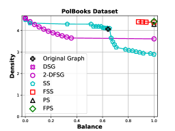
Figure 2: Pareto front of the subgraphs generated by each algorithm, w.r.t. density and balance, on PolBooks dataset.

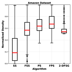
Figure 3: Performance of our algorithms on Amazon dataset on 292 samples. Reported are aggregates over all generated subgraphs, with unfair solutions receiving a density of $0$, see Table 1.

Figure 2 shows the performance of our algorithms on PolBooks dataset through the Pareto front of the subgraphs generated by each algorithm during its execution w.r.t. density and balance . PS and FPS by construction only return fair solutions while the other algorithms potentially have trade-offs. In particular, 2-DSG (Algorithm 2) starts at the unconstrained optimum and proceeds to add nodes that increase balance while potentially decreasing density.

Figure 3 shows the distributions of the normalized density, over the entire set of Amazon instances, of the fair subgraphs retrieved by different algorithms. Normalization, performed to make solutions for different instances comparable, is done by scaling to the optimal density of the unconstrained problem. With the exception of SS, which uses the original adjacency matrix and whose distribution is skewed toward lower density values, performances of spectral heuristics are comparable, with FPS achieving highest median density. In general spectral algorithms run on $(I-ff^{T})A(I-ff^{T})$ (FSS and FPS) respectively outperform their counterparts (SS and PS) run on $A$. Interestingly, with the exception of SS, spectral heuristics consistently outperform 2-DFSG, despite its theoretical optimality.

We report in Table 1 the percentage of instances each algorithm is not able to solve, i.e., for which it does not return a fair solution and, consequently, we assigned a density equal to $0$.

SS	FSS	PS	FPS	2-DFSG
1.03	0.34	0	0	3.08

Table 1: Percentages of unfair solutions over 292 samples for Amazon dataset. As noted previously, PS and FPS cannot return unfair solutions. $2$-DFSG (Algorithm 2) results in an unfair solutions if the original graph is unbalanced and the unconstrained densest subgraph cannot be made fair via line 3.

5 Conclusion and Future Work

In this work, we studied graphs with an arbitrary $2$-coloring. For these graphs, the densest fair subgraph problem consists of finding a subgraph with maximal induced degree under the condition that both colors occur equally often. We observed that the problem is closely related to the densest at most k subgraph problem and thus has similar strong inapproximability results. On the positive side, we presented an optimal approximation algorithm under the assumption that the graph itself is fair, and a more involved spectral recovery algorithm inspired by the work of [21] on stochastic block models.

In practice, the spectral recovery algorithm tended to dominate the approximation algorithm. We interpret these results as showing that (1) an approximation algorithm may not be the correct way to attack this problem, and (2) as previous work also suggests [32, 21], spectral relaxations seem to be an inexpensive tool to improve the fairness of algorithms geared towards recovery and learning.

Future work might consider extending this approach to more involved fairness constraints. As noted by [21], the ideal of removing “unfairness” via orthogonal projections straightforwardly generalized to multiple and potentially overlapping color classes. However, analyzing the spectrum in these cases seems to be significantly more difficult.

References

- [1] Polbook-network-dataset, v. krebs, unpublished. http://www.orgnet.com/.
- [2] Arturs Backurs, Piotr Indyk, Krzysztof Onak, Baruch Schieber, Ali Vakilian, and Tal Wagner. Scalable fair clustering. In Proceedings of the 36th International Conference on Machine Learning, ICML 2019, 9-15 June 2019, Long Beach, California, USA, pages 405–413, 2019.
- [3] Suman Kalyan Bera, Deeparnab Chakrabarty, Nicolas Flores, and Maryam Negahbani. Fair algorithms for clustering. In Advances in Neural Information Processing Systems 32: Annual Conference on Neural Information Processing Systems 2019, NeurIPS 2019, 8-14 December 2019, Vancouver, BC, Canada, pages 4955–4966, 2019.
- [4] Ioana O. Bercea, Martin Groß, Samir Khuller, Aounon Kumar, Clemens Rösner, Daniel R. Schmidt, and Melanie Schmidt. On the cost of essentially fair clusterings. CoRR, abs/1811.10319, 2018.
- [5] Aditya Bhaskara, Moses Charikar, Eden Chlamtac, Uriel Feige, and Aravindan Vijayaraghavan. Detecting high log-densities: an O(n) approximation for densest k-subgraph. In Proceedings of the 42nd ACM Symposium on Theory of Computing, STOC 2010, Cambridge, Massachusetts, USA, 5-8 June 2010, pages 201–210, 2010.
- [6] Aditya Bhaskara, Moses Charikar, Aravindan Vijayaraghavan, Venkatesan Guruswami, and Yuan Zhou. Polynomial integrality gaps for strong SDP relaxations of densest k-subgraph. In Proceedings of the Twenty-Third Annual ACM-SIAM Symposium on Discrete Algorithms, SODA 2012, Kyoto, Japan, January 17-19, 2012, pages 388–405, 2012.
- [7] Levi Boxell, Matthew Gentzkow, and Jesse Shapiro. Is the internet causing political polarization? evidence from demographics. Technical report, mar 2017.
- [8] L. Elisa Celis, Lingxiao Huang, and Nisheeth K. Vishnoi. Multiwinner voting with fairness constraints. In Proceedings of the Twenty-Seventh International Joint Conference on Artificial Intelligence, IJCAI 2018, July 13-19, 2018, Stockholm, Sweden., pages 144–151, 2018.
- [9] L. Elisa Celis, Damian Straszak, and Nisheeth K. Vishnoi. Ranking with fairness constraints. In 45th International Colloquium on Automata, Languages, and Programming, ICALP 2018, July 9-13, 2018, Prague, Czech Republic, pages 28:1–28:15, 2018.
- [10] Tanmoy Chakraborty, Ayushi Dalmia, Animesh Mukherjee, and Niloy Ganguly. Metrics for community analysis: A survey. ACM Comput. Surv., 50(4):54:1–54:37, 2017.
- [11] Flavio Chierichetti, Ravi Kumar, Silvio Lattanzi, and Sergei Vassilvitskii. Fair clustering through fairlets. In Proceedings of the 30th Annual Conference on Neural Information Processing Systems (NIPS), pages 5036–5044, 2017.
- [12] Michael Feldman, Sorelle A. Friedler, John Moeller, Carlos Scheidegger, and Suresh Venkatasubramanian. Certifying and removing disparate impact. In Proceedings of the 21th ACM SIGKDD International Conference on Knowledge Discovery and Data Mining, pages 259–268, 2015.
- [13] Eugene Fratkin, Brian T Naughton, Douglas L Brutlag, and Serafim Batzoglou. Motifcut: regulatory motifs finding with maximum density subgraphs. Bioinformatics, 22(14):e150–e157, 2006.
- [14] David Gibson, Ravi Kumar, and Andrew Tomkins. Discovering large dense subgraphs in massive graphs. In Proceedings of the 31st International Conference on Very Large Data Bases, Trondheim, Norway, August 30 - September 2, 2005, pages 721–732, 2005.
- [15] Aristides Gionis, Flavio Junqueira, Vincent Leroy, Marco Serafini, and Ingmar Weber. Piggybacking on social networks. Proceedings of the VLDB Endowment, 6(6):409–420, 2013.
- [16] A. V. Goldberg. Finding a maximum density subgraph. Technical Report UCB/CSD-84-171, EECS Department, University of California, Berkeley, 1984.
- [17] Moritz Hardt, Eric Price, and Nati Srebro. Equality of opportunity in supervised learning. In Advances in Neural Information Processing Systems 29: Annual Conference on Neural Information Processing Systems 2016, December 5-10, 2016, Barcelona, Spain, pages 3315–3323, 2016.
- [18] Sujin Horwitz. The compositional impact of team diversity on performance: Theoretical considerations. Human Resource Development Review, 4:219–245, 06 2005.
- [19] Lingxiao Huang, Shaofeng H.-C. Jiang, and Nisheeth K. Vishnoi. Coresets for clustering with fairness constraints. In Hanna M. Wallach, Hugo Larochelle, Alina Beygelzimer, Florence d’Alché-Buc, Emily B. Fox, and Roman Garnett, editors, Advances in Neural Information Processing Systems 32: Annual Conference on Neural Information Processing Systems 2019, NeurIPS 2019, 8-14 December 2019, Vancouver, BC, Canada, pages 7587–7598, 2019.
- [20] Ravi Kannan and V Vinay. Analyzing the structure of large graphs. 1999.
- [21] Matthäus Kleindessner, Samira Samadi, Pranjal Awasthi, and Jamie Morgenstern. Guarantees for spectral clustering with fairness constraints. In Proceedings of the 36th International Conference on Machine Learning, ICML 2019, 9-15 June 2019, Long Beach, California, USA, pages 3458–3467, 2019.
- [22] Theodoros Lappas, Kun Liu, and Evimaria Terzi. Finding a team of experts in social networks. In Proceedings of the 15th ACM SIGKDD International Conference on Knowledge Discovery and Data Mining, KDD ’09, pages 467–476, 2009.
- [23] Pasin Manurangsi. Almost-polynomial ratio eth-hardness of approximating densest k-subgraph. In Proceedings of the 49th Annual ACM SIGACT Symposium on Theory of Computing, STOC 2017, Montreal, QC, Canada, June 19-23, 2017, pages 954–961, 2017.
- [24] Leandro Soriano Marcolino, Albert Xin Jiang, and Milind Tambe. Multi-agent team formation: diversity beats strength? In Twenty-Third International Joint Conference on Artificial Intelligence, 2013.
- [25] Frank McSherry. Spectral partitioning of random graphs. In 42nd Annual Symposium on Foundations of Computer Science, FOCS 2001, 14-17 October 2001, Las Vegas, Nevada, USA, pages 529–537, 2001.
- [26] Cameron Musco, Christopher Musco, and Charalampos E. Tsourakakis. Minimizing polarization and disagreement in social networks. In Proceedings of the 2018 World Wide Web Conference on World Wide Web, WWW 2018, Lyon, France, April 23-27, 2018, pages 369–378, 2018.
- [27] Jianmo Ni, Jiacheng Li, and Julian McAuley. Justifying recommendations using distantly-labeled reviews and fine-grained aspects. In Proceedings of the 2019 Conference on Empirical Methods in Natural Language Processing and the 9th International Joint Conference on Natural Language Processing (EMNLP-IJCNLP), pages 188–197, Hong Kong, China, November 2019. Association for Computational Linguistics.
- [28] Alejandro Noriega-Campero, Michiel Bakker, Bernardo Garcia-Bulle, and Alex Pentland. Active fairness in algorithmic decision making. CoRR, abs/1810.00031, 2018.
- [29] Prasad Raghavendra and David Steurer. Graph expansion and the unique games conjecture. In Proceedings of the 42nd ACM Symposium on Theory of Computing, STOC 2010, Cambridge, Massachusetts, USA, 5-8 June 2010, pages 755–764, 2010.
- [30] Prasad Raghavendra and David Steurer. Graph expansion and the unique games conjecture. In Proceedings of the 42nd ACM Symposium on Theory of Computing, STOC 2010, Cambridge, Massachusetts, USA, 5-8 June 2010, pages 755–764, 2010.
- [31] Clemens Rösner and Melanie Schmidt. Privacy preserving clustering with constraints. In 45th International Colloquium on Automata, Languages, and Programming, ICALP 2018, July 9-13, 2018, Prague, Czech Republic, pages 96:1–96:14, 2018.
- [32] Samira Samadi, Uthaipon Tao Tantipongpipat, Jamie H. Morgenstern, Mohit Singh, and Santosh Vempala. The price of fair PCA: one extra dimension. In Advances in Neural Information Processing Systems 31: Annual Conference on Neural Information Processing Systems 2018, NeurIPS 2018, 3-8 December 2018, Montréal, Canada., pages 10999–11010, 2018.
- [33] Melanie Schmidt, Chris Schwiegelshohn, and Christian Sohler. Fair coresets and streaming algorithms for fair k-means. In Approximation and Online Algorithms - 17th International Workshop, WAOA 2019, Munich, Germany, September 12-13, 2019, Revised Selected Papers, pages 232–251, 2019.
- [34] Mauro Sozio and Aristides Gionis. The community-search problem and how to plan a successful cocktail party. In Proceedings of the 16th ACM SIGKDD International Conference on Knowledge Discovery and Data Mining, Washington, DC, USA, July 25-28, 2010, pages 939–948, 2010.
- [35] Uthaipon Tantipongpipat, Samira Samadi, Mohit Singh, Jamie H. Morgenstern, and Santosh S. Vempala. Multi-criteria dimensionality reduction with applications to fairness. In Hanna M. Wallach, Hugo Larochelle, Alina Beygelzimer, Florence d’Alché-Buc, Emily B. Fox, and Roman Garnett, editors, Advances in Neural Information Processing Systems 32: Annual Conference on Neural Information Processing Systems 2019, NeurIPS 2019, 8-14 December 2019, Vancouver, BC, Canada, pages 15135–15145, 2019.
- [36] Binh Luong Thanh, Salvatore Ruggieri, and Franco Turini. k-nn as an implementation of situation testing for discrimination discovery and prevention. In Proceedings of the 17th ACM SIGKDD International Conference on Knowledge Discovery and Data Mining, pages 502–510, 2011.
- [37] Charalampos E. Tsourakakis, Francesco Bonchi, Aristides Gionis, Francesco Gullo, and Maria A. Tsiarli. Denser than the densest subgraph: extracting optimal quasi-cliques with quality guarantees. In The 19th ACM SIGKDD International Conference on Knowledge Discovery and Data Mining, KDD 2013, Chicago, IL, USA, August 11-14, 2013, pages 104–112, 2013.
- [38] Muhammad Bilal Zafar, Isabel Valera, Manuel Gomez Rodriguez, and Krishna P. Gummadi. Fairness beyond disparate treatment & disparate impact: Learning classification without disparate mistreatment. In Proceedings of the 26th International Conference on World Wide Web (WWW), pages 1171–1180, 2017.
- [39] Muhammad Bilal Zafar, Isabel Valera, Manuel Gomez-Rodriguez, and Krishna P. Gummadi. Fairness constraints: Mechanisms for fair classification. In Proceedings of the 20th International Conference on Artificial Intelligence and Statistics, AISTATS 2017, 20-22 April 2017, Fort Lauderdale, FL, USA, pages 962–970, 2017.
- [40] Muhammad Bilal Zafar, Isabel Valera, Manuel Gomez-Rodriguez, Krishna P. Gummadi, and Adrian Weller. From parity to preference-based notions of fairness in classification. In Advances in Neural Information Processing Systems 30: Annual Conference on Neural Information Processing Systems 2017, 4-9 December 2017, Long Beach, CA, USA, pages 228–238, 2017.