Stochastic fluctuations of bosonic dark matter

Numerous theories extending beyond the standard model of particle physics predict the existence of bosons Dimopoulos and Giudice (1996); Arkani-Hamed et al. (2000); Taylor and Veneziano (1988); Damour and Polyakov (1994); Peccei and Quinn (1977a, b); Weinberg (1978); Wilczek (1978); Graham et al. (2015); Irastorza and Redondo (2018) that could constitute the dark matter (DM) permeating the universe. In the standard halo model (SHM) of galactic dark matter the velocity distribution of the bosonic DM field defines a characteristic coherence time $\tau_{c}$. Until recently, laboratory experiments searching for bosonic DM fields have been in the regime where the measurement time $T$ significantly exceeds $\tau_{c}$ DePanfilis et al. (1987); Wuensch et al. (1989); Hagmann et al. (1990); Asztalos et al. (2010); Graham and Rajendran (2013); Budker et al. (2014); Brubaker et al. (2017); Caldwell et al. (2017); Miller (2017); Chung (2015); Choi et al. (2017); McAllister et al. (2017); Alesini et al. (2017); Stadnik and Flambaum (2015); Grote and Stadnik (2019), so null results have been interpreted as constraints on the coupling of bosonic DM to standard model particles with a bosonic DM field amplitude $\Phi_{0}$ fixed by the average local DM density. However, motivated by new theoretical developments Marsh (2016); Marsh and Silk (2014); Hu et al. (2000); Hui et al. (2017); Arvanitaki et al. (2010, 2015), a number of recent searches Abel et al. (2017); Garcon et al. (2019); Wu et al. (2019); Terrano et al. (2019); Van Tilburg et al. (2015); Hees et al. (2016); Wcisło et al. (2018) probe the regime where $T\ll\tau_{c}$. Here we show that experiments operating in this regime do not sample the full distribution of bosonic DM field amplitudes and therefore it is incorrect to assume a fixed value of $\Phi_{0}$ when inferring constraints on the coupling strength of bosonic DM to standard model particles. Instead, in order to interpret laboratory measurements (even in the event of a discovery), it is necessary to account for the stochastic nature of such a virialized ultralight field (VULF) Geraci and Derevianko (2016); Derevianko (2018). The constraints inferred from several previous null experiments searching for ultralight bosonic DM were overestimated by factors ranging from 3 to 10 depending on experimental details, model assumptions, and choice of inference framework.

It has been nearly ninety years since strong evidence of the missing mass we label today as dark matter was revealed Zwicky (1933), and its composition remains one of the most important unanswered questions in physics. There have been many DM candidates proposed and a broad class of them, including scalar (dilatons and moduli Dimopoulos and Giudice (1996); Arkani-Hamed et al. (2000); Taylor and Veneziano (1988); Damour and Polyakov (1994)) and pseudoscalar particles (axions and axion-like particles Peccei and Quinn (1977a, b); Weinberg (1978); Wilczek (1978); Graham et al. (2015); Irastorza and Redondo (2018)), can be treated as an ensemble of identical bosons, with statistical properties of the corresponding fields described by the SHM Kuhlen et al. (2014); Freese et al. (2013). In this work, our model of the resulting bosonic field assumes that the local DM is virialized and neglects non-virialized streams of DM Diemand et al. (2008), Bose-Einstein condensate formation Sikivie and Yang (2009); Davidson (2015); Berges and Jaeckel (2015), and possible small-scale structure such as miniclusters Jackson Kimball et al. (2018); Khlopov et al. (1985). To date it is typical to ignore such DM structure when calculating experimental constraints, and we demonstrate the general weakening of inferred constraints due to the statistical properties of the VULF within this isotropic SHM DM model. We note that including sub-halo structure Knirck et al. (2018); Foster et al. (2018), the formation of which is demonstrated in Refs. Chan et al. (2018); Lin et al. (2018); Veltmaat et al. (2018), can also affect experimental constraints.

During the formation of the Milky Way the DM constituents relax into the gravitational potential and obtain, in the galactic reference frame, a velocity distribution with a characteristic dispersion (virial) velocity $v_{\mathrm{vir}}\approx 10^{-3}c$ and a cut-off determined by the galactic escape velocity. Following Refs. Geraci and Derevianko (2016); Derevianko (2018) we refer to such virialized ultralight fields, $\phi({t,\bm{r}})$, as VULFs, emphasizing their SHM-governed stochastic nature. Neglecting motion of the DM, the field oscillates at the Compton frequency $f_{c}=m_{\phi}c^{2}h^{-1}$. However, there is broadening due to the SHM velocity distribution according to the dispersion relation for massive nonrelativistic bosons: $f_{\phi}=f_{c}+m_{\phi}v^{2}(2h)^{-1}$. The field modes of different frequency and random phase interfere with one another resulting in a net field exhibiting stochastic behavior. The dephasing of the net field can be characterized by the coherence time  $\tau_{c}\equiv\left(f_{c}v_{\mathrm{vir}}^{2}/c^{2}\right)^{-1}$ Schive et al. (2014).

While the stochastic properties of similar fields have been studied before, for example in the contexts of statistical radiophysics, the cosmic microwave background, and stochastic gravitational fields Romano and Cornish (2017), the statistical properties of VULFs have only been explored recently. The 2-point correlation function, $\langle\phi(t,\mathbf{r})\phi(t^{\prime},\mathbf{r}^{\prime})\rangle$, and corresponding frequency-space DM “lineshape” (power spectral density, PSD) were derived in Ref. Derevianko (2018), and rederived in the axion context by the authors of Ref. Foster et al. (2018). While Refs. Derevianko (2018); Foster et al. (2018) explicitly discuss data-analysis implications in the regime of the total observation time $T$ being much larger than the coherence time, $T\gg\tau_{c}$, detailed investigation of the regime $T\ll\tau_{c}$ has been lacking (although we note that Ref. Foster et al. (2018) includes a brief discussion of the change in sensitivity  in this regime).

Here we focus on this regime, $T\ll\tau_{c}$, characteristic of experiments searching for ultralight (pseudo)scalars with masses $\lesssim 10^{-13}$ eV Abel et al. (2017); Garcon et al. (2019); Wu et al. (2019); Terrano et al. (2019); Van Tilburg et al. (2015); Hees et al. (2016); Wcisło et al. (2018) that have field coherence times $\gtrsim 1~{}\textrm{day}$. This mass range is of significant interest as the lower limit on the mass of an ultralight particle extends to $10^{-22}\,{\rm{eV}}$ and can be further extended if it does not make up all of the DM Marsh (2016). Additionally, there has been recent theoretical motivation for “fuzzy dark matter” in the $10^{-22}-10^{-21}\,{\rm{eV}}$ range Marsh (2016); Marsh and Silk (2014); Hu et al. (2000); Hui et al. (2017) and the so-called string “axiverse” extends to $10^{-33}\,{\rm{eV}}$ Arvanitaki et al. (2010). Similar arguments also apply to dilatons and moduli Arvanitaki et al. (2015).

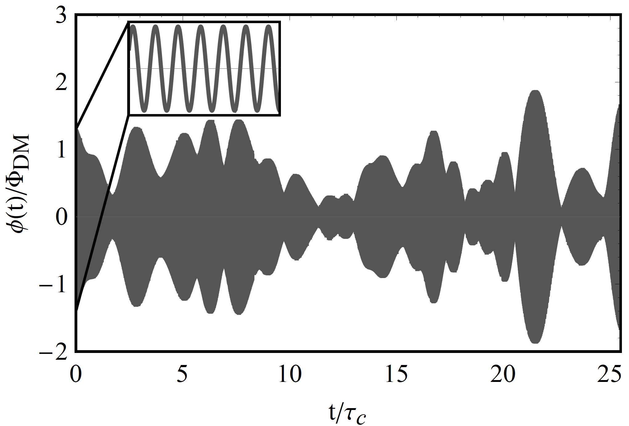
Figure 1: Simulated VULF based on the approach in Ref. Derevianko (2018) with field value $\phi(t)$ and time normalized by $\Phi_{{\rm{DM}}}$ and coherence time $\tau_{c}$ respectively. The inset plot displays the high-resolution coherent oscillation starting at $t=0$.

Figure 1 shows a simulated VULF field, illustrating the amplitude modulation present over several coherence times. At short time scales ($\ll\tau_{c}$) the field coherently oscillates at the Compton frequency, see the inset of Fig. 1, where the amplitude $\Phi_{0}$ is fixed at a single value sampled from its distribution. An unlucky experimentalist could even have near-zero field amplitudes during the course of their measurement.

On these short time scales the DM signal $s(t)$ exhibits a harmonic signature,

$$s(t)=\gamma\xi\phi(t)\approx\gamma\xi\Phi_{0}\cos(2\pi f_{\phi}t+\theta)\,,$$ (1)

where $\gamma$ is the coupling strength to a standard-model field and $\theta$ is an unknown phase. Details of the particular experiment are accounted for by the factor $\xi$. In this regime the amplitude $\Phi_{0}$ is unknown and yields a time-averaged energy density $\langle\phi(t)^{2}\rangle_{T\ll\tau_{c}}=\Phi_{0}^{2}/2$. However, for times much longer than $\tau_{c}$ the energy density approaches the ensemble average determined by $\langle\Phi_{0}^{2}\rangle=\Phi_{\mathrm{DM}}^{2}$. This field oscillation amplitude is estimated by assuming that the average energy density in the bosonic field is equal to the local DM energy density $\rho_{\mathrm{DM}}\approx 0.4\,{\rm{GeV/cm^{3}}}$, and thus $\Phi_{\mathrm{DM}}=\hbar(m_{\phi}c)^{-1}\sqrt{2\rho_{\mathrm{DM}}}$.

The oscillation amplitude sampled at a particular time for a duration $\ll\tau_{c}$ is not simply $\Phi_{\mathrm{DM}}$, but rather a random variable whose sampling probability is described by a distribution characterizing the stochastic nature of the VULF. Until recently, most experimental searches have been in the $m_{\phi}\gg 10^{-13}\,{\rm{eV}}$ regime with short coherence times $\tau_{c}\ll 1\,{\rm{day}}$. However, for smaller boson masses it becomes impractical to sample over many coherence times: for example, $\tau_{c}\gtrsim 1\,{\rm{year}}$ for $m_{\phi}\lesssim 10^{-16}\,{\rm{eV}}$. Assuming the value $\Phi_{0}=\Phi_{{\rm{DM}}}$ neglects the stochastic nature of the bosonic dark matter field Abel et al. (2017); Garcon et al. (2019); Wu et al. (2019); Terrano et al. (2019); Van Tilburg et al. (2015); Hees et al. (2016); Wcisło et al. (2018).

The net field $\phi(t)$ is a sum of different field modes with random phases. The oscillation amplitude, $\Phi_{0}$, results from the interference of these randomly phased oscillating fields. This can be visualized as arising from a random walk in the complex plane, described by a Rayleigh distribution Foster et al. (2018)

$$p({\Phi_{0}})={\frac{{2{\Phi_{0}}}}{{\Phi_{{\rm{DM}}}^{2}}}\exp\left({-\frac{{\Phi_{0}^{2}}}{{\Phi_{{\rm{DM}}}^{2}}}}\right)\,,}$$ (2)

analogous to that of chaotic (thermal) light Loudon (1983). This distribution implies that $\approx$ 63% of all amplitude realizations will be below the r.m.s. value $\Phi_{\mathrm{DM}}$. Equation (2) Foster et al. (2018) is typically represented in its exponential form Knirck et al. (2018) (see Supplementary Material), and is well sampled in the $T\gg\tau_{c}$ regime. However, this stochastic behavior should not be ignored in the opposite limit.

We refer to the conventional approach assuming $\Phi_{0}=\Phi_{{\rm{DM}}}$ as deterministic and approaches that account for the VULF amplitude fluctuations as stochastic. To compare these two approaches we choose a Bayesian framework and calculate the numerical factor affecting coupling constraints, allowing us to illustrate the effect on exclusion plots of previous deterministic constraints Abel et al. (2017); Garcon et al. (2019); Wu et al. (2019); Terrano et al. (2019); Van Tilburg et al. (2015); Hees et al. (2016); Wcisło et al. (2018). It is important to emphasize that different frameworks to interpret experimental data than presented here can change the magnitude of this numerical factor Protassov et al. (2002); Cowan et al. (2011); Conrad (2015); Tanabashi et al. (2018), see Supplementary Material for a detailed discussion. In any case, accounting for this stochastic nature will generically relax existing constraints as we show below.

Establishing constraints on coupling strength — We follow the Bayesian framework Gregory (2010) (see application to VULFs in Ref. Derevianko (2018)) to determine constraints on the coupling-strength parameter $\gamma$. Bayesian inference requires prior information on the parameter of interest to derive its respective posterior probability distribution, in contrast to purely likelihood-based inference methods. The central quantity of interest in our case is the posterior distribution for possible values of $\gamma$, derived from Bayes theorem,

$$p(\gamma|D,f_{\phi},\xi)=\mathcal{C} \int p(\gamma,\Phi_{0})\mathcal{L}(D|\gamma,\Phi_{0},f_{\phi},\xi)d\Phi_{0}\,.$$ (3)

The left-hand side of the equation is the posterior distribution for $\gamma$, where $D$ represents the data, and the Compton frequency $f_{\phi}$ is a model parameter. $\mathcal{C}$ is the normalization constant, and the likelihood $\mathcal{L}(\cdots)$ is the probability of obtaining the data $D$ given that the model and prior information, such as those provided by the SHM, are true. The integral on the right-hand side accounts for (marginalizes over) the unknown VULF amplitude $\Phi_{0}$, which we assume follows the Rayleigh distribution described by Eq. (2). For the choice of prior $p(\gamma,\Phi_{0})$ we use what is known as an objective prior Kass and Wasserman (1996): the Berger-Bernardo reference prior  Berger and Bernardo (1992). Results from Bayesian inference are sensitive to the choice of prior Berger and Bernardo (1992), and we find better agreement with frequentist based approaches when using an objective prior rather than a uniform prior $p(\gamma)=1$ (see Supplementary Material).

It is important to note that experiments searching for couplings of VULFs to fermion spins (axion “wind” searches) are sensitive not only to the amplitude of the bosonic filed but also to the relative velocity between the laboratory and the VULF, which stochastically varies on a time scale $\approx\tau_{c}$ Graham and Rajendran (2013). The signal due to the axion wind is proportional to the projection of this stochastically varying velocity onto the sensitive axis of the experiment. Accounting for the stochastic nature of the relative velocity increases the uncertainty of the derived coupling strength for a given measurement. Axion-wind experiments can also utilize the daily modulation of this projection, due to rotation of the Earth, to search for signals with an oscillation period much longer than the measurement time $T\ll 1/f_{\phi}$. The unknown initial phase $\theta$ of the VULF sets the amplitude of this daily oscillation and also needs to be marginalized over. We describe how we account for stochastic variations of velocity and daily modulation in the relevant experiments Abel et al. (2017); Garcon et al. (2019); Wu et al. (2019); Terrano et al. (2019) in the Supplementary Material and focus solely on the stochastic variations of the amplitude, $\Phi_{0}$, here.

Using the posterior distribution, $p(\gamma|D,f_{\phi},\xi)$, one can set constraints on the coupling strength $\gamma$. Such a constraint at the commonly employed 95% confidence level (CL), $\gamma_{95\%}$, is given by

$$\int_{0}^{\gamma_{95\%}}p(\gamma|D,f_{\phi},\xi)d\gamma=0.95\,.$$ (4)

The posteriors in both the deterministic and stochastic treatments are derived in the Supplementary Material. In short, the two posteriors differ due to the marginalization over $\Phi_{0}$ for the stochastic case, see the integral of Eq. (3). Assuming white noise of variance $\sigma^{2}$ and that the data are in terms of excess amplitude $A$ (observed Fourier amplitude divided by expected noise, an analog to the excess power statistic) we can derive the posterior for excess signal amplitude $A_{s}$. The posteriors are

$$p_{\mathrm{det}}(A_{s}|A)\propto p(A_{s})2A\exp\left(-A^{2}-A_{s}^{2}\right)I_{0}\left(2AA_{s}\right)\,,$$ (5)

$$p_{\mathrm{stoch}}(A_{s}|A)\propto p(A_{s})\frac{2A}{(1+A_{s}^{2})}\exp\left(-\frac{A^{2}}{1+A_{s}^{2}}\right)\,.$$ (6)

Here $A_{s}\equiv\gamma\times\xi\Phi_{\mathrm{DM}}\sqrt{N}/(2\sigma)$, $I_{0}(x)$ is the modified Bessel function of the first kind, and $p(A_{s})$ is effectively the prior on $\gamma$. In Fig. 2 we plot the normalized posteriors assuming $A$ at the 95% detection threshold $A^{dt}=\sqrt{-\ln{(1-0.95)}}$ and using Berger-Bernardo reference priors for $p(A_{s})$; we compare other choices of prior in the Supplementary Material. The derivation relies on the discrete Fourier transform for a uniform sampling grid of $N$ points and the assumptions of the uniform grid and white noise can be relaxed Derevianko (2018).

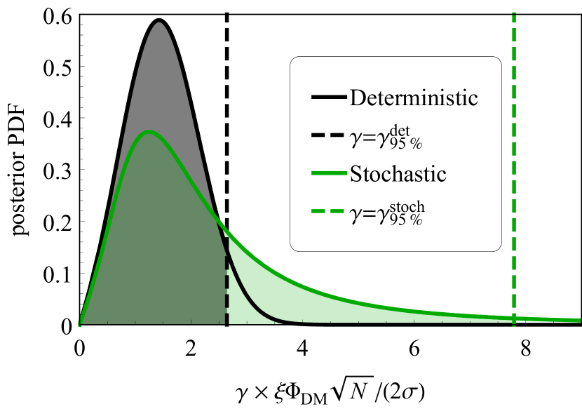
Figure 2: Posterior distributions for the coupling strength $\gamma$ in the deterministic and stochastic treatments, Eqs. (5) and (6) respectively. Due to the fat-tailed shape of the stochastic posterior one can clearly see the 95% limit is larger with $\gamma_{95\%}^{\mathrm{stoch}}/\gamma_{95\%}^{\mathrm{det}}\approx 3.0$. The assumed value of the data is at the 95% detection threshold $A^{dt}=\sqrt{-\ln{(1-0.95)}}$ (see text).

Examination of Eqs. (5), (6) and Fig. 2 reveals that the fat-tailed stochastic posterior is much broader than the Gaussian-like deterministic posterior. It is clear that for the stochastic posterior, the integration must extend considerably further into the tail, leading to larger values of $\gamma_{95\%}$ and thereby to weaker constraints, $\gamma_{95\%}^{\mathrm{stoch}}>\gamma_{95\%}^{\mathrm{det}}$. Explicit evaluation of Eq. (4) with the derived posteriors results in a relation between the constraints

$$\gamma_{95\%}^{\mathrm{stoch}}\approx 3.0\,\gamma_{95\%}^{\mathrm{det}}\,,$$ (7)

where the numerical value of the correction factor depends on CL and assumed value of $A$ (the factor increases for higher CL and decreases for smaller $A$).

This correction factor becomes $\approx 10$ when derived using a uniform prior, as discussed in the Supplementary Material. However, the result obtained with the uniform prior is not invariant under a change of variables (e.g. from excess amplitude to power). Additionally, using the objective prior yields better agreement with frequentist-based results of a factor $\approx 2.7$. For the pseudoscalar coupling, the additional stochastic parameters (field velocity and phase) increase this factor up to $\approx 8.4$ as shown in the Supplementary Material.

Ultralight DM candidates are theoretically well motivated and an increasing number of experiments are searching for them. Most of the experiments with published constraints thus far are haloscopes, sensitive to the local galactic DM and affected by Eq. (7). However, experiments that measure axions generated from a source, helioscopes or new-force searches, for example, do not fall under the assumptions made here. We illustrate how the existing constraints have been affected in Fig. 3 and provide more detailed exclusion plots for the axion-nucleon coupling $g_{aNN}$ Abel et al. (2017); Wu et al. (2019); Garcon et al. (2019); Vasilakis et al. (2009) and for dilaton couplings Hees et al. (2016); Van Tilburg et al. (2015); Wcisło et al. (2018) in the Supplementary Material.

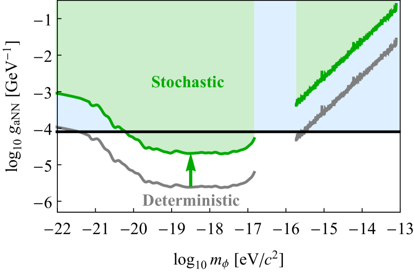
Figure 3: The modified constraint, green line, based on the stochastic approach compared to previous laboratory constraints, gray line, based on the deterministic approach for the axion-nucleon coupling strength $g_{aNN}$ Abel et al. (2017); Wu et al. (2019); Garcon et al. (2019); Vasilakis et al. (2009). The black line represents a constraint from a new-force search using a K-³He comagnetometer Vasilakis et al. (2009), unaffected by the local galactic properties of DM.

Figure 3 shows that a few previously published constraints for the axion-nucleon coupling Abel et al. (2017); Wu et al. (2019); Garcon et al. (2019) no longer constrain new parameter space with respect to the new force constraint at $\approx 10^{-4}$ GeV^-1 Vasilakis et al. (2009).

Conclusion – To interpret the results of an experiment searching for bosonic DM in the regime of measurement times smaller than the coherence time, stochastic properties of the net field must be taken into account. An accurate description accounts for the Rayleigh-distributed amplitude $\Phi_{0}$, where the variation is induced by the random phases of individual virialized fields. Accounting for this stochastic nature yields a correction factor of $\approx 2.7-10$, relaxing existing experimental bosonic DM constraints in this regime. In the event of a bosonic DM discovery, the stochastic properties of the field would result in increased uncertainty in the determination of coupling strength or local average energy density in this regime.

It is important to note that observational knowledge of the local distribution of DM can constrain stochastic behavior of the amplitude (energy density). The smallest features observed so far are on the order of $\approx 10$ pc Iocco et al. (2015) (corresponding to a $m_{\phi}\approx 10^{-21}$ eV coherence length), however the analysis in Ref. Iocco et al. (2015) performs radial averages which would remove the stochastic variation discussed in this paper.

Data Availability – All conclusions made in this paper can be reproduced using the information presented in the manuscript and/or Supplementary Material. Additional information is available upon reasonable request to the corresponding author. For access to the experimental data presented here please contact the corresponding authors of the respective papers.

Acknowledgments – We thank Eric Adelberger and William A. Terrano for pointing out the need to account for the unknown phase in the CASPEr-ZULF Comagnetometer analysis. We thank Kent Irwin, Marina Gil Sendra, and Martin Engler for helpful discussions and suggestions. We thank M. Zawada, N. A. Leefer, and A. Hees for providing raw data for the published deterministic constraints. We also thank Jelle Aalbers for helpful discussions and expert advice on the blueice inference framework. Jan Conrad appreciates the support by the Knut and Alice Wallenberg Foundation. This project has received funding from the European Research Council (ERC) under the European Unions Horizon 2020 research and innovation programme (grant agreement No 695405). We acknowledge the partial support of the U.S. National Science Foundation, the Simons and Heising-Simons Foundations, and the DFG Reinhart Koselleck project.

References

- Dimopoulos and Giudice (1996) S. Dimopoulos and G. F. Giudice, Physics Letters B 379, 105 (1996).
- Arkani-Hamed et al. (2000) N. Arkani-Hamed, L. Hall, D. Smith, and N. Weiner, Phys. Rev. D 62, 105002 (2000).
- Taylor and Veneziano (1988) T. R. Taylor and G. Veneziano, Physics Letters B 213, 450 (1988).
- Damour and Polyakov (1994) T. Damour and A. M. Polyakov, Nuclear Physics B 423, 532 (1994).
- Peccei and Quinn (1977a) R. D. Peccei and H. R. Quinn, Physical Review D (1977a), 10.1103/PhysRevD.16.1791.
- Peccei and Quinn (1977b) R. D. Peccei and H. R. Quinn, Physical Review Letters (1977b), 10.1103/PhysRevLett.38.1440.
- Weinberg (1978) S. Weinberg, Physical Review Letters 40, 223 (1978).
- Wilczek (1978) F. Wilczek, Physical Review Letters 40, 279 (1978).
- Graham et al. (2015) P. W. Graham, I. G. Irastorza, S. K. Lamoreaux, A. Lindner, and K. A. van Bibber, Annual Review of Nuclear and Particle Science 65, 485 (2015), arXiv:1602.00039v1 .
- Irastorza and Redondo (2018) I. G. Irastorza and J. Redondo, Progress in Particle and Nuclear Physics 102, 89 (2018).
- DePanfilis et al. (1987) S. DePanfilis, A. C. Melissinos, B. E. Moskowitz, J. T. Rogers, Y. K. Semertzidis, W. U. Wuensch, H. J. Halama, A. G. Prodell, W. B. Fowler, and F. A. Nezrick, Physical Review Letters 59, 839 (1987).
- Wuensch et al. (1989) W. U. Wuensch, S. De Panfilis-Wuensch, Y. K. Semertzidis, J. T. Rogers, A. C. Melissinos, H. J. Halama, B. E. Moskowitz, A. G. Prodell, W. B. Fowler, and F. A. Nezrick, Physical Review D 40, 3153 (1989).
- Hagmann et al. (1990) C. Hagmann, P. Sikivie, N. S. Sullivan, and D. B. Tanner, Physical Review D (1990), 10.1103/PhysRevD.42.1297.
- Asztalos et al. (2010) S. J. Asztalos, G. Carosi, C. Hagmann, D. Kinion, K. van Bibber, M. Hotz, L. J. Rosenberg, G. Rybka, J. Hoskins, J. Hwang, P. Sikivie, D. B. Tanner, R. Bradley, and J. Clarke, Physical Review Letters 104, 041301 (2010).
- Graham and Rajendran (2013) P. W. Graham and S. Rajendran, Physical Review D - Particles, Fields, Gravitation and Cosmology 88, 1 (2013), arXiv:arXiv:1306.6088v2 .
- Budker et al. (2014) D. Budker, P. W. Graham, M. Ledbetter, S. Rajendran, and A. O. Sushkov, Physical Review X 4, 021030 (2014), arXiv:1306.6089 .
- Brubaker et al. (2017) B. M. Brubaker, L. Zhong, S. K. Lamoreaux, K. W. Lehnert, and K. A. van Bibber, Physical Review D 96, 123008 (2017).
- Caldwell et al. (2017) A. Caldwell, G. Dvali, B. Majorovits, A. Millar, G. Raffelt, J. Redondo, O. Reimann, F. Simon, and F. Steffen, Physical Review Letters 118, 091801 (2017).
- Miller (2017) M. C. Miller, Nature 551, 36 (2017).
- Chung (2015) W. Chung, in Proceedings of Science (2015).
- Choi et al. (2017) J. Choi, H. Themann, M. J. Lee, B. R. Ko, and Y. K. Semertzidis, Physical Review D 96, 061102 (2017).
- McAllister et al. (2017) B. T. McAllister, G. Flower, E. N. Ivanov, M. Goryachev, J. Bourhill, and M. E. Tobar, Physics of the Dark Universe 18, 67 (2017).
- Alesini et al. (2017) D. Alesini, D. Babusci, D. Di Gioacchino, C. Gatti, G. Lamanna, and C. Ligi, (2017), arXiv:1707.06010 .
- Stadnik and Flambaum (2015) Y. V. Stadnik and V. V. Flambaum, Physical Review Letters 114, 161301 (2015).
- Grote and Stadnik (2019) H. Grote and Y. V. Stadnik, “Novel signatures of dark matter in laser-interferometric gravitational-wave detectors,” (2019), arXiv:1906.06193 .
- Marsh (2016) D. J. Marsh, Physics Reports 643, 1 (2016), arXiv:0610440 [astro-ph] .
- Marsh and Silk (2014) D. J. Marsh and J. Silk, Monthly Notices of the Royal Astronomical Society (2014), 10.1093/mnras/stt2079.
- Hu et al. (2000) W. Hu, R. Barkana, and A. Gruzinov, Physical Review Letters 85, 1158 (2000).
- Hui et al. (2017) L. Hui, J. P. Ostriker, S. Tremaine, and E. Witten, Physical Review D (2017), 10.1103/PhysRevD.95.043541, arXiv:1610.08297 .
- Arvanitaki et al. (2010) A. Arvanitaki, S. Dimopoulos, S. Dubovsky, N. Kaloper, and J. March-Russell, Physical Review D 81, 123530 (2010).
- Arvanitaki et al. (2015) A. Arvanitaki, J. Huang, and K. Van Tilburg, Phys. Rev. D 91, 015015 (2015).
- Abel et al. (2017) C. Abel, N. J. Ayres, G. Ban, G. Bison, K. Bodek, V. Bondar, M. Daum, M. Fairbairn, V. V. Flambaum, P. Geltenbort, et al., Physical Review X 7, 041034 (2017).
- Garcon et al. (2019) A. Garcon, J. W. Blanchard, G. P. Centers, N. L. Figueroa, P. W. Graham, D. F. Jackson Kimball, S. Rajendran, A. O. Sushkov, Y. V. Stadnik, A. Wickenbrock, T. Wu, and D. Budker, Science Advances 5, eaax4539 (2019), arXiv:1902.04644 .
- Wu et al. (2019) T. Wu, J. W. Blanchard, G. P. Centers, N. L. Figueroa, A. Garcon, P. W. Graham, D. F. J. Kimball, S. Rajendran, Y. V. Stadnik, A. O. Sushkov, A. Wickenbrock, and D. Budker, Physical Review Letters 122, 191302 (2019), arXiv:1901.10843 .
- Terrano et al. (2019) W. A. Terrano, E. G. Adelberger, C. A. Hagedorn, and B. R. Heckel, Physical Review Letters 122, 231301 (2019), arXiv:1902.04246 .
- Van Tilburg et al. (2015) K. Van Tilburg, N. Leefer, L. Bougas, and D. Budker, Physical Review Letters 115, 011802 (2015).
- Hees et al. (2016) A. Hees, J. Guéna, M. Abgrall, S. Bize, and P. Wolf, Physical Review Letters 117, 061301 (2016).
- Wcisło et al. (2018) P. Wcisło, P. Ablewski, K. Beloy, S. Bilicki, M. Bober, R. Brown, R. Fasano, R. Ciuryło, H. Hachisu, T. Ido, et al., Science Advances 4, eaau4869 (2018).
- Geraci and Derevianko (2016) A. A. Geraci and A. Derevianko, Phys. Rev. Lett. 117, 261301 (2016).
- Derevianko (2018) A. Derevianko, Physical Review A 97, 042506 (2018), arXiv:1605.09717 .
- Zwicky (1933) F. Zwicky, Published in Helvetica Physica Acta (1933), 10.1007/s10714-008-0707-4, arXiv:1711.01693 .
- Kuhlen et al. (2014) M. Kuhlen, A. Pillepich, J. Guedes, and P. Madau, The Astrophysical Journal 784, 161 (2014).
- Freese et al. (2013) K. Freese, M. Lisanti, and C. Savage, Reviews of Modern Physics 85, 1561 (2013), arXiv:1209.3339 .
- Diemand et al. (2008) J. Diemand, M. Kuhlen, P. Madau, M. Zemp, B. Moore, D. Potter, and J. Stadel, Nature 454, 735 (2008).
- Sikivie and Yang (2009) P. Sikivie and Q. Yang, Physical Review Letters 103, 111301 (2009), arXiv:0901.1106 .
- Davidson (2015) S. Davidson, Astroparticle Physics (2015), 10.1016/j.astropartphys.2014.12.007.
- Berges and Jaeckel (2015) J. Berges and J. Jaeckel, Physical Review D - Particles, Fields, Gravitation and Cosmology (2015), 10.1103/PhysRevD.91.025020.
- Jackson Kimball et al. (2018) D. F. Jackson Kimball, D. Budker, J. Eby, M. Pospelov, S. Pustelny, T. Scholtes, Y. V. Stadnik, A. Weis, and A. Wickenbrock, Physical Review D (2018), 10.1103/PhysRevD.97.043002.
- Khlopov et al. (1985) M. Y. Khlopov, B. A. Malomed, and Y. B. Zeldovich, Monthly Notices of the Royal Astronomical Society 215, 575 (1985).
- Knirck et al. (2018) S. Knirck, A. J. Millar, C. A. O’Hare, J. Redondo, and F. D. Steffen, Journal of Cosmology and Astroparticle Physics 2018, 051 (2018), arXiv:1806.05927 .
- Foster et al. (2018) J. W. Foster, N. L. Rodd, and B. R. Safdi, Physical Review D 97, 123006 (2018).
- Chan et al. (2018) J. H. H. Chan, H.-Y. Schive, T.-P. Woo, and T. Chiueh, Monthly Notices of the Royal Astronomical Society 478, 2686 (2018), arXiv:1712.01947 .
- Lin et al. (2018) S.-C. Lin, H.-Y. Schive, S.-K. Wong, and T. Chiueh, Physical Review D 97, 103523 (2018), arXiv:1801.02320 .
- Veltmaat et al. (2018) J. Veltmaat, J. C. Niemeyer, and B. Schwabe, Physical Review D 98, 043509 (2018), arXiv:1804.09647 .
- Schive et al. (2014) H. Y. Schive, T. Chiueh, and T. Broadhurst, Nature Physics 10, 496 (2014), arXiv:1406.6586 .
- Romano and Cornish (2017) J. D. Romano and N. J. Cornish, Living Reviews in Relativity 20, 1 (2017), arXiv:1608.06889 .
- Loudon (1983) R. Loudon, The Quantum Theory of Light, 2nd ed. (Oxford University Press, 1983).
- Protassov et al. (2002) R. Protassov, D. A. van Dyk, A. Connors, V. L. Kashyap, and A. Siemiginowska, The Astrophysical Journal 571, 545 (2002).
- Cowan et al. (2011) G. Cowan, K. Cranmer, E. Gross, and O. Vitells, The European Physical Journal C 71, 1 (2011).
- Conrad (2015) J. Conrad, “Statistical issues in astrophysical searches for particle dark matter,” (2015).
- Tanabashi et al. (2018) M. Tanabashi, K. Hagiwara, K. Hikasa, K. Nakamura, Y. Sumino, F. Takahashi, J. Tanaka, K. Agashe, G. Aielli, C. Amsler, et al., Physical Review D 98, 030001 (2018), arXiv:0601168 [astro-ph] .
- Gregory (2010) P. Gregory, Bayesian Logical Data Analysis for the Physical Sciences: A Comparative Approach with Mathematica Support (Cambridge University Press, 2010).
- Kass and Wasserman (1996) R. E. Kass and L. Wasserman, Journal of the American Statistical Association 91, 1343 (1996).
- Bernardo (1979) J. M. Bernardo, Journal of the Royal Statistical Society: Series B (Methodological) 41, 113 (1979).
- Berger and Bernardo (1992) J. O. Berger and J. M. Bernardo, Biometrika (1992), 10.2307/2337144.
- Vasilakis et al. (2009) G. Vasilakis, J. M. Brown, T. W. Kornack, and M. V. Romalis, Physical Review Letters 103, 261801 (2009).
- Iocco et al. (2015) F. Iocco, M. Pato, and G. Bertone, Nature Physics 11, 245 (2015), arXiv:1503.08784 .