Dynamical disentanglement in an analysis of oscillatory systems: an application to respiratory sinus arrhythmia

Abstract

We develop a technique for the multivariate data analysis of perturbed self-sustained oscillators. The approach is based on the reconstruction of the phase dynamics model from observations and on a subsequent exploration of this model. For the system, driven by several inputs, we suggest a dynamical disentanglement procedure, allowing us to reconstruct the variability of the system’s output that is due to a particular observed input, or, alternatively, to reconstruct the variability which is caused by all the inputs except for the observed one. We focus on the application of the method to the vagal component of the heart rate variability caused by a respiratory influence. We develop an algorithm that extracts purely respiratory-related variability, using a respiratory trace and times of R-peaks in the electrocardiogram. The algorithm can be applied to other systems where the observed bivariate data can be represented as a point process and a slow continuous signal, e.g. for the analysis of neuronal spiking.

I Introduction

One of the basic problems in the data analysis is to select or to eliminate a particular component of a given time series, e.g. to remove noise or a trend, or to single out an oscillation in a certain frequency band, etc. A whole variety of techniques has been designed to tackle this task by means of filtering in the frequency domain, smoothing in a running window, subtracting a fitted polynomial, and so on. Furthermore, a number of modern methods – principal component analysis, independent mode decomposition, empirical mode decomposition Fukunaga-90 ; Huang-98 ; Jolliffe-2002 ; Flandrin-04 ; Feldman-11 ; PhysRevE.92.032916 – represent a signal of interest as a sum of modes such that (at least) dominating modes are assumed to represent certain relevant dynamical processes. Correspondingly, some of these modes can be analyzed separately or, on the contrary, if they are considered as irrelevant, they can be subtracted from the original data, so that the cleansed signal can be further processed.

In this publication we elaborate on a technique for a dynamical disentanglement of different components, designed for the analysis of signals, generated by coupled oscillatory systems. The disentanglement task is illustrated in Fig. 1. We assume that a signal from an oscillatory unit, which is driven by an observed nearly periodic signal and by other, non-observed inputs is known (Fig. 1a). (We treat the unobserved input as some noise, although generally it may contain some regular components as well.) The technique is based on a reconstruction of the phase dynamics of the analyzed unit. The obtained equation is then used for generation of two new outputs. If only the observed input is used, i.e. the unobserved noise term is omitted, then the simulated equation yields a signal representing the dynamics of the noise-free system, i.e. the system driven by the observed input only (Fig. 1b). If, on the contrary, we eliminate from the equation the observed input, then the simulations yield the noise-induced output (Fig. 1c). This disentanglement procedure is neither the standard filtering (because the preserved and eliminated components can overlap in the frequency domain), nor the mode decomposition (because the sum of two disentangled outputs does not yield the original signal). Here we consider application of this approach to cardiac and respiratory data in humans. Our main oscillatory unit will be the cardiovascular system, and the observed input will be respiration. As the results of the analysis we will obtain two heart rate variability signals: one influenced purely by respiration, and one where the influence of respiration is excluded.

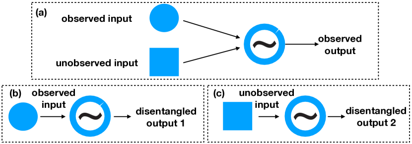
Figure 1: Schematic representation of the disentanglement procedure. (a): Original setup, where two inputs influence the oscillator. (b): Reconstruction of the “noise-free” dynamics. (c): reconstruction of the “signal-free” dynamics.

Understanding of the cardiac dynamics in terms of coupled oscillators goes back to the pioneering work by van der Pol and van der Mark van_der_Pol_van_der_Mark-28 . Within the last two decades this idea was widely used to address the interaction between the cardiovascular and respiratory systems with the aim to reveal and quantify synchronization between them and to infer directionality and strength of their coupling  Schaefer-Rosenblum-Kurths-Abel-98 ; Mrowka-Patzak-Rosenblum-00 ; PhysRevLett.85.4831 ; Rosenblum_et_al-02 ; Mrowka_et_al-03 ; Kralemann_et_al-13 ; Iatsenko_et_al-13 . Here we discuss how application of the coupled oscillators theory helps in the analysis of the main effect of the cardio-respiratory interaction, namely modulation of the heart rate by respiration, known for about a century as respiratory sinus arrhythmia (RSA) Eckberg-83 ; Berntson-Cacioppo-Quigley-93 ; Eckberg-03 ; Billman-11 ; Beauchaine-15 .

The separation and proper quantification of this respiratory component of heart rate variability (HRV) is of great importance for both fundamental physiological research and clinical medicine Lehofer1999 ; Moser1998 , due to the role vagal activity plays not only in cardiovascular, but also in inflammatory control Tracey2002 . The isolated immune system is over-reactive and self propagating by it’s nature. Germs or degraded cells in our body are detected by immune cells like macrophages floating in the interstitial space of the tissue. Macrophages detecting germ intruders produce inflammatory signals such as TNF-alpha and interleucine 1 Olofsson_et_al-12 , which attract other immune cells from nearby blood vessels. Without neuro-humoral control, the immune system would enter a dangerous state of generalized inflammation, well known as “sepsis” in clinical medicine.

To prevent this generalized reaction, vagal afferents (transmitting from periphery to brain) also carry receptors for these signal substances and transmit the information on inflammation location and strength to brain stem areas Andersson-Tracey-12 . After processing this information, vagal efferents (transmitting from brain to periphery) respond by release of acetylcholine at the location of the inflamed tissue Tracey2002 . Nicotinergic acetylcholine receptors have been identified on the surface of the macrophages, which down-regulate the cytocine production as a response to the cholinergic stimulation Rosas-Ballina-Tracey-09 , thereby reducing the attraction of additional inflammatory immune cells and down-regulating immune response. This inflammatory feedback loop prevents over-activity of the immune system enabling the brain to locally control the immune activity. Therefore, a reduction of the vagal tone, e.g., by different forms of stress, is suspected to be related to several chronic diseases induced by inflammation, including type 2 diabetes, ulceral colitis, Hashimoto’s thyreoiditis, and even cancer Nathan-Ding-2010 . Severe reductions of vagal tone has been observed in patients with these conditions Donchin_et_al-92 ; Moser2006 ; Das2011 ; Chow_et_al-14 . The action of sympathetic activity in this system is not as well-understood as vagal contribution at the moment. Therefore it is important to measure the vagal component separated from the other components. Linear separation by filtering the signal can improve the estimation of pure vagal tone, but under certain conditions may fail to do so, when the respiratory frequency approaches other meta-cardiac cycles deriving from sympathetic origin, like the blood pressure rhythm of 0.1 Hz.

In our previous publications Kralemann_et_al-13 ; Topcu_et_al-18 we applied the dynamical disentanglement approach to the analysis of RSA in heart rate variability records. In these publications we used simultaneous measurements of electrocardiogram (ECG) and respiratory activity in order to reconstruct the equation of the phase dynamics of the cardiac oscillator. Next, we exploited this equation for a decomposition of the heartbeat intervals series into respiratory-related and non-respiratory-related components. This decomposition can be used as a general preprocessing tool for quantification of respiratory related heart rate variability and, in particular, opens a new way to address the clinically important problem of RSA quantification.

However, the results of Refs. Kralemann_et_al-13 ; Topcu_et_al-18 can be considered only as a proof of principle, because they were obtained using a continuous phase of the cardiac oscillators. Determination of such a phase requires very clean high-quality measurements and a tedious preprocessing. Here we suggest an easy-to-implement practical algorithm for achieving the same goal using the information about timing of the R-peaks only. The latter are well-defined events within each cycle of cardiac activity and they can be readily obtained with any standard equipment. From the viewpoint of data analysis, we deal with a relatively slow smooth signal (respiration), the phase of which can be easily estimated, e.g. by means of the Hilbert transform, and a point process (R-peaks) with a frequency about 3 times higher. Point processes frequently appear in neuronscience, and, thus, our algorithm can be also helpful in the analysis of neural data, e.g. of spiking neurons affected by a slow observed continuous force.

II Dynamical disentanglement based on the phase dynamics modeling

Our general goal is to identify dynamical properties of an oscillatory system, related to different influences, from the observations of its behavior in a complex noisy environment. For example, one can be interested in the following questions: what would be the dynamics of the system if it were noise-free? Or, how the statistical properties of the oscillation would change if one of the external forces were switched off? We address these and similar problems using the phase dynamics theory, see, e.g. Winfree-67 ; Kuramoto-84 ; Pikovsky-Rosenblum-Kurths-01 .

Consider a limit cycle oscillator, weakly perturbed by regular or stochastic known forces $\eta_{k}(t)$, $k=1,2,\ldots$. Then, according to the theory, in the first approximation in amplitude of these forces, the phase dynamics obeys

$$\dot{\varphi}=\omega+\sum_{k}Q_{k}[\varphi,\eta_{k}(t)]+\zeta(t)\;.$$ (1)

Here $\varphi(t)$ and $\omega$ are the phase and the natural frequency of the system, and $Q_{k}$ are the coupling functions; they quantify response of the oscillator to the corresponding perturbations. The random term $\zeta(t)$ accounts for intrinsic fluctuations of the system parameters. Notice that the same equation describes dynamics of weakly chaotic systems; in this case $\zeta(t)$ reflects effects of chaotic amplitude variations. In the second-order approximation in the force amplitudes, one expects appearance of triple terms like $Q_{12}[\varphi,\eta_{1},\eta_{2}]$, etc Kralemann-Pikovsky-Rosenblum-11 ; Kralemann-Pikovsky-Rosenblum-14 , but these effects will be neglected below.

Let us suppose first that Eq. (1) is known. Then, if we are interested in properties of the purely deterministic phase dynamics, we can solve numerically Eq. (1) without the noise term $\zeta(t)$ (we speak on the deterministic dynamics here because the forces $\eta_{k}(t)$ are known (recordered) functions of time, though they must not be completely regular). If the task is to analyze the response of the oscillator to a particular external force, e.g. $\eta_{1}(t)$, then we omit in Eq. (1) the terms $\xi(t)=\sum_{k>1}Q_{k}[\varphi,\eta_{k}(t)]+\zeta(t)$, simulate the equation

$$\dot{\varphi}=\omega+Q_{1}[\varphi,\eta_{1}(t)]\;,$$ (2)

and analyze the obtained result according to a particular problem in question. This approach was used in Rosenblum-Pikovsky-18 for reconstructing the Arnold tongue of a noise-free oscillator (with strictly regular force $\eta_{1}(t)$) from a measurement of noisy system (where in addition to $\eta_{1}(t)$ also pure noise $\zeta(t)$ is present). Alternatively, if we are interested in the effects of the random component $\zeta(t)$, e.g. in properties of phase diffusion, then we have to omit the deterministic perturbations and solve numerically

$$\dot{\varphi}=\omega+\xi(t)\;.$$ (3)

In this way we achieve the desired dynamical disentanglement. Below we apply this general idea to the analysis of cardio-respiratory interaction.

III Disentanglement of the heart rate variability

In Ref. Kralemann_et_al-13 we used the measurements of ECG and respiratory flow from healthy adults in order to reconstruct the model of cardiac phase dynamics in the form

$$\dot{\varphi}=\omega+Q(\varphi,\psi)+\xi(t)\;,$$ (4)

where $\varphi$ and $\psi$ correspond to the instantaneous phases of the cardiac and the respiratory rhythms, respectively. This equation is a particular case of Eq. (1), with $\eta_{1}(t)$ corresponding to the respiration dynamics. Since the latter is a rhythmical process with a well-defined phase $\psi$, we write the corresponding coupling function as a function of two phases, $Q_{1}(\varphi,\eta_{1}(t))=Q(\varphi,\psi)$, while the contribution of other, unobserved, perturbations and of intrinsic fluctuations is combined in the rest term $\xi=\sum_{k>1}Q_{k}(\varphi,\eta_{k}(t))+\zeta(t)$. Practically, $Q(\varphi,\psi)$ as a function of two variables was constructed on a $64\times 64$ equidistant grid on a domain $(0,2\pi)\times(0,2\pi)$.

Notice that determination of the respiratory phase $\psi$ is simple: since the respiratory signal looks like a modulated and slightly distorted sine-wave, its phase can be easily estimated, e.g., by means of the Hilbert transform. On the contrary, the ECG signal has a quite complicated form and computations of its phase represent a nontrivial stand-alone problem, see Ref. Kralemann_et_al-13 : here one needs very high-quality data, and its processing is technically quite demanding. This fact motivates a development of techniques operating only with point processes, namely with instants of the R-peaks, corresponding to the peak of depolarization of the ventricles of the human heart. These events can be easily detected and therefore are commonly used in the analysis of HRV. Since these peaks appear once per heartbeat cycle, their continuous phase $\varphi$ without loss of generality can be set to zero.

First, we discuss how the disentanglement of the HRV can be performed if both continuous phases $\varphi(t)$ and $\psi(t)$ are available Kralemann_et_al-13 . For this goal we notice that, for a given time series $\varphi(t)$ and $\psi(t)$, the coupling function in Eq. (4) can be also interpreted as a time series $Q[\varphi(t),\psi(t)]=Q(t)$. Correspondingly, knowledge of time series $\dot{\varphi}(t)$ and $Q(t)$ yields the rest term $\xi(t)=\dot{\varphi}-Q$. Having all these time series, we easily construct the new disentangled ones. These are the respiratory-related (R) and the non-respiratory related (NR) components of the instantaneous cardiac frequency, denoted as $\dot{\varphi}^{(R)}$ and $\dot{\varphi}^{(NR)}$, and obtained according to equations

$$\dot{\varphi}^{(R)}=\omega+Q(\varphi^{(R)},\psi)\quad\text{and}\quad\dot{\varphi}^{(NR)}=\omega+\xi(t)\;.$$ (5)

Notice that this is not a simple decomposition because $\dot{\varphi}(t)\neq\dot{\varphi}^{(R)}(t)+\dot{\varphi}^{(NR)}(t)$. In Ref. Kralemann_et_al-13 we have demonstrated that power spectrum of $\dot{\varphi}^{(R)}$ nicely describes the spectral peaks corresponding to the frequency of respiration and to the side-bands of the heart rate.

In the subsequent study Topcu_et_al-18 , we extended this idea and generated artificial sequences of heartbeat events (R-peaks) according to the conditions $\varphi^{(R)}(t_{k}^{(R)})=2\pi k$ and $\varphi^{(NR)}(t_{k}^{(NR)})=2\pi k$, $k=1,2,\ldots$, where the phases were obtained via numerical integration of differential Eqs. (5). The point process $t_{k}^{(R)}$ represents instants of the heart beats as they would appear if there were no other perturbations to the cardiac oscillator, except for the respiration, while $t_{k}^{(NR)}$ represents the heart rate variability due to internal fluctuations and external non-respiratory rhythms, e.g. blood pressure and blood perfusion rhythms. It has been suggested that described decomposition into respiratory-related (R-HRV) and non-respiratory-related (NR-HRV) components shall be used as a generic preprocessing technique prior to a quantification of the RSA in clinical practice. This suggestion has been supported by computation of different measures of RSA from the original series of inter-beat intervals as well as from respiratory-related intervals $T^{(R)}=t_{k+1}^{(R)}-t_{k}^{(R)}$, see Topcu_et_al-18 for details. Notice that our approach is intrinsically nonlinear, in contrast to ad hoc techniques used for the same purpose, like adaptive filtering and least-mean-square fitting of power spectra Widjaja_et_al-14 ; Kuo-Kuo-16 .

Summarizing, the disentanglement of the instantaneous cardiac frequency into R-HRV and NR-HRV components can be easily implemented, provided the continuous phases $\varphi,\psi$ are known. However, as already mentioned, computation of the instantaneous cardiac phase $\varphi$ requires high-quality measurements, visual inspection of the data, extensive preprocessing, and is currently solved by ad hoc, not automated, techniques only. On the other hand, determination of the R-peaks is a standard task and can be easily accomplished. Therefore, development of an disentanglement algorithm for the case when one observable, e.g. respiration, is continuous and appropriate for the phase estimation, and the other one, e.g. heartbeats, is a point process, represents an important unsolved problem. Below we present an approximate solution of this problem.

IV Dynamical disentanglement for the point process data

Our starting point is the description of the cardio-respiratory phase dynamics in form of Eq. (4). We assume that the respiratory phase $\psi$ is obtained from the respiratory time series and that the instants $t_{k}$, when the R-peaks appear in the electrocardiogram, are determined. The cardiac phase at these instants is $\varphi(t_{k})=2\pi k$. Let the inter-beat intervals be denoted as $T_{k}=t_{k+1}-t_{k}$. Then, assuming weakness of the coupling, $\parallel Q\parallel\ll\omega$, where $\parallel\cdot\parallel$ denotes the norm of the function, and keeping in Eq. (4) only the deterministic term, we write in the first approximation

$$\int_{t_{k}}^{t_{k+1}}\mathrm{d}t=T_{k}=\int_{0}^{2\pi}\frac{d\varphi}{\omega+Q(\varphi,\psi)}\approx\frac{2\pi}{\omega}-\frac{1}{\omega^{2}}\int_{0}^{2\pi}Q(\varphi,\psi)\mathrm{d}\varphi\;.$$ (6)

Next, since the respiration is much slower than the heart rate, we assume that within the inter-beat interval $T_{k}$, the phase $\psi$ grows linearly in time with the frequency $\omega^{(r)}_{k}$, i.e. $\psi(t)=\psi_{k}+\omega^{(r)}_{k}(t-t_{k})$, where $\psi_{k}=\psi(t_{k})$. Then the integral in Eq. (6) can be approximated as

$$-\omega^{-2}\int_{0}^{2\pi}Q(\varphi,\psi)\mathrm{d}\varphi=-\omega^{-2}\int_{0}^{T_{k}}Q[\varphi(t),\psi(t)]\mathrm{d}t\approx F(\psi_{k},\omega^{(r)}_{k})\;.$$

Taking for simplicity $\omega^{(r)}_{k}=\dot{\psi}(t_{k})=\dot{\psi}_{k}$ (corrections to this expresion, due to slowness of the respiratory phase, appear in the higher orders) and denoting $T=2\pi/\omega$, we obtain

$$T_{k}=T+F(\psi_{k},\dot{\psi}_{k})+\chi_{k}\;,$$ (7)

where $F(\psi_{k},\dot{\psi}_{k})$ can be understood as a discrete version of the coupling function (we denote it as the coupling map) and the rest term $\chi_{k}$ is the random component. Equation (7) can be considered as a direct discrete analogue of continuous Eq. (4).

Introducing the mean respiratory frequency $\bar{\omega}=\langle\omega^{(r)}_{k}\rangle_{k}=\langle\dot{\psi}_{k}\rangle_{k}$ and expressing $F(\psi_{k},\omega_{k})$ as a Taylor-Fourier series, we finally write

$$T_{k}\approx T+\sum_{n=1}^{N_{F}}\left\{\left[\sum_{m=0}^{N_{T}-1}a_{n,m}(\dot{\psi}_{k}-\bar{\omega})^{m}\right]\cos(n\psi_{k})+\left[\sum_{m=0}^{N_{T}-1}b_{n,m}(\dot{\psi}_{k}-\bar{\omega})^{m}\right]\sin(n\psi_{k})\right\}\;.$$ (8)

Here $N_{F}$ and $N_{T}$ are the orders of the Fourier and Taylor series, respectively. For a sufficiently long series of inter-beat intervals $T_{k}$, Eqs. (8) can be considered as an overdetermined linear system for unknown parameters $T,a_{n,m}$, $b_{n,m}$. This system can be easily solved, e.g., by mean squares minimization.

Thus, the suggested algorithm yields a discrete dynamical model (7) for the inter-beat intervals. Now this model can be used for the dynamical disentanglement. In order to construct the respiratory-related component we first take $t_{1}^{(R)}=t_{1}$. Then, substituting $\psi_{1}$, $\dot{\psi}_{1}$ in (8) we obtain $T_{1}^{(R)}$ and $t_{2}^{(R)}=t_{1}^{(R)}+T_{1}^{(R)}$. Next, we compute $\psi(t_{2}^{(R)})$, $\dot{\psi}(t_{2}^{(R)})$ and use the model (8) to obtain $T_{2}^{(R)}$ and $t_{3}^{(R)}$, and so on . For the construction of the non-respiratory-related component we also start by assigning $t_{1}^{(NR)}=t_{1}$ and then proceed as follows. Let already determined $t_{l}^{(NR)}$ fulfill $t_{k}<t_{l}^{(NR)}<t_{k+1}$. For $t_{k}$ and $t_{k+1}$ we compute the rest term of the model (8) (effective noise), i.e. the difference between the true $T_{k}$, $T_{k+1}$ and their value predicted by Eq. (8); these terms are $\chi_{k}$ and $\chi_{k+1}$. Then, using linear interpolation to find the effective noise at $t_{l}^{(NR)}$, we obtain

$$t_{l+1}^{(NR)}=t_{l}^{(NR)}+T+\chi_{k}+\frac{\chi_{k+1}-\chi_{k}}{t_{k+1}-t_{k}}(t_{l}^{(NR)}-t_{k})\;.$$ (9)

The R-HRV component can be further used for an improved quantification of the RSA, while the NR-HRV time series can be exploited for the analysis of the other sources of the heart rate variability.

V Testing the approach on model data

First we verify our approach using artificially generated data with known properties. For this goal we use a simple phase model (4), where the coupling function $Q(\varphi,\psi)$ is written in the Winfree form, i.e. as a product of the phase sensitivity function, or phase response curve (PRC), $Z(\varphi)$, and forcing function $I(\psi)$. Thus, introducing explicitly the coupling strength parameter $\varepsilon$, we write

$$\dot{\varphi}=\omega+\varepsilon Z(\varphi)I(\psi)+\xi(t)\;.$$ (10)

Functions $Z(\varphi)$, $I(\psi)$ are modeled by Fourier series of order 15 and 4, respectively, see Fig. 2, in such a way that they resemble experimentally obtained curves, cf. Kralemann_et_al-13 .

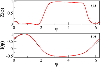
Figure 2: Model phase response curve of the cardiac oscillator (a) and model respiratory force (b) are shown by bold red lines. Dashed lines in both panels indicate the corresponding curves obtained in experiments, cf. Kralemann_et_al-13 .

Instantaneous frequency of respiration was modeled as $\dot{\psi}=\omega_{r}+\mu\nu$, where $\nu$ is an Ornstein-Uhlenbeck process, $\dot{\nu}=-\gamma_{r}\nu+\eta_{1}$. The random term $\xi$ is given by the weighted sum of two components, i.e. of a low-pass and of a band-pass filtered noise: $\xi=\lambda_{1}\zeta_{1}+\lambda_{2}\zeta_{2}$, where $\dot{\zeta}_{1}=-\gamma\zeta_{1}+\eta_{2}$ and $\ddot{\zeta}_{2}+\alpha\dot{\zeta}_{2}+\omega_{bp}^{2}\zeta_{2}=\eta_{3}$. Here $\eta_{k}$ are independent Gaussian white noises with zero mean: $\langle\eta_{k}(t)\eta_{j}(t^{\prime})\rangle=\delta_{kj}\delta(t-t^{\prime})$.

Solving stochastic differential Eq. (10), we generate the artificial series of R-peaks. Without loss of generality, we say that these peaks occur when phase $\varphi$ attains a multiple of $2\pi$. Thus, we obtain a point process $t_{k}$ such that $\varphi(t_{k})=2\pi k$. Correspondingly, we introduce series of RR-intervals $T_{k}=t_{k+1}-t_{k}$. Similarly, solving the deterministic part of Eq. (10), i.e.

$$\dot{\varphi}^{(R)}=\omega+\varepsilon Z(\varphi)I(\psi)\;,$$ (11)

we generate a series of respiratory-related R-peaks, $t_{k}^{(R)}$ and corresponding intervals $T_{k}^{(R)}$ . Finally, the non-respiratory related R-peaks, $t_{k}^{(NR)}$ and the interbeat intervals $T_{k}^{(NR)}$ are obtained via solution of

$$\dot{\varphi}^{(NR)}=\omega+\xi(t)\;.$$ (12)

Thus, the data used for the disentanglement are: the times of R-peaks, $t_{k}$, and the respiratory phase and the frequency, $\psi(t)$ and $\dot{\psi}(t)$, and in particular $\psi(t_{k})=\psi_{k}$, and $\dot{\psi}(t_{k})=\dot{\psi}_{k}$. Notice that in this test two latter series are obtained from equations, while in fact respiratory phase and frequency should be estimated from data, what certainly will introduce an additional error. The respiratory-related and the non-respiratory-related components obtained via dynamic disentanglement, shall be compared with $t_{k}^{(R)}$ and $t_{k}^{(NR)}$, respectively.

Here we illustrate the model data and the disentanglement results for the following values of the parameters: $\omega=2\pi$, $\omega_{r}=2$, $\varepsilon=0.1$, $\omega_{bp}=1.08\pi$, $\alpha=0.1$, $\gamma_{r}=0.1$, $\mu=0.02$, $\lambda_{1}=0.03$, $\lambda_{2}=0.02$,. The records used for the subsequent analysis contained about $10^{4}$ interbeat intervals, which correspond to about $2.5$ hours of natural heart beat. The model data are illustrated in Fig. 3. Here we show a short epoch of the artificially generated sequences of RR-intervals.

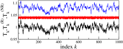
Figure 3: A short epoch of the model data. From bottom to top: artificial sequence of interbeat interval, its respiratory-related, and non-respiratory related components. The latter two curves are shifted upwards for visibility.

Figure 4 presents the respiratory-related component, extracted with the help of our algorithm with $N_{F}=8$, $N_{T}=2$, compared to the true one, i.e. generated by the model. Figure 5 illustrate the results of the disentanglement in the frequency domain. Namely, here we present spectra of point processes (Bartlett measure) Bartlett-63 . As expected, spectral peaks induced by respiration are enhanced in the R-component and suppressed in the NR-component.

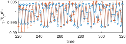
Figure 4: True (blue circles) and recovered (red crosses) respiratory components of the HRV. The first one is generated by the model, while the second one is obtained from the point process by means of constructing the coupling map (8).

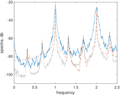
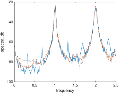
Figure 5: Illustration of the disentanglement in the frequency domain. Here we show the spectra of the point processes for the respiratory-related component (left panel) and for the NR component (right panel). Blue solid line shows the spectrum of model-generated series of instances of R-peaks $t_{k}$; red dashed curves show the spectrum of the model-generated series $t_{k}^{(R)}$, $t_{k}^{(NR)}$, while the black dotted curves present the spectra of the R- and NR-components obtained from $t_{k}$ via disentanglement.

We conclude the presentation of the technique by discussing a characterization of the quality of disentanglement. First we notice that, as it follows from Eqs. (10,11,12) and as is expected for a disentanglement of independent components, $\text{Var}(\dot{\varphi})=\text{Var}(\dot{\varphi}^{(R)})+\text{Var}(\dot{\varphi}^{(NR)})$, where the variance is defined as $\text{Var}(x(t))=\langle(x-\langle x\rangle)^{2}\rangle$, $\langle(\cdot)\rangle=T_{\Sigma}^{-1}\int_{0}^{T_{\Sigma}}(\cdot)\mathrm{d}t$, and $T_{\Sigma}$ is the time interval over which the averaging is performed. We expect that a similar relation for variances obtained from the interval series $T_{k}$, $T_{k}^{(R)}$, $T_{k}^{(NR)}$ shall be also valid, at least approximately. To compute the variance of the phase derivative for a point process, we consider the phase linearly growing between the events, so that $\dot{\varphi}(t)=2\pi/T_{k}$ for $t_{k}\leq t\leq t_{k+1}$, $k=1,\ldots,N$. Then, for the variance we obtain

$$\sigma^{2}=\frac{4\pi^{2}}{T_{\Sigma}}\sum_{k=1}^{N}\left(\frac{1}{T_{k}}-\frac{N}{T_{\Sigma}}\right)^{2}T_{k}\;,$$ (13)

where $T_{\Sigma}=\sum_{k}T_{k}$, and similarly for the respiratory-related and the non-respiratory-related components. We checked, for different $N_{F},N_{T}$, that indeed $(\sigma^{2}_{R}+\sigma^{2}_{NR})/\sigma^{2}\approx 1$ (for $N_{T}\leq 3$ the worst case was $0.97$).

VI An application to human cardio-respiratory data

Now we apply our algorithm to real data. For this goal we analyzed 26 multivariate records of ECG and respiration, registered in 17 healthy adults in supine position at rest, see Kralemann_et_al-13 ; Gallasch_et_al-96 ; Gallasch_et_al-97 for a detailed description of the subjects, experimental protocol, and measurement equipment. Since continuous phases $\varphi(t),\psi(t)$ obtained in Kralemann_et_al-13 are available, we compare the approximate disentanglement performed with the help of Eqs. (7,8) with the results obtained for continuous phases.

In order to quantify the quality of the disentanglement we compute $(\sigma^{2}_{R}+\sigma^{2}_{NR})/\sigma^{2}$ for all subjects with the help of Eq. (13). The results shown in Figs. 6 indicate that our algorithm works quite well.

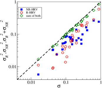
Figure 6: Quality of the point-process based disentanglement for cardio-respiratory data from healthy subjects. Here we plot, for each experimental record, variances of the respiratory and non-respiratory-related components and their sum vs. variance of the original sequence of R-peaks. As expected for uncorrelated components, the sum of variances of disentangled processes is very close to the variance of original data.

Here we used $N_{F}=8$, $N_{T}=1$; for $N_{T}>1$ the quality of the disentanglement was bad, probably because our point process series are quite short (about 400 heartbeats).

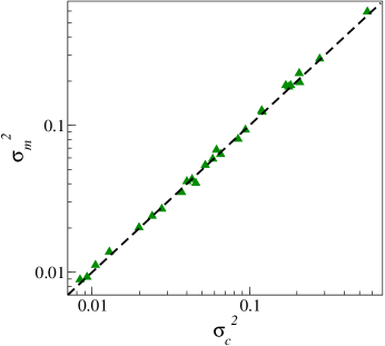
Figure 7: The efficiency of the map-based disentanglement is confirmed by plotting the variance $\sigma_{m}^{2}$ of the map-cleansed respiratory-related component vs. the variance $\sigma_{c}^{2}$ of the continuously-cleansed respiratory-related component.

Next, we compare the variance obtained from map-cleansed intervals with the variance for continuously-cleansed data, see Fig. 7. Both are in a good agreement.

An example of disentanglement (for a particular recording, data set 3) is shown in Fig. 8.

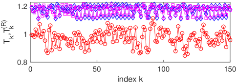
Figure 8: Original series of RR-intervals, $T_{k}$ (in seconds), of a healthy subject (red circles) and its respiratory-related component, $T_{k}^{(R)}$, obtained either via continuous cleansing (blue diamonds) or by map cleansing (magenta squares). Both cleansed time series are shifted upwards for visibility.

Here we show the original series of RR-intervals and the two cleansed data sets, one obtained via the disentanglement with the continuous phase and one obtained using only the R-peaks. For better visibility, two cleansed data sets are shifted upwards by $0.2$s, their overlap indicates that the discrete dynamical disentanglement works well.

VII Conclusion

To summarize, we have presented a general approach that allows us, by means of the reconstruction of the dynamics of a driven oscillator, to predict its “virtual dynamics” in which some of its inputs are cut off. The described disentanglement procedure differs from known mode decomposition algorithms, because it operates not with the given time series, but with a reconstructed phase dynamics equation. In this paper we focused on the extension of the dynamical disentanglement to the case when the output of the investigated oscillator is a sequence of events (a point process), so that its instantaneous phase can be hardly estimated, while the observed input is relatively slow and smooth process, suitable for the phase estimation. We applied this approach to analyze human heart rate variability, where the available time series are a respiration signal and heart beat events. More precisely, we disentangled the respiratory-related variability, known to be mediated by the vagus nerve only, from that due to other sources. Using both model data as well as instantaneous phases derived from an electrocardiogram, we have shown that our approximate procedure yields quite good results.

The developed technique can find applications in physiological as well as clinical studies. Indeed, quantification of different components of HRV is already an important diagnostic and prognostic tool in cardiology Moser1994 ; Malik_et_al-96 . Several circulatory diseases show a strong difference in prognosis depending on vagal activity. As already mentioned, the simple spectral methods applied to RR interval analysis in many clinical studies is not performing well in separating vagal respiratory and other components of HRV. Since our technique provides respiratory-related variability cleansed from the effect of noise and other, unobserved rhythms, quantification of RSA and hence vagal tone from disentangled data is more precise. The separation of respiratory and non-respiratory components is physiologically and clinically especially important in slow breathing ($<0.12$ Hz), where the vagal RSA intermixes with slower rhythms like blood pressure rhythm, which derive from sympathetic and vagal components. Under such conditions the two components of autonomic nervous system activity cannot be separated with linear models Cysarz_et_al-04 .

In Ref. Topcu_et_al-18 we compared performance of different RSA measures applied to original and cleansed series. However, there the disentanglement was performed using instantaneous continuous phases. Now we show that the practical algorithm that operates not with a continuous ECG, but only with R-peaks, provides nearly the same results. This finding opens a way to practical use. We anticipate that the developed technique can be also used in neuroscience, e.g. for analysis of spiking of sensory neurons in response to a slowly varying stimulus.

As a subject of future research, we mention a case of more than one observed input. Theoretically, it is not so difficult to perform the phase dynamics reconstruction for multivariate data; however, data requirements increase essential so that reconstruction of a network of more than 3 oscillators becomes unfeasible, see Kralemann-Pikovsky-Rosenblum-14 . Another interesting extension would be the case of non-oscillatory inputs, when parameterization of these inputs by a phase does not work. A possible solution for both problems might be reconstruction of the phase dynamics in the Winfree form, i.e. when the coupling function can be presented as a product of the phase response curve and of the driving signal, cf. Eq. (10).

MR, MM, and AP acknowledge financial support from the European Union’s Horizon 2020 research and innovation programme under the Marie Sklodowska-Curie Grant Agreement No. 642563 (COSMOS). Development of methods presented in Section 4 was supported by the Russian Science Foundation under Grant No. 17-12-01534.

References

- (1) Fukunaga K. 1990 Introduction to Statistical Pattern Recognition. Amsterdam: Elsevier.
- (2) Huang NE, Shen Z, Long SR, Wu MC, Shih HH, Zheng Q, Yen NC, Tung CC, Liu HH. 1998 The empirical mode decomposition and the Hilbert spectrum for nonlinear and non-stationary time series analysis. Proceedings of the Royal Society of London Series A 454, 903–998.
- (3) Jolliffe I. 2002 Principal Component Analysis. Berlin: Springer.
- (4) Flandrin P, Rillingas a filter bank. IEEE Signal Processing Lett. 11, 112–114.
- (5) Feldman M. 2011 Hilbert Transform Applications in Mechanical Vibration. UK: Wiley.
- (6) Iatsenko D, McClintock PVE, Stefanovska A. 2015 Nonlinear mode decomposition: A noise-robust, adaptive decomposition method. Phys. Rev. E 92, 032916.
- (7) van der Pol B, van der Mark. 1928 The heartbeat considered as a relaxation oscillation and an electrical model of the heart. Phil. Mag. 6, 763–775.
- (8) Schäfer C, Rosenblum MG, Kurths J, Abel HH. 1998 Heartbeat synchronized with ventilation. Nature 392, 239–240.
- (9) Mrowka R, Patzak A, Rosenblum MG. 2000 Qantitative analysis of cardiorespiratory synchronization in infants. Int. J. of Bifurcation and Chaos 10, 2479–2488.
- (10) Stefanovska A, Haken H, McClintock PVE, Hožič M, Bajrović F, Ribarič S. 2000 Reversible transitions between synchronization states of the cardiorespiratory system. Phys. Rev. Lett. 85, 4831–4834.
- (11) Rosenblum MG, Cimponeriu L, Bezerianos A, Patzak A, Mrowka R. 2002 Identification of coupling direction: Application to cardiorespiratory interaction. Phys. Rev. E 65, 041909.
- (12) Mrowka R, Cimponeriu L, Patzak A, Rosenblum M. 2003 Directionality of coupling of physiological subsystems - age related changes of cardiorespiratory interaction during different sleep stages in babies. American J. of Physiology Regul. Comp. Integr. Physiol. 145, R1395–R1401.
- (13) Kralemann B, Frühwirth M, Pikovsky A, Rosenblum M, Kenner T, Schaefer J, Moser M. 2013 In vivo cardiac phase response curve elucidates human respiratory heart rate variability. Nature Communications 4, 2418.
- (14) Iatsenko D, Bernjak A, Stankovski T, Shiogai Y, Jane OLP, Clarkson PBM, McClintock PVE, Stefanovska A. 2013 Evolution of cardiorespiratory interactions with age. Philosophical Transactions of the Royal Society of London A 371.
- (15) Eckberg DL. 1983 Human sinus arrhythmia as an index of vagal cardiac outflow. J. Appl. Physiol. 54, 961–966.
- (16) Berntson GG, Cacioppo JT, Quigley KS. 1993 Respiratory sinus arrhythmia: Autonomic origins, physiological mechanisms, and psychological implications. Psychophysiology 30, 183–196.
- (17) Eckberg DL. 2003 The human respiratory gate. The Journal of physiology 548(Pt 2), 339–352.
- (18) Billman G. 2011 Heart rate variability – a historical perspective. Front Physiol. 2, 86.
- (19) Beauchaine TP. 2015 Respiratory sinus arrhythmia: A transdiagnostic biomarker of emotion dysregulation and psychopathology. Current opinion in psychology 3, 43–47.
- (20) Lehofer M, Moser M, Hoehn-Saric R, McLeod D, Hildebrandt G, Egner S, Steinbrenner B, Liebmann P, Zapotoczky HG. 1999 Influence of age on the parasympatholytic property of tricyclic antidepressants. Psychiatry Research 85, 199–207.
- (21) Moser M, Lehofer M, Hoehn-Saric R, McLeod DR, Hildebrandt G, Steinbrenner B, Voica M, Liebmann P, Zapotoczky HG. 1998 Increased heart rate in depressed subjects in spite of unchanged autonomic balance? Journal of Affective Disorders 48, 115–124.
- (22) Tracey KJ. 2002 The inflammatory reflex. Nature 420, 853–9.
- (23) Olofsson P, Rosas-Ballina M, Levine Y, Tracey K. 2012 Rethinking inflammation: neural circuits in the regulation of immunity. Immunol Rev 248, 188–204.
- (24) Andersson U, Tracey K. 2012 Neural reflexes in inflammation and immunity. J. Exp. Med. 209, 1057–1068.
- (25) Rosas-Ballina M, Tracey K. 2009 Cholinergic control of inflammation. J. Intern. Med. 265, 663–679.
- (26) Nathan C, Ding A. 2010 Nonresolving inflammation. Cell 140, 871–882.
- (27) Donchin Y, Constantini S, Szold A, Byrne EA, Porges SW. 1992 Cardiac vagal tone predicts outcome in neurosurgical patients. Crit. Care Med. 20, 942.
- (28) Moser M, Frühwirth M, Penter R, Winker R. 2006 Why life oscillates – from topographical towards a functional chronobiology. Cancer Cause Control 17, 591–599.
- (29) Das UN. 2011 Can vagus nerve stimulation halt or ameliorate rheumatoid arthritis and lupus? Lipids in Health and Disease 10, 19.
- (30) Chow E, Iqbal A, Bernjak A, Ajjan R, Heller SR. 2014 Effect of hypoglycaemia on thrombosis and inflammation in patients with type 2 diabetes. Lancet 383, S35.
- (31) Ç Topçu, Frühwirth M, Moser M, Rosenblum M, Pikovsky A. 2018 Disentangling respiratory sinus arrhythmia in heart rate variability records. Physiological Measurements 39, 054002.
- (32) Winfree AT. 1967 Biological rhythms and the behavior of populations of coupled oscillators. J. Theor. Biol. 16, 15.
- (33) Kuramoto Y. 1984 Chemical Oscillations, Waves and Turbulence. Berlin: Springer.
- (34) Pikovsky A, Rosenblum M, Kurths J. 2001 Synchronization. A Universal Concept in Nonlinear Sciences. Cambridge: Cambridge University Press.
- (35) Kralemann B, Pikovsky A, Rosenblum M. 2011 Reconstructing phase dynamics of oscillator networks. Chaos 21, 025104.
- (36) Kralemann B, Pikovsky A, Rosenblum M. 2014 Reconstructing effective phase connectivity of oscillator networks from observations. New Journal of Physics 16, 085013.
- (37) Rosenblum M, Pikovsky A. 2018 Efficient determination of synchronization domains from observations of asynchronous dynamics. Chaos 28, 106301.
- (38) For integration we used the Euler scheme; for initial conditions both and we set to zero at the instant of the first R-peak in the original data set. Since the coupling function is given on a grid, spline interpolation was used to compute for arbitrary .
- (39) Widjaja D, Caicedo A, Vlemincx E, Van Diest I, Van Huffel S. 2014 Separation of respiratory influences from the tachogram: A methodological evaluation. PLOS ONE 9, 1–11.
- (40) Kuo J, Kuo CD. 2016 Decomposition of heart rate variability spectrum into a power-law function and a residual spectrum. Front. Cardiovasc. Med. 3, 16.
- (41) For a high-resolution measurement phase and frequency of respiration are given as a time series with a small time step. Therefore, their values at can be obtained, e.g. by linear interpolation between two closest data points.
- (42) Notice that although Eq. (11) represents a deterministic part of Eq. (10), it remains a stochastic equation due to presence in the respiratory phase of an Ornstein-Uhlenbeck process component.
- (43) Bartlett M. 1963 The spectral analysis of point processes. J. R. Statist. Soc. Ser. B 29, 264–296.
- (44) Gallasch E, Rafolt D, Moser M, Hindinger J, Eder H, Wiesspeiner G, Kenner T. 1996 Instrumentation for assessment of tremor, skin vibrations, and cardiovascular variables in MIR space missions. IEEE Trans. Biomed. Eng. 43, 328–333.
- (45) Gallasch E, Moser M, Kozlovskaya I, Kenner T, Noordergraaf A. 1997 Effects of an eight-day space flight on microvibration and physiological tremor. Amer. J Physiol, Regul Integr Card 273, R86–R92.
- (46) This study was performed with a high-grade equipment especially developed for RR variability measurements at sampling rate 1000 Hz and resolution 16 bit, with shielded ECG cables. Notice that HRV measurements in medicine often do not meet such standards. Low data sampling rates ( Hz) and digital resolution ( bit) of commercial ECG equipment, built not for precise RR interval sampling but rather for low frequency ECG shape evaluation, introduce artificial jitter and digitizing noise detrimental for precise variability determination.
- (47) Moser M, Lehofer M, Sedminek A, Lux M, Zapotoczky HG, Kenner T, Noordergraaf A. 1994 Heart rate variability as a prognostic tool in cardiology. a contribution to the problem from a theoretical point of view. Circulation 90, 1078–1082.
- (48) Malik M, Bigger JT, Camm J, Kleiger RE, Malliani A, Moss AJ, Schwartz PJ. 1996 Heart rate variability: standards of measurement, physiological interpretation, and clinical use. Eur. Heart J. 17, 354–381.
- (49) Cysarz D, von Bonin D, Lackner H, Heusser P, Moser M, Bettermann H. 2004 Oscillations of heart rate and respiration synchronize during poetry recitation. Amer J Physiol - Heart Circ Phys 287, H579–H587.