On the instability tongues of the Hill equation
coupled with a conservative nonlinear oscillator

We study the asymptotics for the lengths $L_{N}(q)$ of the instability tongues of Hill equations that arise as iso-energetic linearization of two coupled oscillators around a single-mode periodic orbit. We show that for small energies, i.e. $q\rightarrow 0$, the instability tongues have the same behavior that occurs in the case of the Mathieu equation: $L_{N}(q)=O(q^{N})$. The result follows from a theorem which fully characterizes the class of Hill equations with the same asymptotic behavior. In addition, in some significant cases we characterize the shape of the instability tongues for small energies. Motivation of the paper stems from recent mathematical works on the theory of suspension bridges.

Keywords: Hill equation, Mathieu equation, instability tongues, coupled oscillators, coexistence

Mathematics Subject Classification: Primary: 34B30; Secondary: 37C75, 34C15

1 Introduction

We consider a class of parameterized Hill equations of the following type,

$$z^{\prime\prime}(t)+(\beta+g(u(t,q)))z(t)=0,$$ (1.1)

in which $\beta$ represents the spectral parameter, and the periodic coefficient depends (through the real analytic function g) on the solution $u=u(t,q)$ of an initial-value problem for a nonlinear conservative second order differential equation,

$$u^{\prime\prime}(t)+4u(t)+f(u(t))=0,\qquad u(0)=q,\quad u^{\prime}(0)=0.$$ (1.2)

In 1.2, $q$ is a real parameter, and the function $f$ is assumed to be real analytic in a neighborhood of $0$, with $f(x)=O(x^{2})$, $x\rightarrow 0$. Under this assumption, if $q$ is sufficiently small, the solution $u(t,q)$ is periodic with period $T(q)$. We shall refer to the period of the Hill equation 1.1 as $T(q)$, although in some cases the fundamental period of $g(u(t,q))$ could be a fraction of $T(q)$.

We are interested in certain asymptotic properties of the instability region of equation 1.1, which is the set of pairs of parameters $(q,\beta)$ such that all solutions of 1.1 are unbounded. According to the basic theory of the Hill equation [29][ch. II, Th. 2.1], [14], [ch. 2, Th. 2.3.1] for any admissible fixed value of $q$, the instability set in the $\beta$-axis is the union of an unbounded interval $(-\infty,\beta^{+}_{0}(q))$ with a countable family of, possibly empty, open intervals $I_{N}$, $N=1,2,\dots$, whose endpoints $\beta^{\pm}_{N}(q)$ are the $T(q)$-periodic eigenvalues for even $N$, or the $T(q)$-anti-periodic eigenvalues for odd $N$. When $\beta$ lies in the interior of the complementary set all solutions are bounded. As functions of $q$, the curves $\beta=\beta^{\pm}_{N}(q)$ form in the plane $(q,\beta)$ the boundaries of the so-called instability tongues (resonance tongues, Arnold’s tongues) of the Hill equation. These tongues stem and bifurcate from a sequence of points on the $\beta$-axis corresponding to the double eigenvalues $\beta^{+}_{N}(0)=\beta^{-}_{N}(0)=N^{2}$. Our main concern is the asymptotic behavior of $\beta^{\pm}_{N}(q)$ as $q\rightarrow 0$. We consider two types of problems:

• The order of tangency of $\beta^{\pm}_{N}(q)$ as $q\rightarrow 0$, that is the decay rate to zero of the signed length of the instability tongues $L_{N}(q)=\beta^{+}_{N}(q)-\beta^{-}_{N}(q)$.

• The shape of the instability tongues for small values of $q$. We shall distinguish between “trumpet shaped” tongues, containing a segment of the horizontal line $\beta=\beta_{N}(0)$, and “horn shaped” ones, whose intersection with the horizontal line $\beta=\beta_{N}(0)$ is empty for small $q$ (see Fig. 2 in Section 4).

We postpone motivations and results on problem (II) to Section 4. Problem (I) is classical in the standard theory of the Hill equation with two parameters. For instance, if we set $f(u)\equiv 0$ in 1.2 and $g(u)=u$, equation 1.1 reduces to the Mathieu equation $z^{\prime\prime}+(\beta+q\cos(2t))z=0$, for which the asymptotic length is known to be $L_{N}(q)=C_{N}q^{N}+O(q^{N+1})$, with precise determination of the coefficient $C_{N}\neq 0$, see [22, 28]. For the standard two-parameters Hill equation,

$$z^{\prime\prime}+(\beta+q\phi(t))z=0,$$ (1.3)

where $\phi$ is a general $L^{2}$ and $\pi$-periodic function, a classical result of Erdélyi [15] states that no better estimate than $L_{N}(q)=O(q)$ can be expected. In the case when $\phi(t)$ is a trigonometric polynomial of the form

$$\phi(t)=\sum_{j=1}^{s}a_{j}\cos(2jt),$$

Levy and Keller [28] (see also [4] for a different approach) proved that the length of the $N$-th resonance interval is at most $C_{N}q^{r}$, where $r$ is the integer part of $N/s$, and presented explicit formulas for $C_{N}$ when $N$ is a multiple of $s$ (see also [23], and [37] for interesting extensions to a generalized Ince equation). For the similar, and partly related, problem of the asymptotics of $L_{N}$ as $N\rightarrow\infty$, we refer to [6, 2].

In this paper we prove the following theorem which shows that, for every equation 1.1 coupled with 1.2, the instability tongues have at least the same order of tangency of the Mathieu equation, that is $L_{N}(q)=O(q^{N})$ as $q\rightarrow 0$.

Theorem 1.1.

Assume that the functions $f$, $g$ are real analytic in a neighborhood of the origin, with $f(x)=O(x^{2})$ as $x\rightarrow 0$. Then, for every $\;N\in\mathbb{N}$, there exists a (possibly vanishing) constant $C_{N}$, such that

$(A)$ $\qquad\qquad L_{N}(q)=C_{N}q^{N}+O(q^{N+1})\quad$ as $q\rightarrow 0$ .

It is not a simple task to compute the coefficient $C_{N}$, but we shall provide a recursive formula in Appendix A showing that $C_{N}$ is a polynomial of degree $N$ in the derivatives of $f$ and $g$ up to order $N$. We are unable to provide a uniform bound on the rest $L_{N}(q)-C_{N}q^{N}$ in terms of $f$, $g$ and $N$.

We stress the fact that $C_{N}$ is possibly vanishing because the coupled system 1.1–1.2 includes the classical Lamé equation corresponding, in our notations, to $f(u)=-6\,u^{2}$, and $g(u)=-m(m+1)u$, $m\in\mathbb{N}$. In this case, Ince [25] in 1940 showed that only finitely many, precisely $m$, instability intervals (thus tongues) fail to vanish. Equivalently, for all but $2m+1$ eigenvalues, there exist two linearly independent periodic eigenfunctions (coexistence). We shall briefly discuss this subject in Section 2.3 and Appendix B.

In order to prove Theorem 1.1, we need to rescale the time variable and the spectral parameter so that equation 1.1 reduces to a Hill equation whose periodic coefficient has fixed period $\pi$ and depends analytically on the parameter $q$:

$$z^{\prime\prime}+(\lambda+G(t,q))z=0.$$ (1.4)

Once this is done, the theorem is a consequence of the following characterization of the periodic coefficients $G(t,q)$ in 1.4 for which the asymptotic relation $(A)$ holds true.

Theorem 1.2.

Assume that $G(t,q)$ is an even $\pi$-periodic function, depending analytically on the parameter $q$ in a neighborhood of $0$. Then the lengths of the instability tongues of equation 1.4 satisfy the asymptotic estimate $(A)$, if and only if $\,G(t,q)$ admits the following power expansion,

$$G(t,q)=\sum_{n=1}^{\infty}G_{n}(t)q^{n},$$ (1.5)

in which the time coefficients are trigonometric polynomials of degree $2n$; that is,

$$G_{n}(t)=\sum_{k=0}^{n}G_{k,n}\cos(2kt),\qquad G_{k,n}\in\mathbb{R}.$$ (1.6)

In Theorem 1.2 we emphasize the inverse result that, as far as we know, is new even in the standard case $G(t,q)=q\phi(t)$, when it simply states that if the instability tongues of 1.3 satisfy (A), then either $\phi\equiv 0$ or 1.3 is the Mathieu equation. For this reason we take the liberty of naming generalized Mathieu equation, any Hill equation whose periodic coefficient admits an expansion such as 1.5–1.6.

A Hill equation such as 1.1 arises quite naturally in physical applications as the variational equation of periodic solutions in Hamiltonian systems with two degrees of freedom. A typical example is provided by a two-mode conservative system of oscillators that, for a given regular potential energy function $\Psi$, writes as follows,

$$u^{\prime\prime}(t)+\frac{\partial}{\partial u}\Psi(u(t),z(t))=0,$$ (1.7)

$$z^{\prime\prime}(t)+\frac{\partial}{\partial z}\Psi(u(t),z(t))=0.$$ (1.8)

If we assume the existence of a periodic single-mode motion, i.e. a periodic solution of 1.7–1.8 in which one component, say $u$, is periodic and the other vanishes, the active mode $u=u(t,q)$ can be seen as parameterized by its initial value $u(0)=q$ in the following way,

$$u^{\prime\prime}(t)+\frac{\partial}{\partial u}\Psi(u(t),0)=0,\qquad u(0)=q,\;u^{\prime}(0)=0.$$

The linearization at a fixed energy level (iso-energetic linearization) of the system 1.7–1.8 around the periodic orbit $(u(\cdot,q),0)$ yields the Hill equation,

$$z^{\prime\prime}(t)+\frac{\partial^{2}}{\partial z^{2}}\Psi(u(t),0)\,z(t)=0,$$

whose analysis, according to Floquet’s theory, determines the linearized stability or instability of the single-mode periodic motion. Thus the results in this paper are relevant for the parametric stability/instability analysis of the system 1.7–1.8 in the case when the energy of the coupled oscillators system is small. Here we consider $\beta=\frac{\partial^{2}}{\partial z^{2}}\Psi(0,0)$ as a parameter, $\frac{\partial^{2}}{\partial u^{2}}\Psi(0,0)=4$ (possibly after a suitable rescaling of time), $\frac{\partial}{\partial u}\Psi(u(t),0)=4u+f(u)$, $\frac{\partial^{2}}{\partial z^{2}}\Psi(u,0)=\beta+g(u)$.

The main motivation for starting the study of problems (I) and (II) is the analysis of parametric torsional instability for some recent suspension bridge models, where a finite dimensional projection of the phase space reduces the stability analysis at small energies of the model to the stability of a Hill equation such as 1.1. We refer the reader to Gazzola’s book [19], to the papers [8, 9, 3, 10, 17], and to our previous works [30, 31]. Other interesting applications arise in the study of the stability of nonlinear modes in some beam equations [18] or string equations [12, 11]. In the latter case, we must observe that the eigenvalue problem takes a different form: $\,z^{\prime\prime}+\beta(u+g(u))z=0$. Our results, in particular Theorem 1.1, extend to this form as well but in order to avoid redundancy of quite similar reasonings we do not include the proof.

The plan of the paper is the following: In Section 2, after introducing the problem in the context of analytic perturbation theory, we prove Theorem 1.2. The direct part is an adaptation of the argument in [28], whereas the converse makes use of a new inductive argument. In Section 3 we deal with our main result (Theorem 1.1) whose proof is, after rescaling, merely a verification of the assumptions of Theorem 1.2; in addition to a few complementary results we briefly recall the issue of the existence of finitely many tongues (coexistence). In Section 4 we discuss the shape of the instability tongues depending on the first coefficients in the expansions of $f$ and $g$. Some examples that are relevant to the theory of suspended bridges are examined in Section 5, and some situations are shown in which only finitely many tongues do not vanish; some are well-known while others are novel.

We include two appendices: Appendix A describes a recursive formula for the computation of $C_{N}$; Appendix B elaborates on a few transformations of the Lamé equation relevant for this work.

2 The generalized Mathieu Equation

In the first part of this section we consider the Hill equation 1.4, and the if part of Theorem 1.2. The inverse result will be proved in the second part of this section. The proof of the direct result is a variation and a simplification of an argument in [28]. The inverse proof uses a new, although simple, inductive procedure. Before proceeding with the proofs, we point out some general issues on the analytic perturbation problem we are addressing.

The periodic eigenvalue problem for the Hill equation 1.4 is a regular perturbation problem and may be cast in Kato’s abstract framework [26]. We assume that $G(\cdot,q)$ is $\pi$-periodic as a function of $t$, and is analytic in a neighborhood of $q=0$ as a function of $q$, with values in $L^{\infty}([0,\pi])$, i.e.

$$G(t,q)=\sum_{n=1}^{\infty}q^{n}G_{n}(t),\qquad\limsup_{n\rightarrow\infty}\|G_{n}\|_{\infty}^{1/n}<\infty.$$ (2.1)

To avoid distinction among periodic (even eigenvalue numbers) and anti-periodic (odd eigenvalue numbers) eigenfunctions, we assume as reference space the Hilbert space $H=L^{2}([-\pi,\pi])$, in which we consider the family of self-adjoint operators with discrete spectrum,

$$A(q)=-\frac{{\rm d}^{2}}{{\rm d}t^{2}}-\sum_{n=1}^{\infty}q^{n}G_{n},$$

with boundary conditions $z(-\pi)=z(\pi)$, $z^{\prime}(-\pi)=z^{\prime}(\pi)$. The Hilbert space $H$ may be decomposed according to $H=H^{+}\oplus H^{-}$, where $H^{\pm}$ denotes the subspace of even ($+$) functions, and odd ($-$) functions, that is

$$H^{+}=\mathop{\rm span}\{\cos kt:\,k\geq 0\},\quad H^{-}=\mathop{\rm span}\{\sin kt:\,k\geq 1\}.$$

Consequently, with obvious notation, we have $A(q)=A(q)^{+}\oplus A(q)^{-}$, so that the doubly degenerate eigenvalues $\lambda_{N}(0)=N^{2}$ turn out to be simple in $H^{\pm}$. Owing to the Rellich–Kato perturbation theorem (see e.g. [35]), every perturbed eigenvalue $\lambda^{\pm}_{N}(q)$ in $H^{\pm}$ depends analytically on $q$. We shall write the power series

$$\lambda^{\pm}_{N}(q)=N^{2}+\sum_{n=1}^{\infty}\Lambda_{n}^{\pm}(N)\,q^{n},$$ (2.2)

whose convergence radius $r_{N}$ can be estimated by Kato’s resolvent method: a lower bound for $r_{N}$ is given by the solution of the following equation (see [26, ch. II, §3]),

$$\sum_{n=1}^{\infty}r_{N}^{n}\|G_{n}\|_{\infty}=d_{N}/2,$$

where $d_{N}$ is the isolation distance of $\lambda_{N}(0)=\lambda_{N}^{\pm}(0)$, i.e. $d_{N}=N^{2}-(N-1)^{2}$.

From now on in this section, to avoid proliferation of indices, we omit the dependence on the eigenvalue number $N$, which we consider as fixed. We denote by $Z^{\pm}(t,q)$ the even ($+$) and odd ($-$) normalized (see below 2.6) eigenfunction corresponding to $\lambda^{\pm}_{N}$, whose power series expansion is given by

$$Z^{\pm}(t,q)=\sum_{n=0}^{\infty}q^{n}z^{\pm}_{n}(t).$$ (2.3)

If we plug the power series expansions 2.2, 2.3 into the equation 1.4, we get the following recursive sequence of differential equations,

$$z_{0}^{\prime\prime}+N^{2}z_{0}=0,$$ (2.4)

$$z_{n}^{\prime\prime}+N^{2}z_{n}+\sum_{s=1}^{n}\Lambda_{s}z_{n-s}+\sum_{s=1}^{n}G_{s}(t)z_{n-s}=0\qquad n\geq 1.$$ (2.5)

The $2\pi$-periodic solutions to 2.4–2.5 are not unique, unless we assume an additional constraint, such as the following,

$$\frac{1}{2\pi}\int_{-\pi}^{\pi}Z^{+}(t,q)\cos(Nt){\rm d}t=\frac{1}{2\pi i}\int_{-\pi}^{\pi}Z^{-}(t,q)\sin(Nt){\rm d}t=1.$$ (2.6)

2.1 Proof of Theorem 1.2: Direct problem

Here we assume that all coefficients $G_{n}$ are even $\pi$-periodic trigonometric polynomials of degree $2n$ such as in 1.6, and prove the property (A). The proof is divided into two steps: first we consider the Fourier expansion of each $z^{\pm}_{n}$, and write down recursive formulas for $\Lambda_{n}^{\pm}$, $z^{\pm}_{n}$; the rest of the proof relies mainly on a finite propagation speed of disturbances property of the system 2.10–2.11, which can be expressed either by the law of enlargement of supports or by the dual concept of domain of dependence, and is contained in three Lemmas; the last one, Lemma 2.3, shows that for $N\geq 1$ the order of tangency of $\lambda^{\pm}_{N}(q)$ at $q=0$ is at least $N-1$, that is $\Lambda_{n}^{+}(N)=\Lambda_{n}^{-}(N)$ in the expansion 2.2, for $n\leq N-1$. Of course this is equivalent to the asymptotic estimate (A) with $C_{N}=\Lambda_{N}^{+}(N)-\Lambda_{N}^{-}(N)$.

The Fourier expansion of each $z^{\pm}_{n}$ is:

$$z_{n}^{\pm}(t)=\sum_{k=-\infty}^{\infty}z_{k,n}^{\pm}e^{ikt},\qquad z_{-k,n}^{\pm}=\pm z_{k,n}^{\pm},$$ (2.7)

where the first component of the pair of indices $(k,n)\in\mathbb{Z}\times\mathbb{N}$ refers to frequency, the latter to the power of $q$, We note that, owing to 2.3, 2.6, and 2.7, we get the initial conditions at level $n=0$,

$$z_{k,0}^{\pm}=\delta_{k,N}\pm\delta_{k,-N},$$ (2.8)

and the fact that the $N$-th Fourier coefficient of $z_{n}$ is zero for $n\geq 1$, that is

$$z_{\pm N,n}^{\pm}=0,\qquad n\geq 1.$$ (2.9)

By substituting 2.7 in 2.5, we obtain the following recursive system for $z^{\pm}_{k,n}$, and $\Lambda_{n}^{\pm}$ ,

$$(N^{2}-k^{2})z_{k,n} = -\frac{1}{2}\sum_{s=1}^{n}\sum_{i=0}^{s}G_{i,s}(z_{k-2i,n-s}+z_{k+2i,n-s})-\sum_{s=1}^{n}\Lambda_{s}z_{k,n-s},$$ (2.10)

$$\Lambda_{n} = -\frac{1}{2}\sum_{s=1}^{n}\sum_{i=0}^{s}G_{i,s}\left(z_{N-2i,n-s}+z_{N+2i,n-s}\right).$$ (2.11)

The second equation 2.11 is obtained either by taking the scalar product of 2.5 with $e^{iNt}$ or by setting $k=N$ in 2.10. We note that the symmetry relations $z^{\pm}_{k,n}=\pm z_{k,n}^{\pm}$ are satisfied, since the system 2.10–2.11 is invariant under the transformation $k\mapsto-k$, and in the same way, one could get an equation equivalent to 2.11 by setting $k=-N$ in 2.10.

As in [28], we need the following lemmas on the vanishing coefficients of system 2.10–2.11.

Lemma 2.1.

The frequency index $k$ of non vanishing coefficients must have the same parity of $N$, that is $z_{k,n}^{\pm}=0$ for odd $k-N$. The indices of non vanishing coefficients are contained in the union of two forward cones:

$$S_{N}=\{(k,n)\in\mathbb{Z}\times\mathbb{N}:\,|k-N|\leq 2n\}\cup\{(k,n)\in\mathbb{Z}\times\mathbb{N}:\,|k+N|\leq 2n\}.$$

that is $z_{k,n}^{\pm}=0$, if $(k,n)$ belongs to the complementary set of $S_{N}$.

Proof.

The assertion on the parity of $k-N$ is easily proved by induction, but it is obvious if we think that for even/odd $N$, $z_{n}^{\pm}$ is a periodic/anti-periodic function. The other assertion is proved by induction on $n$. For $n=0$ the assertion is true by the initial conditions 2.8. Assume that it is true up to the level $n-1$, that is $z_{h,m}^{\pm}=0$, if $(h,m)\notin S_{N}$, and $m\leq n-1$. We remark that, for a given pair of indices $(k,n)\in\mathbb{Z}\times\mathbb{N}$, all the indices of $z_{k-2i,n-s}$, $z_{k+2i,n-s}$, $z_{k,n-s}$ in formula 2.10 belong to the following backward cone:

$$C_{\mathbf{k,n}}=\{(h,j)\in\mathbb{Z}\times\mathbb{N}:|k-h|\leq 2(n-j)\}\setminus\{(k,n)\}.$$ (2.12)

By a simple but cumbersome check, we have that if the vertex $(k,n)$ of $C_{\mathbf{k,n}}$ does not belong to $S_{N}$, then $C_{\mathbf{k,n}}\cap S_{N}=\emptyset$, and $j<n$ if $(h,j)\in C_{\mathbf{k,n}}$. Thus we get $z_{k,n}=0$, if $(k,n)\notin S_{N}$.

∎

Lemma 2.2.

The domain of dependence of $\Lambda_{n}^{\pm}$ is the backward cone $C_{\mathbf{N,n}}$, as defined in 2.12. The domain of dependence of $z^{\pm}_{k,n}$ is the backward cone $C_{\mathbf{k,n}}$. This means that the value of $z^{\pm}_{k,n}$ is not influenced by any $z_{h,j}^{\pm}$ if $(h,j)\notin C_{\mathbf{k,n}}.$

Proof.

The assertion on the domain of dependence of $\Lambda_{n}^{\pm}$ is verified by direct inspection of the indices in 2.11. Let us verify the assertion on the cone of $z^{\pm}_{k,n}$. As we noted in the proof of Lemma 2.1, every index of the $z$’s appearing in 2.10 belongs to $C_{\mathbf{k,n}}$. We need to take care of the domains of dependence of the terms $\Lambda_{s}^{\pm}$, with $s\leq n$, appearing in formula 2.10. We assume for the moment $k\geq 0$. The case $k=N$ is obvious. If $|k-N|=2h>0$, we remark that, owing to Lemma 2.1, the summation $\sum_{s=1}^{n}\Lambda_{s}^{\pm}z_{k,n-s}^{\pm}$ does not extended up to $n$. Indeed we have $z_{k,0}^{\pm}=z_{k,1}^{\pm}=\dots=z_{k,h-1}^{\pm}=0$, since their indices do not belong to the support set $S_{N}$, as it seen by the inequality $|k-N|=2h>2(n-s)$, $s>n-h$. Therefore summation can be replaced by (intended to vanish if $h\geq n$),

$$\sum_{s=1}^{n-h}\Lambda_{s}^{\pm}z_{k,n-s}^{\pm},\qquad 2h=|k-N|.$$ (2.13)

Since $C_{N,s}\subset C_{N,j}$ if $s\leq j$, the largest cone of dependence of the terms $\Lambda_{s}$ in 2.13 is $C_{\mathbf{N,n-h}}$ corresponding to the largest index $n-h$. By definition of $h$, $2h=|N-k|\leq 2|n-(n-h)|=2h$, thus its vertex $(N,n-h)$ belongs to $C_{k,n}$. It follows that the whole cone is contained in $C_{k,n}$. This proves the assertion on the dependence cone of $z_{k,n}^{\pm}$, if $k\geq 0$. The case $k<0$ reduces to the previous one by symmetry, since $z_{-k,n}^{\pm}=\pm z_{k,n}^{\pm}$ ∎

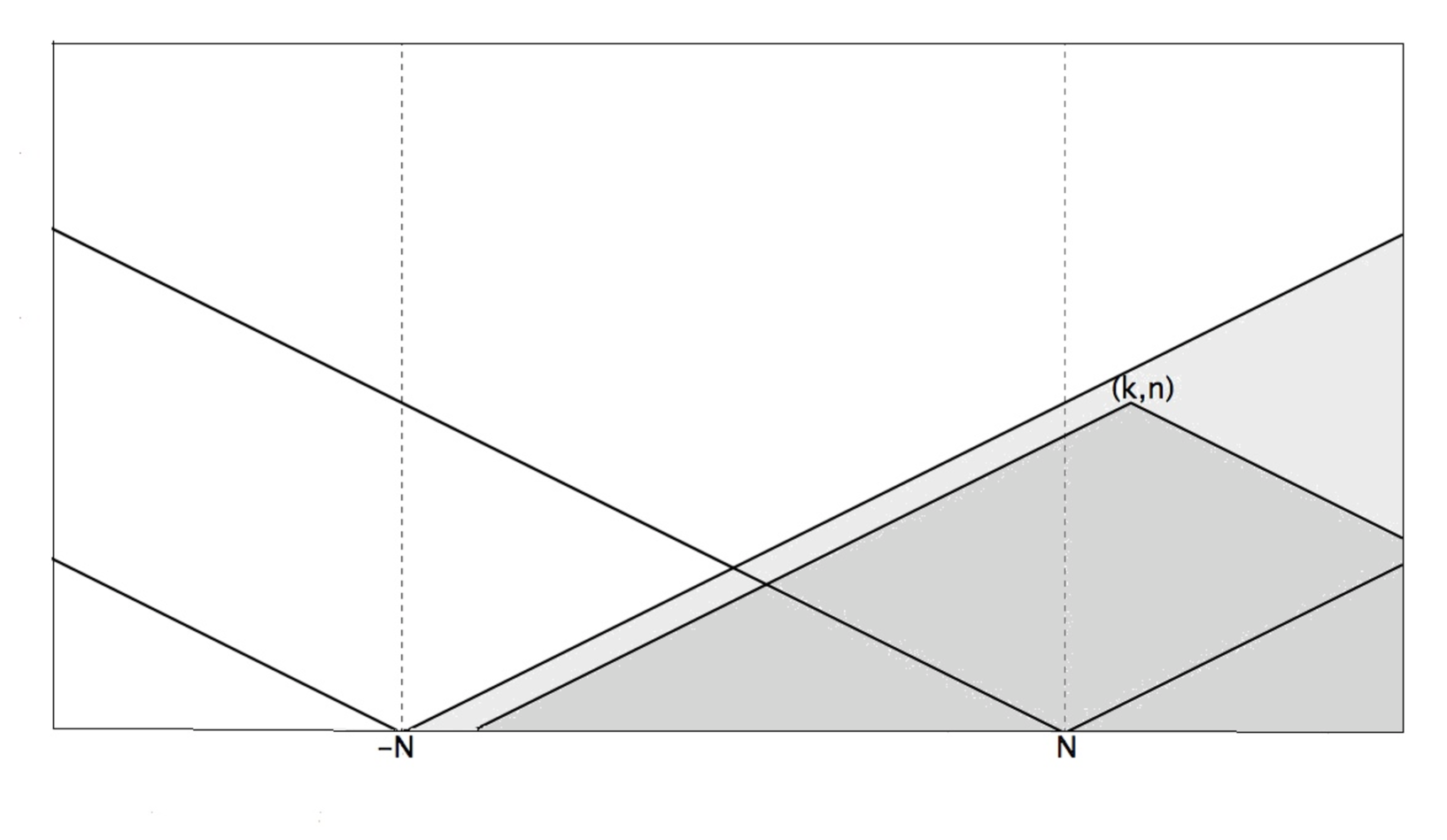
Figure 1: The shaded region represents the set $R$ in which $z^{+}_{h,m}=z^{-}_{h,m}$. The darker region is its intersection with a domain of dependence $C_{\mathbf{k,n}}$, when $k>2n-N$

The main issue in the proof of Theorem 1.2 consists in identifying the region in the plane $(k,n)$ in which $z_{k,n}^{+}=z_{k,n}^{-}$, this is set out by the following Lemma:

Lemma 2.3.

Let $R$ be the region below the line $k=2n-N$, that is

$$R=\{(k,n)\in\mathbb{Z}\times\mathbb{N}:\;k>2n-N\}.$$

Then we have $z_{k,n}^{+}=z_{k,n}^{-}$, for every $(k,n)\in R$, and consequently $\Lambda_{n}^{+}=\Lambda_{n}^{-}$ for $n\leq N-1$.

Proof.

Let us set

$$R_{n}=\{(k,j)\in R:\quad j\leq n\}.$$

We prove the assertion by induction on $n$. We have $z^{+}_{k,j}=z^{-}_{k,j}$ for $(k,j)\in R_{0}$, since the only non vanishing term is $z^{\pm}_{N,0}=1$. Assume that $z^{+}_{k,j}=z^{-}_{k,j}$ for every $(k,j)\in R_{n-1}$. Since the domain of dependence of $z^{\pm}_{k,n}$, with $(k,n)\in R_{n}$ is contained in $R_{n-1}$, we get $z^{+}_{k,j}=z^{-}_{k,j}$ for every $(k,j)\in R_{n}$.

We observe that the domain of dependence $C_{\mathbf{N,n}}$ of $\Lambda_{n}^{\pm}$ is contained in $R$ if $n\leq N-1$, thus the rest of the assertion follows by formula 2.11 and Lemma 2.2.

∎

Remark 2.4.

Let $G(t,q)$ be a function as in the assumptions of Theorem 1.2. If, for some $K>1$, we have $G_{i}\equiv 0$, for $i=1,\dots,K-1$, then, in addition to (A), we have

$$L_{N}(q)=O(q^{K}),\quad N\leq K.$$

In fact, from formula 2.11 we have immediately that $\Lambda_{i}^{\pm}=0$ for $i<K$, for $i=1,\dots,K-1$.

Remark 2.5.

Let $m\geq 1$ be a fixed integer, and let us weaken the assumption on the $\pi$-periodic coefficients $G_{n}$ by requiring that they are polynomials of degree at most $2n$, for $n\leq m$ (instead of $n\in\mathbb{N}$). Then Lemmas 1, and 2 hold true up to the level $m$. This means that in Lemma 1, the domain of dependence of $z_{k,n}^{\pm}$ is still $C_{\mathbf{k,n}}$, provided $n\leq m$, while in Lemma 2, we have $z_{k,n}^{+}=z_{k,n}^{-}$, for every $(k,n)\in R$, with $n\leq m$. It follows that in Theorem 1.2, we still have $L_{N}(q)=O(q^{N})$ for the first $m$ instability tongues.

For future reference, we report here the computation of the two first coefficients $\Lambda_{1}^{\pm}$ and $\Lambda_{2}^{\pm}$ of $\lambda_{N}^{\pm}(q)$ in 2.2. By using 2.8, 2.9 and 2.11, we get the following expressions,

$$\Lambda^{\pm}_{1}(1)=-G_{0,1}\mp\frac{1}{2}G_{1,1},\qquad\Lambda^{\pm}_{1}(N)=-G_{0,1},\qquad N=0,\quad N\geq 2.$$ (2.14)

$$\Lambda^{\pm}_{2}(1) = -G_{0,2}-\frac{1}{32}G_{1,1}^{2}\mp\frac{1}{2}G_{1,2},$$ (2.15)

$$\Lambda^{\pm}_{2}(2) = -G_{0,2}+\frac{1}{24}G_{1,1}^{2}\pm\left(-\frac{1}{2}G_{2,2}+\frac{1}{16}G_{1,1}^{2}\right),$$ (2.16)

$$\Lambda^{\pm}_{2}(N) = -G_{0,2}+\frac{1}{8(N^{2}-1)}G_{1,1}^{2},\qquad N=0,\quad N\geq 3.$$ (2.17)

2.2 Proof of Theorem 1.2: Inverse problem

Here we consider the Hill equation 1.4 under the general assumption that $G$ is an even $\pi$ periodic function satisfying 2.1 without restrictions on the degree of $G_{n}$, and we prove the only if part of Theorem 1.2.

We remark that formula 2.11 for the coefficients in the expansion of the eigenvalues $\lambda^{\pm}_{N}(q)$ is now replaced by the the following summation

$$\Lambda_{n}^{\pm}=-\frac{1}{2}\sum_{s=1}^{n}\sum_{i=0}^{\infty}G_{i,s}\left(z_{N-2i,n-s}^{\pm}+z_{N+2i,n-s}^{\pm}\right).$$ (2.18)

First of all, let us prove that under assumption (A), $G_{1}$ is a polynomial of degree at most $2$. Let $N\geq 1$ be an arbitrary eigenvalue number, and let us apply formula 2.18 for $n=1$. We have

$$\Lambda_{1}^{\pm}=-\frac{1}{2}\sum_{i=0}^{\infty}G_{i,1}\left(z_{N-2i,0}^{\pm}+z_{N+2i,0}^{\pm}\right).$$

Since $z_{k,0}^{\pm}=\delta_{k,N}\pm\delta_{k,-N}$, we get

$$\Lambda_{1}^{\pm}=-G_{0,1}\mp\frac{1}{2}G_{N,1},$$

thus $\Lambda_{1}^{+}-\Lambda_{1}^{-}=-G_{N,1}$. We infer that $L_{N}(q)=-G_{N,1}q+O(q^{2})$ for every $N\geq 1$. Owing to the assumption (A), we conclude that $G_{N,1}=0$ for $N>1$, which proves the assertion.

Now let us consider an integer $m\geq 2$, and assume that

$$G_{n}(t)=\sum_{k=0}^{n}G_{k,n}\cos(2kt),\quad\text{ for every }n\leq m-1,$$ (2.19)

that is $G_{n}$ is a polynomial of degree at most $2n$ for $n\leq m-1$. We shall show that 2.19 leads to $L_{N}=-G_{N,m}q^{m}+O(q^{m+1})$, for every $N>m$. Thanks to (A) we conclude that $G_{N,m}=0$, for every $N>m$, which means that $G_{m}$ is a polynomial of degree at most $2m$. Thus the assertion will follow by induction on $m$.

Let us consider the $N$-th eigenvalue branch $\lambda^{\pm}_{N}$, with $N>m$. Under assumption 2.19, Lemma 2 and Lemma 3 hold true for all levels $n\leq m-1$ (see Remark 2.5), in particular $\Lambda_{n}^{+}=\Lambda_{n}^{-}$ for $n\leq m-1$. Let us apply 2.18 for $n=m$. We have

$$\Lambda_{m}^{\pm}=-\frac{1}{2}\sum_{s=1}^{m-1}\sum_{i=0}^{s}G_{i,s}\left(z_{N-2i,m-s}^{\pm}+z_{N+2i,m-s}^{\pm}\right)-\frac{1}{2}\sum_{i=0}^{\infty}G_{i,m}\left(z_{N-2i,0}^{\pm}+z_{N+2i,0}^{\pm}\right)$$ (2.20)

The first term on the right-hand side of 2.20 does not depend on the determinations $\pm$, since all the indices $(N\pm 2i,m-s)$ are in the region $R$, up to the level $m$; let $A$ be its value. Thus, by the initial conditions at level $n=0$, we get

$$\Lambda_{m}^{\pm}=A-G_{0,m}\mp\frac{1}{2}G_{N,m}.$$

It follows that $L_{N}=-G_{N,m}q^{m}+O(q^{m+1})$, for every $N>m$. This concludes the proof of Theorem 1.2.

2.3 Existence of finitely many tongues

We point out that not only the instability tongues can be thinner than predicted by the general result, but can even disappear. We will show some examples of existence of finitely many tongues in Section 5.

The question of the existence of finitely many instability intervals (gaps) for the Hill equation,

$$z^{\prime\prime}(t)+(\beta+Q(t))z(t)=0$$

has been deeply investigated by many authors, and dates back to the work of Ince [24] on the impossibility of the coexistence for the Mathieu equation, see [29, ch. VII], and [13] for interesting extensions and a recent account of the subject. A detailed study of the coexistence problem for the related Ince equation is provided by [36].

Starting from the introduction of the Lax pairs formulation of the KdV hierarchy as a compatibility relation with the Hill operator, research on the multiplicity of eigenvalues has come to a remarkable and celebrated result, essentially thanks to the work of Lax [27] and Novikov [34] around 1975 (see also [21]): at most $n$ instability intervals fail to vanish if and only if $Q$ satisfies a differential equation of the form,

$$Q^{(2n)}+H(Q,Q^{\prime},\dots,Q^{(2n-2)})=0,$$ (2.21)

where $H$ is a polynomial of maximal degree $n+2$. It turns out that equation 2.21 is equivalent to a linear combination of the first $n$-order stationary KdV equations. We refer to [20] for an extensive bibliography, and a clear presentation of the modern theory.

In the starting case $n=1$, there exists exactly one finite instability interval if and only if $Q(t)$ satisfies the equation $\,Q^{\prime\prime}+AQ+B+3Q^{2}=0\,$ for suitable real constants $A$, $B$ (the first proof of the necessity of this condition is due to Hochstadt [23]).

For $n>1$, in the rest of the paper we will refer to the following classical result of Ince [25, 16] [29, ch. VII], on a particular class of elliptic coefficient of the Hill equation offering the simplest example for which all but $n$ finite instability intervals disappear. Here we state the theorem in a favorable form for our purposes, see Appendix B for a brief discussion.

Theorem 2.6 (The Ince theorem).

Let $Q$ be a non constant periodic solution of the differential equation,

$$Q^{\prime\prime}+AQ+B+3Q^{2}=0$$ (2.22)

where $A$, $B$ are real numbers such that $A^{2}-12B>0$. Then, for every positive integer $n$, the Hill equation,

$$z^{\prime\prime}(t)+\left(\beta+\frac{n(n+1)}{2}\,Q(t)\right)z(t)=0$$

has exactly $n+1$ instability intervals, including the unbounded one.

In Section 5 we will provide some examples of coupled equations 1.1–1.2 where equation 1.1 can be written in the form,

$$z^{\prime\prime}(t)+\left(\beta+\gamma\,Q(t,q)\right)z(t)=0$$

with $Q(t,q)$ satisfying 2.22 for every $q$. As a consequence, if $\displaystyle{\gamma=\frac{n(n+1)}{2}}$, only a finite number of tongues fail to vanish.

3 Proof of Theorem 1.1

In this section we prove Theorem 1.1. In the first part we provide the asymptotic development of the periodic solutions of equation 1.2 by removing secular terms as in the classical Poincaré–Lindstedt method. In the second part we insert the development in the Hill equation 1.1, and after an adequate normalization of the coefficients, we show that the assumptions of Theorem 1.2 are satisfied.

3.1 Expansion of the solution of equation 1.2

Let $u(t,q)$ be the solution to the initial-values problem 1.2. According to our assumptions on the function $f$, we write the Taylor series of $f$ in a neighborhood of $0$:

$$f(x)=\sum_{k=2}^{\infty}\alpha_{k}x^{k},\qquad|x|<r_{0}.$$

Let $r_{1}$ be the least modulus of the singular points of the equation 1.2, that is $r_{1}=\min\{|x|:\,4x+f(x)=0\}$, $r_{0}=+\infty$ in case the set is empty. The parameter $q$ will be subject to several restrictions, the first one being $|q|<\min\{r_{0},r_{1}\}$ so that the solution of 1.2 are periodic and depend analytically on $q$. From now on we simply assume that the parameter $q$ is small enough so that our power series converge.

Let us denote by $T(q)$ the period of $u(t,q)$ and by $\omega(q)=\pi/T(q)$ its angular frequency. Both depend analytically on $q$ in some (in general) smaller neighborhood of $0$, thus we can write the following power series expansion ($\Omega_{0}=1$),

$$\Omega(q)=\omega(q)^{2}=\sum_{n=0}^{\infty}q^{n}\Omega_{n}.$$ (3.1)

If we rescale time in 1.2 by setting $\tau=\omega(q)t$, and the solution $u(t,q)=qU(\tau,q)$, so that $U(\tau+\pi;q)=U(\tau,q)$, the problem 1.2 reads as follows,

$$\Omega(q)U^{\prime\prime}(\tau)+4U(\tau)+\sum_{n=1}^{\infty}\alpha_{n+1}q^{n}U(\tau)^{n+1}=0,\qquad U(0)=1,\quad U^{\prime}(0)=0.$$ (3.2)

By the Poincaré expansion theorem (see [35, Th. 9.2]), $U(\tau,q)$ can be expressed, on the fixed time interval $[0,\pi]$ (thus on $\mathbb{R}$), as a convergent power series with respect to $q$ in a neighborhood of $0$, uniformly with respect to $\tau$:

$$u(t,q)=qU(\tau,q)=\sum_{n=1}^{\infty}q^{n}u_{n}(\tau).$$ (3.3)

The coefficients $u_{n}$ in the expansion 3.3 are periodic and, by the initial conditions in 3.2, we obtain that

$$u_{n}(\tau+\pi)=u_{n}(\tau),\quad u_{1}(\tau)=\cos(2\tau),\quad u_{n}(0)=u^{\prime}_{n}(0)=0,\quad n\geq 2.$$ (3.4)

If we plug the expansion 3.3 into the problem 3.2 we get, in addition to conditions 3.4, the sequence of recurrent differential equations,

$$u_{1}^{\prime\prime}+4u_{1}=0,$$ (3.5)

$$u_{2}^{\prime\prime}+4u_{2}=-\Omega_{1}u_{1}^{\prime\prime}-\alpha_{2}u_{1}^{2},$$ (3.6)

$$u_{3}^{\prime\prime}+4u_{3}=-\Omega_{2}u_{1}^{\prime\prime}-\Omega_{1}u_{2}^{\prime\prime}-2\alpha_{2}u_{1}u_{2}-\alpha_{3}u_{1}^{3},$$ (3.7)

and in general, for $n>3$,

$$u_{n}^{\prime\prime}+4u_{n}=F_{n}(\tau)$$ (3.8)

where

$$F_{n}(\tau)=-\sum_{k=1}^{n-1}\Omega_{k}u_{n-k}^{\prime\prime}-\sum_{k=2}^{n}\alpha_{k}\sum_{i_{1}+\dots+i_{k}=n}u_{i_{1}}\cdots u_{i_{k}}$$

Periodic solutions of the $n$-th recurrent equation are possible if secular terms are removed from the right-hand side of the equation, so that the coefficient of the resonant term in $F_{n}(\tau)$ vanishes. This means that we have to impose that $\int_{0}^{\pi}F_{n}(\tau)\cos(2\tau)\,{\rm d}\tau=0$, which is the first step to obtain the asymptotic expansions of $\omega(q)$, and subsequently of $u(t)$, by the Poincaré–Lindstedt method (see [35, ch. 10]).

By a simple inductive argument, we can show the following property of the coefficients $u_{n}$:

Proposition 3.1.

The coefficients $u_{n}(\tau)$, $n\geq 1$ in the power series 3.3 are even $\pi$-periodic trigonometrical polynomials of degree $2n$.

Proof.

We prove the assertion by induction on $n\in\mathbb{N}$. It is obviously true for $n=1$, and let us assume it is true for $1\leq j\leq n-1$ ($n\geq 2$). By a simple computation, it follows that the multilinear terms in $F_{n}(\tau)$ of the $n$-th recursive differential equation, that is

$$\sum_{i_{1}+\dots+i_{k}=n}u_{i_{1}}u_{i_{2}}\cdots u_{i_{k}},$$

and the term $\sum_{k=1}^{n-1}\Omega_{k}u_{n-k}^{\prime\prime}$, are even $\pi$-periodic polynomials of degree $\leq 2n$. Thus, once the resonance has been removed, the source term $F_{n}$ in the $n$-th equation has the following expression,

$$F_{n}(\tau)=\sum_{k=0,k\neq 1}^{n}c_{k}\cos(2k\tau).$$

Therefore, recalling that $u_{n}(0)=u_{n}^{\prime}(0)=0$, the solution of the $n$-th problem, is given by

$$u_{n}(\tau)=\sum_{k=0,k\neq 1}^{n}\frac{c_{k}}{4-4k^{2}}\cos(2k\tau)-\sum_{k=0,k\neq 1}^{n}\frac{c_{k}}{4-4k^{2}}\cos(2\tau),$$

which proves the assertion. ∎

3.2 Hill Equation

Here we turn our attention to the periodic eigenvalues problem for the Hill equation 1.1. We need to rewrite the equation in the form 1.4: we rescale the time variable, $\tau=\omega(q)t$, set $z(t)=Z(\omega(q)t)$. Then, by introducing the new coefficients,

$$\lambda(q)=\beta(q)/\Omega(q),\qquad G(\tau,q)=g(qU(\tau,q))/\Omega(q),$$ (3.9)

we get rid of the $\Omega(q)$ factor by absorbing it in a modified eigenvalues problem, so that we obtain a Hill equation with fixed period $\pi$:

$$Z^{\prime\prime}(\tau)+\left(\lambda(q)+G(\tau,q)\right)Z(\tau)=0.$$ (3.10)

Lemma 3.2.

Let $g$ be a real analytical function in a neighborhood of $0$, $g(0)=0$, and let $U(\tau,q)$ be the solution of problem 3.2. Then the following expansion holds true in a neighborhood of the origin, uniformly with respect to $\tau$,

$$G(\tau,q)=\sum_{n=1}^{\infty}q^{n}G_{n}(\tau),\quad\tau\in\mathbb{R},$$ (3.11)

where $G_{n}(\tau)$ is an even $\pi$-periodic trigonometrical polynomial of degree $2n$ as in formula 1.6.

Proof.

From our assumptions we may write, for $q$ and $x$ sufficiently small,

$$g(x)=\sum_{k=1}^{\infty}\gamma_{k}x^{k},\qquad\frac{1}{\Omega(q)}=\sum_{n=0}^{\infty}\kappa_{n}q^{n}.$$ (3.12)

By composition of analytical functions, we obtain

$$g(qU(\tau,q))=\sum_{n=1}^{\infty}q^{n}g_{n}(\tau),$$

where the coefficients $g_{n}(\tau)$ are given by the following expressions,

$$g_{n}(\tau)=\sum_{k=1}^{n}\gamma_{k}\sum_{h_{1}+\dots+h_{k}=n}u_{h_{1}}\cdots u_{h_{k}}.$$ (3.13)

From Proposition 3.1, and by a simple computation, we get that $g_{n}(\tau)$ is an even $\pi$-periodic trigonometrical polynomial whose degree does not exceed $2n$. The assertion follows since $G_{n}$, owing to 3.9, 3.12 is a linear combination of $g_{j}$, $j\leq n$, that is

$$G_{n}(\tau)=\sum_{j=0}^{n}g_{j}(\tau)\kappa_{n-j}.$$ (3.14)

∎

3.3 Conclusion of the proof of Theorem 1.1

Let us write the power series expansion of $\beta^{\pm}_{N}(q)$,

$$\beta^{\pm}_{N}(q)=N^{2}+\sum_{n=1}^{\infty}B^{\pm}_{n}(N)q^{n},$$ (3.15)

where, from 3.9, the coefficients are given by

$$B_{n}^{\pm}(N)=\sum_{j=0}^{n}\Lambda_{j}^{\pm}(N)\,\Omega_{n-j}.$$ (3.16)

Owing to Lemma 2.3, the assumptions of Theorem 1.2 are satisfied by the equation 3.10. It follows that for any eigenvalue number $N$, the coefficients in the expansion of $\lambda_{N}^{\pm}$ satisfy $\Lambda^{+}_{n}(N)=\Lambda^{-}_{n}(N)$, for $n<N$, thus $B_{n}^{+}(N)=B_{n}^{-}(N)$, for $n<N$ which proves the assertion. In particular for the leading term in the expansion (A), we have

$$C_{N}=B_{N}^{+}(N)-B_{N}^{-}(N)=\Lambda_{N}^{+}(N)-\Lambda_{N}^{-}(N).$$

$\square$

3.4 Additional results

In certain cases it is possible to provide a more precise asymptotic expansion of $L_{N}(q)$, as it is shown in the following Proposition.

Proposition 3.3.

Let $K\geq 1$ be the first non-vanishing power in the expansion 3.12 of $g(x)$, that is $g(x)=\gamma_{K}x^{K}+O(x^{K+1})$, $\gamma_{K}\neq 0$. Then, for every $1\leq N\leq K$, we have

$$L_{N}(q)=C_{K,N}\,q^{K}+O(q^{K+1}),$$ (3.17)

In addition, $C_{K,N}\neq 0$ when $N$ and $K$ have the same parity, whereas $C_{K,N}=0$ when $K-N$ is odd.

Proof.

If $K>1$, from formula 3.13, we get $g_{n}(\tau)\equiv G_{n}(\tau)\equiv 0$, for $n<K$. Then, owing to Remark 2.4, we have that $\Lambda_{n}(N)=0$ for $n<K$. From formula 3.16, it follows that $B_{n}^{\pm}(N)=N^{2}\Omega_{n}$, for $n<K$. This proves that $L_{N}(q)=O(q^{K})$ for $0<n<K$.

Let $K\geq 1$. By using condition 2.8, and formula 2.11, we can compute the coefficient $\Lambda_{K}^{\pm}(N)$ for $N\leq K$. This reduces to

$$\Lambda_{K}^{\pm}(N)=-\frac{1}{2}\sum_{i=0}^{K}G_{i,K}\left(z_{N-2i,0}^{\pm}+z_{N+2i,0}^{\pm}\right)=-G_{0,K}\mp\frac{1}{2}G_{N,K}.$$ (3.18)

Then we have $C_{K,N}=\Lambda_{K}^{+}(N)-\Lambda_{K}^{-}(N)=-G_{N,K}$. From formulas 3.13 and 3.14, we get that

$$G_{K}(\tau)=g_{K}(\tau)=\gamma_{K}(u_{1}(\tau))^{K}=\gamma_{K}(\cos(2\tau))^{K}.$$ (3.19)

Since $G_{N,K}$ is the $2N$-th Fourier coefficient of $G_{K}(\tau)$, we obtain

$$G_{N,K}=\frac{2\gamma_{K}}{\pi}\int_{-\pi/2}^{\pi/2}{\cos(2\tau)^{K}\,\cos(2N\tau){\rm d}\tau}.$$ (3.20)

This integral does not vanish if and only if $K$ and $N$ have the same parity, as it follows by the following formula

$$2^{K-1}\cos(2\tau)^{K}=\cos(2K\tau)+K\cos(2(K-2)\tau)+\binom{K}{2}\cos(2(K-4)\tau)+\cdots\,.$$

In particular, for $K-N=2m$, we get the expression $\displaystyle C_{K,N}=-\frac{\gamma_{K}}{2^{K-1}}\binom{K}{m}$.

∎

For example, if $g(x)=\gamma_{4}x^{4}+O(x^{5})$, the second and fourth tongues have order of tangency equal to $4$, in particular they do not collapse to a single line, while the first and third tongues have a contact of order at least $5$.

As an immediate consequence, if $g^{\prime}(0)=\gamma_{1}\neq 0$, the first instability tongue never reduces to a single curve:

Corollary 3.4.

For every function $f$ satisfying the assumptions of Theorem 1.1, if $g^{\prime}(0)\neq 0$, then the first instability tongue of equation 1.1 cannot collapse to a single line, that is $L_{1}(q)\neq 0$.

Remark 3.5.

As we mentioned in the introduction, in our discussion of the instability tongues, we assumed that equation 1.1 has the same period $T(q)$ as $u(t)$. As a matter of fact, the period of $g(u(t))$ may be a fraction of $T(q)$; this occurs for instance when $f$ and $g$ are odd and even functions respectively, and the period of $g(u(t))$ is half the period of $u(t)$. In this case, the potential function $2u^{2}+\int_{0}^{u}f(x)\,dx$ of equation 1.2 is an even function, thus $u(t+T(q)/2)=-u(t)$ which yields $g(u(t+T(q)/2))=g(u(t))$.

It follows that the real eigenvalues of the problem branch out only for even $N$, or in other words $L_{N}(q)\equiv 0$ for odd $N$. The asymptotic estimate (A) of Theorem 1 is of course satisfied with $C_{N}=0$ for odd $N$.

4 Shape of the instability tongues

The purpose of this section is to characterize the form of instability tongues related to the system 1.2–1.1 for small $q$. Applications to some significant cases related to the theory of suspension bridges are provided in Section 5.

From the geometrical point of view, we observe that the instability tongues starting from $\beta^{\pm}_{N}(0)=N^{2}$ may be either “trumpet shaped” if one of the curves $\beta=\beta^{\pm}_{N}(q)$ is decreasing and the other increasing, or “horn shaped” if are both increasing or both decreasing. For instance, in the case of the Mathieu equation (see also the following Proposition 4.1) it is well-known that the first two tongues are trumpet shaped while the others are horn shaped for small values of $q$.

The question is relevant for stability analysis at small energies when we consider the parameter $\beta$ in 1.1 as fixed. In case of a trumpet shaped tongue, the line $\beta=N^{2}$ falls into the instability region (at least for $q$ small), and the intersection of the tongue with a straight line $\beta=const$ close to $N^{2}$, after a small interval of stability, intercepts a long interval of instability. Viceversa, for a horn shaped tongue, the intersection with a straight line $\beta=const$ close to $N^{2}$ is at most a very small segment.

In the following proposition, $\alpha$ and $\gamma$ coefficients refer to the power series expansion of $f$ and $g$ respectively.

Proposition 4.1.

The asymptotic behavior of the instability tongues, up to second order in $q$ is the following:

The first tongue is always trumpet shaped if $\gamma_{1}\neq 0$. It has an approximate length $L_{1}(q)=-\gamma_{1}(q+\frac{1}{12}\alpha_{2}q^{2})+o(q^{2})$, as $q\to 0$.

The second tongue has an approximate length $L_{2}(q)=(\frac{1}{8}\gamma_{1}^{2}-\frac{1}{24}\gamma_{1}\alpha_{2}-\frac{1}{2}\gamma_{2})q^{2}+o(q^{2})$, as $q\to 0$. It may be either trumpet or horn shaped, depending on the parameters.

As for the next tongues, they are generically horn shaped, with the exception of very particular values of the parameters for which $B^{\pm}_{j}(N)=0$, $j<N$.

Although it does not geometrically correspond to a tongue, we may consider also the case $N=0$, when the (even) periodic eigenvalue $\beta=\beta^{+}_{0}(q)$ forms the right boundary of an unbounded region of instability. In this case we have

$$\beta_{0}^{+}(q)=\left[\frac{\gamma_{1}}{8}(\alpha_{2}-\gamma_{1})-\frac{\gamma_{2}}{2}\right]q^{2}+O(q^{3}),$$

thus the line $\beta=0$ lies or not in the instability region, at least for small values of $q$, depending on the sign of $B_{2}^{+}(0)=\gamma_{1}(\alpha_{2}-\gamma_{1})/8-\gamma_{2}/2$.

Figure 2: Instability tongues of Mathieu equation. The first two tongues are trumpet shaped, the others horn shaped

The proof of Proposition 4.1 is a consequence of the following two lemmas. Let us start with direct computation of the first coefficients of $\Omega$, and $U$ in 3.1, 3.2, in the case when $\alpha_{2}$, $\alpha_{3}$ are not both vanishing, which is the most interesting for applications.

Lemma 4.2.

From the first recurrent equations 3.5, 3.6, 3.7, we have the following expressions,

$$\Omega_{1}=0,\qquad u_{2}(\tau)=\alpha_{2}\left(-\frac{1}{8}+\frac{1}{12}\cos 2\tau+\frac{1}{24}\cos(4\tau)\right),$$ (4.1)

$$\Omega_{2}=-\frac{5}{96}\alpha_{2}^{2}+\frac{3}{16}\alpha_{3}.$$ (4.2)

Proof.

Since $u_{1}(\tau)=\cos 2\tau$, equation 3.6 reads as

$$u_{2}^{\prime\prime}+4u_{2}^{\prime\prime}=4\Omega_{1}\cos 2\tau-\frac{\alpha_{2}}{2}-\frac{\alpha_{2}}{2}\cos 4\tau,$$

thus elimination of the resonant term, and an easy check yields formula 4.1. Then equation 3.7, after substitution, becomes

$$u_{3}^{\prime\prime}+4u_{3}=\left(4\Omega_{2}+\frac{5}{24}\alpha_{2}^{2}-\frac{3}{4}\alpha_{3}\right)\cos(2\tau)-\frac{\alpha_{2}^{2}}{12}-\frac{\alpha_{2}^{2}}{12}\cos(4\tau)-\left(\frac{\alpha_{3}}{4}+\frac{\alpha_{2}^{2}}{24}\right)\cos(6\tau),$$

and if one removes the resonant term, will get formula 4.2. ∎

Next from equation 3.10, we compute the approximation of the tongues, up to second power in $q$. This approximation is significant if $\gamma_{1}$, $\gamma_{2}$ are not both vanishing.

Lemma 4.3.

The first two coefficients in the expansion 3.15 have the following expressions,

$$B^{\pm}_{1}(1) = \mp\frac{1}{2}\,\gamma_{1},\qquad B^{\pm}_{1}(N)\;=\;0,\quad\text{ for }N>1\;\text{ or }N=0,$$

$$B^{\pm}_{2}(1) = \Omega_{2}+\frac{1}{8}\gamma_{1}\alpha_{2}-\frac{1}{2}\gamma_{2}-\frac{1}{32}\gamma_{1}^{2}\mp\frac{1}{24}\gamma_{1}\alpha_{2},$$

$$B^{\pm}_{2}(2) = 4\Omega_{2}+\frac{1}{8}\gamma_{1}\alpha_{2}-\frac{1}{2}\gamma_{2}+\frac{1}{24}\gamma_{1}^{2}\mp\frac{1}{48}\left(\gamma_{1}\alpha_{2}-3\gamma_{1}^{2}+12\gamma_{2}\right),$$

$$B^{\pm}_{2}(N) = N^{2}\Omega_{2}+\frac{1}{8}\gamma_{1}\alpha_{2}-\frac{1}{2}\gamma_{2}+\frac{1}{8(N^{2}-1)}\gamma_{1}^{2},\quad\text{ for }N>2\text{ or }N=0.$$

Proof.

We go back to 3.10 and observe that the first terms of $G(\tau,q)$ in 3.14 are given by

$$G_{1}(\tau)=g_{1}(\tau)=\gamma_{1}u_{1}(\tau),\quad G_{2}(\tau)=g_{2}(\tau)=\gamma_{1}u_{2}(\tau)+\gamma_{2}u_{1}^{2}(\tau)$$ (4.3)

being $\kappa_{0}=1$, $\kappa_{1}=0$ in 3.14, and $g_{1}(\tau)$, $g_{2}(\tau)$ as in 3.13.

Then we insert $u_{1}(\tau)=\cos(2\tau)$ and $u_{2}(\tau)$ as in in 4.3 of Proposition 4.2, and obtain the following coefficients

$$G_{0,1} = 0,\quad G_{1,1}=\gamma_{1},$$

$$G_{0,2} = -\frac{1}{8}\gamma_{1}\alpha_{2}+\frac{1}{2}\gamma_{2},\quad G_{1,2}=\frac{1}{12}\gamma_{1}\alpha_{2},\quad G_{2,2}=\frac{1}{24}\gamma_{1}\alpha_{2}+\frac{1}{2}\gamma_{2}.$$

Finally, since $\Lambda_{0}^{\pm}(N)=N^{2}$, $\Omega_{0}=1$, $\Omega_{1}=0$, we have in 3.16

$$B_{1}^{\pm}(N)=\Lambda_{1}^{\pm}(N),\quad B_{2}^{\pm}(N)=\Lambda_{2}^{\pm}(N)+N^{2}\Omega_{2},$$

and by simple substitutions in 2.15, 2.16, 2.17, we have the assertion. ∎

One may wonder if there exists some universal upper bound for the number of trumpet shaped tongues. In the following proposition we provide a negative answer, by showing that, with a suitable choice of the functions $f$, $g$, the number of trumpet shaped tongues can be arbitrarily large.

Proposition 4.4.

Let $K\geq 1$ be an odd integer, and let $\alpha_{K+1}$, $\gamma_{K}$ be the first non-vanishing coefficients in the power series expansion of $f$ and $g$ respectively. Then the tongues corresponding to odd $N$, for $1\leq N\leq K$, are trumpet shaped, and their order of tangency at $q=0$ is exactly $K$.

Proof.

For $K=1$ the statement follows from Proposition 4.1. Let us consider $K\geq 3$. We claim that in the power series 3.1 of $\Omega(q)$, we have $\Omega_{j}=0$ for $1\leq j\leq K$.

Since $\alpha_{j}=0$, and for $2\leq j\leq K$, by a simple inductive argument applied to the recursive equations 3.8, we have that $u_{j}=0$ for $1\leq j\leq K$, and $\Omega_{j}=0$ for $1\leq j\leq K-1$.

It remains to prove that $\Omega_{K}=0$. The equation for $u_{K+1}$ reduces to

$$u_{K+1}^{\prime\prime}+4u_{K+1}=4\Omega_{K}u_{1}-\alpha_{K+1}u_{1}^{K+1},$$

and the coefficient $\Omega_{K}$ is computed by removing the resonance term $\cos(2t)$ in the right-hand side term. Therefore we get

$$4\Omega_{K}=\alpha_{K+1}\,\frac{2}{\pi}\int_{-\pi/2}^{\pi/2}u_{1}^{K+1}(\tau)\cos(2\tau)\,{\rm d}\tau=\alpha_{K+1}\,\frac{2}{\pi}\int_{-\pi/2}^{\pi/2}\cos^{K+2}(2\tau)\,{\rm d}\tau.$$

The claim is proved, since this integral vanishes when $K$ is odd.

Now, from formula 3.16, it follows that $B^{\pm}_{j}(N)=\Lambda^{\pm}_{j}(N)$, for $1\leq j\leq K$, $N\leq K$. In addition, since $G(\tau,q)=g(qU(\tau,q))/\Omega(q)=\gamma_{K}q^{K}\cos(2\tau)^{K}+O(q^{K+1})$, owing to Remark 2.4, we get

$$B^{\pm}_{j}(N)=\Lambda^{\pm}_{j}(N)=0\qquad(1\leq j<K).$$

On the other hand, from formula 3.18 in Proposition 3.3, we have

$$B^{\pm}_{K}(N)=\Lambda^{\pm}_{K}(N)=-G_{0,K}\mp\frac{1}{2}G_{N,K},$$

where $G_{N,K}$, as computed by formula 3.19 is not zero, if $N$ has the same parity of $K$. Finally, for odd $K$, we get

$$G_{0,K}=\frac{\gamma_{K}}{\pi}\int_{-\pi/2}^{\pi/2}{\cos^{K}(2\tau)\,{\rm d}\tau}=0.$$

The conclusion is that $B_{j}^{\pm}(N)=0$, for $1\leq j\leq K-1$, and $B^{+}_{K}(N)=-B^{-}_{K}(N)\neq 0$, which proves the assertion. ∎

Remark 4.5.

In many applications the function $g$ is proportional to the derivative of $f$, i.e. $g(x)=\tilde{\gamma}f^{\prime}(x)$. In these cases we obviously have $\gamma_{n}=0\,\Longleftrightarrow\,\alpha_{n+1}=0$

Under this assumption, Proposition 4.4 yields examples of trumpet shaped tongues with the same order of tangency.

5 Applications to suspension bridges and examples

In this section we come back to the problem that gave rise to our investigations, and we illustrate a few results related to problem (II) (see introduction).

An important issue in the mathematical modeling of suspension bridges is the phenomenon of energy transfer from flexural to torsional modes of vibration along the deck of the bridge. According to a recent field of research [3, 8, 19, 17, 10] internal nonlinear resonances giving rise to the onset of instability may occur even when the aeroelastic coupling is disregarded. In particular, in the fish-bone bridge model ([19, ch. 3], or [30]), the non-linear coupling between flexural and torsional oscillation of the bridge is described by the function $\mathcal{F}(x)$, which represents in the PDEs system the restoring action of the pre-stressed hangers. A first expression of such $\mathcal{F}$ was proposed in [32, 33]:

$$\mathcal{F}(x)={\rm k}\left[(x+x_{0})^{+}-x_{0}\right].$$

Under this assumption, the PDEs system acts as a linear uncoupled system for sufficiently low energy.

Anyway, other expression of $\mathcal{F}$ have been proposed in [30, 7, 31] and some of these are nonlinear and analytical function in a neighborhood of the origin. In that case some instability zone for low energy may be expected.

The second step in the cited papers is to reduce the PDE-system to an ODEs one, through a Galerkin projection. If, for sake of simplicity, our aim is to study the interaction between a single torsional mode and a single flexural one (the first ones, for example), the instability at a given energy level of a pure flexural solution is equivalent to the instability of an Hill equation like 1.1. More precisely, we are led to study a system of two coupled equations (the linearized system around the pure flexural solution). Such ODEs system can be written in the form 1.1–1.2 where the function $f(x)$ in 1.2 is strictly related to the function $\mathcal{F}$ in the PDEs model and the functions $g$ and $f$ in 1.1–1.2 satisfy $g(x)=\tilde{\gamma}f^{\prime}(x)$, $\tilde{\gamma}>0$, (see [8, 30]).

Our work proves that the thickness of the instability tongues gets thinner and thinner for growing $N$, then the most significant instability zones correspond to the first tongues; moreover, the parameter $\beta$ being constant in the applications, the shape of the tongues is also important, because entering deeply an instability zone is more destructive than being near to its border.

Now we present some simple examples of application of Proposition 4.1.

Example 1. Our first example is given by the following system,

$$u^{\prime\prime}(t,q)+4u(t,q)+\alpha u^{2}(t,q)=0,\qquad u(0;q)=q,\quad u^{\prime}(0;q)=0,$$

$$z^{\prime\prime}(t)+(\beta+2\tilde{\gamma}\alpha u(t,q))z(t)=0.$$

Owing to Propositions 4.2, we know that the first tongue is trumpet shaped and length $L_{1}(q)=-2\tilde{\gamma}\alpha q+O(q^{2})$. The second tongue is trumpet shaped if and only if

$$\tilde{\gamma}<-1,\quad\frac{1}{2}<\tilde{\gamma}<1,\quad\tilde{\gamma}>\frac{5}{2}.$$

We can also prove that coexistence may occur for special values of the parameters; precisely if $\tilde{\gamma}=\frac{n(n+1)}{12}$ ($n\in\mathbb{N}$) , then there exist only $n$ instability tongues, or equivalently there exist $2n+1$ simple eigenvalues.

In fact, if we set $\gamma=2\tilde{\gamma}\alpha$ for sake of simplicity, and plug $Q(t)=\gamma u(t)$ into 2.22, we get

$$u^{\prime\prime}+Au+B/\gamma+3\gamma u^{2}=0,$$

which is satisfied with the choice $A=4$, $B=0$, $\gamma=\alpha/3$. Thus the result follows by Theorem 2.6.

The following formula (see [37, Th. 5.3]) shows that the simple eigenvalues are the lowest ones:

$$C_{N}=\frac{(-1)^{N}\,\alpha^{N}}{8^{N-1}\,((N-1)!)^{2}}\prod_{k=0}^{N-1}\left(2\tilde{\gamma}-\frac{k(k+1)}{6}\right).$$

In addition $C_{N}\neq 0$ for every $N$, if $\tilde{\gamma}$ does not take one of the values $n(n+1)/12$.

Example 2. Our second example has been discussed for fixed values of the parameter $\tilde{\gamma}$ in [18] ($\tilde{\gamma}=1/3$), and [8] ($\tilde{\gamma}=3$). It is provided by the following coupled system,

$$u^{\prime\prime}(t,q)+4u(t,q)+\alpha u^{3}(t,q)=0,\qquad u(0;q)=q,\quad u^{\prime}(0;q)=0,$$

$$z^{\prime\prime}(t)+(\beta+3\tilde{\gamma}\alpha u^{2}(t,q))z(t)=0.$$

We observe that this second example falls within the conditions of Remark 3.5, so that the coefficient $g(u)$ has fundamental period $T(q)/2$. Thus the genuine instability tongues branch off from the $\beta$-axis at $\beta_{N}(0)=(2N)^{2}$, $N\in\mathbb{N}$.

The first tongue is trumpet shaped if and only if

$$\frac{1}{3}<\tilde{\gamma}<1.$$

Coexistence may occur for some values of the parameters; precisely if $\tilde{\gamma}=\frac{n(n+1)}{6}$, then there exist only $n$ instability tongues (in particular if $\tilde{\gamma}=\frac{1}{3}$, there is only the first one).

To prove this last assertion, let us set $\gamma=3\tilde{\gamma}\alpha$ and $Q(t)=\gamma u^{2}(t)$, and plug it into 2.22. We obtain

$$(u^{\prime})^{2}+uu^{\prime\prime}+\frac{A}{2}u^{2}+\frac{B}{2\gamma}+\frac{3}{2}\gamma u^{4}=0.$$ (5.1)

The first equation multiplied by $u^{\prime}$ yields the identity,

$$(u^{\prime})^{2}+4u^{2}+\frac{\alpha}{2}u^{4}=2E(q),$$

where $E(q)=4q^{2}+\alpha q^{4}/2$ is the energy of $u$. By replacing $(u^{\prime})^{2}$ in 5.1, we get

$$uu^{\prime\prime}+(\frac{A}{2}-4)u^{2}+(\frac{3}{2}\gamma-\frac{\alpha}{2})u^{4}+(2E-\frac{B}{2\gamma})=0.$$

Choosing $B=4\gamma E$ we get rid of the constant term. Finally by setting $A=16$, $\gamma=\alpha$, equation 2.22 is satisfied.

Example 3. In [31] we numerically studied the behavior of the ODEs system for some other functions. One of those was

$$\tilde{f}(x)=mx+m\sqrt{x^{2}+(h/m)^{2}}\,\,-h=mx+\frac{m^{2}}{2h}x^{2}+O(x^{4}),$$

where $m$, $h$, are positive constants. The corresponding non linear perturbations $f$ and $g$ in the linearized system 1.1–1.2 become, after the rescaling:

$$f(x)=\alpha x^{2}+O(x^{4}),\quad g(x)=2\tilde{\gamma}\alpha x+O(x^{3}),$$

where $\alpha$ is a suitable positive constant.

The asymptotic behavior of the first two tongues for this choice of non-linearity is identical to the one of the first example. Besides we have no information about the coexistence.

Looking at these examples, we can note that the role of the parameter $\tilde{\gamma}$ which depends on the structural constants in the PDEs model, is the most relevant for the shape of the first tongues.

Our last example about coexistence is inspired by the examples 1 and 2 and appears to be novel.

Example 4. Let us consider the following coupled system

$$u^{\prime\prime}(t)+4u(t)+f(u(t))=0,\qquad u(0)=q,\quad u^{\prime}(0)=0,$$

$$z^{\prime\prime}(t)+(\beta+g(u(t)))z(t)=0,$$

with $f(x)=\alpha_{2}x^{2}+\alpha_{3}x^{3}$, $g(x)=\gamma_{1}x+\gamma_{2}x^{2}$.

This system has exactly $2n+1$ simple eigenvalues (the first ones) if $f$ and $g$ satisfy the following conditions:

$$f(x)=\alpha x^{2}+\frac{\alpha^{2}}{18}x^{3},\quad g(x)=\frac{n(n+1)}{6}f^{\prime}(x)\quad\alpha\in\mathbb{R},\,\alpha\neq 0,\,n\in\mathbb{N}.$$

The verification is cumbersome but follows the lines of the two first examples.

Appendix A Recursive formulas for the computation of $C_{N}$

Our goal here is to provide a recursive formula for the computation of the leading coefficient $C_{N}$ in the asymptotics of $L_{N}(q)$.

Proposition A.1.

Let us consider equation 1.4 when $G(t,q)$ is given by 1.5–1.6. For $0\leq p\leq N$, let the numbers $r_{p}(N)$ be recursively defined by the rule,

$$r_{p}(N)=-\frac{1}{8p(N-p)}\sum_{s=1}^{p}G_{s,s}\,r_{p-s}(N),\qquad r_{0}(N)=2.$$ (A.1)

Then the following formula holds true,

$$\Lambda_{N}(N)^{+}-\Lambda_{N}(N)^{-}=-\frac{1}{2}\sum_{p=0}^{N-1}G_{N-p,N-p}\,r_{p}(N).$$ (A.2)

Proof.

Let us set $\Delta z_{k,n}=z_{k,n}^{+}-z_{k,n}^{-}$, where $z_{k,n}^{\pm}$ are defined by 2.7. Owing to formula 2.11 for $n=N$, we have

$$\Lambda_{N}(N)^{+}-\Lambda_{N}(N)^{-}=-\frac{1}{2}\sum_{s=1}^{N}\sum_{i=0}^{s}G_{i,s}\left(\Delta z_{N-2i,N-s}+\Delta z_{N+2i,N-s}\right).$$

Thanks to Lemma 2.3, the only non-vanishing terms of the right-hand side are those having index along the line $k=2n-N$ (we refer to the notations of Lemma 2.3), that is $\Delta z_{N-2i,N-s}$ for $i=s$. Therefore we get

$$\Lambda_{N}(N)^{+}-\Lambda_{N}(N)^{-}=-\frac{1}{2}\sum_{s=1}^{N}G_{s,s}\,\Delta z_{N-2s,N-s}.$$

By using the notation $r_{N-s}(N)=\Delta z_{N-2s,N-s}$, and by inverting the order of summation, we get A.2.

As for the formula A.1, we note that $r_{p}(N)=\Delta z_{-N+2p,p}$, and that the pair $(-N+2p,p)$ lies on the line $k=2n-N$. Owing to formula 2.10 with $k=-N+2p$, $n=N$, with analogous considerations we get,

$$4p(N-p)r_{p}(N) = 4p(N-p)\Delta z_{-N+2p,p}=-\frac{1}{2}\sum_{s=1}^{p}G_{s,s}\,\Delta z_{-N+2p-2s,p-s}$$

$$= -\frac{1}{2}\sum_{s=1}^{p}G_{s,s}\,r_{p-s}(N).$$

This proves the assertion since, thanks to 2.8, $r_{0}(N)=\Delta z_{-N,0}=z_{-N,0}^{+}-z_{-N,0}^{-}=2$. ∎

Remark A.2.

It is clear from A.1–A.2 that $\Lambda_{N}(N)^{+}-\Lambda_{N}(N)^{-}$ is a polynomial of degree $N$ in the diagonal coefficients $G_{j,j}$, $1\leq j\leq N$. It is not difficult (but cumbersome) to show that it takes the form

$$-G_{N,N}+P_{N}(G_{1,1},\dots,G_{N-1,N-1}),$$ (A.3)

where $P_{N}$ is a linear combination of

$$\prod_{j=1}^{N-1}G_{j,j}^{p_{j}}\qquad\text{with}\quad\sum_{j=1}^{N-1}jp_{j}=N.$$

In particular, the monomial of degree $N$ is given by

$$\frac{(-1)^{N}}{((N-1)!)^{2}\,8^{N-1}}\,G_{1,1}^{N},$$

in accordance with the known asymptotic expansion of the Mathieu equation [28].

Let us now consider equation 1.1. In order to compute $G(\tau,q)=g(qU(\tau,q))/\Omega(q)$, we have to go back to Section 3, and look at the expansion 3.11, whose coefficients are given by 3.13–3.14.

We need a notation: given any trigonometrical polynomial $F(\tau)$, let $P_{2n}[F]$ be its $\cos(2n\tau)$-coefficient, i.e $P_{2n}[F]=1/\pi\,\int_{-\pi}^{\pi}F(\tau)\cos(2n\tau){\rm d}\tau$. Owing to formula 3.14 (recall that $\kappa_{0}=1$) we have that

$$G_{n,n}=P_{2n}[G_{n}]=P_{2n}[g_{n}].$$

Proposition A.3.

Under the assumptions of Theorem 1.1, let us consider the expansion 3.3 in Section 3. Let us set $\displaystyle A_{n}=\frac{1}{2}P_{2n}[u_{n}]$ ($n\geq 1$), and define the generating functions,

$$\psi(q)=\sum_{n=1}^{\infty}A_{n}q^{n},\qquad\Psi(q)=\frac{1}{2}\sum_{n=1}^{\infty}G_{n,n}q^{n}.$$

Then $\psi(q)$ solves the differential equation

$$q^{2}\psi^{\prime\prime}(q)+q\psi^{\prime}(q)-\psi(q)=\frac{1}{4}f(\psi(q)),$$ (A.4)

with the initial conditions $\psi(0)=0$, $\psi^{\prime}(0)=\frac{1}{2}$. In addition, we have

$$\Psi(q)=g(\psi(q)).$$ (A.5)

The introduction of the generating functions is just for compactness of notations. The differential equation A.4, and formula A.5 are equivalent to the following recursive formulas:

$$A_{1}=\frac{1}{2},\qquad 4(n^{2}-1)A_{n}=\sum_{m=2}^{n}\alpha_{m}\sum_{h_{1}+\dots+h_{m}=n}A_{h_{1}}\cdots A_{h_{m}}\qquad(n\geq 2),$$ (A.6)

$$\frac{1}{2}G_{n,n}=\sum_{m=1}^{n}\gamma_{m}\sum_{h_{1}+\dots+h_{m}=n}A_{i_{1}}\cdots A_{i_{m}}.$$ (A.7)

Proof.

Let us set $\zeta=e^{2i\tau}$. By definition of $A_{n}$, we have

$$u_{n}=A_{n}(\zeta^{n}+\zeta^{-n})+\rm{l.o.t.}$$

where by $\rm{l.o.t.}$ we denote powers of $\zeta$ with modulus less than $n$. By plugging this expansion into the recursive equation 3.8, we get

$$4(n^{2}-1)A_{n}(\zeta^{n}+\zeta^{-n}) = \sum_{k=2}^{n}\alpha_{k}\sum_{i_{1}+\dots+i_{k}=n}A_{i_{1}}(\zeta^{h_{1}}+\zeta^{-h_{1}})\cdots A_{i_{1}}(\zeta^{h_{k}}+\zeta^{-h_{k}})+\rm{l.o.t.}$$

$$=\sum_{k=2}^{n}\alpha_{k}\sum_{i_{1}+\dots+i_{k}=n}A_{i_{1}}\cdots A_{i_{k}}(\zeta^{n}+\zeta^{-n})+\rm{l.o.t.}$$

Neglecting the $\rm{l.o.t.}$, we obtain formula A.6 for $n\geq 2$. Multiplying A.6 by $q^{n}$ and summing up, we obtain formula A.4 since

$$\sum_{n=2}^{\infty}(n^{2}-1)A_{n}q^{n}=q^{2}\psi^{\prime\prime}(q)+q\psi^{\prime}(q)-\psi(q).$$

Let us now consider the coefficient $G_{n,n}=P_{2n}[g_{n}]$, where $g_{n}$ is given by formula 3.13. Proceeding as before, we have

$$\frac{1}{2}G_{n,n}(\zeta^{n}+\zeta^{-n})=\sum_{m=1}^{n}\gamma_{m}\sum_{h_{1}+\dots+h_{m}=n}A_{i_{1}}\cdots A_{i_{m}}(\zeta^{n}+\zeta^{-n})+\rm{l.o.t.}$$

which yields formula A.7 ∎

In the simplest non-trivial example, $f(x)=\alpha x^{2}$, $g(x)=x$, we have

$$G_{n,n}=\frac{n}{8^{n-1}}\,\left(\frac{\alpha}{6}\right)^{n-1},$$ (A.8)

as we may directly verify from A.6–A.7 which reduce to

$$G_{1}=1,\qquad(n^{2}-1)G_{n,n}=\frac{\alpha}{8}\,\sum_{j=1}^{n}G_{j,j}G_{n-j,n-j}\qquad(n\geq 2).$$

In fact upon substitution A.8, and simplification, we obtain the well-known identity,

$$\frac{(n^{2}-1)n}{6}=\sum_{j=1}^{n}j(n-j).$$

Appendix B The forms of the Ince theorem

We think that it could be useful for the reader to have some general information about the classical Lamé equation and the Ince theorem. First of all the Lamé equation has five different forms, and this can be a bit confusing: we have the “Jacobian” form and the “Weierstrassian” form, that are Hill equations, two algebraic forms, and the trigonometric form which is of Ince’s type. Here we present the first two versions.

The Jacobian form is given by the following equation,

$$y^{\prime\prime}(x)+(\lambda-n(n+1)\,k^{2}\,\textrm{sn}^{2}(x))y(x)=0,$$ (B.1)

where $\textrm{sn}(x)$ is the Jacoby elliptic sine function of modulus $k^{2}$, and $n\in\mathbb{R}$ (see e.g. [29, § 7.3]).

The Weierstrassian form is

$$w^{\prime\prime}(z)+(\beta-n(n+1)\wp(z))w(z)=0\quad(z\in\mathbb{C}),$$

where the Weierstrass function $\wp(z)=\wp(z;g_{2},g_{3})$ has a double pole in $z=0$, and solves the following differential equation,

$$(P^{\prime})^{2}=4P^{3}-g_{2}P-g_{3}=4(P-e_{1})(P-e_{2})(P-e_{3}).$$ (B.2)

Under the assumption that both the invariant $g_{2}$, $g_{3}$ and the roots $e_{i}$ are real, with $e_{3}<e_{2}<e_{1}$, $\wp(z)$ has two semi-periods: $\omega=\omega_{1}$ which is real, and $\omega^{\prime}=\omega_{3}$, which is pure imaginary (another symbolism that emphasizes the periods is $\wp(z)=\wp(z|\omega,\,\omega^{\prime})$). A complete description of elliptic functions and their properties can be found in [1, 38].

Anyway, if we are interested only in real solution of B.2, its general integral is given by $\wp(t+\omega_{3}+c)$, where $\omega_{3}\in i\mathbb{R}$, $c\in\mathbb{R}$, and the Weierstrassian form of the Hill equation becomes,

$$w^{\prime\prime}(t)+(\beta-n(n+1)\wp(t+\omega_{3}))w(t)=0\quad(t\in\mathbb{R}).$$ (B.3)

In [38, ch. XXII, § 23.4] (also the formulas in [1, § 18.9] can be helpful) we can find how to transform equation B.3 into B.1. The simplest identity that shows the connection between the two forms is,

$$\wp(t+\omega_{3})=e_{3}+(e_{2}-e_{3})\textrm{sn}^{2}(\sqrt{e_{1}-e_{3}}\,t);$$

then, with the rescaling $x=\sqrt{e_{1}-e_{3}}\,t$, it is easy to pass from B.3 to B.1, being $k^{2}=\frac{e_{2}-e_{3}}{e_{1}-e_{3}}$ exactly the modulus of $\textrm{sn}(x)$.

The classical Ince theorem, with the Lamé equation in Jacobian form, is presented in [29] and its proof uses the equivalence between the Jacobian and trigonometrical forms of this equation (we can find also the substitutions that transform a form into another one, with the exception of the Weierstrassian form, in [5, §9.1]). The alternative version of the Ince theorem in Weierstrassian form is widely cited (see for example [20] ) and has its merits:

Theorem B.1.

Let $\wp(t)=\wp(t|\omega_{1},\omega_{3})$ be the elliptic Weierstrass function with periods $\omega_{1}\in\mathbb{R}$, $\omega_{3}\in i\mathbb{R}$, and let

$$\tilde{Q}(t)=-n(n+1)\wp(t+\omega_{3}+c),\qquad c\in\mathbb{R}.$$ (B.4)

be the Lamé–Ince potentials.

Then, for every positive integer $n$, the Hill equation

$$w^{\prime\prime}+(\lambda+\tilde{Q})w=0$$

has exactly $n+1$ instability intervals, including the unbounded one.

Now we show that Theorem 2.6 in Section 2 is no more than a simple consequence of Theorem B.1, which means that for $n=1$ the necessary and sufficient condition 2.22 and the Ince theorem are equivalent. This is no longer true for $n>1$, where a Lamé–Ince potential satisfies all the KdV equations of order $k\geq n$, but it is well known that such potentials, for $n>1$, don’t describe all the solutions of the KdV hierarchy.

Again we point out that this is not a new result (see [29, Th. 7.13], where it is presented without proof). Proof of Theorem 2.6. Let $Q$ be a periodic not constant solution of 2.22, then it also solves the following equation,

$$(Q^{\prime})^{2}+2Q^{3}+AQ^{3}+2BQ=2E,$$

with $\frac{A^{2}}{12}-B>0$ and $E$ such that the roots of the equation

$$2Q^{3}+AQ^{2}+2BQ-2E=2(Q-Q_{1})(Q-Q_{2})(Q-Q_{3})=0$$

are real distinct numbers. Operating the following substitution

$$Q=-2P-\frac{1}{6}A,$$

we obtain that $P$ satisfies B.2. Then we have $Q(t)=-\frac{A}{6}-2\wp(t+\omega_{3}+c)$, for a suitable $c\in\mathbb{R}$.

Then the Hill equation

$$z^{\prime\prime}+(\beta+Q(t))z=0$$

becomes

$$z^{\prime\prime}+(\beta-\frac{A}{6}-2\wp(t+\omega_{3}+c))z=0,$$

that satisfies the Ince Theorem for $n=1$, with $\lambda=\beta-\frac{A}{6}$, $\tilde{Q}=-2\wp$.

Let us define $Q_{n}=\frac{n(n+1)}{2}Q(t)$, with $Q(t)$ satisfying 2.22. Then

$$Q_{n}=-\frac{n(n+1)A}{12}-n(n+1)\wp(t+\omega_{3}+c)$$

satisfies the hypotheses of the Ince theorem for every positive integer $n$, bar a translation, absorbed by the eigenvalue $\lambda$. ∎

References

- [1] Abramowitz, Milton; Stegun, Irene A. Handbook of Mathematical Functions with Formulas, Graphs and Mathematical Tables Chapters 16, 17, 18, New York: Dover, National bureau of standards, 1964.
- [2] B. Anahtarci, P. Djakov, Refined asymptotics of the spectral gap for the Mathieu operator, J. Math. Anal. Appl. 396 (2012), no. 1, 243–255
- [3] G. Arioli, F. Gazzola, A new mathematical explanation of what triggered the catastrophic torsional mode of the Tacoma Narrows Bridge, Appl. Math. Model. 39 (2015), no. 2, 901–912.
- [4] V.I. Arnol’d, Remarks on perturbation theory for problems of Mathieu type, Uspekhi Mat. Nauk 38 (1983), no. 4 (232), 189–203
- [5] F.M. Arscott, Periodic Differential Equations. An introduction to Mathieu, Lamé, and allied functions, International Series of Monographs in Pure and Appl. Math., Vol. 66. A Pergamon Press Book The Macmillan Co., New York 1964
- [6] J. Avron, B. Simon, The asymptotics of the gap in the Mathieu equation, Ann. Phys. 134 (1981), 76–84
- [7] V. Benci, D. Fortunato, F. Gazzola, Existence of torsional solitons in a beam model of suspension bridge, Arch. Rat. Mech. Anal. 226 (2017), 559–585
- [8] E. Berchio, F. Gazzola, A qualitative explanation of the origin of torsional instability in suspension bridges, Nonlinear Anal. 121 (2015), 54–72
- [9] E. Berchio, F. Gazzola, C. Zanini, Which residual mode captures the energy of the dominating mode in second order Hamiltonian systems? SIAM J. Appl. Dyn. Syst. 15 (2016), no. 1, 338–355.
- [10] A. Capsoni, R. Ardito, A. Guerrieri, Stability of dynamic response of suspension bridges, J. Sound Vib. 393, (2017), 285–307
- [11] T. Cazenave, F.B. Weissler, Unstable simple modes of the nonlinear string, Quart. Appl. Math. 54 (1996), no. 2. 287–305
- [12] R.W. Dickey, Stability of periodic solutions of the nonlinear string, Quart. Appl. Math., 38 (1980), 253–259.
- [13] P. Djakov, B. Mityagin, Simple and double eigenvalues of the Hill operator with a two-term potential, J. Approx. Theory 135 (2005), no. 1, 70–104
- [14] M.S.P. Eastham, The spectral theory of periodic differential equations. Texts in Mathematics. Scottish Academic Press, Edinburgh; Hafner Press, New York, 1973
- [15] A. Erdélyi, Über die freien Schwingungen in Kondensatorkreisen mit periodisch veränderlicher Kapazität, Ann. Physik 19 (1934), 585–622
- [16] A. Erdélyi, W. Magnus, F. Oberhettinger, F.G. Tricomi, Higher transcendental functions. Vol. III. Based on notes left by Harry Bateman. Reprint of the 1955 original. Robert E. Krieger Publishing Co., Inc., Melbourne, Fla., 1981.
- [17] A. Falocchi, Torsional instability in a nonlinear isolated model for suspension bridges with fixed cables and extensible hangers IMA J. Appl. Math., hxy032 (2018)
- [18] C. Gasparetto, F. Gazzola, Resonance tongues for the Hill equation with Duffing coefficients and instabilities in a nonlinear beam equation, Commun. Contemp. Math. 20 (2018), no. 1, 1750022, 22
- [19] F. Gazzola, Mathematical Models for Suspension Bridges: Nonlinear Structural Instability, MS&A. Modeling, Simulation and Applications, 15. Springer, Cham, 2015
- [20] F. Gesztesy, R. Weikard, Elliptic algebro-geometric solutions of the KdV and AKNS hierarchies-an analytic approach, Bull. Amer. Math. Soc. 35 (1998), no. 4, 271–317
- [21] W. Goldberg, Necessary and sufficient conditions for determining a Hill’s equation from its spectrum, J. Math. Anal. Appl. 55 (1976), no. 3, 549–554
- [22] J.K. Hale, On the behavior of the solutions of linear periodic differential systems near resonance points, 1960 Contributions to the theory of nonlinear oscillations, Vol. V pp. 55–89 Princeton Univ. Press, Princeton, N.J.
- [23] H. Hochstadt, Instability intervals of Hill’s equation, Comm. Pure Appl. Math. 17 (1964), 251–255
- [24] E.L. Ince, A proof of the impossibility of the coexistence of two Mathieu functions, Proc. Cambridge Philos. Soc. 21 (1922) 117–120.
- [25] E.L. Ince, Further investigations into the periodic Lamé functions, Proc. Roy. Soc. Edinburgh 60, (1940) 83–99
- [26] T. Kato, Perturbation theory for linear operators. Second edition. Grundlehren der Mathematischen Wissenschaften, Band 132. Springer-Verlag, Berlin-New York, 1976
- [27] P.D. Lax, Periodic solutions of the KdV equation, Comm. Pure Appl. Math. 28 (1975), 141–188
- [28] D.M. Levy, J.B. Keller, Instability intervals of Hill’s equation. Comm. Pure Appl. Math. 16 (1963), 469–476
- [29] W. Magnus, S. Winkler, Hill’s equation. Interscience Tracts in Pure and Applied Mathematics, No. 20 Interscience Publishers John Wiley & Sons, New York-London-Sydney 1966
- [30] C. Marchionna, S. Panizzi, An instability result in the theory of suspension bridges, Nonlinear Anal. 140 (2016), 12–28
- [31] C. Marchionna, S. Panizzi, An instability result in the theory of suspension bridges, Integral methods in science and engineering. Vol. 1. Theoretical techniques, 193–203, Birkhäuser/Springer, Cham, 2017
- [32] P.J. McKenna, W. Walter, Nonlinear oscillations in a suspension bridge, Arch. Ration. Mech. Anal., 98 (1987), 167–177
- [33] K.S. Moore, Large torsional oscillations in a suspension bridge: multiple periodic solutions to a nonlinear wave equation, SIAM J. Math. Anal. 33 (2002), no. 6, 1411–1429
- [34] S.P. Novikov, A periodic problem for the Korteweg-de Vries equation. I. (Russian) Funkcional. Anal. i Prilož̌en. 8 (1974), no. 3, 54–66
- [35] F. Verhulst, Nonlinear differential equations and dynamical systems. Second edition. Universitext. Springer-Verlag, Berlin, 1996
- [36] H. Volkmer, Coexistence of periodic solutions of Ince’s equation, Analysis 23 (2003), no. 1, 97–105.
- [37] H. Volkmer, Instability intervals of the Ince and Hill equations, Analysis 25 (2005), no. 3, 189–204.
- [38] E.T. Wittaker, G.N. Watson, A Course of modern Analysis, Fourth Edition, reprinted 1935, Reissued in Cambridge University Press 1996