Nonlinear phase coupling functions: a numerical study

Abstract

Phase reduction is a general tool widely used to describe forced and interacting self-sustained oscillators. Here we explore the phase coupling functions beyond the usual first-order approximation in the strength of the force. Taking the periodically forced Stuart-Landau oscillator as the paradigmatic model, we determine and numerically analyse the coupling functions up to the fourth order in the force strength. We show that the found nonlinear phase coupling functions can be used for predicting synchronization regions of the forced oscillator.

I Introduction: Phase description of forced and coupled oscillators

Models of coupled and forced self-sustained oscillators describe a variety of natural and social phenomena and effects in man-made devices, ranging from synchronization of pendulum clocks, organ pipes, and electronic circuits to emergence of collective motion in populations of spin-torque or nanomechanical oscillators, neurons, yeast cells, pedestrians on footbridges, and synthetic genetic oscillators Winfree-80 ; Kuramoto-84 ; Blekhman-88 ; Hoppensteadt-Izhikevich-97 ; Pikovsky-Rosenblum-Kurths-01 ; Strogatz-03 ; Balanov_et_al:2009 ; Breakspear-Heitmann-Daffertshofer-10 ; Richard-Bakker-Teusink-Van-Dam-Westerhoff-96 ; Strogatz_et_al-05 ; Shim-Imboden-Mohanty-07 ; Mondragon-Palomino1315 . Probably the most important and frequently used theoretical tool for the analysis of forced and interacting self-sustained units is the phase reduction method Winfree-80 ; Kuramoto-84 ; Hoppensteadt-Izhikevich-97 ; Pikovsky-Rosenblum-Kurths-01 ; Ermentrout-Terman-10 ; Monga_Wilson-Matchen-Moehlis-18 . This approach assumes that the force or the coupling is so weak that it does not essentiually influence the amplitudes of the oscillators, but only their phases. The mathematical basis behind this assumption is the correspondence between the phase variable of an autonomous system and the neutrally stable direction (with zero Lyapunov exponent) along the limit cycle, while the amplitudes correspond to stable transversal directions, quantified by negative Lyapunov exponents. Hence, the effects of weak forcing can be described solely by an equation for the phases, while the amplitudes are enslaved.

The theory of phase reduction in the first order in the strength of the force is well established, see Monga_Wilson-Matchen-Moehlis-18 ; Wilson-Ermentrout-18 for recent reviews. In such an approximate description, the corresponding term in the phase dynamics equations, called the coupling function, scales linearly with the forcing/interaction strength. On the other hand, if the variations of the amplitudes due to the forcing and/or interaction cannot be neglected, but still the dynamics in the state space is confined to the surface of a smooth torus, the dynamical description in terms of the phases is nevertheless possible. One cannot, however, expect the first order perturbation theory to be valid for strong forcing, rather nonlinear effects should be visible. Although the derivation of the coupling functions with account of relatively large deviations of the state space trajectory from the limit cycle of an unperturbed system remains a theoretical challenge (see, e.g. Monga_Wilson-Matchen-Moehlis-18 ; Wilson-Ermentrout-18 ), such nonlinear coupling functions can be estimated numerically, as have been demonstrated in our recent short communication Rosenblum-Pikovsky-19 . Nonlinear coupling function depends nontrivially on the coupling strength, and, in contradistinction to the linear coupling function, also depends on the frequency of forcing. A numerical exploration of these dependencies is the main purpose of this paper.

II Phase dynamics models

First, we briefly summarize the main results of the first-order phase approximation theory. Consider an autonomous self-sustained oscillator, described by an equation $\mathbf{\dot{X}=F(X)}$, where $\mathbf{X}$ is an $N$-dimensional, $N\geq 2$, state vector. Suppose that this system has a $T$-periodic limit cycle $\mathbf{X_{T}}(t+T)=\mathbf{X_{T}}(t)$. Then, for all $\mathbf{X}$ in the basin of attraction of $\mathbf{X_{T}}$, it is possible to introduce the phase $\varphi(\mathbf{X})$ such that

$$\dot{\varphi}(\mathbf{X})=\frac{2\pi}{T}=\omega\;.$$

Essential for the definition of the phase is the notion of isochrons Guckenheimer-75 as the sets of constant phase. These are the $(N-1)$-dimensional hypersurfaces $I_{\varphi}$ such that $\varphi(\mathbf{X})=\text{const}$ for $\mathbf{X}\in I_{\varphi}$. Isochrons exist in a basin of attraction of a stable limit cycle, but only in some exceptional cases they can be expressed analytically.

Consider now a coupled or driven system, described by $\mathbf{\dot{X}=F(X)}+\varepsilon\mathbf{\tilde{p}(X},t)$, where $\varepsilon$ quantifies the strength of coupling/driving. In this paper we will consider the case of a periodic driving $\mathbf{\tilde{p}(X},t)=\mathbf{\tilde{p}(X},t+T_{d})$. Then, one can introduce the phase of the driving according to $\dot{\psi}=\nu=2\pi/T_{d}$ and write the forcing term as a $2\pi$-periodic function of this phase $\mathbf{p(X},\psi)$. To perform the phase reduction in the first approximation, one writes the equation for the phase $\varphi(\mathbf{X})$:

$$\dot{\varphi} =\frac{\partial\varphi}{\partial\mathbf{X}}\mathbf{\dot{X}}=\frac{\partial\varphi}{\partial\mathbf{X}}[\mathbf{F(X)}+\varepsilon\mathbf{p(X},\psi)]=$$ (1)

$$=\omega+\varepsilon\frac{\partial\varphi}{\partial\mathbf{X}}\mathbf{p(X},\psi)\approx\omega+\varepsilon\left.\frac{\partial\varphi}{\partial\mathbf{X}}\right|_{\mathbf{X_{T}}}\mathbf{p(X_{T}},\psi)\;.$$

Here in the last line one takes, in the first approximation in $\varepsilon$, the values of the derivative of the phase and of the force on the limit cycle, where $\mathbf{X_{T}}=\mathbf{X_{T}}(\varphi)$. The resulting coupling term on the r.h.s. of (1) is thus a function of the phases $\varphi,\psi$:

$$Q_{1}(\varphi,\psi)=\left.\frac{\partial\varphi}{\partial\mathbf{X}}\right|_{\mathbf{X_{T}}}\mathbf{p(X_{T}},\psi)\;.$$ (2)

We generalize this approach, representing the phase dynamics as an expansion in powers of $\varepsilon$:

$$\dot{\varphi}=\omega+Q(\varphi,\psi)=\omega+\varepsilon Q_{1}(\varphi,\psi)+\varepsilon^{2}Q_{2}(\varphi,\psi)+\varepsilon^{3}Q_{3}(\varphi,\psi)+\ldots\;.$$ (3)

Noteworthy, the adopted representation relies on the definition of the phase for the autonomous system, i.e. for $\varepsilon=0$; as mentioned above, an analytical relation between this phase and state variables $\mathbf{X}$ is generally unknown. As we have seen, the existing theory provides only the linear in $\varepsilon$ term $Q_{1}$ in Eq. (3). Strictly speaking, the representation via a power series in $\varepsilon$ remains a conjecture - we will support it by the numerical analysis below.

We now briefly discuss a special case when $\mathbf{p(X},\psi)=p(\psi)$, i.e. the forcing term is a scalar (this means the force enters only one equation in the system of ODEs for $\mathbf{X}$) independent of the state of the system. Then, according to Eq. (2), the first-order coupling function can be written as a product, $Q_{1}=Z(\varphi)p(\psi)$, and the phase dynamics equation in the first approximation takes the so-called Winfree form Winfree-80 :

$$\dot{\varphi}=\omega+\varepsilon Z(\varphi)p(\psi)\;.$$ (4)

The function $Z(\varphi)=\left.\frac{\partial\varphi}{\partial\mathbf{X}}\right|_{\mathbf{X_{T}}}$ is called phase sensitivity function or phase response curve (PRC).

A further reduction of the phase dynamics can be obtained if the norm of the function $Q_{1}$ is small compared to $\omega$. In this case the phase evolution can be represented as a fast uniform rotation plus relatively slow additions. This allows for averaging over the basic period, keeping only resonant terms in the coupling function. The reason is that only such terms can cause large, though slow, deviations of the phase from a uniform rotation. Which terms are resonant, depends on the relation between the autonomous frequency and the frequency of the forcing $\nu$. Namely, if $\omega/\nu\approx m/n$, then the averaging yields the Kuramoto-Daido model Kuramoto-84 ; Sakaguchi-Kuramoto-86 ; Daido-92a ; Daido-93 ; Daido-96 ; Daido-96a :

$$\dot{\varphi}=\omega+\varepsilon h(n\varphi-m\psi)\;.$$ (5)

III Phase reduction for the Stuart-Landau oscillator

Our basic model is the forced Stuart-Landau oscillator (SLO)

$$\dot{A}=(\mu+i\eta)A-(1+i\alpha)|A|^{2}A+\varepsilon p(\psi)\;,$$ (6)

where $A=Re^{i\theta}$ is the complex amplitude. This equation is widely used a prototypic example of self-sustained oscillations, see, e.g., Nakagawa-Kuramoto-93 ; Nakagawa-Kuramoto-94 ; PhysRevLett.106.254101 ; Bordyugov-Pikovsky-Rosenblum-10 ; Sethia-Sen-14 ; Rosenblum-Pikovsky-15 ; Wilson-Ermentrout-18 ; Monga_Wilson-Matchen-Moehlis-18 . The main advantage of this model is that the phase and the first-order coupling function can be determined analytically, what simplifies the numerical analysis of higher-order terms. It is convenient to re-write the model as a system

$$\begin{array}[]{rcl}\dot{R}&=&\mu R-R^{3}+\varepsilon p(\psi)\cdot\cos\theta\;,\\ \dot{\theta}&=&\eta-\alpha R^{2}-\varepsilon p(\psi)\cdot\sin\theta/R\;.\end{array}$$ (7)

Here $\alpha$ is the nonisochronicity parameter. For the autonomous oscillator, parameter $\mu$ determines the radius $R_{0}=\sqrt{\mu}$ and stability of the limit cycle, while $\eta$, in combination with $\alpha,\mu$, determines the frequency of the oscillation.

As is well-known (see, e.g., Pikovsky-Rosenblum-Kurths-01 ), the phase of the autonomous SLO is defined as

$$\varphi=\theta-\alpha\ln(R/R_{0})\;.$$ (8)

For the forced system, differentiating Eq. (8) with respect to time and substituting $\dot{R}$, $\dot{\theta}$ from Eq. (7), we obtain:

$$\dot{\varphi}=\omega-\frac{\alpha\cos\theta+\sin\theta}{R}\varepsilon p(\psi)\;,$$ (9)

where we introduced $\omega=\eta-\alpha\mu$. If the forcing is so weak that the deviation from the limit cycle can be neglected, $R\approx R_{0}=\sqrt{\mu}$, then $\varphi\approx\theta$ and Eq. (9) yields the known first-order phase dynamics reduction for the SLO in the Winfree form, see Eq. (4), with the PRC

$$Z(\varphi)=-\left(\alpha\cos\varphi+\sin\varphi\right)/\sqrt{\mu}\;.$$ (10)

For a harmonic forcing $p(\psi)=\cos\psi=\cos(\nu t)$ we obtain

$$Q_{1} =-\left(\alpha\cos\varphi+\sin\varphi\right)\cos\psi/\sqrt{\mu}$$ (11)

$$=-\frac{\alpha}{2\sqrt{\mu}}\left[\cos(\varphi-\psi)+\cos(\varphi+\psi)\right]-\frac{1}{2\sqrt{\mu}}\left[\sin(\varphi-\psi)+\sin(\varphi+\psi)\right]\;.$$

Averaging $Q_{1}$ for $\nu\approx\omega$ yields

$$h(\varphi-\psi)=-\frac{\sin(\varphi-\psi)}{2\sqrt{\mu}}-\frac{\alpha\cos(\varphi-\psi)}{2\sqrt{\mu}}\;.$$ (12)

As is well-known, this coupling function determines the synchronization domain of $1:1$ locking. Notice that other locked states do not appear in the averaged first-order approximation.

IV Computing nonlinear coupling function

Here we present our numerical approach for determination of the nonlinear coupling function for the SLO. We restrict ourselves, without loss of generality, to the case of harmonic driving $p(\psi)=\cos(\nu t)$, and proceed as follows. For some set of parameters $\mu,\alpha,\varepsilon,\nu$, we solve numerically Eqs. (7) and compute $\varphi(t)$, $\dot{\varphi}(t)$ with the help of Eqs. (8,9). Since the term $\omega+\varepsilon Q_{1}(\varphi,\psi)$ is known, we have to find only the nonlinear part of the coupling function $Q_{nlin}=\varepsilon^{2}Q_{2}(\varphi,\psi)+\varepsilon^{3}Q_{3}(\varphi,\psi)+\ldots$. For this purpose we fit the rest term $\dot{\varphi}_{r}=\dot{\varphi}-\omega-\varepsilon Q_{1}(\varphi,\psi)$ as a $2\pi$-periodic function of variables $\varphi,\psi$. Practically, we perform a kernel-based estimation on a grid $100\times 100$, see Kralemann_et_al-13 for technical details. The error of the fit is quantified by

$$\sigma=\text{std}[\dot{\varphi}_{r}-Q_{nlin}(\varphi,\psi)]/\text{std}[\dot{\varphi}]\;,$$ (13)

where $\text{std}[\xi]=\left[\overline{(\xi-\bar{\xi})^{2}}\right]^{1/2}$ and bar denotes the time averaging over the available time series. The error $\sigma$ is due to a truncation of the series, to an error of the kernel estimator and to an error of the ODE solver. We emphasize that determination of $Q_{nlin}$ can fail for large $\varepsilon$ if, e.g., the SLO becomes entrained to the force. Indeed, in case of synchrony with the force, the trajectory does not cover the torus spanned by $\varphi,\psi$, and the function of these two variables cannot be recovered. Generally, a strong force can also result in destruction of the smooth torus or make the torus so “thick” and shifted with respect to the original limit cycle that some loops cross one isochron twice, see a discussion in Ref. Rosenblum-Pikovsky-19 . In both latter cases the approach also fails. This failure can be detected by monitoring the value of $\sigma$ which is for good cases quite small.

The next task is to determine the basis functions $Q_{k}$ in the power series representation by Eq. (3). For this goal we perform the above described computation of $Q_{nlin}$ for a fixed frequency $\nu=\text{const}$, and a set of values of the force amplitude $\varepsilon$ and then compute $Q_{k}$, $k\geq 2$, performing a polynomial fit in $\varepsilon$. (Recall that $Q_{1}$ is given by Eq. (11).) Practically, we truncate the series and obtain only three terms $Q_{2,3,4}$ by fitting each element of $Q_{nlin}(\varphi,\psi;\varepsilon)/\varepsilon^{2}$ by a second-order polynomial in $\varepsilon$, i.e. as $Q_{nlin}/\varepsilon^{2}\approx Q_{2}+\varepsilon Q_{3}+\varepsilon^{2}Q_{4}$. The quality of this step is quantified by

$$\gamma(\varepsilon)=\text{STD}\left[Q_{nlin}-\varepsilon^{2}Q_{2}-\varepsilon^{3}Q_{3}-\varepsilon^{4}Q_{4}\right]/\text{std}\left[Q\right]\;.$$ (14)

Here $\text{STD}\left[\xi\right]=\langle(\xi-\langle\xi\rangle)^{2}\rangle^{1/2}$ and the averaging is performed as integration over the torus on which the coupling function is defined:

$$\langle w\rangle=(4\pi^{2})^{-1}\int_{0}^{2\pi}{\rm d}\varphi\int_{0}^{2\pi}{\rm d}\psi\,w(\varphi,\psi)\;.$$

V Nonlinear coupling functions for the SLO: results

V.1 Full nonlinear coupling function

In the first tests we compute the nonlinear coupling function $Q_{nlin}$ and functions $Q_{2,3,4}$ for a fixed frequency of the force, $\nu=0.3$, and for different forcing amplitudes $\varepsilon$. Other parameters are $\eta=1$, $\mu=1$, $\alpha=0$, and we used $10^{7}$ data points for construction of $Q_{nlin}$. We obtained a good reconstruction for $\varepsilon\leq 0.55$: the error of the fit $\sigma$, see Eq. (13), was smaller than $4\cdot 10^{-3}$. For stronger forcing the system is close to synchronization with the force; here the reconstruction is poor and provides a non-smooth coupling function. The results are shown in Fig. 1. Here together with the shapes of $Q_{nlin}$ we show the amplitudes of Fourier modes of these functions, defined according to

$$Q(\varphi,\psi)=\sum_{k,l}F_{(k,l)}e^{ik\varphi+il\psi}\;.$$ (15)

We remind, that the first-order coupling function contains only harmonics $k=\pm 1,l=\pm 1$ (see (11)). One can see that the shape of the nonlinear coupling function is very different from the linear one and depends strongly on $\varepsilon$. The components $Q_{2,3,4}$ are illustrated in Fig. 2, all of them contain higher Fourier modes. (The error of the power series representation is $\gamma(\varepsilon)<6.5\cdot 10^{-3}$).

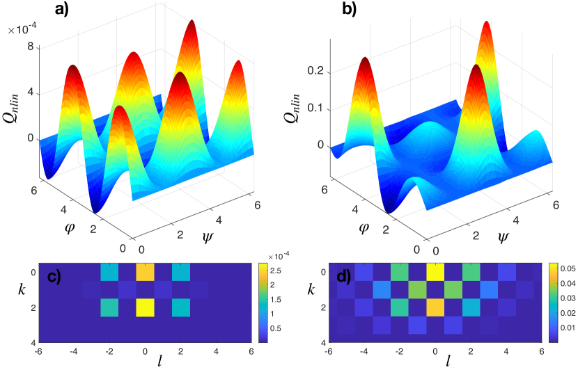
Figure 1: Nonlinear part of the coupling function and the amplitudes of its Fourier modes (see (15)) for $\nu=0.3$ and $\varepsilon=0.05$ (panels (a,c)) and $\varepsilon=0.55$ (panels (b,d)).

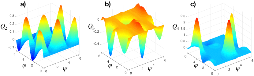
Figure 2: The components $Q_{2,3,4}$ of the nonlinear coupling function for $\nu=0.3$, obtained via a polynomial fit in the range $\varepsilon=0.05,\ldots,0.55$. Comparison with Fig. 1 shows that $Q_{2}$ dominates, as expected, for small $\varepsilon$, while $Q_{4}$ dominates for large $\varepsilon$.

As discussed above, the novel essential feature of the nonlinear coupling function is its dependence on the frequency of the forcing $\nu$. In Fig. 3 we show dependencies of several dominant Fourier modes of the coupling function on parameters $\varepsilon$ and $\nu$.

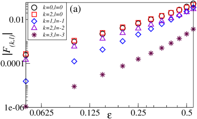
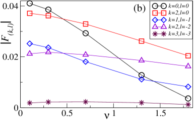
Figure 3: Dependence of amplitudes of different Fourier modes on the amplitude $\varepsilon$ (a) and on the frequency $\nu$ (b) of the forcing.

Next, we analyzed how the nonlinear coupling function varies with the parameter $\mu$. As it follows from the first equation of (7), this parameter determines the radius of the limit cycle oscillation $R_{0}=\sqrt{\mu}$. Furthermore, linearization of this equation yields for a small radius deviation $\delta$ from the limit cycle $\dot{\delta}\approx-2\mu\delta+\varepsilon p(t)\cos\theta$, so that the larger the value of $\mu$, the more stable is the cycle. We computed the nonlinear part of the coupling function for $0.5\leq\mu\leq 3$ and fixed parameters of the forcing, $\nu=0.1$, $\varepsilon=0.4$. (For $\mu<0.5$ the forcing becomes too strong to provide a reliable construction of $Q_{nlin}$.) The results are shown in Fig. 4. One can see that for large $\mu$ the norm of the nonlinear coupling function decays as $\sim\mu^{-2.15}$, what means that the nonlinear effects become less visible in the $\mu\to\infty$ limit, because the linear part decays as $\sim\mu^{-1/2}$.

Figure 4: The norm of the nonlinear coupling function vs. parameter $\mu$ for constant $\varepsilon$ (circles). Bold red line has slope $-2.15$.

Finally, our simulations have shown no essentially interesting dependence on parameter $\alpha\neq 0$, only some quantitative changes.

V.2 Validity of the Winfree and the Kuramoto-Daido forms

While the first-order coupling function for the forcing term adopted in this study can be represented in the Winfree form, this is no more valid for the full nonlinear coupling function. In order to check the validity of the Winfree representation for strong forcing, we estimate an “effective” $Z(\varphi)$ by plotting $\frac{\dot{\varphi}-\omega}{\varepsilon\cos(\nu t)}$ vs $\varphi$ for $\varepsilon\cos(\nu t)>10^{-5}$, cf. Eq. (4). The results for $\varepsilon=0.4$ and three different values of $\nu$ are presented in Fig. 5. For a constant perturbation, $\nu=0$, this approach yields a curve that, as expected, deviates from the linear PRC given by Eq. (10). However, for harmonic driving, the points in the plot do not fall on a curve, what means that in the nonlinear regime the coupling function cannot be decomposed into a product $Z(\varphi)p(\psi)$.

One could find an approximate PRC by averaging the curves in Fig. 5, or by neglecting all the Fourier-components in the expansion (15) except for $l=1$ (and taking only real part of it). In this way one, however, neglects terms that are of the same order of magnitude as the preserved ones.

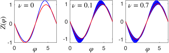
Figure 5: Test for validity of the Winfree form of the phase coupling function, for $\varepsilon=0.4$ and different values of frequency $\nu$. Red lines show the first-order PRC according to Eq. (10).

As was discussed in Section II, there is no unique Kuramoto-Daido model, rather there is a set of models valid for different resonances $\omega/\nu\approx m/n$. The coupling function for the resonance $\omega/\nu\approx m/n$ is obtained from the full coupling function (15) as

$$h_{n,m}(n\varphi-m\psi)=\sum_{k}F_{(kn,-km)}\exp[ikn\varphi-ikm\psi]\;.$$

For example, the main resonance Kuramoto-Daido coupling function $h_{1,1}$ is described by the harmonics $F_{(0,0)},F_{(\pm 1,\mp 1)}$, $F_{(\pm 2,\mp 2)},F_{(\pm 3,\mp 3)},\ldots$ In the first-order approximation one has just the first harmonics terms (12), while for the full nonlinear coupling function also higher-order terms are present for the main resonance. For other resonances, which are not present in the first order, nonlinear coupling provides effective averaged resonant forcing in higher orders in $\varepsilon$. Another way to construct the Kuramoto-Daido model is to perform a direct fit of $\dot{\varphi}-\omega$ vs $(n\varphi-m\psi)\,\text{mod}\,2\pi$ (e.g., representing the function as a Fourier series and finding the Fourier coefficients through minimization of the mean squared error), this approach have been adopted in Ref. Tokuda-Jain-Kiss-Hudson-07 . We illustrate the Kuramoto-Daido coupling functions $h_{1,1}$ and $h_{1,3}$ for $\varepsilon=0.5$ in Fig. 6. While $h_{1,1}$ is rather close to the first-order Kuramoto-Daido model (12), the norm of the coupling for the resonance $1:3$ is rather small.

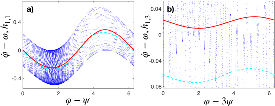
Figure 6: The Kuramoto-Daido models $h(\varphi-\psi)$ constructed for $\varepsilon=0.5$ and $\nu=0.7$ (a) and $h(\varphi-3\psi)$ for $\varepsilon=0.5$, $\nu=0.3$. Blue points show exact values of phase derivative. Solid red and dashed cyan curves are the results of two ways of averaging: the first one is obtained by taking the corresponding diagonal Fourier modes of the reconstructed full coupling function $Q(\varphi,\psi)$, while the second one is obtained via a direct Fourier fit of blue dots.

VI Predicting synchronization regions with nonlinear coupling functions

In this section we demonstrate that the nonlinear phase model can be exploited to predict locking regions, or Arnold tongues. We recall that we cannot construct the coupling function if the system is locked to an external force. However, it does not mean that the phase model is not valid in that parameter domain, but simply that our procedure for the coupling function construction fails. Nevertheless, we can use the coupling function obtained for coupling strength below the synchronization threshold to predict domain of synchrony for stronger forcing (or for other frequencies of the forcing).

For small amplitudes of the forcing, only the main Arnold tongue with $\nu\approx\omega$ is relevant, and it is well captured by the Kuramoto-Daido representation of the phase dynamics in terms of phase differences, cf. Eq. (12). This form of coupling determines the only synchronization domain that has a triangular shape and touches the $\nu$-axis. In the strongly forced regime we can expect appearance of further Arnold tongues. Indeed, the devil’s staircase computed for the full model (7) for $\varepsilon=0.7$, exhibits not only $1:1$ locking but also domains of $1:3$ and $1:2$ synchrony, see Fig. 7.

Now we check how this staircase can be reproduced by the phase model, constructed for $\nu=0.3$, $\varepsilon\leq 0.55$. (We remind that for $\varepsilon>0.55$ the model construction failed because of synchrony.) Combining Eq. (3) with $\dot{\psi}=\nu$ we obtain

$$\frac{\rm d\varphi}{\rm d\psi}=\left(\omega+\varepsilon Q_{1}+\varepsilon^{2}Q_{2}+\varepsilon^{3}Q_{3}+\varepsilon^{4}Q_{4}\right)/\nu\;.$$ (16)

Next, we solve this equation numerically for $\varepsilon=0.7$. Namely, using the Euler technique and precomputed $Q_{2,3,4}$, we find phase increase $\Delta\varphi$ corresponding to a large phase increase $\Delta\psi$ and obtain frequency ratio as $\Delta\varphi/\Delta\psi$. The result is shown in Fig. 7. We see that the phase model obtained for $\nu=0.3$ very well describes the $1:3$ locking domain and the left border of the $1:1$ locking region, but exhibits an essential deviation at the right border of the latter. This can be explained by the frequency dependence of $Q_{nlin}$.

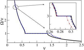
Figure 7: Synchronization domains of the forced SLO with $\varepsilon=0.7$. Black solid line shows the true devil’s staircase and the blue dashed one shows the prediction by the full nonlinear phase model. The red dashed-dotted line is obtained from the integration of the first-order phase approximation (11); one can see that it provides a significantly worse prediction compared to the full model.

As has been discussed above, the Kuramoto-Daido model is expected to be good for small forcing only, because for large forcing the time scale separation between the uniform phase rotation and deviations from it is not valid. Nevertheless, one can formally apply this model and to check quality of predictions of synchronization properties for large forcing amplitudes. We illustrate, how good the model based on the coupling function $h_{1,1}$ predicts the boundaries of the main synchronization region $1:1$ in Fig. 8. One can see that the prediction is quite reasonable, what indicates that for the synchronization properties many nonlinear features of the coupling function are not important. While the Kuramoto-Daido coupling function $h_{1,3}$ (see Fig. 6(b)) correctly predicts existence of the synchronization region $1:3$, its position is strongly shifted in $\nu$ compared to the really observed one, therefore we do not depict it in Fig. 7.

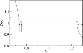
Figure 8: The $1:1$ synchronization domain for the SLO forced with amplitude $\varepsilon=0.5$ and its borders predicted by the Kuramoto-Daido model reconstructed for $\nu=0.7$. The solid curve shows the true locking region. The solid lines with arrows show the borders predicted by the the model obtained from the Fourier coefficients of the coupling function; the dashed lines with arrows show the corresponding prediction of model obtained via direct Fourier fit.

VII Conclusion

In summary, we have presented the concept of a nonlinear phase coupling function for a periodically forced self-sustained oscillator. It generalizes the approach of the phase reduction based on the first order approximation in the forcing strength. For illustration we have chosen the Stuart-Landau oscillator, mainly for the reason of convenience of presentation, because for it the phase and the first-order phase reduction are known analytically. The method can be however straightforwardly applied to other systems, for which the dynamical equations are known. In such a case, the proper phase and its derivative should be determined numerically, see Rosenblum-Pikovsky-19 . The case of a purely observational determination of the nonlinear coupling function (cf. Kralemann_et_al-13 ; RevModPhys.89.045001 ) requires additional efforts, as the reliable methods of the proper phase reconstruction from scalar signals are still missing.

We have demonstrated that the nonlinear coupling function has a shape quite different from that of the first-order approximation, with many more Fourier components present. A novel feature is a dependence of the nonlinear terms on the frequency of the forcing, in contradistinction to the first approximation which is frequency-independent. We have also shown that many differences between the full nonlinear coupling function and its first-order approximation are not so important for determination of the synchronization regions, although the full nonlinear function provides better accuracy.

We foresee that the presented approach can be extended to determination of the phase dynamics of coupled oscillators at strong coupling. An extra problem to be treated here is an additional dependence of the forcing waveform on the strength of the coupling. This study will be reported elsewhere.

The study was supported by the Russian Science Foundation (Grant No. 17-12-01534). We thank S. Schaefer and E. Gengel for useful discussions.

References

- (1) Winfree AT. 1980 The Geometry of Biological Time. Berlin: Springer.
- (2) Kuramoto Y. 1984 Chemical Oscillations, Waves and Turbulence. Berlin: Springer.
- (3) Blekhman I. 1988 Synchronization in Science and Technology. New York: ASME Press.
- (4) Hoppensteadt FC, Izhikevich EM. 1980 Weakly Connected Neural Networks. New York: Springer.
- (5) Pikovsky A, Rosenblum M, Kurths J. 2001 Synchronization. A Universal Concept in Nonlinear Sciences. Cambridge: Cambridge University Press.
- (6) Strogatz SH. 2003 Sync: The Emerging Science of Spontaneous Order. NY: Hyperion.
- (7) Balanov A, Janson N, Postnov D, Sosnovtseva O. 2009 Synchronization: From Simple to Complex. New York: Springer.
- (8) Breakspear M, Heitmann S, Daffertshofer A. 2010 Generative models of cortical oscillations: neurobiological implications of the Kuramoto model. Frontiers in Human Neuroscience 4, 190.
- (9) Richard P, Bakker BM, Teusink B, Dam KV, Westerhoff HV. 1996 Acetaldehyde mediates the synchronization of sustained glycolytic oscillations in population of yeast cells. Eur. J. Biochem. 235, 238–241.
- (10) Strogatz SH, Abrams DM, McRobie A, Eckhardt B, Ott E. 2005 Theoretical mechanics: Crowd synchrony on the Millennium Bridge. Nature 438, 43–44.
- (11) Shim SB, Imboden M, Mohanty P. 2007 Synchronized oscillation in coupled nanomechanical oscillators. Science 316, 95.
- (12) Mondragón-Palomino O, Danino T, Selimkhanov J, Tsimring L, Hasty J. 2011 Entrainment of a population of synthetic genetic oscillators. Science 333, 1315–1319.
- (13) Ermentrout GB, Terman DH. 2010 Mathematical Foundations of Neuroscience. New York: Springer.
- (14) Monga B, Wilson D, Matchen T, Moehlis J. 2019 Phase reduction and phase-based optimal control for biological systems: a tutorial. Biological Cybernetics 113, 11–46.
- (15) Wilson D, Ermentrout B. 2018 Greater accuracy and broadened applicability of phase reduction using isostable coordinates. J. Math. Biology 76, 37–66.
- (16) Rosenblum M, Pikovsky A. 2019 Numerical phase reduction beyond the first order approximation. Chaos 29, 011105.
- (17) Guckenheimer J. 1975 Isochrons and phaseless sets. Journal of Mathematical Biology 1, 259–273.
- (18) Sakaguchi H, Kuramoto Y. 1986 A soluble active rotator model showing phase transition via mutual entrainment. Prog. Theor. Phys. 76, 576–581.
- (19) Daido H. 1992 Order function and macroscopic mutual entrainment in uniformly coupled limit-cycle oscillators. Prog. Theor. Phys. 88, 1213–1218.
- (20) Daido H. 1993 A solvable model of coupled limit-cycle oscillators exhibiting perfect synchrony and novel frequency spectra. Physica D 69, 394–403.
- (21) Daido H. 1996 Onset of cooperative entrainment in limit-cycle oscillators with uniform all-to-all interactions: Bifurcation of the order function. Physica D 91, 24–66.
- (22) Daido H. 1996 Multibranch entrainment and scaling in large populations of coupled oscillators. Phys. Rev. Lett. 77, 1406–1409.
- (23) Nakagawa N, Kuramoto Y. 1993 Collective chaos in a population of globally coupled oscillators. Prog. Theor. Phys. 89, 313–323.
- (24) Nakagawa N, Kuramoto Y. 1994 From collective oscillations to collective chaos in a globally coupled oscillator system. Physica D 75, 74–80.
- (25) Montbrió E, Pazó D. 2011 Shear diversity prevents collective synchronization. Phys. Rev. Lett. 106, 254101.
- (26) Bordyugov G, Pikovsky A, Rosenblum M. 2010 Self-emerging and turbulent chimeras in oscillator chains. Phys. Rev. E 82, 035205.
- (27) Sethia GC, Sen A. 2014 Chimera states: the existence criteria revisited. Phys. Rev. Lett. 112, 144101.
- (28) Rosenblum M, Pikovsky A. 2015 Two types of quasiperiodic partial synchrony in oscillator ensembles. Phys. Rev. E 92, 012919.
- (29) Kralemann B, Frühwirth M, Pikovsky A, Rosenblum M, Kenner T, Schaefer J, Moser M. 2013 In vivo cardiac phase response curve elucidates human respiratory heart rate variability. Nature Communications 4, 2418.
- (30) Tokuda IT, Jain S, Kiss IZ, Hudson JL. 2007 Inferring phase equations from multivariate time series. Phys. Rev. Lett. 99, 064101.
- (31) Stankovski T, Pereira T, McClintock PVE, Stefanovska A. 2017 Coupling functions: Universal insights into dynamical interaction mechanisms. Rev. Mod. Phys. 89, 045001.