A study of coherence based measure of quantumness in (non) Markovian channels

Abstract

We make a detailed analysis of quantumness for various quantum noise channels, both Markovian and non-Markovian. The noise channels considered include dephasing channels like random telegraph noise, non-Markovian dephasing and phase damping, as well as the non-dephasing channels such as generalized amplitude damping and Unruh channels. We make use of a recently introduced witness for quantumness based on the square $l_{1}$ norm of coherence. It is found that the increase in the degree of non-Markovianity increases the quantumness of the channel.

I Introduction

Quantum coherence Hu et al. (2018); Wilde (2013) is central to quantum mechanics, playing a fundamental role for the manifestations of quantum properties of a system. It is at the heart of the phenomena such as multi-particle interference and entanglement which are pivotal for carrying out various quantum information and communication tasks, viz., quantum key distribution Bennett et al. (1992); Grosshans et al. (2003) and teleportation Bennett et al. (1993). An operational formulation of coherence as a resource theory was recently developed Streltsov et al. (2017). The notion of coherence Radhakrishnan et al. (2018) has its roots in quantum optics Glauber (1963); Sudarshan (1963). Recent developments have made use of coherence in superconducting systems Almeida et al. (2013), biological systems Lloyd (2011), non-Markovian phenomena Bhattacharya et al. (2018), foundational issues Singh et al. (2015); Yadin and Vedral (2016) and subatomic physics Alok et al. (2016); Dixit et al. (2019).

Quantum channels are completely positive (CP) and trace preserving maps between the spaces of operators which can transmit classical as well as quantum information. Quantum information protocols are based on the fact that information is transmitted in the form of quantum states. This is achieved either by directly sending non-orthogonal states or by using pre-shared entanglement. The channels can reduce the degree of coherence and entanglement as the information flows from sender to receiver. Interestingly, it was shown in Mani and Karimipour (2015) that quantum channels can have cohering power and that a qubit unitary map has equal cohering and decohering power in any basis. In general, the extent to which the quantum features are affected depends on the underlying dynamics and the type of noise. Therefore it is natural to ask to what extent is coherence preserved by a channel used to transmit quantum information.

The physical foundation of a large number of quantum channels relies on the Born and/or Markov approximations Maniscalco et al. (2007). However, in a number of quantum communication tasks, the characteristic time scales of the system of interest become comparable with the reservoir correlation time. Therefore, a non-Markovian description for such scenarios becomes indispensable Banerjee (2018).

A quantum channel can be used to transport either classical or quantum information. The reliability of a quantum channel is tested by the probability that the output and input states are the same. A well known measure to quantify the performance of a channel is the average fidelity Braunstein et al. (2000); Horodecki et al. (1995, 1996, 1999). The notion of fidelity of two quantum states provides a qualitative measure of their distinguishability Jozsa (1994).

In Shahbeigi and Akhtarshenas (2018), a witness of nonclassicality of a channel was introduced. This is based on average quantum coherence of the state space, using the square $l_{1}$ norm of coherence of qubit channels. It was shown that the extent to which quantum correlation is preserved under local action of the channel cannot exceed the quantumness of the underlying channel.

In this work, we use the definition of quantumness based on the average coherence and apply it to different channels, both Markovian and non-Markovian. Average channel fidelity is a useful figure of merit when considering channel transmission, particularly in the presence of noise. Accordingly, a corresponding study is made on these channels. The paper is organized as follows. In Sec. (II), we briefly review the definition of nonclasscality of quantum channels. Section (III) is devoted to analyzing the interplay of quantumness and average fidelity in various noise models. Results and their discussion is made in Sec (IV). We conclude in Sec. (V).

II Quantum channels and the measure of quantumness

Here, we given a brief overview of quantum channels. This will be followed by a discussion on a coherence based measure of quantumnes of channels.

II.1 Quantum channel

A quantum channel in the Schödinger picture is a completely positive and trace preserving map $\Phi:\mathcal{T}(\mathcal{H}_{A})\rightarrow\mathcal{T}(\mathcal{H}_{B})$, where $\mathcal{H}_{A}$ and $\mathcal{H}_{B}$ are the underlying Hilbert spaces for system $A$ and $B$, respectively. One defines a dual channel, in the Heisenberg picture, as a linear, completely positive map $\Phi^{*}=\mathcal{S}(\mathcal{H}_{A})\rightarrow\mathcal{S}(\mathcal{H}_{B})$. When the input and output systems have equal dimensions ($d_{A}=d_{B}$), $\Phi^{*}$ is also trace-preserving, so that both $\Phi$ and $\Phi^{*}$ are channels in the Schödinger and Heisenberg pictures Holevo (2012).

The operator sum representation of a channel is given as

$$\Phi[\bm{\rho}]=\sum\limits_{\mu}\textbf{M}_{\mu}\bm{\rho}\textbf{M}^{\dagger}_{\mu},$$ (1)

such that the operators $\textbf{M}_{\mu}$, called as Kraus operators, obey the completeness condition, $\sum\limits_{\mu}\textbf{M}_{\mu}^{\dagger}\textbf{M}_{\mu}=\mathbb{1}$. Here, $\mathbb{1}$ is the identity operator. Note that $\bm{\rho}$, in Eq. (1), need not be a pure state. A linear map given in Eq. (1), is called a quantum channel or superoperator (as it maps operators to operators) or completely positive trace preserving (CPTP) map. A quantum channel is characterized by the following properties (i) linearity, i.e., $\Phi[\alpha\bm{\rho}_{1}+\beta\bm{\rho}_{2}]=\alpha\Phi(\bm{\rho}_{1})+\beta\Phi(\bm{\rho}_{2})$, where $\alpha$ and $\beta$ are complex number, (ii) Hermiticity preserving, i.e., $\bm{\rho}=\bm{\rho}^{\dagger}\implies\Phi[\bm{\rho}]=\Phi[\bm{\rho}]^{\dagger}$, (iii) positivity preserving, i.e., $\bm{\rho}\geq 0\implies\Phi[\bm{\rho}]\geq 0$, and (iv) trace preserving, i.e., $Tr(\Phi[\bm{\rho}])=Tr(\bm{\rho})$.

II.2 A coherence based measure of quantumness of channels

A coherence based measure was introduced in Shahbeigi and Akhtarshenas (2018)

$$Q_{C}(\Phi)=N_{C}\int C(\Phi(\rho))d\mu(\rho).$$ (2)

Here, $\Phi$ is the channel under consideration, $C$ denotes the chosen measure of coherence and $N_{C}$ is a normalization constant. To proceed, we analyze the effect of a qubit channel on a state $\bm{\rho}=\frac{1}{2}(\bm{I}+\bm{\xi}\bm{\sigma})$. This turns out to be a affine transformation on a Bloch sphere, such that the Bloch vector $\xi$ transforms as

$$\Phi(\bm{\rho})=\bm{\rho}^{\prime}=\frac{1}{2}(\bm{I}+\bm{\xi}^{\prime}\bm{\sigma}).$$ (3)

Here, $\bm{\xi}^{\prime}=\bm{A}\bm{\xi}+\bm{B}$, such that the matrices $\textbf{A}_{3\times 3}$ and $\textbf{B}_{3\times 1}$ depend on the channel parameters. By choosing the square $l_{1}$-norm as the measure of coherence, we compute the coherence with respect to an arbitrary orthonormal basis. To make the quantumness witness a basis independent quantity, one performs optimization over all orthonormal basis, leading to a closed expression for the quantumness witness

$$Q_{C_{l_{1}}^{2}}(\Phi)=\lambda_{2}+\lambda_{3}.$$ (4)

Here, $\lambda_{1}\geq\lambda_{2}\geq\lambda_{3}$ are eigenvalues of matrix $\bm{\mathcal{L}}=\frac{1}{2}(\bm{A}\bm{A}^{T}+5\bm{B}\bm{B}^{T})$, with $T$ denoting the transpose operation. Thus, Eq. (4) gives an operational definition of the quantumness of a channel. In what follows, we will drop the subscript $C_{l_{1}}^{2}$ and call the quantumness of a map $\Phi$ just as $Q(\Phi)$. It is worth mentioning here, that for the unital channels, which map identity to identity, i.e., $\Phi(\bm{I})=\bm{I}$, the above definition of quantumness coincides with the geometric discord Shahbeigi and Akhtarshenas (2018).

III Specific channels

In this section, we give a brief account of various quantum channels Nielsen and Chuang (2002); Watrous (2018) used in this work. The dephasing class includes random telegraph noise (RTN) Daffer et al. (2004); Kumar et al. (2018); Banerjee et al. (2017), non-Markovian dephasing (NMD) Shrikant et al. (2018) and phase damping (PD) Banerjee and Ghosh (2007) channels while in the non-dephasing class, we consider generalized amplitude damping (GAD) Srikanth and Banerjee (2008); Omkar et al. (2013) and Unruh channels Omkar et al. (2016).

Random Telegraph Noise: This channel characterizes the dynamics when the system is subjected to a bi-fluctuating classical noise, generating RTN with pure dephasing. The dynamical map acts as follows

$$\Phi^{RTN}(\bm{\rho})=\bm{\mathcal{R}}_{0}\bm{\rho}\bm{\mathcal{R}}_{0}^{\dagger}+\bm{\mathcal{R}}_{1}\bm{\rho}\bm{\mathcal{R}}_{1}^{\dagger},$$ (5)

where the two Kraus operators are given by

$$\bm{\mathcal{R}}_{0}=\sqrt{\frac{1+\Lambda(t)}{2}}\bm{I},\qquad\bm{\mathcal{R}}_{1}=\sqrt{\frac{1-\Lambda(t)}{2}}\bm{\sigma}_{z}.$$ (6)

Here, $\Lambda(t)$ is the memory kenel

$$\Lambda(t)=e^{-\gamma t}\Bigg{[}\cos\Big{[}\sqrt{\big{(}\frac{2b}{\gamma}\big{)}^{2}-1}~{}\gamma t\Big{]}+\frac{\sin\Big{[}\sqrt{\big{(}\frac{2b}{\gamma}\big{)}^{2}-1}~{}\gamma t\Big{]}}{\sqrt{\big{(}\frac{2b}{\gamma}\big{)}^{2}-1}}\Bigg{]},$$ (7)

where $b$ quantifies the system-environment coupling strength and $\gamma$ is proportional to the fluctuation rate of the RTN. Also, $\bm{I}$ and $\bm{\sigma}_{z}$ are the identity and Pauli spin matrices, respectively. The completeness condition reads $\bm{\mathcal{R}}_{0}\bm{\mathcal{R}}_{0}^{\dagger}+\bm{\mathcal{R}}_{1}\bm{\mathcal{R}}_{1}^{\dagger}=\bm{I}$. The dynamics is Markovian [non-Markovian] if $(4b\uptau)^{2}>1~{}[(4b\uptau)^{2}<1]$, where $\uptau=1/(2\gamma)$. Starting with the state $\bm{\rho}=\frac{1}{2}(\bm{I}+\bm{\xi}\bm{\sigma})$, the new Bloch vector is given by $\bm{\xi}^{\prime}=[\bm{\xi}_{x}\Lambda(t),\bm{\xi}_{y}\Lambda(t),\bm{\xi}_{z}]^{T}$. This implies $\bm{A}={\rm diag.}[\Lambda(t),\Lambda(t),1]$ and $\bm{B}=0$, and consequently, $\bm{\mathcal{L}}={\rm diag.}[\frac{1}{2}[\Lambda(t)]^{2},\frac{1}{2}[\Lambda(t)]^{2},\frac{1}{2}]$. Since, $-1\leq\Lambda(t)\leq 1$, we identify both the small eigenvalues as $\frac{1}{2}[\Lambda(t)]^{2}$, leading to

$$Q(\Phi^{RTN})=[\Lambda(t)]^{2}.$$ (8)

We, next compute the fidelity for the states $\bm{\rho}$ and $\bm{\rho}^{\prime}$ and study its interplay with quantumness. The fidelity between qubit states $\bm{\rho}$ and $\bm{\rho}^{\prime}$ is

$$F(\bm{\rho},\bm{\rho}^{\prime})=Tr[\bm{\rho}\bm{\rho}^{\prime}]+2\sqrt{Det[\bm{\rho}]Det[\bm{\rho}^{\prime}]}.$$ (9)

Using a general qubit parametrization

$$\bm{\rho}=\begin{bmatrix}\cos^{2}(\theta/2)&\frac{1}{2}e^{-i\phi}\sin(\theta)\\ \frac{1}{2}e^{i\phi}\sin(\theta)&\sin^{2}(\theta/2)\end{bmatrix},$$ (10)

the fidelity for RTN model turns out to be

$$F_{RTN}=\frac{1}{4}\big{[}3+\cos(2\theta)+2\sin^{2}(\theta)\Lambda(t)\big{]}.$$ (11)

In order to make this quantity state independent, we calculate the average fidelity $\mathcal{F}=\frac{1}{4\pi}\int_{0}^{2\pi}\int_{0}^{\pi}F\sin(\theta)d\theta d\phi$. We have

$$\mathcal{F}_{RTN}=\frac{1}{3}[2+\Lambda(t)].$$ (12)

Since $-1\leq\Lambda(t)\leq 1$, the average fidelity is symmetric about its classical value $2/3$.

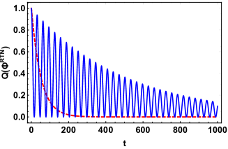
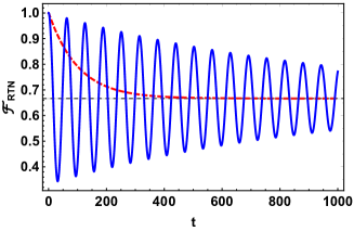
Figure 1: RTN channel: The quantumness $Q(\Phi^{RTN})$ Eq. (8) and average fidelity $\mathcal{F}_{RTN}$ Eq. (12), plotted with respect to time $t$ (sec.), for a qubit subjected to RTN. The solid (blue) and dashed (red) curves correspond to non-Markovian ($b=0.05,~{}\gamma=0.001$) and Markovian ($b=0.07,~{}\gamma$) cases, respectively. The fidelity oscillates symmetrically about $2/3$ in non-Markovian case, while in Markovian case, it decreases monotonically and saturates to this value.

Non-Markovian dephasing: This channel is an extension of the dephasing channel to non-Markovian class. The non-Markovianity is identified with the breakdown in complete-positivity of the map. The Kraus operators are given by

$$\bm{\mathcal{N}}_{0} =\sqrt{(1-\alpha p)(1-p)}~{}\bm{I},$$

$${\rm and}~{}~{}~{}\bm{\mathcal{N}}_{1} =\sqrt{p+\alpha p(1-p)}~{}\bm{\sigma}_{z}.$$ (13)

Here, the parameter $\alpha$ quantifies the degree of non-Markovianity of the channel and $p$ is a time-like parameter such that $0\leq p\leq 1/2$. In this case, the quantumness parameter turns out to be

$$Q(\Phi^{NMD})=\Omega^{2}(p),$$ (14)

where $\Omega=1-2p-2\alpha p(1-p)$. The average fidelity, in this case, is given by

$$\mathcal{F}_{NMD}=\frac{1}{3}[2+\Omega(p)].$$ (15)

We use the parametrization $p=\frac{1}{2}(1-e^{-\kappa t})$, such that as $t:0\rightarrow\infty$, $p:0\rightarrow 1/2$.

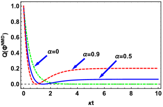
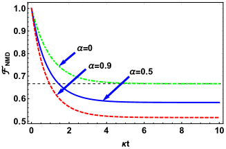
Figure 2: NMD channel: The quantumness $Q(\Phi^{NMD})$ Eq. (14) and average fidelity $\mathcal{F}_{NMD}$ Eq. (15), plotted with respect to the dimensionless parameter $\kappa t$, for a qubit subjected to NMD, for different values of parameter $\alpha$.

Phase damping (PD) channel: PD channel models the phenomena where decoherence occurs without dissipation (loss of energy). The dynamical map, in this case has the Kraus representation

$$\bm{\mathcal{P}}_{0}=\begin{bmatrix}1&0\\ 0&\sqrt{1-S}\end{bmatrix},\qquad\bm{\mathcal{P}}_{1}=\begin{bmatrix}0&0\\ 0&\sqrt{S}\end{bmatrix}.$$ (16)

The parameter $S$ can be modeled by the following time dependence $S=1-\cos^{2}(\chi t)$, for $0\leq\chi t\leq\pi/2$. The quantumness parameter, in this case, is given by

$$Q(\Phi^{PD})=1-S=\cos^{2}(\chi t).$$ (17)

The average fidelity turns out to be

$$\mathcal{F}_{PD}=\frac{1}{3}[2+\cos(\chi t)].$$ (18)

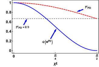
Figure 3: PD channel: The quantumness $Q(\Phi^{PD})$ Eq. (17) and average fidelity $\mathcal{F}_{PD}$ Eq. (18), plotted with respect to the dimensionless quantity $\chi t$, for a qubit subjected to PD noise.

Generalized Amplitude Damping (GAD) channel: GAD is a generalization of the AD channel to finite temperatures Banerjee (2018). The later models processes like spontaneous emission from an atom and is pertinent to the problem of quantum erasure Srikanth and Banerjee (2007). The dynamics, in this case, is governed by the following Kraus operators

$$\bm{\mathcal{A}}_{0} =\begin{bmatrix}\sqrt{\Theta}&0\\ 0&\sqrt{s\Theta}\end{bmatrix},\quad\bm{\mathcal{A}}_{1}=\begin{bmatrix}0&\sqrt{p\Theta}\\ 0&0\end{bmatrix},$$

$$\bm{\mathcal{A}}_{2} =\begin{bmatrix}\sqrt{s(1-\Theta)}&0\\ 0&\sqrt{(1-\Theta)}\end{bmatrix},\quad\bm{\mathcal{A}}_{3}=\begin{bmatrix}0&0\\ \sqrt{p(1-\Theta)}&0\end{bmatrix}.$$ (19)

Here, $\Theta=\frac{n+1}{2n+1}$, and $s=\exp[-\frac{\gamma t}{2}(2n+1)]$. Also, $n$ is the mean number of excitations in the bath and $\gamma$ represents the spontaneous emission rate. In the zero temperature limit, $n=0$, implying $\Theta=1$, thereby recovering the AD channel. The quantumness parameter for GAD channel comes out to be

$$Q(\Phi^{GAD})=\begin{cases}\frac{1}{2}s+\tilde{s}&{\rm for}~{}~{}t\leq\tau,\\ \\ s&{\rm for}~{}~{}t>\tau.\end{cases}$$ (20)

with,

$$\tilde{s} =\frac{5}{2}(2\Theta-1)^{2}(1-s)^{2},$$

$$\tau =-\frac{2}{\gamma(2n+1)}\ln\bigg{[}\frac{5}{6+4n+n^{2}}\bigg{]}.$$

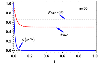
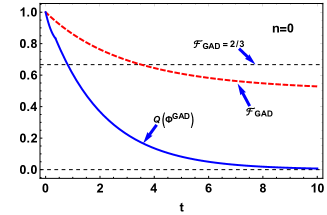
Figure 4: GAD channel: The quantumness $Q(\Phi^{GAD})$ Eq. (20) and fidelity $\mathcal{F}_{GAD}$ Eq. (21), plotted with respect to time $t$ (sec.), for a qubit subjected to GAD noise. With $\gamma=1$, the top and bottom panels correspond to the cases when $n=50$ and $0$, respectively. Here, $\tau\approx 0.1246$ and $0.3646$ in the former and later case, respectively . The $n=0$ case corresponds to the zero temperature limit, such that GAD reduces to AD noise.

The average fidelity in this case is given by

$$\mathcal{F}_{GAD}=\frac{1}{6}[3+2\sqrt{s}+s].$$ (21)

Here $s=\exp[-\frac{\gamma t}{2}(2n+1)]$.

Unruh channel: To an observer undergoing acceleration $a$, the Minkowski vacuum appears as a warm gas emitting black-body radiation at temperature given by $T=\frac{\hbar a}{2\pi cK_{B}}$, called the Unruh temperature and the effect is known as the Unruh effect. The Unruh effect has been described as a noisy quantum channel with the following Kraus operators

$$\mathbf{U}_{0}=\begin{bmatrix}\cos(r)&0\\ 0&1\end{bmatrix}\qquad{\rm and}\qquad\mathbf{U}_{1}=\begin{bmatrix}0&0\\ \sin(r)&0\end{bmatrix}.$$ (22)

Here, $\cos(r)=[1+\exp(-2\pi c\omega/{\rm a})]^{-1/2}$. The quantumness parameter for the Unruh channel turns out to be

$$Q(\Phi^{{\rm Unruh}})=\cos^{2}(r).$$ (23)

The average fidelity here is

$$\mathcal{F}_{{\rm Unruh}} =\frac{1}{12}(4\cos(r)+\cos(2r)+7).$$ (24)

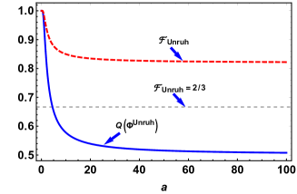
Figure 5: Unruh channel: The behavior of quantumness and average fidelity depicted with respect to the acceleration a (in units $\hbar=c=1$).

IV Results and discussion

The quantumness of noisy channels is quantified by the coherence measure given by Eq. (2). For specific case of a two level system (qubit), using square $l_{1}$ norm as a measure of coherence, one obtains a simple working rule for computing the quantumness of a channel, given in Eq. (4).

For RTN channel, the quantumness measure turns out to be the square of the memory kernel $\Lambda(t)$, defined in Eq. (7). In the non-Markovian regime, both the quantumness as well as fidelity are seen to sustain much longer in time as compared with the Markovian case, Fig. 1. In the limit $t\rightarrow\infty$, $\Lambda(t)\rightarrow 0$, consequently, we have

$$Q(\Phi^{RTN})=\Lambda^{2}(t)\rightarrow 0,~{}~{}{\rm and}~{}~{}\mathcal{F}_{RTN}=\frac{1}{3}(2+\Lambda(t))\rightarrow\frac{2}{3}.$$ (25)

This is consistent with our notion of fidelity less than or equal to $2/3$ for a processes that can be simulated by a classical theory. The NMD channel shows non-zero quantumness within the allowed range, i.e., $[0,1/2]$, of time like parameter $p$, for $0<\alpha\leq 1$. In this case, the parameter $\alpha$ quantifies the degree of non-Markovianity, which increases as $\alpha$ goes from $0$ to $1$. At $p=1/2$, i.e., for $t\rightarrow\infty$, $\Omega(p)=-\alpha/2$, we have

$$Q(\Phi^{NMD})=\alpha^{2}/4\quad{\rm and}\quad\mathcal{F}_{NMD}=\frac{2}{3}(1-\alpha/2)$$ (26)

That is, the quantumness parameter is always positive but the average fidelity goes below its classical limit. This is consistent with Shahbeigi and Akhtarshenas (2018) that a nonzero value of the coherence based measure of quantumness is a necessary but not sufficient criterion for quantum advantage in teleportation fidelity. However, in the Markovian limit, i.e., $\alpha\rightarrow 0$, $\Omega\rightarrow 1-2p$. Since $p\in[0,1/2]$, implies $\Omega\in[0,1]$. Therefore, $Q(\Phi^{NMD})=(1-2p)^{2}$ and $\mathcal{F}_{NMD}=\frac{1}{3}[2+(1-2p)]$, both the quantities lead to similar predictions in this limit. These features are depicted in Fig. 2.

One of the purely quantum noise channels is the PD channel which characterizes the processes accompanied with the loss of coherence without loss of energy. The behavior of quantumness and average fidelity, in this case, is depicted in Fig 3. The parameter $Q(\Phi^{PD})$ becomes zero as $\mathcal{F}_{PD}$ reaches $2/3$.

Next we analyzed non-dephasing models such as GAD and Unruh channels. From the GAD channel, one can recover the AD channel in the zero temperature limit, i.e., when $n=0$, see Eq. (III). In this case $\Theta=1$ and the quantumness parameter, with $\xi=1-s$, becomes

$$Q(\Phi^{AD})=\begin{cases}\frac{1}{2}[6\xi^{2}-3\xi+2]&{\rm for}~{}~{}\xi\leq 1/6,\\ \\ 1-\xi&{\rm for}~{}~{}\xi>1/6.\end{cases}$$ (27)

This is consistent with the results given in Shahbeigi and Akhtarshenas (2018). In the case of GAD channel, the quantumness parameter is nonzero even though the average fidelity goes below its classical limit $2/3$. This reiterates the statement made earlier regarding quantumness and average teleportation fidelity, Fig. 4. In the high temperature regime, both the measures, i.e., quantumness as well as average fidelity seem to lead to similar predictions at the same time. For Unruh channel, the quantumness and average fidelity are studied with respect to the acceleration $a$. Both the measures show a saturation at values which are well above their classical limits, Fig 5. This is in consonance with Omkar et al. (2016), where it was shown that the Unruh channel, though structurally similar to the AD channel, is different from it.

V Conclusion

We studied the quantumness and average fidelity of various channels, both Markovian as well as non-Markovian. Specifically, we considered the dephasing channels like RTN, NMD and PD channels and non-dephasing channels such as GAD and Unruh channels. The non-Markovian dynamics (exhibited by RTN and NMD channels in this case) is found to favor the nonclassicality. This is explicitly seen from the fact that a nonzero value of parameters controlling the degree of non-Markovianity takes the quantumness beyond the classical value. The non-Markovianity assisted enhancement of nonclassicality can be of profound importance in carrying out quantum information tasks. This can be realized by effectively engineering the system-reservoir models. The quantumness measure and average fidelity exhibit similar predictions for the Unruh channel. Similar behavior is observed for the dephasing channels, albeit, in the Markovian regime. This can bee seen in RTN and NMD channels. In contrast, in the non-dephasing Lindbladian channel, considered here, the quantumness witness and average fidelity show qualitatively similar results.

Such a study of the interplay between nonclassicality of the quantum channels with the underlying dynamics can be useful from the quantum information point of view, and also brings out the effectiveness of the measure of quantumness under different types of dynamics.

References

- Hu et al. (2018) M.-L. Hu, X. Hu, J. Wang, Y. Peng, Y.-R. Zhang, and H. Fan, Physics Reports (2018).
- Wilde (2013) M. M. Wilde, Quantum information theory (Cambridge University Press, 2013).
- Bennett et al. (1992) C. H. Bennett, F. Bessette, G. Brassard, L. Salvail, and J. Smolin, Journal of cryptology 5, 3 (1992).
- Grosshans et al. (2003) F. Grosshans, G. Van Assche, J. Wenger, R. Brouri, N. J. Cerf, and P. Grangier, Nature 421, 238 (2003).
- Bennett et al. (1993) C. H. Bennett, G. Brassard, C. Crépeau, R. Jozsa, A. Peres, and W. K. Wootters, Phys. Rev. Lett. 70, 1895 (1993), URL https://link.aps.org/doi/10.1103/PhysRevLett.70.1895.
- Streltsov et al. (2017) A. Streltsov, G. Adesso, and M. B. Plenio, Reviews of Modern Physics 89, 041003 (2017).
- Radhakrishnan et al. (2018) C. Radhakrishnan, Z. Ding, F. Shi, J. Du, and T. Byrnes, arXiv preprint arXiv:1805.09263 (2018).
- Glauber (1963) R. J. Glauber, Phys. Rev. 131, 2766 (1963), URL https://link.aps.org/doi/10.1103/PhysRev.131.2766.
- Sudarshan (1963) E. C. G. Sudarshan, Phys. Rev. Lett. 10, 277 (1963), URL https://link.aps.org/doi/10.1103/PhysRevLett.10.277.
- Almeida et al. (2013) J. Almeida, P. C. De Groot, S. Huelga, A. Liguori, and M. B. Plenio, Journal of Physics B: Atomic, Molecular and Optical Physics 46, 104002 (2013).
- Lloyd (2011) S. Lloyd, in Journal of Physics: Conference Series (IOP Publishing, 2011), vol. 302, p. 012037.
- Bhattacharya et al. (2018) S. Bhattacharya, S. Banerjee, and A. K. Pati, Quantum Information Processing 17, 236 (2018).
- Singh et al. (2015) U. Singh, M. N. Bera, H. S. Dhar, and A. K. Pati, Phys. Rev. A 91, 052115 (2015), URL https://link.aps.org/doi/10.1103/PhysRevA.91.052115.
- Yadin and Vedral (2016) B. Yadin and V. Vedral, Physical Review A 93, 022122 (2016).
- Alok et al. (2016) A. K. Alok, S. Banerjee, and S. U. Sankar, Nuclear Physics B 909, 65 (2016).
- Dixit et al. (2019) K. Dixit, J. Naikoo, S. Banerjee, and A. K. Alok, The European Physical Journal C 79, 96 (2019).
- Mani and Karimipour (2015) A. Mani and V. Karimipour, Phys. Rev. A 92, 032331 (2015), URL https://link.aps.org/doi/10.1103/PhysRevA.92.032331.
- Maniscalco et al. (2007) S. Maniscalco, S. Olivares, and M. G. A. Paris, Phys. Rev. A 75, 062119 (2007), URL https://link.aps.org/doi/10.1103/PhysRevA.75.062119.
- Banerjee (2018) S. Banerjee, Open Quantum Systems: Dynamics of Nonclassical Evolution (Springer, 2018).
- Braunstein et al. (2000) S. L. Braunstein, C. A. Fuchs, and H. J. Kimble, Journal of Modern Optics 47, 267 (2000).
- Horodecki et al. (1995) R. Horodecki, P. Horodecki, and M. Horodecki, Physics Letters A 200, 340 (1995).
- Horodecki et al. (1996) R. Horodecki, M. Horodecki, and P. Horodecki, Physics Letters A 222, 21 (1996).
- Horodecki et al. (1999) M. Horodecki, P. Horodecki, and R. Horodecki, Physical Review A 60, 1888 (1999).
- Jozsa (1994) R. Jozsa, Journal of modern optics 41, 2315 (1994).
- Shahbeigi and Akhtarshenas (2018) F. Shahbeigi and S. J. Akhtarshenas, Phys. Rev. A 98, 042313 (2018), URL https://link.aps.org/doi/10.1103/PhysRevA.98.042313.
- Holevo (2012) A. S. Holevo, Quantum systems, channels, information: a mathematical introduction, vol. 16 (Walter de Gruyter, 2012).
- Nielsen and Chuang (2002) M. A. Nielsen and I. Chuang, Quantum computation and quantum information (2002).
- Watrous (2018) J. Watrous, The theory of quantum information (Cambridge University Press, 2018).
- Daffer et al. (2004) S. Daffer, K. Wódkiewicz, J. D. Cresser, and J. K. McIver, Phys. Rev. A 70, 010304 (2004), URL https://link.aps.org/doi/10.1103/PhysRevA.70.010304.
- Kumar et al. (2018) N. P. Kumar, S. Banerjee, R. Srikanth, V. Jagadish, and F. Petruccione, Open Systems and Information Dynamics 25, 1850014 (2018), eprint 1711.03267.
- Banerjee et al. (2017) S. Banerjee, N. P. Kumar, R. Srikanth, V. Jagadish, and F. Petruccione, arXiv:1703.08004 (2017).
- Shrikant et al. (2018) U. Shrikant, R. Srikanth, and S. Banerjee, Physical Review A 98, 032328 (2018).
- Banerjee and Ghosh (2007) S. Banerjee and R. Ghosh, Journal of Physics A: Mathematical and Theoretical 40, 13735 (2007).
- Srikanth and Banerjee (2008) R. Srikanth and S. Banerjee, Physical Review A 77, 012318 (2008).
- Omkar et al. (2013) S. Omkar, R. Srikanth, and S. Banerjee, Quantum information processing 12, 3725 (2013).
- Omkar et al. (2016) S. Omkar, S. Banerjee, R. Srikanth, and A. K. Alok, Quantum Inf. and Comp. 16 (2016).
- Srikanth and Banerjee (2007) R. Srikanth and S. Banerjee, Physics Letters A 367, 295 (2007).