Compositional Synthesis of Symbolic Models for Networks of Switched Systems^∗

Abstract.

In this paper, we provide a compositional methodology for constructing symbolic models for networks of discrete-time switched systems. We first define a notion of so-called augmented-storage functions to relate switched subsystems and their symbolic models. Then we show that if some dissipativity type conditions are satisfied, one can establish a notion of so-called alternating simulation function as a relation between a network of symbolic models and that of switched subsystems. The alternating simulation function provides an upper bound for the mismatch between the output behavior of the interconnection of switched subsystems and that of their symbolic models. Moreover, we provide an approach to construct symbolic models for discrete-time switched subsystems under some assumptions ensuring incremental passivity of each mode of switched subsystems. Finally, we illustrate the effectiveness of our results through two examples.

1. Introduction

The notion of symbolic models (a.k.a. finite abstractions) plays an important role in the control of hybrid systems (see [Tab09] and the references therein). Symbolic models allow us to use automata-theoretic methods [MPS95] to design controllers for hybrid systems with respect to logic specifications such as those expressed as linear temporal logic (LTL) formulae [BK08]. Symbolic models are established for incrementally stable switched systems, a class of hybrid systems [Lib03], by providing approximate bisimulation relations between them [GPT10, GGM16, SG17, CGG13]. However, as the complexity of constructing symbolic models grows exponentially in the number of state variables in the concrete system, the approaches proposed in [GPT10, GGM16, SG17] limit the application of symbolic models to only low-dimensional switched systems. Although the result in [CGG13] provides a state-space discretization-free approach for computing symbolic models of incrementally stable switched systems, this approach is still monolithic and reduces the computational complexity only for switched systems with few modes, see [CGG13, Section IV(D)].

Motivated by the above limitation, in this work we aim at proposing a compositional framework for constructing symbolic models for interconnected switched systems. To do so, we first $i)$ partition the overall concrete switched system into a number of concrete switched subsystems and construct symbolic models of them individually; $ii)$ then establish a compositional scheme that allows us to construct a symbolic models of the overall network using those individual ones.

The compositional framework based on a divide-and-conquer scheme [Kea11] is not new. Several results have already introduced compositional techniques for constructing symbolic models of networks of control subsystems. The results in [TI08, PPB16, MSSM18, SGZ18, SZ18] provide techniques to approximate networks of control subsystems by networks of symbolic models by assuming some stability property of the concrete subsystems. Other compositional approaches provide techniques to design symbolic models of concrete networks without requiring any stability property or condition on the gains of subsystems [MGW17, HAT17, KAZ18]. However, none of the aforementioned results in [TI08, PPB16, MSSM18, SGZ18, SZ18, MGW17, HAT17, KAZ18] provide a compositional framework for constructing symbolic models for interconnected switched systems.

In this paper, we provide a compositional methodology for the construction of symbolic models of interconnected switched systems based on dissipativity theory [AMP16]. We first define a notion of so-called augmented-storage functions to relate switched subsystems and their symbolic models. Then, by leveraging dissipativity-type compositional conditions, we construct a notion of so-called alternating simulation functions as a relation between the interconnection of switched subsystems and that of their symbolic models. This alternating simulation function allows one to determine quantitatively the mismatch between the output behavior of the interconnection of switched subsystems and that of their symbolic models. Moreover, we provide an approach to construct symbolic models together with their corresponding augmented-storage functions for discrete-time switched subsystems under some assumptions ensuring incremental passivity of each mode of switched subsystems. Finally, we apply our results to a model of road traffic by constructing compositionally a symbolic model of a network containing $50$ cells of $1000$ meters each. We also design controllers compositionally maintaining the density of traffic lower than $30$ vehicles per cell. Additionally, we apply our results to an interconnection of switched subsystems admitting multiple incrementally passive storage functions.

The results presented in this paper are mainly concerned with the compositional construction of symbolic models of interconnected discrete-time switched systems. The constructed symbolic models here can be used to synthesize controllers monolithically or also compositionally. Compositional approaches for controller synthesis can be found in [PPB18, MGW17] and references therein.

2. Notation and Preliminaries

2.1. Notation

We denote by $\mathbb{R}$, $\mathbb{Z}$, and $\mathbb{N}$ the set of real numbers, integers, and non-negative integers, respectively. These symbols are annotated with subscripts to restrict them in the obvious way, e.g., $\mathbb{R}_{>0}$ denotes the positive real numbers. Given $N\in\mathbb{N}_{\geq 1}$, vectors $\nu_{i}\in\mathbb{R}^{n_{i}}$, $n_{i}\in\mathbb{N}_{\geq 1}$, and $i\in[1;N]$, we use $\nu=[\nu_{1};\ldots;\nu_{N}]$ to denote the vector in $\mathbb{R}^{n}$ with $n=\sum_{i}n_{i}$ consisting of the concatenation of vectors $\nu_{i}$. The closed interval in $\mathbb{N}$ is denoted by $[a;b]$ for $a,b\in\mathbb{N}$ and $a\leq b$. We denote by $\mathsf{diag}(A_{1},\ldots,A_{N})$ the block diagonal matrix with diagonal matrix entries $A_{1},\ldots,A_{N}$. We denote the identity matrix in $\mathbb{R}^{n\times n}$ by $I_{n}$. The individual elements in a matrix $A\in\mathbb{R}^{m\times n}$, are denoted by $\{A\}_{ij}$, where $i\in[1;m]$ and $j\in[1;n]$. We denote by $\left\|\cdot\right\|$ the infinity norm. We denote by $|\cdot|$ the cardinality of a given set and by ${\varnothing}$ the empty set. For any set $S\subseteq\mathbb{R}^{n}$ of the form of finite union of boxes, e.g., $S=\bigcup_{j=1}^{M}S_{j}$ for some $M\in\mathbb{N}$, where $S_{j}=\prod_{i=1}^{n}[c_{i}^{j},d_{i}^{j}]\subseteq\mathbb{R}^{n}$ with $c^{j}_{i}<d^{j}_{i}$, and positive constant $\eta\leq\emph{span}(S)$, where $\emph{span}(S)=\min_{j=1,\ldots,M}\eta_{S_{j}}$ and $\eta_{S_{j}}=\min\{|d_{1}^{j}-c_{1}^{j}|,\ldots,|d_{n}^{j}-c_{n}^{j}|\}$, we define $[S]_{\eta}=\{a\in S\,\,|\,\,a_{i}=k_{i}\eta,k_{i}\in\mathbb{Z},i=1,\ldots,n\}$. The set $[S]_{\eta}$ will be used as a finite approximation of the set $S$ with precision $\eta$. Note that $[S]_{\eta}\neq{\varnothing}$ for any $\eta\leq\emph{span}(S)$. We use notations $\mathcal{K}$ and $\mathcal{K}_{\infty}$ to denote different classes of comparison functions, as follows: $\mathcal{K}=\{\alpha:\mathbb{R}_{\geq 0}\rightarrow\mathbb{R}_{\geq 0}|$ $\alpha$ is continuous, strictly increasing, and $\alpha(0)=0\}$; $\mathcal{K}_{\infty}=\{\alpha\in\mathcal{K}|$ $\lim\limits_{r\rightarrow\infty}\alpha(r)=\infty\}$.

2.2. Discrete-Time Switched and Transition Systems

In this work we consider discrete-time switched systems of the following form.

Definition 1.

A discrete-time switched system $\Sigma$ is defined by the tuple $\Sigma=(\mathbb{X},P,\mathbb{W},F,\mathbb{Y}_{1},\mathbb{Y}_{2},h_{1},h_{2})$, where

• $\mathbb{X},\mathbb{W},\mathbb{Y}_{1}$, and $\mathbb{Y}_{2}$ are the state set, internal input set, external output set, and internal output set, respectively, and are assumed to be subsets of normed vector spaces with appropriate finite dimensions;

• $P=\{1\cdots,m\}$ is the finite set of modes;

• $F=\{f_{1},\cdots,f_{m}\}$ is a collection of set-valued maps $f_{p}:\mathbb{X}\times\mathbb{W}\rightrightarrows\mathbb{X}$ for all $p\in P$;

• $h_{1}:\mathbb{X}\rightarrow\mathbb{Y}_{1}$ is the external output map.

• $h_{2}:\mathbb{X}\rightarrow\mathbb{Y}_{2}$ is the internal output map.

The discrete-time switched system $\Sigma$ is described by difference inclusions of the form

$$\Sigma:\left\{\begin{array}[]{rl}\mathbf{x}(k+1)&\!\!\!\!\in f_{\mathsf{p}(k)}(\mathbf{x}(k),\omega(k)),\\ \mathbf{y}_{1}(k)&\!\!\!\!=h_{1}(\mathbf{x}(k)),\\ \mathbf{y}_{2}(k)&\!\!\!\!=h_{2}(\mathbf{x}(k)),\end{array}\right.$$ (4)

where $\mathbf{x}:\mathbb{N}\rightarrow\mathbb{X}$, $\mathbf{y}_{1}:\mathbb{N}\rightarrow\mathbb{Y}_{1}$, $\mathbf{y}_{2}:\mathbb{N}\rightarrow\mathbb{Y}_{2}$, $\mathsf{p}:\mathbb{N}\rightarrow P$, and $\omega:\mathbb{N}\rightarrow\mathbb{W}$ are the state signal, external output signal, internal output signal, switching signal, and internal input signal, respectively. We denote by $\Sigma_{p}$ the system in (4) with constant switching signal $\mathsf{p}(k)=p\in P~{}\forall k\in\mathbb{N}$. We use $\mathbf{X}_{x_{0},\overline{p},\overline{\omega}}$ and $\mathbf{Y}_{x_{0},\overline{p},\overline{\omega}}$ to denote the sets of infinite state and external output runs of $\Sigma$, respectively, associated with infinite switching sequence $\overline{p}=\{p_{0},p_{1},\ldots\}$, infinite internal input sequence $\overline{\omega}=\{w_{0},w_{1},\ldots\}$, and initial state $x_{0}\in\mathbb{X}$.

Let $\phi_{k},k\in\mathbb{N}_{\geq 1},$ denote the time when the $k$-th switching instant occurs and define $\Phi:=\{\phi_{k}:k\in\mathbb{N}_{\geq 1}\}$ as the set of switching instants. We assume that signal $\mathsf{p}$ satisfies a dwell-time condition [Mor96] (i.e. there exists $k_{d}\in\mathbb{N}_{\geq 1}$, called the dwell-time, such that for all consecutive switching time instants $\phi_{k},\phi_{k+1}\in\Phi$, $\phi_{k+1}-\phi_{k}\geq k_{d}$, for any $k\in\mathbb{N}$).

System $\Sigma$ is called deterministic if $|f_{p}(x,w)|\leq 1$ $\forall x\in\mathbb{X},\forall p\in P,\forall w\in\mathbb{W}$, and non-deterministic otherwise. System $\Sigma$ is called blocking if $\exists x\in\mathbb{X},\forall p\in P,\forall w\in\mathbb{W}$ such that $|f_{p}(x,w)|=0$ and non-blocking if $|f_{p}(x,w)|\neq 0$ $\forall x\in\mathbb{X},\exists p\in P,\exists w\in\mathbb{W}$. System $\Sigma$ is called finite if $\mathbb{X}$ and $\mathbb{W}$ are finite sets and infinite otherwise. In this paper, we only deal with non-blocking systems.

Next, we introduce a notion of so-called transition systems, inspired by the one in [GPT10], to provide an alternative description of switched systems that can be later directly related to their symbolic models

Definition 2.

Given a discrete-time switched system $\Sigma\!=\!(\mathbb{X},P,\mathbb{W},F,\mathbb{Y}_{1},\mathbb{Y}_{2},h_{1},h_{2})$, we define the associated transition system $T(\Sigma)\!=\!(X,U,W,\mathcal{F},Y_{1},Y_{2},{\mathcal{H}}_{1},{\mathcal{H}}_{2})$. where:

• $X=\mathbb{X}\times P\times\{0,\cdots,k_{d}-1\}$ is the state set;

• $U=P$ is the external input set;

• $W=\mathbb{W}$ is the internal input set;

• $\mathcal{F}$ is the transition function given by $(x^{\prime},p^{\prime},l^{\prime})\in\mathcal{F}((x,p,l),u,w)$ if and only if $x^{\prime}\in f_{p}(x,w),u=p$ and the following scenarios hold:

  • $l<k_{d}-1$, $p^{\prime}=p$ and $l^{\prime}=l+1$: switching is not allowed because the time elapsed since the latest switch is strictly smaller than the dwell time;

  • $l=k_{d}-1$, $p^{\prime}=p$ and $l^{\prime}=k_{d}-1$: switching is allowed but no switch occurs;

  • $l=k_{d}-1$, $p^{\prime}\neq p$ and $l^{\prime}=0$: switching is allowed and a switch occurs;

• $Y_{1}=\mathbb{Y}_{1}$ is the external output set;

• $Y_{2}=\mathbb{Y}_{2}$ is the internal output set;

• $\mathcal{H}_{1}:X\rightarrow Y_{1}$ is the external output map defined as $\mathcal{H}_{1}(x,p,l)=h_{1}(x)$.

• $\mathcal{H}_{2}:X\rightarrow Y_{2}$ is the internal output map defined as $\mathcal{H}_{2}(x,p,l)=h_{2}(x)$.

We use $T(\mathbf{X})_{z_{0},\overline{u},\overline{\omega}}$ and $T(\mathbf{Y})_{z_{0},\overline{u},\overline{\omega}}$ to denote the sets of infinite state and external output runs of $T(\Sigma)$, respectively, associated with infinite external input sequence $\overline{u}=\{u_{0},u_{1},\ldots\}$, infinite internal input sequence $\overline{\omega}=\{w_{0},w_{1},\ldots\}$, and initial state $z_{0}=(x_{0},p_{0},l_{0})\in X$, where $u_{0}=p_{0}$ and $l_{0}=0$.

In the next proposition, we show that sets $\mathbf{Y}_{x_{0},\overline{p},\overline{\omega}}$ and $T(\mathbf{Y})_{z_{0},\overline{u},\overline{\omega}}$, where $\overline{p}=\overline{u}$ and $z_{0}=(x_{0},p_{0},0)$, are equivalent.

Proposition 3.

Consider $\Sigma$, $T(\Sigma)$, $\overline{p}=\{p_{0},p_{1},\ldots\}=\overline{u}$, $\overline{\omega}=\{w_{0},w_{1},\ldots\}$, and $x_{0}\in\mathbb{X}$. Then, $\mathbf{Y}_{x_{0},\overline{p},\overline{\omega}}=T(\mathbf{Y})_{z_{0},\overline{u},\overline{\omega}}$, where $z_{0}=(x_{0},p_{0},0)$.

Proof.

The proof consists of showing that for any infinite run in $\mathbf{Y}_{x_{0},\overline{p},\overline{\omega}}$, denoted $\mathbf{y}_{x_{0},\overline{p},\overline{\omega}}$, there exists an infinite run in $T(\mathbf{Y})_{z_{0},\overline{u},\overline{\omega}}$, denoted $T(\mathbf{y})_{z_{0},\overline{u},\overline{\omega}}$, and vise versa. Since $\overline{p}$, $\overline{\omega}$, and $x_{0}$ are given, one can construct $\mathbf{y}_{x_{0},\overline{p},\overline{\omega}}\in\mathbf{Y}_{x_{0},\overline{p},\overline{\omega}}$. Then by utilizing the definition of $\mathcal{H}_{1}$ in Definition 2, we have $\mathbf{y}_{x_{0},\overline{p},\overline{\omega}}=T(\mathbf{y})_{z_{0},\overline{u},\overline{\omega}}\in T(\mathbf{Y})_{z_{0},\overline{u},\overline{\omega}}$. Now since $\overline{u}=\overline{p}$ and $z_{0}=(x_{0},p_{0},0)$, one can construct $T(\mathbf{y})_{z_{0},\overline{u},\overline{\omega}}\in T(\mathbf{Y})_{z_{0},\overline{u},\overline{\omega}}$. Then again by using the definition of $\mathcal{H}_{1}$ in Definition 2, we have $T(\mathbf{y})_{z_{0},\overline{u},\overline{\omega}}=\mathbf{y}_{x_{0},\overline{p},\overline{\omega}}\in\mathbf{Y}_{x_{0},\overline{p},\overline{\omega}}$. ∎

From now on, we use $\Sigma$ and $T(\Sigma)$ interchangeably.

If $\Sigma$ does not have internal inputs, which is the case for interconnected systems (cf. Definition 7), Definition 1 reduces to the tuple $\Sigma=(\mathbb{X},P,F,\mathbb{Y},H)$, the set-valued map $f_{p}$ becomes $f_{p}:\mathbb{X}\rightrightarrows\mathbb{X}$, and (4) reduces to:

$$\Sigma:\left\{\begin{array}[]{rl}\mathbf{x}(k+1)\!\!\!\!&\in f_{\mathsf{p}(k)}(\mathbf{x}(k)),\\ \mathbf{y}(k)\!\!\!\!&=h(\mathbf{x}(k)).\end{array}\right.$$ (7)

Correspondingly, Definition 2 reduces to tuple $T(\Sigma)=(X,U,\mathcal{F},Y,{\mathcal{H}})$, and the transition function $\mathcal{F}$ is given by $(x^{\prime},p^{\prime},l^{\prime})\in\mathcal{F}((x,p,l),u)$ if and only if $x^{\prime}\in f_{p}(x),u=p$ and the following scenarios hold:

• $l<k_{d}-1$, $p^{\prime}=p$ and $l^{\prime}=l+1$;

• $l=k_{d}-1$, $p^{\prime}=p$ and $l^{\prime}=k_{d}-1$;

• $l=k_{d}-1$, $p^{\prime}\neq p$ and $l^{\prime}=0$.

3. Augmented-Storage and Alternating Simulation Functions

Inspired by the definition of the storage function in [ZA17], we introduce a notion of so-called augmented-storage function, which relates two transition systems with internal inputs and outputs.

Definition 4.

Consider $T(\Sigma)\!\!=\!\!\!(X,\!U,\!W,\!\mathcal{F},\!Y_{1},\!Y_{2},\!{\mathcal{H}}_{1},\!{\mathcal{H}}_{2})$ and $\hat{T}(\hat{\Sigma})\!\!=\!\!(\hat{X},\!\hat{U},\!\hat{W},\!\hat{\mathcal{F}},\!\hat{Y}_{1},\!\hat{Y}_{2},\!\hat{{\mathcal{H}}}_{1},\hat{{\mathcal{H}}}_{2})$ where $\hat{W}\subseteq W$ and $\hat{Y}_{1}\subseteq Y_{1}$. A function $\mathcal{S}:X\times\hat{X}\to\mathbb{R}_{\geq 0}$ is called an augmented-storage function from $\hat{T}(\hat{\Sigma})$ to $T(\Sigma)$ if $\forall(x,p,l)\in X$ and $\forall(\hat{x},p,l)\in\hat{X}$, one has

$$\alpha(\|{\mathcal{H}}_{1}(x,p,l)\!-\hat{{\mathcal{H}}}_{1}(\hat{x},p,l)\|)\!\leq\!\mathcal{S}(\!(x,p,l),(\hat{x},p,l)\!),$$ (8)

and $\forall(x,p,l)\in X$ and $\forall(\hat{x},p,l)\in\hat{X}$, $\forall\hat{u}\in\hat{U}$, $\forall w\in W$, $\forall\hat{w}\in\hat{W}$, $\forall(x^{\prime},p^{\prime},l^{\prime})\in\mathcal{F}((x,p,l),\hat{u},w)$ $\exists(\hat{x}^{\prime},p^{\prime},l^{\prime})\in\hat{\mathcal{F}}((\hat{x},p,l),\hat{u},\hat{w})$ such that one gets

$$\mathcal{S}((x^{\prime},p^{\prime},l^{\prime}),(\hat{x}^{\prime},p^{\prime},l^{\prime}))\!\leq\!\sigma\mathcal{S}((x,p,l),(\hat{x},p,l))\!+\!\varepsilon\!+\!\begin{bmatrix}w\!\!-\!\!\hat{w}\\ \!{\mathcal{H}}_{2}(x,p,l)\!\!-\!\!\hat{\mathcal{H}}_{2}(\hat{x},p,l)\!\end{bmatrix}^{\!\!T}\!\overbrace{\begin{bmatrix}\!R^{11}&\!\!\!R^{12}\!\\ \!R^{21}&\!\!\!R^{22}\!\!\end{bmatrix}}^{R:=}\!\!\begin{bmatrix}w\!\!-\!\!\hat{w}\\ \!{\mathcal{H}}_{2}(x,p,l)\!\!-\!\!\hat{\mathcal{H}}_{2}(\hat{x},p,l)\!\end{bmatrix},$$ (9)

for some $\alpha\in\mathcal{K}_{\infty}$, $0<\sigma<1$, $\varepsilon\in\mathbb{R}_{\geq 0}$, and some symmetric matrix $R$ of appropriate dimension with conformal block partitions $R^{ij}$. $i,j\in[1;2]$. We say that $\hat{T}(\hat{\Sigma})$ is an abstraction of $T(\Sigma)$ if there exists an augmented-storage function from $\hat{T}(\hat{\Sigma})$ to $T(\Sigma)$. In addition, if $\hat{T}(\hat{\Sigma})$ is finite ($X$ and $W$ are finite sets), we say that $\hat{T}(\hat{\Sigma})$ is a symbolic model of $T(\Sigma)$.

Now, we introduce a notion of so-called alternating simulation functions, inspired by Definition 1 in [GP09], which quantitatively relates transition systems without internal inputs and outputs.

Definition 5.

Consider $T(\Sigma)=(X,U,\mathcal{F},Y,{\mathcal{H}})$ and $\hat{T}(\hat{\Sigma})=(\hat{X},\hat{U},\hat{\mathcal{F}},\hat{Y},\hat{{\mathcal{H}}})$ where $\hat{Y}\subseteq Y$. A function $\tilde{\mathcal{S}}:X\times\hat{X}\to\mathbb{R}_{\geq 0}$ is called an alternating simulation function from $\hat{T}(\hat{\Sigma})$ to $T(\Sigma)$ if $\forall(x,p,l)\!\!\in\!\!X$ and $\forall(\hat{x},p,l)\!\!\in\!\!\hat{X}$, one has

$$\tilde{\alpha}(\|{\mathcal{H}}(x,p,l)-\hat{{\mathcal{H}}}(\hat{x},p,l)\|)\!\leq\!\tilde{\mathcal{S}}((x,p,l),(\hat{x},p,l)),$$ (10)

and $\forall(x,p,l)\in X$, $\forall(\hat{x},p,l)\in\hat{X}$, $\forall\hat{u}\in\hat{U}$, $\forall(x^{\prime},p^{\prime},l^{\prime})\in\mathcal{F}((x,p,l),\hat{u})$ $\exists(\hat{x}^{\prime},p^{\prime},l^{\prime})\in\hat{\mathcal{F}}((\hat{x},p,l),\hat{u})$ such that one gets

$$\tilde{\mathcal{S}}(\!(x^{\prime},p^{\prime},l^{\prime}),(\hat{x}^{\prime},p^{\prime},l^{\prime})\!)\!\leq\!\tilde{\sigma}\tilde{\mathcal{S}}(\!(x,p,l),(\hat{x},p,l)\!)+\tilde{\varepsilon},$$ (11)

for some $\tilde{\alpha}\in\mathcal{K}_{\infty}$, $0<\tilde{\sigma}<1$, and $\tilde{\varepsilon}\in\mathbb{R}_{\geq 0}$.

Note that the notions of storage and simulation functions in [ZA17, Definitions 3.1, 3.2] are defined between two continuous-time control systems with continuous state sets, whereas we define the augmented-storage and alternating simulation functions between two transition systems associated with two discrete-time switched systems. Moreover, on the right-hand side of (9) and (11), we introduce constant $\varepsilon\in\mathbb{R}_{\geq 0}$ to allow the relation to be defined between two systems with either infinite or finite state sets. The role of $\varepsilon$ will become clear in Section $V$ where we introduce symbolic models. Such a constant does not appear in [ZA17, Definitions 3.1, 3.2] which makes them only suitable for systems with continuous state sets.

The next result shows that the existence of an alternating simulation function for transition systems implies the existence of an approximate alternating simulation relation between them as defined in [Tab09].

Proposition 6.

Consider $T(\Sigma)=(X,U,\mathcal{F},Y,{\mathcal{H}})$ and $\hat{T}(\hat{\Sigma})=(\hat{X},\hat{U},\hat{\mathcal{F}},\hat{Y},\hat{{\mathcal{H}}})$ where $\hat{Y}\subseteq Y$. Assume $\tilde{\mathcal{S}}$ is an alternating simulation function from $\hat{T}(\hat{\Sigma})$ to ${T}(\Sigma)$ as in Definition 5. Then, relation $R\subseteq X\times\hat{X}$ defined by $R\!=\!\left\{\!((x,p,l),\!(\hat{x},p,l))\!\in\!{X}\!\times\!\hat{X}|\tilde{\mathcal{S}}((x,p,l),(\hat{x},p,l))\!\leq\!{\varphi}\!\right\},$ where ${\varphi}=\frac{\tilde{\varepsilon}}{(1-\tilde{\sigma})\psi}$, and $\psi$ can be chosen arbitrarily such that $0<\psi<1$, is an $\hat{\varepsilon}$-approximate alternating simulation relation, defined in [Tab09], from $\hat{T}(\hat{\Sigma})$ to ${T}(\Sigma)$ with $\hat{\varepsilon}\!\!=\!\tilde{\alpha}^{-1}\!({\varphi})$.

Proof.

The proof consists of showing that $(i)$ $\forall((x,p,l),(\hat{x},p,l))\in R$ we have $\|{\mathcal{H}}(x,p,l)-\hat{{\mathcal{H}}}(\hat{x},p,l)\|\leq\hat{\varepsilon}$; $(ii)$ $\forall((x,p,l),(\hat{x},p,l))\in R$ and $\forall\hat{u}\in\hat{U}$, $\forall(x^{\prime},p^{\prime},l^{\prime})\in\mathcal{F}((x,p,l),\hat{u})$ $\exists~{}(\hat{x}^{\prime},p^{\prime},l^{\prime})\in\hat{\mathcal{F}}((\hat{x},p,l),\hat{u})$ satisfying $((x^{\prime},p^{\prime},l^{\prime}),(\hat{x}^{\prime},p^{\prime},l^{\prime}))\in R$.
First observe that (11) can be written as

$$\tilde{\mathcal{S}}(\!(x^{\prime},p^{\prime},l^{\prime}),(\hat{x}^{\prime},p^{\prime},l^{\prime})\!)\!\!\leq\!\max\{{\varrho}\tilde{\mathcal{S}}(\!(x,p,l),(\hat{x},p,l)\!),\!{\varphi}\}\!,$$ (12)

where $\varrho=1-(1-\psi)(1-\tilde{\sigma})<1$. Then the first item is a simple consequence of the definition of $R$ and condition (10) (i.e. $\tilde{\alpha}(\|{\mathcal{H}}(x,p,l)-\hat{{\mathcal{H}}}(\hat{x},p,l)\|)\leq\tilde{\mathcal{S}}((x,p,l),(\hat{x},p,l))\leq\varphi$), which results in $\|{\mathcal{H}}(x,p,l)-\hat{{\mathcal{H}}}(\hat{x},p,l)\|\leq\tilde{\alpha}^{-1}(\varphi)=\hat{\varepsilon}$. The second item follows immediately from the definition of $R$, inequality (12), and the fact that $0<\varrho<1$. In particular, we have $\tilde{\mathcal{S}}((x^{\prime},p^{\prime},l^{\prime}),(\hat{x}^{\prime},p^{\prime},l^{\prime}))\leq\varphi$ which implies $((x^{\prime},p^{\prime},l^{\prime}),(\hat{x}^{\prime},p^{\prime},l^{\prime}))\in R$. ∎

4. Compositionality Result

In this section, we consider networks of discrete-time switched subsystems and leverage dissipativity type conditions under which one can construct an alternating simulation function from a network of abstractions to the concrete network by using augmented-storage functions of the subsystems. In the following, we define first a network of discrete-time switched subsystems.

4.1. Interconnected Systems

Here, we define the interconnected discrete-time switched system as the following.

Definition 7.

Consider $N\in\mathbb{N}_{\geq 1}$ switched subsystems $\Sigma_{i}=(\mathbb{X}_{i},P_{i},\mathbb{W}_{i},F_{i},\mathbb{Y}_{1_{i}},\mathbb{Y}_{2_{i}},h_{1_{i}},h_{2_{i}})$, and a static matrix $M$ of an appropriate dimension defining the coupling of these subsystems, where $M\prod_{i=1}^{N}\mathbb{Y}_{2i}\subseteq\prod_{i=1}^{N}\mathbb{W}_{i}$. The interconnected switched system $\Sigma=(\mathbb{X},P,F,\mathbb{Y},h)$, denoted by $\mathcal{I}(\Sigma_{1},\ldots,\Sigma_{N})$, is defined by $\mathbb{X}\!=\!\prod_{i\!=\!1}^{N}\!\mathbb{X}_{i}$, $P\!=\!\prod_{i\!=\!1}^{N}\!P_{i}$, $F\!=\!\prod_{i\!=\!1}^{N}\!F_{i}$, $\mathbb{Y}\!=\!\prod_{i\!=\!1}^{N}\!\mathbb{Y}_{1i}$, $h(x)\!:=\!{\left[h_{11}(x_{1});\ldots;h_{1N}(x_{N})\right]}$, where $x={\left[x_{1};\ldots;x_{N}\right]}$, with the internal inputs constrained according to ${\left[w_{1};\ldots;w_{N}\right]}=M{\left[h_{21}(x_{1});\ldots;h_{2N}(x_{N})\right]}.$

Similarly, given transition subsystem $T_{i}(\Sigma_{i}),i\in[1;N]$, one can also define the network of those transition subsystems as $\mathcal{I}(T_{1}(\Sigma_{1}),\ldots,T_{N}(\Sigma_{N}))$.

Next subsection provides one of the main results of the paper on the compositional construction of abstractions for networks of switched systems.

4.2. Compositional Abstractions of Interconnected Switched Systems

In this subsection, we assume that we are given $N$ discrete-time switched subsystems $\Sigma_{i}$, or equivalently, $T_{i}(\Sigma_{i}),$ together with their corresponding abstractions $\hat{T}_{i}(\hat{\Sigma}_{i})$ and augmented-storage functions $\mathcal{S}_{i}$ from $\hat{T}_{i}(\hat{\Sigma}_{i})$ to $T_{i}(\Sigma_{i})$.

The next theorem provides a compositional approach on the construction of abstractions of networks of discrete-time switched subsystems and that of the corresponding augmented-storage functions.

Theorem 8.

Consider the interconnected transition system $T(\Sigma)=(X,U,\mathcal{F},Y,{\mathcal{H}})$ induced by $N\in\mathbb{N}_{\geq 1}$ transition subsystems $T_{i}(\Sigma_{i}),\forall~{}i\in[1;N]$. Assume that each $T_{i}(\Sigma_{i})$ and its abstraction $\hat{T}_{i}(\hat{\Sigma}_{i})$ admit an augmented-storage function $\mathcal{S}_{i}$ as in Definition 4. If there exist $\mu_{i}>0$, $i\in[1;N]$, such that the matrix inequality and inclusion

$$\begin{bmatrix}M\\ I_{q}\end{bmatrix}^{T}\overbrace{\begin{bmatrix}\tilde{R}_{11}&\tilde{R}_{12}\\ \tilde{R}_{21}&\tilde{R}_{22}\end{bmatrix}}^{R_{\delta}}\begin{bmatrix}M\\ I_{q}\end{bmatrix} \preceq 0,$$ (13)

$$M\prod_{i=1}^{N}{\hat{Y}}_{2i}\subseteq\prod_{i=1}^{N}{\hat{W}}_{i},$$ (14)

are satisfied, where $\tilde{R}_{i^{\prime}j^{\prime}}~{}=~{}\mathsf{diag}~{}(\mu_{1}R_{1}^{i^{\prime}j^{\prime}},\ldots,\mu_{N}R_{N}^{i^{\prime}j^{\prime}})$, $\forall i^{\prime},j^{\prime}\in[1;2]$, and $q$ is the number of columns in $M$, then

$$\tilde{\mathcal{S}}((x,p,l),(\hat{x},p,l)):=\sum_{i=1}^{N}\mu_{i}\mathcal{S}_{i}(({x}_{i},p_{i},l_{i}),(\hat{x}_{i},p_{i},l_{i})),$$

is an alternating simulation function from $\hat{T}(\hat{\Sigma})={\mathcal{I}}(\hat{T}_{1}(\hat{\Sigma}_{1}),\ldots,\hat{T}_{N}(\hat{\Sigma}_{N}))$, with the coupling matrix $M$, to $T(\Sigma)=\mathcal{I}(T_{1}(\Sigma_{1}),\ldots,T_{N}(\Sigma_{N}))$.

Proof.

First, we define ${z}={\left[z_{1};\ldots;z_{N}\right]}$, $\hat{z}={\left[\hat{z}_{1};\ldots;\hat{z}_{N}\right]}$, ${z^{\prime}}={\left[z^{\prime}_{1};\ldots;z^{\prime}_{N}\right]}$, and $\hat{z}^{\prime}={\left[\hat{z}^{\prime}_{1};\ldots;\hat{z}^{\prime}_{N}\right]}$, where $z_{i}=(x_{i},p_{i},l_{i})$, $\hat{z}_{i}=(\hat{x}_{i},p_{i},l_{i})$ $z^{\prime}_{i}=(x^{\prime}_{i},p^{\prime}_{i},l^{\prime}_{i})$, and $\hat{z}^{\prime}_{i}=(\hat{x}^{\prime}_{i},p^{\prime}_{i},l^{\prime}_{i}),~{}\forall i\in[1;N]$.

Now, we show that $\eqref{sfg1}$ holds for some $\mathcal{K}_{\infty}$ function $\tilde{\alpha}$. Consider any $z_{i}\in X_{i}$, $\hat{z}_{i}\in{\hat{X}}_{i}$, $\forall i\in[1;N]$. Then, one gets

$$\|{\mathcal{H}}(z)\!-\!\hat{{\mathcal{H}}}(\hat{z})\|\leq\!\sum_{i=1}^{N}\!\|{\mathcal{H}}_{1i}(z_{i})\!-\!\hat{\mathcal{H}}_{1i}(\hat{z}_{i})\|\leq\!\sum_{i=1}^{N}\!\alpha_{i}^{-1}(\mathcal{S}_{i}(z_{i},\hat{z}_{i}))\leq\overline{\alpha}\big{(}\tilde{\mathcal{S}}(z,\hat{z})\big{)},$$

where $\overline{\alpha}(s)=\max\limits_{\hat{s}\geq 0}\Bigg{\{}\sum_{i=1}^{N}\alpha^{-1}_{i}(s_{i})|\mu^{T}\hat{s}=s\Bigg{\}}$, $\hat{s}={\left[s_{1};\ldots;s_{N}\right]}\in\mathbb{R}^{N}$ and $\mu={\left[\mu_{1};\ldots;\mu_{N}\right]}$. Hence, $\eqref{sfg1}$ is satisfied with $\tilde{\alpha}=\overline{\alpha}^{-1}$.

Now, we show that $\eqref{sfg2}$ holds. Let $\tilde{\sigma}=\max\limits_{i\in[1,N]}\{\sigma_{i}\}$, $\tilde{\varepsilon}=\sum_{i=1}^{N}\mu_{i}\varepsilon_{i}$, and consider the following chain of inequalities

$$\hat{\mathcal{S}}(z^{\prime},\hat{z}^{\prime}) \!\!=\!\!\sum_{i=1}^{N}\mu_{i}\mathcal{S}(z^{\prime}_{{}_{i}},\hat{z}^{\prime}_{i})$$

$$\!\!\leq\!\!\sum_{i=1}^{N}\!\mu_{i}\bigg{(}\!\!\sigma_{i}\mathcal{S}_{i}(z_{i},\hat{z}_{i})+\varepsilon_{i}+\begin{bmatrix}w_{i}\!-\!\hat{w}_{i}\\ {\mathcal{H}}_{2i}(z_{i})\!-\!\hat{\mathcal{H}}_{2i}(\hat{z}_{i})\end{bmatrix}^{T}\overbrace{\begin{bmatrix}R_{i}^{11}&R_{i}^{12}\\ R_{i}^{21}&R_{i}^{22}\end{bmatrix}}^{R_{i}:=}\begin{bmatrix}w_{i}\!-\!\hat{w}_{i}\\ {\mathcal{H}}_{2i}(z_{i})\!-\!\hat{\mathcal{H}}_{2i}(\hat{z}_{i})\end{bmatrix}\bigg{)}.$$ (15)

Using condition (13), and the definition of matrix $R_{\delta}$, the inequality (15) can be rewritten as

$$\tilde{\mathcal{S}}(z^{\prime},\hat{z}^{\prime})\!\leq\!\! \sum_{i=1}^{N}\mu_{i}\sigma_{i}\mathcal{S}_{i}(z_{i},\hat{z}_{i})+\sum_{i=1}^{N}\mu_{i}\varepsilon_{i}+\begin{bmatrix}\begin{bmatrix}w_{1}\\ \vdots\\ w_{N}\end{bmatrix}\!\!-\!\!\begin{bmatrix}\hat{w}_{1}\\ \vdots\\ \hat{w}_{N}\end{bmatrix}\\ {\mathcal{H}}_{21}(z_{1})\!\!-\!\!\hat{\mathcal{H}}_{21}(\hat{z}_{1})\\ \vdots\\ {\mathcal{H}}_{2N}(z_{N})-\hat{\mathcal{H}}_{2N}(\hat{z}_{N})\end{bmatrix}^{T}\!\!\!\!R_{\delta}\!\begin{bmatrix}\begin{bmatrix}w_{1}\\ \vdots\\ w_{N}\end{bmatrix}\!\!-\!\!\begin{bmatrix}\hat{w}_{1}\\ \vdots\\ \hat{w}_{N}\end{bmatrix}\\ {\mathcal{H}}_{21}(z_{1})\!\!-\!\!\hat{\mathcal{H}}_{21}(\hat{z}_{1})\\ \vdots\\ {\mathcal{H}}_{2N}(z_{N})\!\!-\!\!\hat{\mathcal{H}}_{2N}(\hat{z}_{N})\end{bmatrix}$$

$$\leq \!\sum_{i=1}^{N}\!\mu_{i}\sigma_{i}\mathcal{S}_{i}(x_{i},\hat{x}_{i})\!+\!\!\sum_{i=1}^{N}\!\mu_{i}\varepsilon_{i}\!+\!\!\begin{bmatrix}{\mathcal{H}}_{21}(z_{1})\!\!-\!\!\hat{\mathcal{H}}_{21}(\hat{z}_{1})\\ \vdots\\ {\mathcal{H}}_{2N}(z_{N})\!\!-\!\!\hat{\mathcal{H}}_{2N}(\hat{z}_{N})\end{bmatrix}^{T}\begin{bmatrix}M\\ I\end{bmatrix}^{T}\!\!\!\!R_{\delta}\begin{bmatrix}M\\ I\end{bmatrix}\begin{bmatrix}{\mathcal{H}}_{21}(z_{1})\!-\!\hat{\mathcal{H}}_{21}(\hat{z}_{1})\\ \vdots\\ {\mathcal{H}}_{2N}(z_{N})\!-\!\hat{\mathcal{H}}_{2N}(\hat{z}_{N})\end{bmatrix}$$

$$\leq \sum_{i=1}^{N}\mu_{i}\sigma_{i}\mathcal{S}_{i}(z_{i},\hat{z}_{i})+\sum_{i=1}^{N}\mu_{i}\epsilon_{i}$$

$$\leq \tilde{\sigma}\tilde{\mathcal{S}}(z,\hat{z})+\tilde{\varepsilon}.$$

which satisfies $\eqref{sfg2}$, and implies that $\tilde{\mathcal{S}}$ is indeed an alternating simulation function from $\hat{T}(\hat{\Sigma})$ to $T(\Sigma)$. ∎

Remark 9.

Condition (13) is a linear matrix inequality which can be verified by some semi-definite programming tools (e.g. YALMIP [Lof04]). Note that condition (14) is required to have a well-defined interconnection of abstractions and is automatically fulfilled if one constructs the internal input sets of each abstractions $\hat{T}_{i}(\hat{\Sigma}_{i})$ such that the equality $M\prod_{i=1}^{N}{\hat{Y}}_{2i}=\prod_{i=1}^{N}{\hat{W}}_{i}$ holds.

Remark that similar compositionality result as in Theorem 8 was proposed in [ZA17]. Since [ZA17] is concerned with infinite abstractions (a continuous-time control system with potentially a lower dimension), extra matrices (i.e. $W$, $\hat{W}$, $H$ in [ZA17, equation (9)]) are required to formulate the dissipativity-type conditions. However, as our work is mainly concerned with symbolic models, we formulate the dissipativity-type conditions without requiring those extra matrices.

5. Construction of Symbolic Models

In this section, we consider $\Sigma\!\!=\!\!(\!\mathbb{X},\!P,\!\mathbb{W},\!F,\!\mathbb{Y}_{1},\!\mathbb{Y}_{2},\!h_{1},\!h_{2}\!)$ as an infinite, deterministic switched system, and assume its external output map $h_{1}$ satisfies the following general Lipschitz assumption: there exists $\ell\!\in\!\mathcal{K}_{\infty}$ such that: $\|h_{1}(x)\!-\!h_{1}(x^{\prime})\|\leq\ell(\|x\!-\!x^{\prime}\|)$ $\forall x,x^{\prime}\in\mathbb{X}$. In addition, the existence of an augmented-storage function between $T(\Sigma)$ and its symbolic model is established under the assumption that $\Sigma_{p}$ is so-called incrementally passive ($\delta$-P) [SGZ18] as defined next.

Definition 10.

System $\Sigma_{p}$ is $\delta$-P if there exist functions $S_{p}:\mathbb{X}\times\mathbb{X}\to\mathbb{R}_{\geq 0}$, $\underline{\alpha}_{p}\in\mathcal{K}_{\infty}$, a symmetric matrix $Q_{p}$ of appropriate dimension, and constant $0<\kappa_{p}<1$, such that for all $x,\hat{x}\in\mathbb{X}$, and for all $w,\hat{w}\in\mathbb{W}$

$$\underline{\alpha}_{p}(\|x-\hat{x}\|)\leq S_{p}(x,\hat{x})$$ (16)

$$S_{p} (f_{p}(x,w),f_{p}(\hat{x},\hat{w}))\!\leq\!\kappa_{p}S_{p}(x,\hat{x})+\begin{bmatrix}w-\hat{w}\\ h_{2}(x)-h_{2}(\hat{x})\end{bmatrix}^{T}\overbrace{\begin{bmatrix}Q^{11}_{p}&Q^{12}_{p}\\ Q^{21}_{p}&Q^{22}_{p}\end{bmatrix}}^{Q_{p}:=}\begin{bmatrix}w-\hat{w}\\ h_{2}(x)-h_{2}(\hat{x})\end{bmatrix}.$$ (17)

We say that $S_{p}$ and $Q_{p}$, $\forall p\in P$, are multiple $\delta$-P storage functions and supply rates, respectively, for system $\Sigma$ if they satisfy (16) and (17). Moreover, if $S_{p}=S_{p^{\prime}}$ and $Q_{p}=Q_{p^{\prime}}$, $\forall p,p^{\prime}\in P$, we omit the index $p$ in (16), (17), and say that $S$ and $Q$ are a common $\delta$-P storage function and supply rate for system $\Sigma$.

Now, we show how to construct a symbolic model $\hat{T}(\hat{\Sigma})$ of transition system $T(\Sigma)$ associated to the switched system $\Sigma$ where $\Sigma_{p}$ is $\delta$-P.

Definition 11.

Consider a transition system $T(\Sigma)=(X,U,W,\mathcal{F},Y_{1},Y_{2},{\mathcal{H}}_{1},{\mathcal{H}}_{2})$, associated to the switched system $\Sigma=(\mathbb{X},P,\mathbb{W},F,\mathbb{Y}_{1},\mathbb{Y}_{2},h_{1},h_{2})$, where $\mathbb{X},\mathbb{W}$ are assumed to be finite unions of boxes. Let $\Sigma_{p}$ be $\delta$-P as in Definition 10. Then one can construct a finite transition system (a symbolic model) $\hat{T}(\hat{\Sigma})=(\hat{X},\hat{U},\hat{W},\hat{\mathcal{F}},\hat{Y}_{1},\hat{Y}_{2},\hat{{\mathcal{H}}}_{1},\hat{{\mathcal{H}}}_{2})$ where:

• $\hat{X}=\hat{\mathbb{X}}\times P\times\{0,\cdots,k_{d}-1\}$, where $\hat{\mathbb{X}}=[\mathbb{X}]_{\eta}$ and $0<\eta\leq\emph{span}(\mathbb{X})$ is the state set quantization parameter;

• $\hat{U}=U=P$ is the external input set;

• $\hat{W}=[\mathbb{W}]_{{\varpi}}$, where $0\leq{{\varpi}}\leq\emph{span}(\mathbb{W})$ is the internal input set quantization parameter.

• $(\hat{x}^{\prime},p^{\prime},l^{\prime})\in\hat{\mathcal{F}}((\hat{x},p,l),\hat{u},\hat{w})$ if and only if $\|f_{p}(\hat{x},\hat{w})-\hat{x}^{\prime}\|\leq\eta$, $\hat{u}=p$ and the following scenarios hold:

  • $l<k_{d}-1$, $p^{\prime}=p$ and $l^{\prime}=l+1$;

  • $l=k_{d}-1$, $p^{\prime}=p$ and $l^{\prime}=k_{d}-1$;

  • $l=k_{d}-1$, $p^{\prime}\neq p$ and $l^{\prime}=0$;

• $\hat{Y}_{1}=Y_{1},\hat{Y}_{2}=Y_{2}$;

• $\hat{{\mathcal{H}}}_{1}:\hat{X}\rightarrow\hat{Y}_{1}$ is the external output map defined as $\hat{{\mathcal{H}}}_{1}(\hat{x},p,l)={{\mathcal{H}}}_{1}(\hat{x},p,l)=h_{1}(\hat{x})$;

• $\hat{{\mathcal{H}}}_{2}:\hat{X}\rightarrow\hat{Y}_{2}$ is the internal output map defined as $\hat{{\mathcal{H}}}_{2}(\hat{x},p,l)={{\mathcal{H}}}_{2}(\hat{x},p,l)=h_{2}(\hat{x})$;

Remark 12.

Although one can freely construct $\hat{W}$, in the context of networks of subsystems, it should be constructed in such a way that the interconnection of finite transition subsystems is well-defined (cf. Remark 9).

Let us point out some differences between the symbolic model in Definition 11 and the one proposed in [GPT10]. There is no distinction between internal and external inputs and outputs in the symbolic model defined in [GPT10], whereas their distinctions in our work play a major role in interconnecting subsystems and providing the main compositionality result.

In the following, we impose assumptions on function $S_{p}$ in Definition 10 which are used to prove some of the main results later.

Assumption 13.

There exists $\mu\geq 1$ such that

$$\forall x,y\in\mathbb{X},~{}~{}\forall p,p^{\prime}\in P,~{}~{}S_{p}(x,y)\leq\mu S_{p^{\prime}}(x,y).$$ (18)

Assumption 13 is an incremental version of a similar assumption that is used to prove input-to-state stability of switched systems under constrained switching assumptions [VCL07].

Assumption 14.

Assume that $\forall p\!\in\!P$, $\exists\gamma_{p}\!\in\!\mathcal{K}_{\infty}$ such that

$$\forall x,y,z\in\mathbb{X},~{}~{}S_{p}(x,y)\leq S_{p}(x,z)+\gamma_{p}(\|y-z\|).$$ (19)

Assumption 14 is shown in [ZMEM⁺14] to be a non-restrictive condition provided that one is interested to work on a compact subset of $\mathbb{X}\times\mathbb{X}$.

Now, we establish the relation between $T(\Sigma)$ and $\hat{T}(\hat{\Sigma})$, introduced above, via the notion of augmented-storage function as in Definition 4.

Theorem 15.

Consider a switched system $\Sigma=(\mathbb{X},P,\mathbb{W},F,\mathbb{Y}_{1},\mathbb{Y}_{2},h_{1},h_{2})$ with its equivalent transition system $T(\Sigma)=(X,U,W,\mathcal{F},Y_{1},Y_{2},{\mathcal{H}}_{1},{\mathcal{H}}_{2})$. Let $\Sigma_{p}$ be $\delta$-P as in Definition 10. Consider a finite transition system $\hat{T}(\hat{\Sigma})=(\hat{X},\hat{U},\hat{W},\hat{\mathcal{F}},\hat{Y}_{1},\hat{Y}_{2},\hat{{\mathcal{H}}}_{1},\hat{{\mathcal{H}}}_{2})$ constructed as in Definition 11. Suppose that Assumptions 13 and 14 hold. Let $\epsilon>1$ and define ${\kappa}\!=\!\max_{p\in P}\left\{\kappa_{p}\right\}$. If, $k_{d}\geq\epsilon\frac{\ln(\mu)}{\ln(\frac{1}{{\kappa}})}+1$, and there exists a symmetric matrix $\tilde{Q}$ such that $\forall q\in\{1,\ldots,k_{d}-1\},\tilde{Q}-\kappa^{\frac{-q}{\epsilon}}\sum_{p=1}^{m}Q_{p}\succeq 0$, then function $\mathcal{V}$ defined as

$$\mathcal{V}((x,p,l),(\hat{x},p,l)):={\kappa^{\frac{-l}{\epsilon}}\sum_{p=1}^{m}S_{p}(x,\hat{x})},$$ (20)

is an augmented-storage function from $\hat{T}(\hat{\Sigma})$ to $T(\Sigma)$.

Proof.

Given the Lipschitz assumption on $h_{1}$ and since, $\forall p\in P$, $\Sigma_{p}$ is $\delta$-P , from (16), $\forall(x,p,l)\in X$ and $\forall(\hat{x},p,l)\in\hat{X}$, we have

$$\|{\mathcal{H}}_{1}(x,p,l)-\hat{{\mathcal{H}}}_{1}(\hat{x},p,l)\|\!=\!\|h_{1}(x)-\hat{h}_{1}(\hat{x})\|\!\leq\!\ell(\|x-\hat{x}\|)\!\leq\!\ell\circ\underline{\alpha}^{-1}_{p}(S_{p}(x,\hat{x}))\!<\!\ell\circ\underline{\alpha}^{-1}_{p}\left(\sum_{p=1}^{m}S_{p}(x,\hat{x})\right)$$

$$\!=\!\ell\circ\underline{\alpha}^{-1}_{p}\left({\kappa^{\frac{l}{\epsilon}}}\mathcal{V}((x,p,l),(\hat{x},p,l))\right)\!\leq\!\ell\circ\underline{\alpha}^{-1}_{p}\left(\mathcal{V}((x,p,l),(\hat{x},p,l))\right)\!\leq\!\hat{\alpha}\left(\mathcal{V}((x,p,l),(\hat{x},p,l))\right),$$

where $\hat{\alpha}\!=\!\max\limits_{p\in P}\{\ell\circ\underline{\alpha}^{-1}_{p}\}$. Hence (8) is satisfied with $\alpha\!=\!\hat{\alpha}^{-1}$.

Now from (19) and Definition 11, $\forall x\!\in\!\mathbb{X},\forall\hat{x}\!\in\!\mathbb{\hat{X}},\forall w\!\in\!\mathbb{W},\forall\hat{w}\in{\hat{\mathbb{W}}}$, we have

$$S_{p}(f_{p}(x,w),\hat{x}^{\prime}) \leq S_{p}(f_{p}(x,w),f_{p}(\hat{x},\hat{w}))\!+\!\gamma_{p}(\|\hat{x}^{\prime}\!\!-\!\!f_{p}(\hat{x},\hat{w})\|)$$

$$\leq S_{p}(f_{p}(x,w),f_{p}(\hat{x},\hat{w}))+\gamma_{p}(\eta).$$

for any $\hat{x}^{\prime}$ such that $(\hat{x}^{\prime},p^{\prime},l^{\prime})\in\hat{\mathcal{F}}((\hat{x},p,l),\hat{u},\hat{w})$. Let $\mathcal{T}(w,x,\hat{w},\hat{x}):=[w-\hat{w};h_{2}(x)\!-\!h_{2}(\hat{x})]$ and note that by (17), one gets

$$S_{p} (f_{p}(x,w),f_{p}(\hat{x},\hat{w}))\leq\!\kappa_{p}S_{p}(x,\hat{x})+\mathcal{T}(w,x,\hat{w},\hat{x})^{T}Q_{p}\mathcal{T}(w,x,\hat{w},\hat{x}).$$

Hence, $\forall x\in\mathbb{X},\forall\hat{x}\in\mathbb{\hat{X}}$, and $\forall w\in\mathbb{W},\forall\hat{w}\in{\hat{\mathbb{W}}}$, one obtains

$$S_{p} (f_{p}(x,w),\hat{x}^{\prime})\leq\!\kappa_{p}S_{p}(x,\hat{x})\!\!+\!\!\mathcal{T}(w,x,\hat{w},\hat{x})^{T}\!Q_{p}\!\mathcal{T}(w,x,\hat{w},\hat{x})\!+\!\gamma_{p}(\eta),$$ (21)

for any $\hat{x}^{\prime}$ such that $(\hat{x}^{\prime},p^{\prime},l^{\prime})\in\hat{\mathcal{F}}((\hat{x},p,l),\hat{u},\hat{w})$. Now, in order to show function $\mathcal{V}$ defined in (20) satisfies (9), we consider the different scenarios in Definition 11 as follows.

• $l<k_{d}-1$, $p^{\prime}=p$ and $l^{\prime}=l+1$, using (21), we have

  $$\mathcal{V}(\!(x^{\prime},p^{\prime},l^{\prime}),(\hat{x}^{\prime},p^{\prime},l^{\prime})\!)\!=\!\frac{\sum_{p^{\prime}=1}^{m}S_{p^{\prime}}(x^{\prime},\hat{x}^{\prime})}{\kappa^{\frac{l^{\prime}}{\epsilon}}}\!\!=\!\!\frac{\sum_{p=1}^{m}S_{p}(f_{p}(x,w),\hat{x}^{\prime})}{\kappa^{\frac{l+1}{\epsilon}}}\!\!\leq\!\!\frac{\sum_{p=1}^{m}\kappa_{p}S_{p}(x,\hat{x})}{\kappa^{\frac{1}{\epsilon}}\kappa^{\frac{l}{\epsilon}}}\!+\!\frac{\sum_{p=1}^{m}(\mathcal{\tilde{T}}(w,x,\hat{w},\hat{x},Q_{p})\!+\!\gamma_{p}(\eta))}{\kappa^{\frac{l+1}{\epsilon}}}$$

  $$\leq{\kappa}^{\frac{\epsilon-1}{\epsilon}}\mathcal{V}((x,p,l),(\hat{x},p,l))\!+\!\frac{\sum_{p=1}^{m}\mathcal{\tilde{T}}(w,x,\hat{w},\hat{x},Q_{p})\!}{\kappa^{\frac{l+1}{\epsilon}}}+\!\frac{\sum_{p=1}^{m}\!\gamma_{p}(\eta)}{\kappa^{\frac{k_{d}}{\epsilon}}}.$$

• $l=k_{d}-1$, $p^{\prime}=p$ and $l^{\prime}=k_{d}-1$, using (21) and $\frac{\epsilon-1}{\epsilon}<1$, one gets

  $$\mathcal{V}(\!(x^{\prime},p^{\prime},l^{\prime}),(\hat{x}^{\prime},p^{\prime},l^{\prime})\!)\!=\!\frac{\sum_{p^{\prime}=1}^{m}S_{p^{\prime}}(x^{\prime},\hat{x}^{\prime})}{\kappa^{\frac{l^{\prime}}{\epsilon}}}\!\!=\!\!\frac{\sum_{p=1}^{m}S_{p}(f_{p}(x,w),\hat{x}^{\prime})}{\kappa^{\frac{l}{\epsilon}}}\!\!\leq\!\!\frac{\sum_{p=1}^{m}\kappa_{p}S_{p}(x,\hat{x})}{\kappa^{\frac{l}{\epsilon}}}\!+\!\frac{\sum_{p=1}^{m}(\mathcal{\tilde{T}}(w,x,\hat{w},\hat{x},Q_{p})\!+\!\gamma_{p}(\eta))}{\kappa^{\frac{l}{\epsilon}}}$$

  $$\leq{\kappa}^{\frac{\epsilon-1}{\epsilon}}\mathcal{V}((x,p,l),(\hat{x},p,l))\!+\!\frac{\sum_{p=1}^{m}\mathcal{\tilde{T}}(w,x,\hat{w},\hat{x},Q_{p})}{\kappa^{\frac{l}{\epsilon}}}+\!\frac{\sum_{p=1}^{m}\!\gamma_{p}(\eta)}{\kappa^{\frac{k_{d}}{\epsilon}}}.$$

• $l=k_{d}-1$, $p^{\prime}\neq p$ and $l^{\prime}=0$, using (21), $k_{d}\geq\epsilon\frac{\ln(\mu)}{\ln(\frac{1}{{\kappa}})}+1\Leftrightarrow\mu{\kappa^{\frac{k_{d}-1}{\epsilon}}_{p}}\leq 1$, and $\frac{\epsilon-1}{\epsilon}<1$, one has

  $$\mathcal{V}(\!(x^{\prime},p^{\prime},l^{\prime}),(\hat{x}^{\prime},p^{\prime},l^{\prime})\!)\!=\!\!\frac{\sum_{p^{\prime}=1}^{m}S_{p^{\prime}}(x^{\prime},\hat{x}^{\prime})}{\kappa^{\frac{l^{\prime}}{\epsilon}}}\!\!\leq\!\!\mu\!\sum_{p=1}^{m}S_{p}(f_{p}(x,w),\hat{x}^{\prime})\!\!\leq\!\!\frac{\mu\kappa^{\frac{k_{d}-1}{\epsilon}}\!\!\left(\sum_{p=1}^{m}(\kappa_{p}S_{p}(x,\hat{x})\!\!+\!\!\mathcal{\tilde{T}}(w,x,\hat{w},\hat{x},Q_{p})\!+\!\gamma_{p}(\eta))\right)}{\kappa^{\frac{k_{d}-1}{\epsilon}}}$$

  $$\!\leq\!\frac{\sum_{p=1}^{m}\kappa_{p}S_{p}(x,\hat{x})}{\kappa^{\frac{k_{d}-1}{\epsilon}}}\!\!+\!\!\frac{\sum_{p=1}^{m}\!(\mathcal{\tilde{T}}(w,x,\hat{w},\hat{x},Q_{p})\!+\!\gamma_{p}(\eta))}{\kappa^{\frac{k_{d}-1}{\epsilon}}}\!\!\leq\!\!{\kappa}^{\frac{\epsilon-1}{\epsilon}}\mathcal{V}((x,p,l),(\hat{x},p,l))\!\!+\!\!\frac{\sum_{p=1}^{m}\mathcal{\tilde{T}}(w,x,\hat{w},\hat{x},Q_{p})}{\kappa^{\frac{k_{d}-1}{\epsilon}}}\!\!+\!\!\frac{\sum_{p=1}^{m}\!\gamma_{p}(\eta)}{\kappa^{\frac{k_{d}}{\epsilon}}}.$$

Let $\tilde{\gamma}=\kappa^{\frac{-k_{d}}{\epsilon}}\sum_{p=1}^{m}\gamma_{p}$, $\forall(x,p,l)\!\in\!X$, $\forall(\hat{x},p,l)\!\in\!\hat{X}$, $\forall w\!\in\!W$, and $\forall\hat{w}\in{\hat{W}}$. Since $\hat{{\mathcal{H}}}_{2}(\hat{x},p,l)=h_{2}(\hat{x})$ and ${{\mathcal{H}}}_{2}({x},p,l)=h_{2}({x})$, one obtains

$$\mathcal{V} ((x^{\prime},p^{\prime},l^{\prime}),(\hat{x}^{\prime},p^{\prime},l^{\prime}))\leq{\kappa}^{\frac{\epsilon-1}{\epsilon}}\mathcal{V}((x,p,l),(\hat{x},p,l))+\tilde{\gamma}(\eta)+\!\!\begin{bmatrix}w\!-\!\hat{w}\\ {\mathcal{H}}_{2}(x,p,l)\!-\!{\mathcal{H}}_{2}(\hat{x},p,l)\end{bmatrix}^{T}\!\!\tilde{Q}\begin{bmatrix}w\!-\!\hat{w}\\ {\mathcal{H}}_{2}(x,p,l)\!-\!\hat{\mathcal{H}}_{2}(\hat{x},p,l)\end{bmatrix}\!\!,$$

Hence, inequality (9) is satisfied with $\sigma={\kappa}^{\frac{\epsilon-1}{\epsilon}}$, $R=\tilde{Q}$, $\varepsilon=\tilde{\gamma}(\eta)$. Thus, $\mathcal{V}$ is an augmented-storage function from $\hat{T}(\hat{\Sigma})$ to $T(\Sigma)$. Using exactly the same argument, we can show the $\mathcal{V}$ is an augmented-storage function from from $T(\Sigma)$ to $\hat{T}(\hat{\Sigma})$. ∎

Remark 16.

If equation (17) is satisfied with the same $Q_{p},\forall p\!\!\in\!\!P$, then function $\mathcal{V}$ in Theorem 15 reduces to $\mathcal{V}((x,p,l),(\hat{x},p,l))\!\!:=\!\!{\kappa^{\frac{-l}{\epsilon}}S_{p}(x,\hat{x})}$. In addition, if $\Sigma$ admits a common $\delta$-P storage function, function $\mathcal{V}$ reduces to $\mathcal{V}((x,p,l),(\hat{x},p,l)):=S(x,\hat{x})$.

Remark 17.

For affine switched systems$\big{(}i.e.,\mathbf{x}(k\!+\!1)=A_{\mathsf{p}(k)}\mathbf{x}(k)\!\!+\!\!D_{\mathsf{p}(k)}\omega(k)\!\!+\!\!B_{\mathsf{p}(k)},\mathbf{y}_{1}(k)\!\!=\!\!C_{1}\mathbf{x}(k),\mathbf{y}_{2}(k)\!\!=\!\!C_{2}\mathbf{x}(k)\big{)}$, we can restrict attention to $\delta$-P storage functions of the form $S_{p}(x,\hat{x})\!=\!{(x\!-\!\hat{x})^{T}Z_{p}(x\!-\!\hat{x})},Z_{p}\!\!\succ\!0$. It is readily seen that such functions always satisfy (16) and (18). Moreover, inequality (17) reduces to the linear matrix inequality

$$\!\!\!\!\!\begin{bmatrix}\theta_{p}A_{p}^{T}Z_{p}A_{p}&A^{T}_{p}Z_{p}D_{p}\\ D^{T}_{p}Z_{p}A_{p}&\theta_{p}D^{T}_{p}Z_{p}D_{p}\end{bmatrix}\!\!\preceq\!\!\begin{bmatrix}\kappa_{p}Z_{p}\!+\!C_{2}^{T}Q_{p}^{22}C_{2}&C_{2}^{T}Q_{p}^{21}\\ Q^{12}_{p}C_{2}&Q^{11}_{p}\end{bmatrix}\!\!$$ (22)

in which $Z_{p}$ and $Q_{p}$ can be determined by semi-definite programming, where $\theta_{p}>1,0<\kappa_{p}<1$. Consequently, it can be readily verified that $\varepsilon$ in (9) would be defined as $\varepsilon=c_{p}\lambda_{\max}(\!Z_{p}\!)$, for some $c_{p}\!\!>\!0$ depending on $\theta_{p}$ and the dimensions of $Z_{p}$.

6. Case Study

6.1. Model of road traffic

Consider the switched system $\Sigma$ which is adapted from [dWOK12] and described by

$$\Sigma:\left\{\begin{array}[]{rl}\mathbf{x}(k+1)\!&=A\mathbf{x}(k)+B_{\mathsf{p}(k)},\\ \mathbf{y}(k)\!&=\mathbf{x}(k),\end{array}\right.$$

where $A\in\mathbb{R}^{50\times 50}$ is a matrix with elements $\{A\}_{qq}=0.9-\frac{\tau v}{d}$ if $q\in Q_{1}=\{q~{}\text{is}~{}\text{odd}~{}|q\in[1;50]\}$ and $\{A\}_{qq}=0.65-\frac{\tau v}{d}$ if $q\in Q_{2}=\{q~{}\text{is}~{}\text{even}~{}|q\in[1;50]\}$, $\{A\}_{(q+1)q}=\{A\}_{1(50)}=\frac{\tau v}{d}$, $\forall q\in[1;50]$, and all other elements are identically zero, where $\tau=\frac{10}{60\times 60}$, $d=1$, and $v=120$ are sampling time interval in hours, length in kilometers, and the flow speed of the vehicles in kilometers per hour, respectively. The vector $B_{p}\in\mathbb{R}^{50}$ is defined as ${B}_{p}={\left[b_{1p_{1}};\ldots;b_{25p_{25}}\right]}$ such that $b_{ip_{i}}=[0;0]$ if $p_{i}=1$, and $b_{ip_{i}}=[0;12]$ if $p_{i}=2$, $\forall i\in[1,25]$, ${\left[p_{1};\ldots;p_{25}\right]}\in P=\{1,2\}^{25}$, where $P$ is the set of modes of $\Sigma$.

The chosen switched system $\Sigma$ here is the model of a circular road around a city (Highway) divided in $50$ cells of $1000$ meters each. The road has $25$ entries and $50$ exits. A cell $q$ has an entry and exit if $q\in Q_{1}$ and has an exit and no entry if $q\in Q_{2}$. All the entries are controlled by traffic signals, denoted $s_{r},r\in[1;25]$. In $\Sigma$, the dynamic we want to observe is the density of traffic, given in vehicles per cell, for each cell $q$ of the road. During the sampling time interval $\tau$, we assume that $12$ vehicles can pass the entry controlled by a traffic signal $s_{r}$ when it is green. Moreover, $10\%$ of vehicles that are in cells $q\in Q_{1}$, and $35\%$ of vehicles that are in cells $q\in Q_{2}$ go out using available exits.

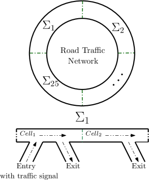
Figure 1. Model of a road traffic network in a circular highway composed of 25 identical links, each link has two cell.

Now, in order to apply the compositionality result, we introduce subsystems $\Sigma_{i}$, $\forall i\in[1;25]$. Each subsystems $\Sigma_{i}$ represents the dynamic of one link of the entire highway, where each link contains $2$ cells, one entry, and two exits, as schematically illustrated in Figure 1. The subsystems $\Sigma_{i}$ is described by

$$\Sigma_{i}:\left\{\begin{array}[]{rl}\mathbf{x}_{i}(k+1)&=A_{i}\mathbf{x}_{i}(k)+D_{i}w_{i}(k)+B_{i\mathsf{p}_{i}(k)},\\ \mathbf{y}_{1i}(k)&=\mathbf{x}_{i}(k),\\ \mathbf{y}_{2i}(k)&=C_{2i}\mathbf{x}_{i}(k),\end{array}\right.$$

$$A_{i}\!\!=\!\!\begin{bmatrix}\!0.9\!-\!\!\frac{\tau v}{d}\!\!&0\\ \frac{\tau v}{d}\!\!&0.65\!-\!\!\frac{\tau v}{d}\!\end{bmatrix}\!\!,D_{i}\!\!=\!\!\begin{bmatrix}\frac{\tau v}{d}\\ 0\\ \end{bmatrix}\!\!,B_{i1}\!\!=\!\!\begin{bmatrix}0\\ 0\\ \end{bmatrix}\!\!,\!B_{i2}\!\!=\!\!\begin{bmatrix}12\\ 0\\ \end{bmatrix}\!\!,C_{2i}\!\!=\!\!\begin{bmatrix}0\\ 1\end{bmatrix}^{T}\!\!\!\!\!\!,$$

and the set of modes is $P_{i}=\{1,2\}$, $\forall i\in[1;25]$. Clearly, $\Sigma=\mathcal{I}(\Sigma_{1},\ldots,\Sigma_{25})$, where the elements of the coupling matrix $M$ are $\{M\}_{(i+1)i}=\{M\}_{1(25)}=1$, $\forall i\in[1;25]$, and all other elements are identically zero.

Note that, for any $i\in[1;25]$, conditions (16) and (17) are satisfied with $S_{ip_{i}}(x_{i},\hat{x}_{i})\!=\!{(x_{i}-\hat{x}_{i})^{T}Z_{ip_{i}}(x_{i}-\hat{x}_{i})}$, $Z_{ip_{i}}=I_{2}$, $\underline{\alpha}_{ip_{i}}(s)=s^{2}$, $\kappa_{ip_{i}}=0.98$, $Q_{ip}^{11}=0.3527$, $Q_{ip}^{12}=Q_{ip}^{21}=0.0937$, $Q_{ip}^{22}=-0.6785$ $\forall p_{i}\in P_{i}$. Moreover, since $S_{ip_{i}}=S_{ip^{\prime}_{i}},\forall p,p^{\prime}\in P$, and according to Remarks 16 and 17, function $\mathcal{V}_{i}((x_{i},p_{i},l_{i}),(\hat{x}_{i},p_{i},l_{i}))=\!S_{i}(x_{i},\hat{x}_{i})$ is an augmented-storage function from $\hat{T}_{i}(\hat{\Sigma}_{i})$, constructed as in Definition 11, to $T_{i}(\Sigma_{i})$, defined in Definition 2. Now, by choosing $\mu_{i}=1,\forall i\in[1;25]$ and finite internal input sets $\hat{W}_{i}$ of $\hat{T}_{i}(\hat{\Sigma}_{i})$ in such a way that $\prod_{i=1}^{25}\!\hat{W}_{i}\!\!=\!\!M\prod_{i\!=\!1}^{25}\!\hat{X}_{i}$, condition (13) and (14) are satisfied. Therefore, applying Theorem 8, function $\tilde{\mathcal{S}}((x,p,l),(\hat{x},p,l))\!=\!\!\sum_{i=1}^{25}\!\mathcal{V}_{i}((x_{i},p_{i},l_{i}),(\hat{x}_{i},p_{i},l_{i}))$ is an alternating simulation function from $\hat{\mathcal{I}}(\hat{T}_{1}(\hat{\Sigma}_{1}),\ldots,\hat{T}_{25}(\hat{\Sigma}_{25}))$ to $\mathcal{I}(T_{1}(\Sigma_{1}),\ldots,T_{25}(\Sigma_{25}))$.

Let us now design a controller for $\Sigma$ via symbolic models $\hat{T}_{i}(\hat{\Sigma}_{i})$ such that controllers maintain the density of traffic lower than $30$ vehicles per cell (safety constraint), and to allow only 2 consecutive red lights for each traffic signal (fairness constraint). The former constraint implies that each vehicle can keep a $30$-meter safe distance from the one directly in front. The latter constraint is a way to avoid the trivial solution (always red) of the safety constraint and ensures fairness between modes 1 and 2. The idea here is to design local controllers for symbolic models $\hat{T}_{i}(\hat{\Sigma}_{i})$, and then refine them to the ones for concrete switched subsystems $\Sigma_{i}$. To do so, the local controllers are designed while assuming that the other subsystems meet their specifications. This approach, called assume-guarantee reasoning [HSR98], allows for the compositional synthesis of controllers.

Note that the direct computation of the symbolic model for the original $50$-dimensional system $\Sigma$ is not possible monolithically. To the best of our knowledge, there does not exist any software toolbox for constructing symbolic models of systems with this number of state variables. On the other hand, we are able to construct the interconnected symbolic model and controllers for the $50$-dimensional system $\Sigma$ by applying the proposed compositionality method here. We leverage software tool SCOTS [RZ16] for constructing symbolic models and controllers for $\Sigma_{i}$ compositionally with the state quantization parameter $\eta_{i}=0.03$ and the computation times are amounted to $10.2s$ and $0.014s$, respectively. Figure 2 shows the applied modes of sample subsystem $\Sigma_{i}$. Moreover, the closed-loop state trajectories of $\Sigma$, consisting of $50$ cells, are illustrated in Figure 3.

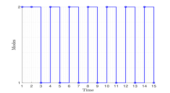
Figure 2. Applied modes of sample subsystem $\Sigma_{i}$.

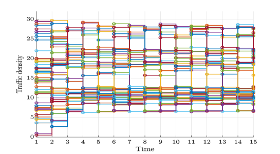
Figure 3. Closed-loop state trajectories of system $\Sigma$ consisting of $50$ cells.

6.2. Fully Connected Network

In this example, we apply our results to an interconnected switched systems $\Sigma$ composed of $N\geq 2$ linear switched subsystems $\Sigma_{i},i\in[1;N],$ admitting multiple $\delta$-P storage functions and supply rates. In this respect, we choose the dynamics’ parameters such that neither condition $\eqref{e:SFC11}$ nor $\eqref{e:SFC22}$ holds with common $\delta$-P storage functions and supply rates for all subsystems. In particular, as all subsystems are affine switched systems, we choose their the dynamics’ parameters such that the solution of the linear matrix inequality $\eqref{lmi}$ with common $Z_{i}$ and $Q_{i}$ (i.e. $Z_{ip_{i}}\!=\!Z_{ip^{\prime}_{i}}$ and $Q_{ip_{i}}\!=\!Q_{ip^{\prime}_{i}}$, $\forall p,p^{\prime}\!\in\!P,i\!\in\![1;N]$) is infeasible. Hence, non of the subsystems admits a common $\delta$-P storage function and supply rate. The dynamic of the interconnected switched system $\Sigma$ has the set of modes $P\!\!=\!\!\{1,2\}^{N},N\!\!\in\!\!\mathbb{N}_{\geq 2}$, and it is given by

$$\Sigma:\left\{\begin{array}[]{rl}\mathbf{x}(k+1)&=A_{\mathsf{p}(k)}\mathbf{x}(k)+B_{\mathsf{p}(k)},\\ \mathbf{y}(k)&=\mathbf{x}(k).\end{array}\right.$$

The vector $B_{p}\in\mathbb{R}^{n}$, where $n=2N$, is defined as $\{B\}_{i1}=B_{p_{i}}$ such that $B_{p_{i}}=[-0.9;0.5]$ if $p_{i}=1$, and $B_{p_{i}}=[0.9;-0.2]$ if $p_{i}=2$, $\forall i,j\in[1;N],i\neq j$. The elements of the matrix $A_{p}\in\mathbb{R}^{n\times n}$ are as follows:

$$\{A\}_{ij}\!=\!\begin{bmatrix}0.015\!\!\!&0\\ 0\!\!\!&0.015\\ \end{bmatrix}\!\!,\{A\}_{ii}\!\!=\!\!A_{p_{i}}\!\!=\!\!\left\{\begin{array}[]{lr}\!\!\!\!\begin{bmatrix}0.05\!\!\quad&0\\ 0.9&0.03\\ \end{bmatrix}\quad\!\!\text{if}~{}p_{i}=1,\vspace{0.1cm}\\ \!\!\!\!\begin{bmatrix}0.02&-1.2\\ 0&0.05\\ \end{bmatrix}\quad\text{if}~{}p_{i}=2.\end{array}\right.$$

Now, by introducing $\Sigma_{i}$ described by

$$\Sigma_{i}:\left\{\begin{array}[]{rl}\mathbf{x}_{i}(k+1)&=A_{i\mathsf{p}_{i}(k)}\mathbf{x}_{i}(k)+\omega_{i}(k)+B_{i\mathsf{p}_{i}(k)},\\ \mathbf{y}_{i1}(k)&=\mathbf{x}_{i}(k),\\ \mathbf{y}_{i2}(k)&=\mathbf{x}_{i}(k),\end{array}\right.$$

$$A_{i1}\!\!=\!\!\begin{bmatrix}0.05\!\!\!\!\!\!\quad&0\\ 0.9&0.03\\ \end{bmatrix}\!\!,A_{i2}\!\!=\!\!\begin{bmatrix}0.02&-1.2\\ 0&0.05\\ \end{bmatrix}\!\!,B_{i1}\!\!=\!\!\begin{bmatrix}-0.9\\ 0.5\\ \end{bmatrix}\!\!,B_{i2}\!\!=\!\!\begin{bmatrix}0.9\\ -0.2\\ \end{bmatrix}\!\!,$$

and the set of modes is $P_{i}\!\!=\!\!\{1,2\}$, one can readily verify that $\Sigma\!=\!\mathcal{I}(\Sigma_{1},\ldots,\Sigma_{N})$, where the elements of the coupling matrix $M$ are $\{M\}_{ii}\!\!=\!\!0_{2}$ and $\{M\}_{i,j}\!\!=\!\!\{A\}_{i,j}$, $\forall i,j\in\!\![1;N],i\!\neq\!j$. Note that, for any $i\in[1;N]$, conditions (16) and (17) are satisfied with $S_{ip_{i}}(x_{i},\hat{x}_{i})\!=\!{(x_{i}-\hat{x}_{i})^{T}Z_{ip_{i}}(x_{i}-\hat{x}_{i})}$,

$$Z_{i1}=\begin{bmatrix}0.3030&0.0087\\ 0.0087&0.4938\end{bmatrix},Z_{i2}=\begin{bmatrix}0.4899&-0.0033\\ -0.0033&0.4291\end{bmatrix},$$

$Q_{i1}=10^{-3}L_{i1},\kappa_{i1}\!=\!0.7,\underline{\alpha}_{i1}(s)\!=\!0.3s^{2},,Q_{i2}=10^{-3}L_{i2},\kappa_{i2}\!=\!0.7,\underline{\alpha}_{i2}(s)\!=\!0.4s^{2}\!$, where

$$L_{i1}\!\!=\!\!\!\begin{bmatrix}2.7\!&\!0\!&\!-1\!&\!\!-3\!\\ 0\!&\!1\!&\!-3\!&\!\!0\!\\ -1\!&\!-3\!&\!-201.3\!&\!\!-17\!\\ -3\!&\!0\!&\!-1.7\!&\!\!270.8\!\end{bmatrix}\!\!\!,L_{i2}\!\!=\!\!\!\begin{bmatrix}\!\!\!\!\!2.9\!&\!0\!&\!-1.4\!&\!\!2.7\!\\ 0\!&\!1.6\!&\!2.7\!&\!\!0\!\\ -1.4\!&\!2.7\!&\!156\!&\!\!17.5\!\\ 2.7\!&\!0\!&\!17.5\!&\!\!-294\!\end{bmatrix}$$

Since Assumption 13 and $k_{d}\geq\epsilon\frac{\ln(\mu)}{\ln(1/\kappa_{p})}+1$ hold with $\mu=1.63$, $k_{d}=3$, $\epsilon=1.01$, one can easily find a matrix $\tilde{Q}$ such that $\forall q\in\{1,2\},\tilde{Q}-0.7^{\frac{-q}{\epsilon}}\sum_{p=1}^{2}Q_{p}\succeq 0$ by using semi-definite programming such that function $\mathcal{V}_{i}((x_{i},p_{i},l_{i}),(\hat{x}_{i},p_{i},l_{i}))={\sum_{i=1}^{N}S_{ip_{i}}(x_{i},\hat{x}_{i})}{\kappa^{{-l}/{\epsilon}}_{p_{i}}}$ is an augmented-storage function from $\hat{T}_{i}(\hat{\Sigma}_{i})$ to $T_{i}(\Sigma_{i})$. Choose an arbitrary $N$, then by choosing $\mu_{1}\!=\!\cdots\!=\!\mu_{N}=1$ and finite internal input sets $\hat{W}_{i}$ of $\hat{T}_{i}(\hat{\Sigma}_{i})$ in such a way that $\prod_{i=1}^{N}\hat{W}_{i}=M\prod_{i=1}^{N}\hat{X}_{i}$, condition (13) and (14) are satisfied. Hence, using Theorem 8, function $\tilde{\mathcal{S}}((x,p,l),(\hat{x},p,l))\!=\!\!\sum_{i=1}^{N}\!\mathcal{V}_{i}((x_{i},p_{i},l_{i}),(\hat{x}_{i},p_{i},l_{i}))$ is an alternating simulation function from $\hat{\mathcal{I}}(\hat{T}_{1}(\hat{\Sigma}_{1}),\ldots,\hat{T}_{N}(\hat{\Sigma}_{N}))$ to $\mathcal{I}(T_{1}(\Sigma_{1}),\ldots,T_{N}(\Sigma_{N}))$.

Given $N\geq 5$, $X_{i}=[0,1]$, and $\eta_{i}=0.1$, we observe that constructing the symbolic model for the original system $\Sigma$ is only possible compositionally even with this small range of state set and coarse quantization parameters. The computation time for constructing symbolic models of $\Sigma_{i}$ is amounted to $0.53s$, using tool SCOTS [RZ16] with the state quantization parameter $\eta_{i}=0.1$.

7. Conclusion

In this work, we proposed a compositional scheme for the construction of symbolic models of interconnected discrete-time switched systems. First, we used a notion of augmented-storage functions in order to construct compositionally an alternating simulation function that is used to quantify the error between the output behavior of the interconnected switched system and that of its abstraction. Furthermore, under some assumptions ensuring incremental passivity of each mode of switched subsystems, we showed how to construct symbolic models together with their corresponding augmented-storage functions of the concrete systems.

References

• [AMP16] M. Arcak, C. Meissen, and A. Packard. Networks of dissipative systems. SpringerBriefs in Electrical and Computer Engineering. Springer International Publishing, 2016.
• [BK08] Christel Baier and Joost-Pieter Katoen. Principles of Model Checking (Representation and Mind Series). The MIT Press, 2008.
• [CGG13] E. Le Corronc, A. Girard, and G. Goessler. Mode sequences as symbolic states in abstractions of incrementally stable switched systems. In Proceedings of 52nd IEEE Conference on Decision and Control, pages 3225–3230, 2013.
• [dWOK12] Carlos Canudas de Wit, Luis Leon Ojeda, and Alain Y. Kibangou. Graph constrained-ctm observer design for the grenoble south ring. In Proceedings of 13th IFAC Symposium on Control in Transportation Systems, pages 197–202, 2012.
• [GGM16] A. Girard, G. Gössler, and S. Mouelhi. Safety controller synthesis for incrementally stable switched systems using multiscale symbolic models. IEEE Transactions on Automatic Control, 61(6):1537–1549, 2016.
• [GP09] A. Girard and G. J. Pappas. Hierarchical control system design using approximate simulation. Automatica, 45(2):566 – 571, 2009.
• [GPT10] A. Girard, G. Pola, and P. Tabuada. Approximately bisimilar symbolic models for incrementally stable switched systems. IEEE Tranctions on Automatic Control, 55(1):116–126, 2010.
• [HAT17] O. Hussein, A. Ames, and P. Tabuada. Abstracting partially feedback linearizable systems compositionally. IEEE Control Systems Letters, 1(2):227–232, 2017.
• [HSR98] T. A. Henzinger, Q. Shaz, and S. K. Rajamani. You assume, we guarantee: Methodology and case studies. In Proceedings of International Conference on Computer Aided Verification, pages 440–451, 1998.
• [KAZ18] Eric S. Kim, Murat Arcak, and Majid Zamani. Constructing control system abstractions from modular components. In Proceedings of the 21st International Conference on Hybrid Systems: Computation and Control, pages 137–146, 2018.
• [Kea11] Michael Keating. The Simple Art of SoC Design. Springer-Verlag, 2011.
• [Lib03] Daniel Liberzon. Switching in Systems and Control. Birkhäuser Basel, 2003.
• [Lof04] J. Lofberg. Yalmip : a toolbox for modeling and optimization in matlab. In Proceedings of the International Conference on Robotics and Automation, pages 284–289, 2004.
• [MGW17] P. J. Meyer, A. Girard, and E. Witrant. Compositional abstraction and safety synthesis using overlapping symbolic models. IEEE Transactions on Automatic Control, 63(6):1835–1841, 2017.
• [Mor96] A. S. Morse. Supervisory control of families of linear set-point controllers - part i. exact matching. IEEE Transactions on Automatic Control, 41(10):1413–1431, 1996.
• [MPS95] O. Maler, A. Pnueli, and J. Sifakis. On the synthesis of discrete controllers for timed systems. In Proceedings of the 12th Symposium on Theoretical Aspects of Computer Science, pages 229–242, 1995.
• [MSSM18] K. Mallik, A-K Schmuck, S. Soudjani, and R. Majumdar. Compositional synthesis of finite state abstractions. IEEE Transactions on Automatic Control, 2018.
• [PPB16] G. Pola, P. Pepe, and M. D. Di Benedetto. Symbolic models for networks of control systems. IEEE Transactions on Automatic Control, 61(11):3663–3668, 2016.
• [PPB18] G. Pola, P. Pepe, and M. D. D. Benedetto. Decentralized supervisory control of networks of nonlinear control systems. IEEE Transactions on Automatic Control, 63(9):2803–2817, Sept 2018.
• [RZ16] Matthias Rungger and Majid Zamani. SCOTS: A tool for the synthesis of symbolic sontrollers. In Proceedings of the 19th International Conference on Hybrid Systems: Computation and Control, pages 99–104, 2016.
• [SG17] Adnane Saoud and Antoine Girard. Multirate symbolic models for incrementally stable switched systems. In Proceedings of 20th IFAC World Congress, pages 9278 – 9284, 2017.
• [SGZ18] A. Swikir, A. Girard, and M. Zamani. From dissipativity theory to compositional synthesis of symbolic models. In Proceedings of the 4th Indian Control Conference, pages 30–35, 2018.
• [SZ18] Abdalla Swikir and Majid Zamani. Compositional synthesis of finite abstractions for networks of systems: A small-gain approach. CoRR, abs/1805.06271, 2018.
• [Tab09] Paulo Tabuada. Verification and Control of Hybrid Systems: A Symbolic Approach. Springer Publishing Company, Incorporated, 1st edition, 2009.
• [TI08] Y. Tazaki and J. I. Imura. Bisimilar finite abstractions of interconnected systems. In Proceedings of the 11th International Conference on Hybrid Systems: Computation and Control, pages 514–527, 2008.
• [VCL07] L. Vu, D. Chatterjee, and D. Liberzon. Input-to-state stability of switched systems and switching adaptive control. Automatica, 43(4):639 – 646, 2007.
• [ZA17] M. Zamani and M. Arcak. Compositional abstraction for networks of control systems: A dissipativity approach. IEEE Transactions on Control of Network Systems, 5(3):1003–1015, 2017.
• [ZMEM+14] M. Zamani, P. Mohajerin Esfahani, R. Majumdar, A. Abate, and J. Lygeros. Symbolic control of stochastic systems via approximately bisimilar finite abstractions. IEEE Transactions on Automatic Control, 59(12):3135–3150, 2014.