Constructing High Precision Knowledge Bases
with Subjective and Factual Attributes

Abstract

Knowledge bases (KBs) are the backbone of many ubiquitous applications and are thus required to exhibit high precision. However, for KBs that store subjective attributes of entities, e.g., whether a movie is kid friendly, simply estimating precision is complicated by the inherent ambiguity in measuring subjective phenomena. In this work, we develop a method for constructing KBs with tunable precision–i.e., KBs that can be made to operate at a specific false positive rate, despite storing both difficult-to-evaluate subjective attributes and more traditional factual attributes. The key to our approach is probabilistically modeling user consensus with respect to each entity-attribute pair, rather than modeling each pair as either True or False. Uncertainty in the model is explicitly represented and used to control the KB’s precision. We propose three neural networks for fitting the consensus model and evaluate each one on data from Google Maps–a large KB of locations and their subjective and factual attributes. The results demonstrate that our learned models are well-calibrated and thus can successfully be used to control the KB’s precision. Moreover, when constrained to maintain 95% precision, the best consensus model matches the F-score of a baseline that models each entity-attribute pair as a binary variable and does not support tunable precision. When unconstrained, our model dominates the same baseline by 12% F-score. Finally, we perform an empirical analysis of attribute-attribute correlations and show that leveraging them effectively contributes to reduced uncertainty and better performance in attribute prediction.

1 Introduction

Structured knowledge repositories–known as knowledge bases (KBs)–are the backbone of many high-impact applications and services. For example: the Netflix movie recommendation engine relies on a KB of user-movie-rating triples, Google Maps is built atop a KB of geographic points of interest and PubMed offers a handful of tools that operate on its citation KB of biomedical research. Wikipedia is both a KB (with respect to infoboxes) and a service in and of itself and has even inspired and facilitated the creation of additional KBs like YAGO and DBPedia [32, 18].

In KBs that support real-world decision making, maintaining high precision is often critical. As an example, consider organizing a lunch meeting and issuing a KB query for cafes that are good for groups. In the KB’s response, it is far better to omit a few true positives (i.e., cafes that are good for groups) than it is to return any false positives (i.e., cafes that are not good for groups), because choosing to visit a false positive could lead to a highly unproductive meeting. The importance of high precision can be even more pronounced for queries about factual data–like a query for restaurants that are wheelchair accessible–where false positives may be inaccessible by the user issuing the query. Since most KBs are built using noisy automated methods, special consideration must be paid. Previous work echos this concern: in addition to employing trained automated components for data collection and prediction of missing values, systems that build KBs often turn to humans–largely considered to be more precise than the automated methods–for validation, writing inference rules, identifying relevant features, labeling data and even responding to queries [6, 5, 23, 13, 21, 24].

Supporting control over the precision of KB query-responses requires that each element of a response have an associated probability of being True, or score, by which it can be filtered. For KBs that store subjective data (in addition to factual data), supporting such control is evasive because of the inherent ambiguity in measuring subjective phenomena. As a concrete example, consider a query for romantic locations in Paris, France, and deciding whether or not to include the Pont des Arts–a.k.a., The Love Lock Bridge–in the response set. The bridge is neither definitively romantic nor unromantic making it unclear how best to compute the probability of it being romantic, and thus complicating the decision of whether or not it should be filtered out.

This work develops a method for constructing a KB of entities and their attributes that offers tunable precision–that is, the KB can be set to run with a particular false positive rate, even when it stores subjective attributes. To begin, we define the yes rate of an entity-attribute pair to be the fraction of users who believe that the entity exhibits the attribute, as the number of surveyed users goes to infinity. If ground-truth yes rates were available, the attributes of an entity could be determined by thresholding the corresponding yes rates. For example, when queried for locations that are romantic a KB might only return locations with yes rates higher than 0.9. However, ground-truth yes rates are never fully observed and attempts to survey enough users for empirical yes rate estimation for every entity-attribute pair are easily stymied by the scale of most KBs.

Therefore, we propose a hybrid (i.e., human-machine) approach to constructing KBs, which at its heart employs a probabilistic model for yes rate estimation. Our approach begins with crowdsourcing: we serve users questions of the form: “does entity $e$ exhibit attribute $a$?” and we receive yes votes and no votes in response (users may also abstain). We use the votes to bootstrap training of a probabilistic yes rate model for each entity-attribute pair. Uncertainty in each model is explicitly represented via a distinct prior distribution. The priors allow for quantifiable confidence when many votes are available and, in the more common case, quantifiable uncertainty when votes are scarce. Representing uncertainty is a crucial component of our approach because it is used to control the precision of the KB. When the KB is queried, entity-attribute pairs are only included in the response if the KB is sufficiently confident that their corresponding yes rate exceeds the threshold. As long as the learned models are well-calibrated, this approach can be used to control the KB’s false positive rate. The procedure can even be used with respect to factual attributes, where we expect yes rates to be close to 0 or 1 and where representing uncertainty helps make the KB robust to noise from crowdsourcing [31].

We study the KB that supports Google Maps. This KB stores real-world landmarks–called locations–and their subjective and factual attributes. Since the number of location-attribute pairs in Google Maps is large, fitting yes rate models using the votes alone renders most of the models highly uncertain. To mitigate uncertainty, we leverage side information that accompanies each location–like natural language text extracted from the location’s homepage–during learning. Intuitively, the side information is likely to be indicative of the location’s attributes. For example, finding the phrase “wine list” on a restaurant’s homepage may constitute strong evidence that the restaurant exhibits the attribute, serves alcohol. To further reduce model uncertainty, we also promote information sharing across attributes. This is beneficial when attributes are related. For example, a location that has many yes votes for the attribute romantic is unlikely to receive many yes votes for the attribute kid friendly. Both the side information and shared information can be used to address the cold start problem–i.e., predicting the attributes of a location with no observed votes. This is critical for large KBs and for KBs with ever-expanding lists of entities and attributes, like Google Maps, in which cold starting is common.

We present three neural networks for estimating the yes rate of each location-attribute pair. Each network uses side information and is trained using a different style of information sharing across attributes. We evaluate the three networks on their ability to accurately represent uncertainty and predict attributes of the locations in Google Maps. When constrained to operate with 95% precision, our best model improves on the precision of an unconstrained baseline by 6% and matches the baseline’s F-score. This also amounts to a 5% increase in F-score over a neural baseline that uses multi-task learning–a common paradigm for information sharing–and that is subject to the same precision constraint (i.e., 95%). When unconstrained, our best model dominates both the empirical and neural baselines by 12% and 17% F-score, respectively. Additionally, our results reveal that some styles of information sharing lead to improved F-score by bolstering model confidence while others do not. This observation suggests that information sharing can be detrimental when performed between two attributes, one of which is data rich and the other is data poor. Finally, we demonstrate that our learned models are well-calibrated via Q-Q plots. While we study the location-attribute setting, our yes rate modeling framework can be applied in many instances of hybrid KB construction that rely on collecting categorical observations via crowdsourcing.

2 Locations, Attributes and Votes

We study the problem of constructing a knowledge base (KB) of locations and their attributes. The term location refers to a real-world landmark (e.g., a restaurant, monument, museum, business, park, etc.) and the term attribute refers to a characteristic of a landmark. Constructing the KB roughly refers to determining, for each location-attribute pair, whether the location exhibits the attribute. For example, the KB should store whether Starbucks at 1912 Pike Pl, Seattle is a local favorite. The KB stores subjective attributes (like local favorite) and factual attributes (like has free wifi). A subset of the attributes can be found in Table 1. In this work, we focus on the KB underlying Google Maps, which includes more than 50 million locations and more than 70 attributes.

Factual	Subjective
CASH_ONLY	BUSTLING
WHEELCHAIR_ACCESSIBLE	GOOD_VIEW
ACCEPTS_RESERVATIONS	COZY
HAS_HIGH_CHAIRS	KID_FRIENDLY
SERVES_FOOD_LATE	QUICK_VISIT

Table 1: A sample of factual and subjective attributes.

For each location, the KB has access to associated structured and unstructured meta-data known as side information. The unstructured side information for a location is comprised of text extracted from that location’s homepage and from other relevant web pages. The structured side information includes tags for that location that come from a proprietary ontology. Both the structured and unstructured side information are available as natural language text.

Crowdsourcing is used to gather yes votes and no votes for the location-attribute pairs. Specifically, users who have recently visited a particular location are served yes-or-no questions regarding the attributes of that location. Users may supply a yes vote, a no vote or an abstention in response. Despite the continuous deployment of these questions, in comparison to the number of location-attribute pairs, the number of votes is small: there are ~2.65 $\times$ $10^{8}$ location-attribute pairs, only ~13% of which have at least 1 associated vote, and, of those pairs, ~50% have only 1 vote. The votes are neither evenly distributed among locations or attributes nor are they guaranteed to be unanimous (i.e., many pairs receive both yes and no votes). See Figure 1 for a sketch of the number of yes and no votes collected for a subset of the attributes.

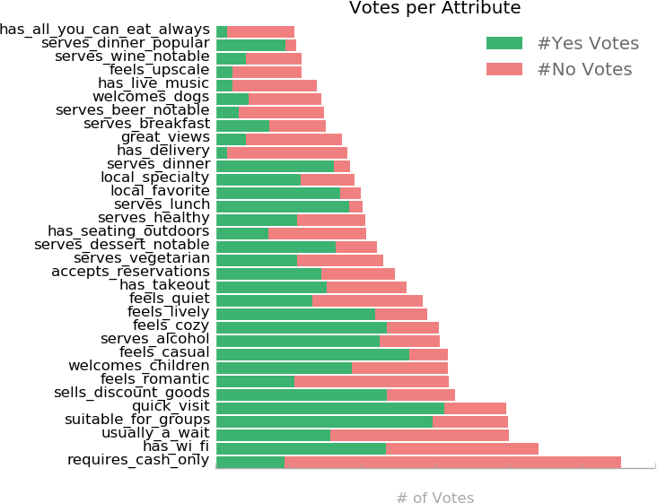
Figure 1: Yes and no votes for a subset of attributes. Precise vote counts have been omitted to respect data sensitivity.

3 The Observation Model

In constructing the KB, it is tempting to assume that each location-attribute pair is either True or False. However, this assumption does not hold for many pairs, especially those that include a subjective attribute. Therefore, we model the consensus among users with respect to each pair. In this section, we formalize this notion of consensus via a generative model of the observed votes.

3.1 Location-attribute Yes Rate

We assume that each location-attribute pair has a latent yes rate. The yes rate represents the fraction of users who agree that the location exhibits the attribute, i.e., it is a measure of consensus. Formally, for location $l$ and attribute $a$ let $0\leq\theta_{la}\leq 1.0$ be the yes rate for the pair. We model each vote for the pair $(l,a)$ as a sample from a pair-specific binomial distribution. The success parameter of this distribution is equal to the pair’s latent yes rate. Therefore,

$$Y_{la}\sim B(k,\theta_{la})$$

where $B(\cdot,\cdot)$ is the binomial distribution, $\theta_{la}$ is the yes rate and $Y_{la}$ is the number of yes votes out of $k$ total votes for the pair $(l,a)$.

3.2 Representing Uncertainty

Ideally, there would be enough votes to reliably estimate the yes rate for each location-attribute pair. However, the KB contains hundreds of millions of pairs, most of which have no corresponding votes. Therefore, we explicitly represent uncertainty in every pair’s yes rate through a pair-specific prior distribution. Specifically, each $\theta_{la}$ is modeled as a beta distributed random variable:

$$\theta_{la}\sim Beta(\mu_{la}\tau_{la},\tau_{la}(1-\mu_{la})).$$

Here, $\mu_{la}$ is the expected yes rate for the pair $(l,a)$–that is, $\mu_{la}$ represents the fraction of yes votes as the total votes goes to infinity:

$$\mu_{la}=\mathbb{E}\left[\frac{Y_{la}}{Y_{la}+N_{la}}\right]$$

where, $Y_{la}$ and $N_{la}$ are the number of yes and no votes for the pair $(l,a)$, respectively. $\tau_{la}$ is the prior distribution’s precision: in a sense, $\tau_{la}$ captures certainty in the true yes rate being close to $\mu_{la}$. This choice in representation precisely defines KB construction: estimate both $\mu_{la}$ and $\tau_{la}$ for each location-attribute pair.

There are a number of advantages to this hierarchical beta-binomial model for the observed votes. Most important for high precision KBs is that the model facilitates closed-form computation of its confidence in each estimated expected yes rate (further discussion appears in Section 7). As long as the model is well-calibrated, this allows the KB maintainer to control the false positive rate by filtering results by model confidence. Specifically, consider a query, $q$, for which the optimal result set includes all location-attribute pairs that satisfy $\theta_{la}>\mu_{min}$. To guarantee a false positive rate that is less than $\delta$ in expectation, for $q$, the KB maintainer can: gather all pairs where $\mu_{la}>\mu_{min}$ and filter out all pairs for which the KB has confidence less than $1-\delta$.

The structure of our model has other practical advantages, too. First, the prior beta distribution makes yes rate estimation more robust when only a few (or zero) votes are observed for a pair. Another practical advantage is that our model structure facilitates efficient updates: because of conjugacy, after observing additional votes for some location-attribute pair, it is possible to update the model’s estimates for the corresponding $\mu$ and $\tau$ efficiently. This is particularly valuable because the KB’s size makes fitting the model very expensive and because new votes are observed frequently.

4 Attribute Relatedness

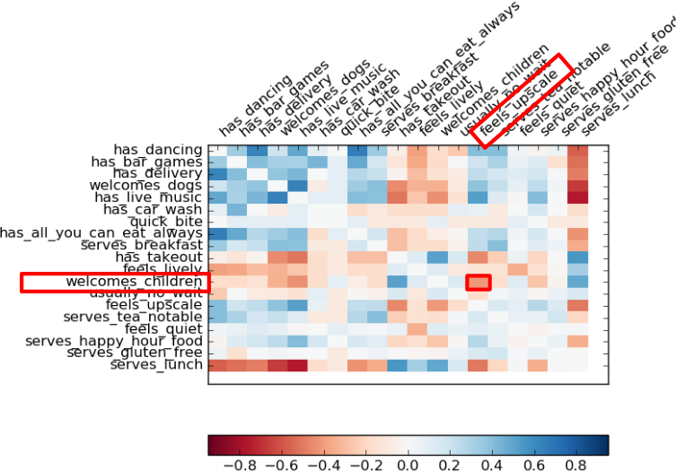
(a) Attribute pairs that generally exhibit negative relatedness.

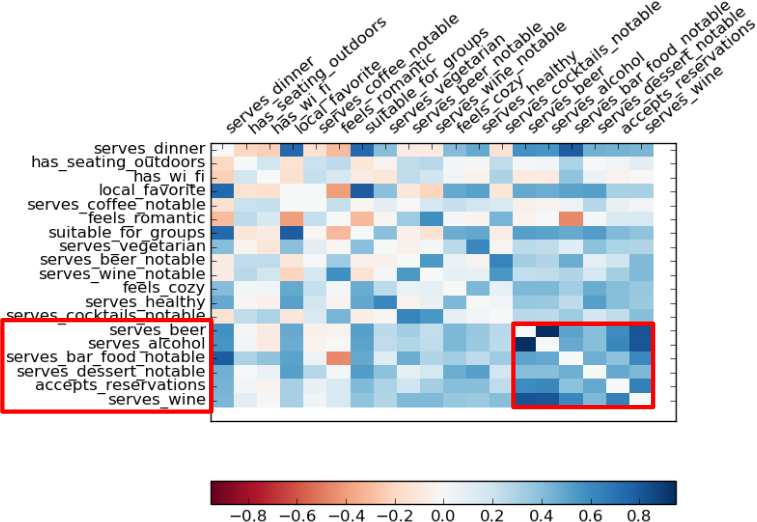
(b) Attribute pairs that generally exhibit positive relatedness.

Figure 2: Submatrices of the relatedness matrix. welcomes children and feels upscale are negatively related; serves beer, serves alcohol, serves bar food notable, serves dessert notable, accepts reservation and serves wine are all positively related.

The parameters of the observation model (Section 3) can be learned independently for each location-attribute pair. But, intuitively, many of the attributes are closely related to one another. For example, a location that has takeout probably does not feel upscale. Were attributes correlated with one another, jointly learning parameters across attributes would yield more accurate and confident models.

We present a qualitative analysis that highlights strong correlations between various attribute pairs. For each attribute-attribute pair, we count the number of locations for which both attributes agree–i.e., both have majority yes votes or both have majority no votes–and the number of locations for which the attributes disagree–i.e., one attribute has majority yes votes while the other has majority no votes. If there are an equal number of yes and no votes for a particular location-attribute pair, the attribute neither agrees nor disagrees with any other attribute (for that location). We construct a relatedness matrix of dimension $|A|\times|A|$, where $|A|$ is the number of attributes. Each cell in the matrix is computed by:

$$r_{ij}=\frac{\sum_{l\in L}[\mathrm{\emph{agree}}_{ij}]-[\mathrm{\emph{disagree}}_{ij}]}{|L|+b}$$

where $L$ is the set of all locations and $b$ is a bias term.

Figure 2 shows two quadrants of the relatedness matrix with rows and columns sorted by increasing sum-total relatedness and diagonal set to zero. The relationships depicted generally match intuition about the attributes that are positively and negatively related. However, not all pairs respect intuition, largely due to vote scarcity. For example, the attribute has car wash has very few votes and exhibits scores that may misrepresent its relatedness to other attributes. Regardless of the noise, the relatedness matrix suggests that learning from attribute-attribute correlations is useful.

5 Learning Model Parameters

In this section we propose three neural network architectures for estimating the parameters of the observation model (Section 3). Each architecture is designed to leverage information sharing across attributes differently.

5.1 Multi-task Baseline

The multi-task learning baseline architecture (ML), models each vote-generating distribution (i.e., $\mu_{la}$ and $\tau_{la}$) as follows:

$$\mu_{la} =\sigma\left(f_{\mu_{a}}^{(ml)}(e_{l})\right)$$

$$\tau_{la} =\log\left[1+\exp{\left(f_{\tau_{a}}^{(ml)}(e_{l})\right)}\right]$$

where $e_{l}$ is an embedded representation of location $l$, $f_{\mu_{a}}^{(ml)}(\cdot)$ and $f_{\tau_{a}}^{(ml)}(\cdot)$ are learnable, attribute-specific functions of the location embedding and $\sigma(\cdot)$ is the softmax function. $f_{\mu_{a}}^{(ml)}(\cdot)$ and $f_{\tau_{a}}^{(ml)}(\cdot)$ are trained to facilitate estimation of $\mu$ and $\tau$, respectively. The superscript $ml$ denotes that these functions are part of the ML baseline architecture. Notice that the architecture ensures that both $\mu$ and $\tau$ take values in appropriate domains.

The location embedding and the functions $f_{\mu_{a}}^{(ml)}(\cdot)$ and $f_{\tau_{a}}^{(ml)}(\cdot)$ are trained by maximizing the marginal likelihood, or evidence. That is, the training objective is to maximize the likelihood of the observed votes under the beta-binomial observation model. Because the beta distribution is conjugate to the binomial, it is possible to compute the evidence exactly. Letting $\alpha=\mu_{la}\tau_{la}$ and $\beta=\tau_{la}(1-\mu_{la})$, the evidence corresponding to the pair $(l,a)$ is:

$$\mathcal{L}_{la}(Y_{la};k,\mu_{la},\tau_{la})=\binom{k}{Y_{la}}\frac{1}{Z(\alpha,\beta)} \cdot Z(Y_{la}+\alpha,k-Y_{la}+\beta)$$

where $Z(\alpha,\beta)=\frac{\Gamma(\alpha)\Gamma(\beta)}{\Gamma(\alpha+\beta)}$ is the normalizer of the beta distribution.

The ML model uses multi-task learning, a standard technique for sharing information across related tasks [8]. In practice, the location embedding is updated with gradients computed with respect to each attribute. Intuitively, each embedding captures the salient features of the corresponding location.

5.2 Alien Vote Architecture

One shortcoming of the ML architecture is that information is shared indirectly via gradients. Our second architecture shares information more directly. In particular, this architecture leverages alien votes, where the alien votes for a pair $(l,a)$ are all votes for the attributes of $l$ excluding $a$. Formally, for a pair $(l,a)$, the alien votes are:

$$V_{l\bar{a}}=\{(l^{\prime},a^{\prime}):l^{\prime}=l,a^{\prime}\neq a\}.$$

Direct access to alien votes makes it easier to learn relationships like: a restaurant that has many yes votes for the attribute romantic is unlikely to be kid friendly.

We introduce the following alien vote architecture (AV):

$$\mu_{la} =\sigma\left(f_{\mu_{a}}^{(av)}(e_{l}\oplus g(V_{l\bar{a}}))\right)$$

$$\tau_{la} =\log\left[1+\exp{\left(f_{\tau_{a}}^{(av)}(e_{l}\oplus g(V_{l\bar{a}}))\right)}\right]$$

where the $\oplus$ operator denotes vector concatenation. In this architecture, the alien votes for a pair $(l,a)$ are transformed using a learned function $g(\cdot)$ and concatenated with the location embedding. The concatenation is then used to compute $\mu_{la}$ and $\tau_{la}$, facilitating direct learning of attribute-attribute correlations.

5.3 Independent AV Architecture

For multi-task learning to be effective, the same features must be useful for each task. Since some attributes are unrelated (Section 4), we introduce an independent alien vote (IAV) architecture that does not employ multi-task learning. Unlike the other architectures, the IAV architecture uses a separate network per attribute:

$$\mu_{la} =\sigma\left(f_{\mu_{a}}^{(iav)}(e_{la}^{+})\right)$$

$$\tau_{la} =\log\left[1+\exp{\left(f_{\tau_{a}}^{(iav)}(e_{la}^{+})\right)}\right]$$

where $e_{la}^{+}$ is a location embedding that is computed, in part, from the alien votes $V_{l\bar{a}}$. Thus, the IAV model still uses attribute-attribute correlations learned from the alien votes.

Under the IAV architecture, attributes with many votes enjoy exclusive access to the location embeddings and do not suffer from spurious gradients computed with respect to unrelated attributes. On the other hand, attributes with few votes cannot leverage the salient location features learned through multi-tasking.

6 Implementation

Each architecture is implemented as a feed-forward neural network. The networks use side information–and optionally alien votes–to estimate the expected yes rate (and associated uncertainty) of each location-attribute pair, including the pairs with no observed votes.

6.1 ML Baseline

The input to the ML architecture is the side information $x_{l}$ for a specific location $l$ (Section 2). We represent each token in the side information by a 285-dimensional embedding. These tokens are combined by summing their embeddings and computing the element-wise square root. This 285-dimensional embedding is passed through 5 fully-connected layers, each with 500 ReLU activation units. The resulting representation of the side information is the location embedding, $e_{l}$.

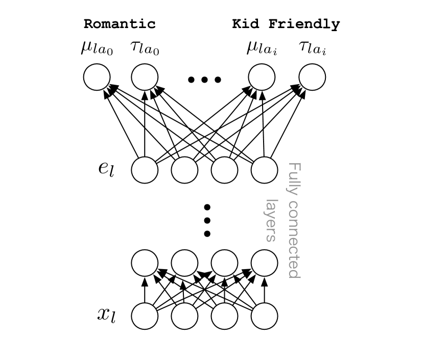
(a) Location Embedding.

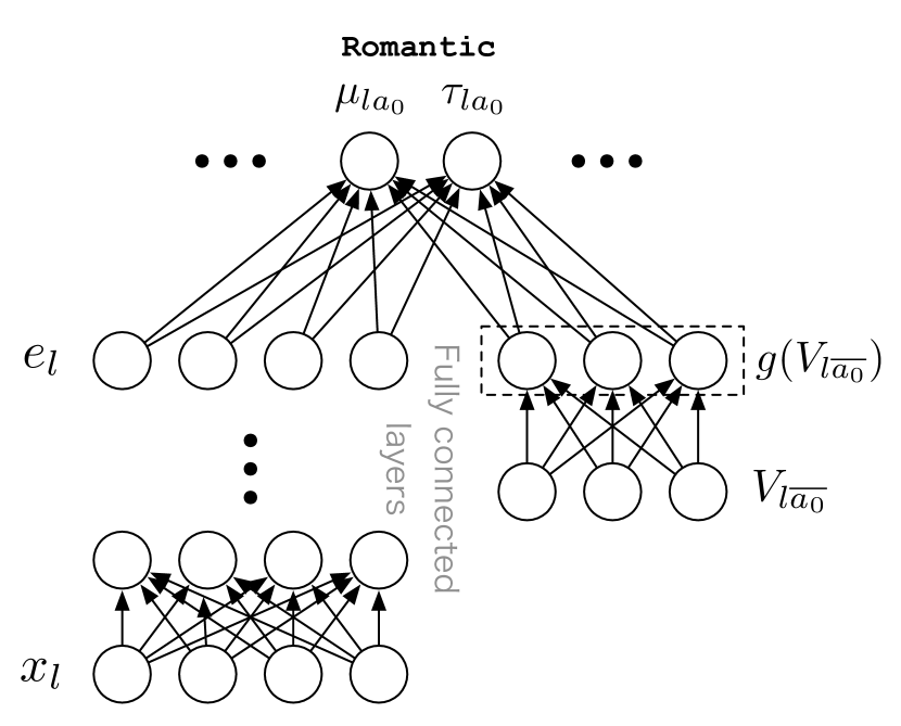
(b) Alien Votes.

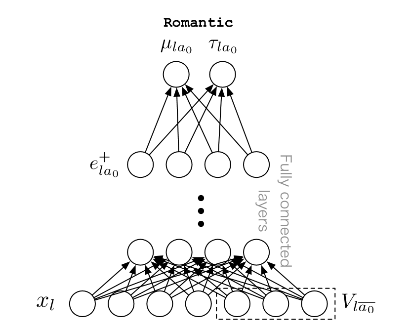
(c) Independent Alien Votes.

Figure 3: Three architectures that are trained to estimate parameters of the prior distributions of location-attribute pairs. Architectures 3(a) and 3(b) transform side information, $x_{l}$, into a location embedding, $e_{l}$, which can be transformed to estimate the parameters of each attribute for location $l$. Architecture 3(b) concatenates the same location embedding, $e_{l}$, with the transformed alien votes for each attribute, $V_{l\bar{a}}$, before estimating the corresponding parameters. In architecture 3(c), $x_{l}$ and the $V_{l\bar{a}}$ are transformed into an augmented embedding, $e_{la}^{+}$. Architecture 3(c) is duplicated for each attribute. In all architectures, the functions $f_{\mu_{a}}(\cdot)$ and $f_{\tau_{a}}(\cdot)$ correspond to the transformation of the location embedding into $\mu_{la}$ and $\tau_{la}$ respectively.

The location embedding, $e_{l}$, is used to estimate $\mu_{la}$ and $\tau_{la}$ for each attribute. Each attribute $a$ has two parallel sets of layers, one corresponding to $f_{\mu_{a}}^{(ml)}(\cdot)$ and the other corresponding to $f_{\tau_{a}}^{(ml)}(\cdot)$. The location embedding layer is fully connected to both.

To implement multi-task learning (and achieve additional regularization [4]) in each training mini-batch, all gradients computed with respect to $\mu_{la}$ are back-propagated through $f_{\mu_{a}}^{(ml)}(\cdot)$ and the location embedding; all gradients computed with respect to $\tau_{la}$ are back-propagated through $f_{\tau_{a}}^{(ml)}(\cdot)$ and also the location embedding. A visual representation of the network can be found in Figure 3(a).

6.2 AV Architecture

The implementation of the AV architecture builds on the baseline. In the AV architecture, the alien votes, $V_{l\bar{a}}$, represented as a dense vector, are passed through a single fully-connected layer (i.e., the function $g(\cdot)$ in Section 5.2) and then concatenated with the location embedding. While the alien votes may yield greater predictive power, they also result in an increase in model parameters and training time. The resulting architecture is depicted in Figure 3(b).

6.3 IAV Model

To implement the IAV architecture, we train a separate network for each attribute (Figure 3(c)). In each network, the alien votes are concatenated with the input rather than the location embedding. The IAV architecture has more parameters than the AV architecture but also avoids issues stemming from the multi-task learning.

7 Experimental Setup

Since the ground-truth yes rate of each location-attribute pair is not observed, we cannot evaluate a learned model using the residual between estimated and the ground-truth yes rates. Therefore, we evaluate the trained models via two other methods. First, we compute their F-scores in attribute prediction with respect to a set of gold labels (for a subset of locations and their subjective and factual attributes). Second, we measure model calibration.

7.1 Model-based Attribute Predictor

The primary responsibility of the KB is to retrieve all locations that exhibit a queried attribute. In doing so, recall that it is crucial for the result set to have very few false positives (while maintaining as high recall as possible). To accomplish this goal, for each query, the KB maintainer sets a yes rate threshold, $\mu_{min}$, and a false positive rate, $\delta$. For each query, we use a predictor $s(\cdot,\cdot)$ to build the result set, where the predictor is defined as:

$$s(l,a)=\begin{cases}1&\text{if }Pr(R\geq\mu_{min};\mu_{la},\tau_{la})\geq 1-\delta\\ 0&\text{if }Pr(R\leq 1-\mu_{min};\mu_{la},\tau_{la})\geq 1-\delta\\ \text{No Prediction}&\text{otherwise}\end{cases}$$

and where $R$ represents a yes rate. In words, if, with probability at least $1-\delta$, the yes rate for a pair $(l,a)$ is greater than $\mu_{min}$, then the predictor outputs a 1; if, with probability at least $1-\delta$, the yes rate for a pair $(l,a)$ is less than $1-\mu_{min}$, then the predictor outputs a 0; otherwise there is insufficient confidence in the yes rate being greater than $\mu_{min}$ or less than $1-\mu_{min}$ so the predictor outputs “No Prediction”. The probabilities used by the predictor are computed via the cumulative distribution function (CDF) of a beta distribution, for example:

$$Pr(R\geq\mu_{min};\mu_{la},\tau_{la}) =\int_{\mu_{min}}^{1}Pr(\theta_{la}|\mu_{la},\tau_{la})d\theta_{la}$$

$$=1-\int_{0}^{\mu_{min}}Pr(\theta_{la}|\mu_{la},\tau_{la})d\theta_{la}.$$

In our experiments, we use the implementation of the CDF of the beta distribution included in Tensorflow [2] and we set the yes rate and uncertainty thresholds as follows: $\mu_{min}=0.66$ and $1-\delta=0.95$.

7.2 Data and Evaluation Metrics

We evaluate our models on a dataset that includes the real-world locations and attributes in Google Maps. The yes and no votes are collected by soliciting real users for their opinions about the attributes of the locations they have visited. We collect a separate set of gold labels, $\mathcal{G}$, from vetted workers. The gold label for the pair $(l,a)$ is a judgment $g_{la}\in\{0,1\}$, computed by a majority vote among three vetted workers regarding whether location $l$ exhibits attribute $a$. For any location-attribute pair there can be at most 1 corresponding gold label.

We measure the F-score of the attribute predictor $s(\cdot,\cdot)$ with respect to $\mathcal{G}$. The F-score of the predictor is the harmonic mean between the predictor’s precision and recall. We report the F-score of the predictor with respect to both the prior and posterior parameters (Section 3). Because of our model’s structure, the posterior parameters can be computed in closed form:

$$Pr(\theta_{la}|Y_{la},k) =\frac{Pr(Y_{la}|k,\theta_{la})Pr(\theta_{la}|\mu_{la},\tau_{la})}{\int_{0}^{1}Pr(Y_{la}|k,\hat{\theta}_{la})Pr(\hat{\theta}_{la}|\mu_{la},\tau_{la})d\hat{\theta}_{la}}$$

$$=Beta(Y_{la}+\mu_{la}\tau_{la},k-Y_{la}+\tau_{la}(1-\mu_{la}))$$

where $Z(\cdot,\cdot)$ denotes the beta function (Section 5.1). Note that computing the posterior from the prior is efficient because it only requires incrementing the parameters of a beta distribution. Also, note that increasing $\tau$, which is related to model confidence, has a similar effect on the posterior as observing additional votes.

While the F-score of the predictor is a good indication of model quality, it may be imprecise. To see why, consider the location-attribute pairs that have a ground-truth yes rate of 0.66, i.e., $\mathcal{P}_{0.66}=\{(l,a):\theta_{la}=0.66\}$. In expectation, 66% of votes for these pairs will be yes votes and 34% will be no votes (thus reflecting the True yes rate). For each pair in $\mathcal{P}_{0.66}$ the probability that the gold label will be “0” is equal to the probability of at least 2 out of 3 vetted workers labeling that pair with a “0”:

$$Pr(g_{la}=0|(l,a)\in\mathcal{P}_{0.66}) =\binom{3}{2}\cdot 0.66\cdot 0.34^{2}+0.34^{3}=0.268.$$

If a model correctly estimates a yes rate of 0.66 for each pair $(l,a)\in\mathcal{P}_{0.66}$ with high confidence, then for each such pair the predictor $s(\cdot,\cdot)$ will output “1”. Since the vetted workers only label ~75% of these pairs with “1”, the maximum attainable precision is ~75% even though the model is perfect.

Despite this limitation, we argue that our evaluation scheme sufficiently captures model quality. First, for attributes with yes rates close to 0 or 1 (e.g., most factual attributes) the effect of this imprecision is minor. Second, the gold labels in $\mathcal{G}$ correspond to pairs for which there is high worker agreement (e.g., for most pairs, worker votes are unanimous). Assuming that workers are reliable, the number of location-attribute pairs with little consensus in the gold set will be small. We also note that for the subjective attributes, our evaluation scheme produces a conservative estimate of model quality, which, we argue, is better than a non-conservative estimate given the importance of mitigating false positives.

We supplement the F-score evaluation with model calibration measurements. These measurements directly evaluate the model’s yes rate estimates rather than the discrete output of the predictor.

8 Experiments

For training, we use the Adagrad [11] optimizer with learning rate of 0.1 and a batch size of 256. We compare the 3 architectures (Section 5) with two additional empirical baselines. We also analyze how different information sharing paradigms affect attribute prediction. Finally, we provide Q-Q plots showing that our trained models are well-calibrated.

8.1 Attribute Prediction

We compare the models learned via the 3 architectures. For the AV and IAV architectures, we test 3 alien vote representations (Section 5.2): 1. raw: the raw counts of both yes and no votes, 2. maj: the majority vote (either yes or no), 3. prob: the expected value and 1 - the expected value of a beta distribution (with uniform prior) that is fit using the observed votes. We compare the models to two empirical baselines. One baseline (Empirical) predicts a “1” when the observed yes rate for a pair is greater than $\mu_{min}$. The second, more precise baseline (Empirical-P) only makes predictions for pairs with at least 3 observed votes. We also show the performance of the IAV raw model operating in “high-recall mode” (IAV-HR), meaning that a “1” is predicted when $\mu_{la}>0.66$ and no additional filtering (based on confidence) is performed.

	Prior			Posterior
Model	PRE	REC	F1	PRE	REC	F1
ML Baseline	0.98	0.40	0.57	0.97	0.52	0.67
AV raw	0.96	0.46	0.63	0.96	0.54	0.69
AV maj	0.95	0.42	0.58	0.95	0.52	0.68
AV prob	0.95	0.47	0.63	0.95	0.56	0.70
IAV raw	0.94	0.51	0.66	0.94	0.59	0.72
IAV maj	0.95	0.47	0.63	0.95	0.55	0.70
IAV prob	0.93	0.49	0.64	0.94	0.54	0.69
Empirical	—	—	—	0.88	0.61	0.72
Empirical-P	—	—	—	0.90	0.41	0.56
IAV-HR	0.88	0.77	0.82	0.89	0.80	0.84

Figure 4: Prior and posterior precision, recall and F-score of 3 baselines (ML and Empirical(-P)), 2 alien vote models (AV and IAV) and the IAV model in high-recall mode. The neural models outperform the empirical models and the alien vote models outperform the neural baseline.

Table 4 reveals a number of interesting model characteristics. First, all neural models achieve between 6%-9% better posterior precision (Section 7.2) than the Empirical baseline. The IAV raw model is even able to achieve comparable F-score to the empirical baseline even though it is constrained to maintain 95% precision. When this constraint is dropped (i.e., the IAV-HR model), the model dominates both the Empirical and Empirical-P baselines by 12% and 28% F-score, respectively. Note that the two baselines have no corresponding prior performance because they rely entirely on the observed votes (i.e., they do not use side information).

The AV and IAV models outperform the neural baseline (ML) in terms of F-score. This supports our hypothesis regarding the advantages of direct access to the alien votes during learning. Under the 5% false positive rate, the IAV model achieves the highest F-score of the neural models. This might stem from its increased number of parameters, but may also be the result of its information sharing mechanism (Section 5.3). We observe that the ML baseline has the highest precision, but generally exhibits comparatively lower recall. We hypothesize that the ML baseline is less confident than the other models resulting in fewer predictions made by $s(\cdot,\cdot)$. The raw and prob alien vote representations produce slightly better models than the maj representation, but no representation is dominant.

Finally, note that the precision of all neural models are close to 95%, showing that the KB’s precision can accurately controlled.

8.2 Information Sharing and AVs

	Prior			Posterior
Model	PRE	REC	F1	PRE	REC	F1
AV raw	0.96	0.49	0.65	0.96	0.59	0.73
Zeroed	0.97	0.37	0.53	0.97	0.52	0.68

Figure 5: F-score of the AV raw and Zeroed models. The Zeroed model has worse recall but high precision suggesting that alien votes help to increase model confidence.

We are interested in understanding why the alien vote models perform better than the ML baseline. To do so, we conduct the following experiment: first, we train the AV raw model; then, we create a Zeroed model from the trained AV raw model by artificially converting all input alien vote vectors to zero vectors at test time. Table 5 compares the performance of the Zeroed and AV raw models. While the two models have similar precision, the Zeroed model has worse recall. This is because the Zeroed model is, overall, less confident in its estimates (i.e., lower $\tau_{la}$). Lower confidence leads to fewer predictions made by $s(\cdot,\cdot)$ (i.e., a higher number of “No Prediction” outputs), which in turn leads to lower recall. We conclude that the AV model estimates yes rates effectively with side information alone and learns to use the alien votes to boost confidence.

Figure 6 shows histograms of $\tau_{la}$ estimated by the ML baseline and AV raw models. These histograms are evidence that the ML baseline tends to estimate lower values of $\tau_{la}$ than the AV model. This supports our hypothesis that the ML baseline’s relatively lower confidence is the cause of its lower F-score.

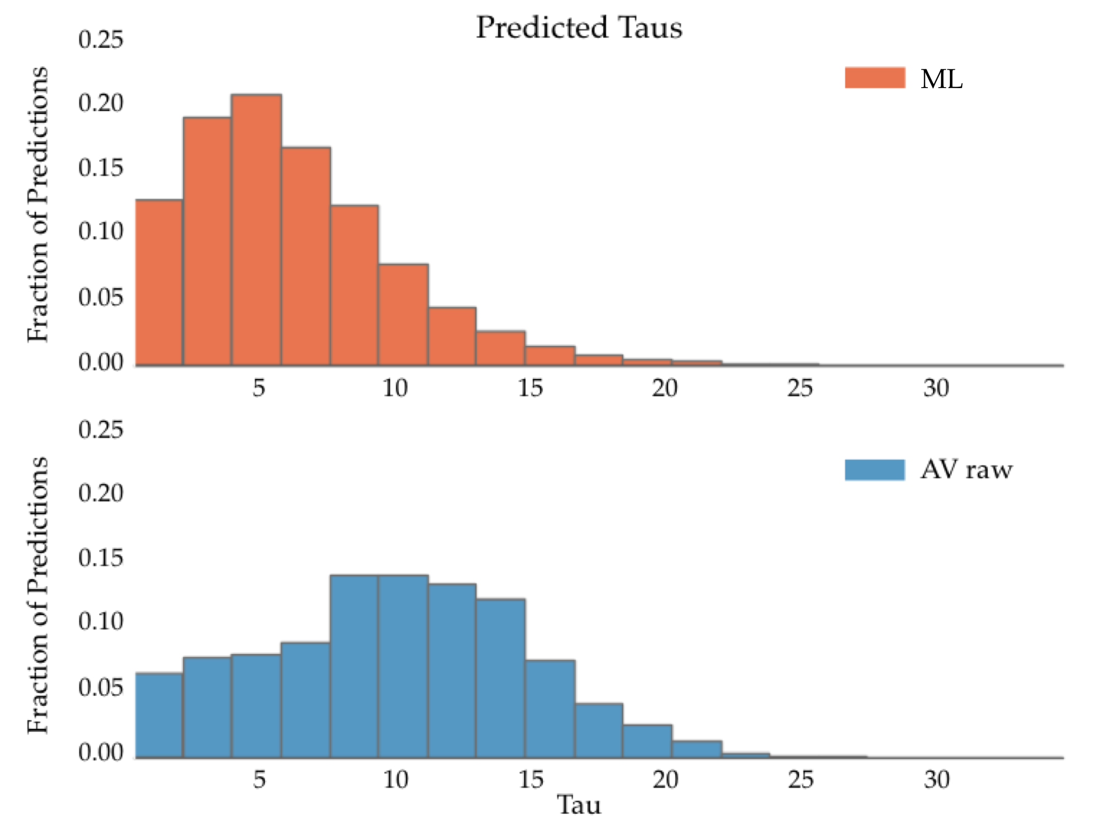
Figure 6: Histograms of estimated $\tau_{la}$ (model confidence) for all location-attribute pairs in the test set.

8.3 Model Calibration

For a more precise evaluation, we plot model calibration of the ML and AV raw models. To measure calibration, we first collect a test set of all location-attribute pairs that received $n$ total votes. Next, we select two integers, $Y$ and $N$–representing a number of yes and no votes respectively–such that $Y+N=n$. We use each model to compute $Pr(Y|k,\mu_{la})$, i.e., the probability of observing $Y$ yes votes and $N$ no votes, for each location-attribute pair in the test set. The locations are binned according to these probabilities.

We construct Q-Q plots showing the fraction of pairs in each bin for which the observed votes were exactly $Y$ yes votes and $N$ no votes (Figure 7). For a well-calibrated model, approximately $p$ (a fraction) of the items in the bin corresponding to the probability $p$ should be classified correctly (i.e., have exactly $Y$ yes and $N$ no votes). Since the predictions from both models closely track the line $y=x$ (Figure 7), we conclude that our models are well-calibrated. We build Q-Q plots with respect to 1 yes vote and 2 yes votes because these correspond to the first and second moments of the prior yes rate distribution, respectively. Q-Q plots corresponding to the other models reveal similar trends with respect to calibration; they are elided for brevity.

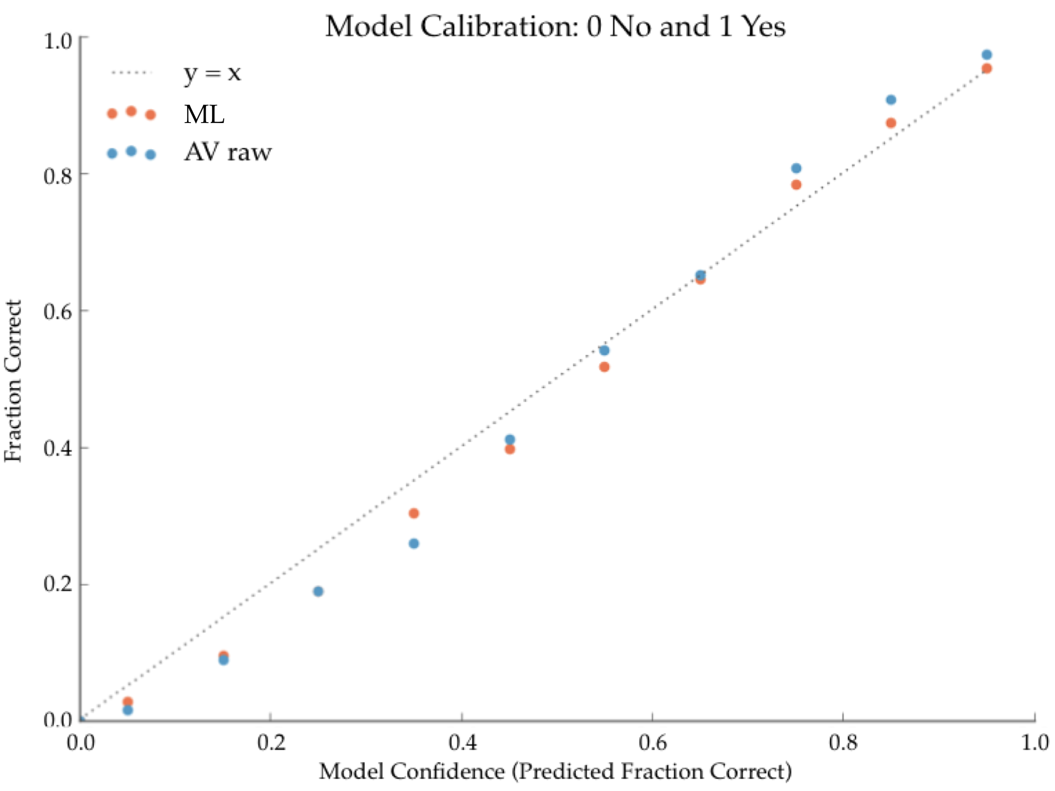
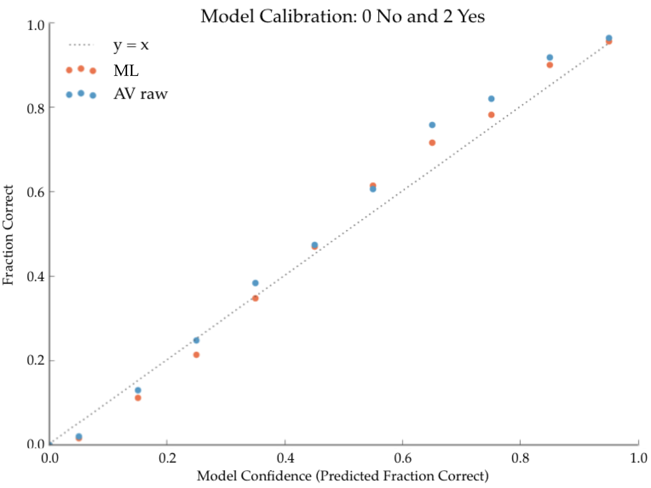
Figure 7: Calibration of the ML and AV raw models for location-attribute pairs that received one and two total votes.

9 Related Work

The literature on crowdsourcing for data collection and subsequent model training is vast. Most approaches collect multiple redundant labelings for a set of tasks from a handful of crowd workers and then infer the true task labels. Even in cases where the tasks are subjective, the true labels are considered to correspond to the majority opinion [22]. Many of these methods learn latent variable models of user expertise and task difficulty; the learned models can be used for inferring the task labels [27, 34]. Some work models both worker reputation and each item’s label as a real-valued random variable (in $[0,1]$) with a beta prior [10]. Like we do, other work develops beta-binomial models of the observed labels [7]. Unlike the prior art, we do not explicitly model the crowd workers. This is beneficial because it does not require collecting a minimum number of labels per worker and also protects worker anonymity. Whereas some previous work employs expectation-maximization [35], variational inference [20], Markov Chain Monte Carlo, or variants of belief propagation [17], we estimate parameters via back-propagation in neural networks. Some studies develop intelligent routing of tasks to workers based on task difficulty and user ability [17, 16]. In our work, questions are routed to geographically relevant users.

In this work, the model trained for attribute prediction can be characterized as a latent factors model. Previous work develops both probabilistic and non-probabilistic factorization models. Probabilistic matrix factorization techniques [30] pose generative models of the latent row and column representations and the observations. These models can be extended to incorporate side information as in our set up [26, 25, 19]. Much of the work on probabilistic matrix factorization models assumes that the observations are corrupted with Gaussian noise; this is not appropriate for our observed votes. More similar to our work are studies of Poisson factorization, which naturally models count data [14, 15]. While our work is not fully probabilistic, we do employ a generative model of the observations.

There are a number of methods for learning parameters of factorization models. For example, some methods leverage Bayesian Personalized Ranking [28, 29] while others utilize MCMC [19]. Many modern methods, like ours, perform learning via back-propagation in neural networks. These approaches are trained end-to-end and incorporate side information using various embedding techniques [33, 36, 3, 12]. Some work demonstrates the benefits of multi-task learning for neural matrix factorization [4].

The incorporation of alien votes (Section 5.2) is similar to the CoFactor model [19]. The work on CoFactor optimizes an extension of Gaussian matrix factorization and includes a column co-occurrence term. An analog to this co-occurrence term in our framework is captured by attribute relatedness (Section 4) and made directly available to our models via the alien votes. The AV architecture is loosely inspired by wide and deep architectures [9].

10 Conclusion

We study constructing a high precision KB of locations and their subjective and factual attributes. We probabilistically model the latent yes rate of each location-attribute pair, rather than modeling each pair as either True or False. Model confidence is explicitly represented and used to control the KB’s false positive rate. In experiments, we demonstrate that our models: 1) are well-calibrated and 2) that they outperform 1 neural and 2 empirical baselines. The experiments also reveal how different modes of information sharing across attributes affect performance. While our experiments are focused on the KB of locations and attributes that supports Google Maps, our proposed framework is useful for constructing KBs with tunable precision from unlabeled side information and noisy categorical observations collected via crowdsourcing.

References

- [1]
- Abadi et al. [2015] Martín Abadi et al. 2015. TensorFlow: Large-Scale Machine Learning on Heterogeneous Systems.
- Almahairi et al. [2015] A. Almahairi, K. Kastner, K. Cho, and A. Courville. 2015. Learning distributed representations from reviews for collaborative filtering. In Conference on Recommender Systems.
- Bansal et al. [2016] T. Bansal, D. Belanger, and A. McCallum. 2016. Ask the GRU: Multi-task Learning for Deep Text Recommendations. In Conference on Recommender Systems.
- Bennett et al. [2007] J. Bennett, S. Lanning, et al. 2007. The netflix prize. In Knowledge Discovery in Databases Cup and Workshop. New York, NY, USA.
- Carlson et al. [2010] A. Carlson et al. 2010. Toward an Architecture for Never-Ending Language Learning.. In Conference on Artificial Intelligence.
- Carpenter [2008] B. Carpenter. 2008. Multilevel bayesian models of categorical data annotation. Unpublished manuscript (2008).
- Caruana [1998] R. Caruana. 1998. Multitask learning. In Learning to learn.
- Cheng et al. [2016] H. Cheng et al. 2016. Wide & deep learning for recommender systems. In Workshop on Deep Learning for Recommender Systems.
- de Alfaro et al. [2015] L. de Alfaro, V. Polychronopoulos, and M. Shavlovsky. 2015. Reliable aggregation of boolean crowdsourced tasks. In Human Computation and Crowdsourcing.
- Duchi et al. [2011] J. Duchi, E. Hazan, and Y. Singer. 2011. Adaptive subgradient methods for online learning and stochastic optimization. Journal of Machine Learning Research (2011).
- Elkahky et al. [2015] A. M. Elkahky, Y. Song, and X. He. 2015. A multi-view deep learning approach for cross domain user modeling in recommendation systems. In International Conference on World Wide Web.
- Franklin et al. [2011] M. J. Franklin, D. Kossmann, T. Kraska, S. Ramesh, and R. Xin. 2011. CrowdDB: answering queries with crowdsourcing. In International Conference on Management of data.
- Gopalan et al. [2013] P. Gopalan, J. M. Hofman, and D. M. Blei. 2013. Scalable recommendation with poisson factorization. arXiv:1311.1704 (2013).
- Gopalan et al. [2014] P. K. Gopalan, L. Charlin, and D. Blei. 2014. Content-based recommendations with poisson factorization. In Neural Information Processing Systems.
- Ho et al. [2013] C.J. Ho, S. Jabbari, and J. W. Vaughan. 2013. Adaptive task assignment for crowdsourced classification. In International Conference on Machine Learning.
- Karger et al. [2011] D. R. Karger, S. Oh, and D. Shah. 2011. Iterative learning for reliable crowdsourcing systems. In Neural information processing systems.
- Lehmann et al. [2014] J. Lehmann et al. 2014. DBpedia - A Large-scale, Multilingual Knowledge Base Extracted from Wikipedia. Semantic Web Journal (2014).
- Liang et al. [2016] D. Liang, J. Altosaar, L. Charlin, and D. M. Blei. 2016. Factorization meets the item embedding: Regularizing matrix factorization with item co-occurrence. In Conference on Recommender Systems.
- Liu et al. [2012] Q. Liu, J. Peng, and A. T. Ihler. 2012. Variational inference for crowdsourcing. In Neural information processing systems.
- Marcus et al. [2011] A. Marcus, E. Wu, D. R. Karger, S. Madden, and R. C. Miller. 2011. Crowdsourced databases: Query processing with people. In Conference on Innovative Data Systems Research.
- Meng et al. [2017] R. Meng, H. Xin, L. Chen, and Y. Song. 2017. Subjective Knowledge Acquisition and Enrichment Powered By Crowdsourcing. arXiv:1705.05720 (2017).
- Niu et al. [2012] F. Niu, C. Zhang, C. Ré, and J. W. Shavlik. 2012. DeepDive: Web-scale Knowledge-base Construction using Statistical Learning and Inference. International Conference on Very Large Data search (2012).
- Parameswaran et al. [2012] A. G. Parameswaran, H. Park, H. Garcia-Molina, N. Polyzotis, and J. Widom. 2012. Deco: declarative crowdsourcing. In International conference on Information and knowledge management.
- Park et al. [2013] S. Park, Y. Kim, and S. Choi. 2013. Hierarchical Bayesian Matrix Factorization with Side Information.. In International Joint Conference on Artificial Intelligence.
- Porteous et al. [2010] I. Porteous, A. Asuncion, and M. Welling. 2010. Bayesian matrix factorization with side information and dirichlet process mixtures. In Conference on Artificial Intelligence.
- Raykar et al. [2010] V. C. Raykar, S. Yu, L. H. Zhao, G. H. Valadez, C. Florin, L. Bogoni, and L. Moy. 2010. Learning from crowds. Journal of Machine Learning Research (2010).
- Rendle et al. [2009] S. Rendle, C. Freudenthaler, Z. Gantner, and L. Schmidt-Thieme. 2009. BPR: Bayesian personalized ranking from implicit feedback. In Conference on uncertainty in artificial intelligence.
- Riedel et al. [2013] S. Riedel, L. Yao, A. McCallum, and B. M. Marlin. 2013. Relation extraction with matrix factorization and universal schemas. (2013).
- Salakhutdinov and Mnih [2007] R. Salakhutdinov and A Mnih. 2007. Probabilistic Matrix Factorization.. In Neural Information Processing Systems.
- Sheng et al. [2008] V. S. Sheng, F. Provost, and P. G. Ipeirotis. 2008. Get another label? improving data quality and data mining using multiple, noisy labelers. In International conference on Knowledge discovery and data mining.
- Suchanek et al. [2007] F. M. Suchanek, G. Kasneci, and G. Weikum. 2007. Yago: a core of semantic knowledge. In International conference on World Wide Web.
- Wang et al. [2015] H. Wang, N. Wang, and D. Yeung. 2015. Collaborative deep learning for recommender systems. In International Conference on Knowledge Discovery and Data Mining.
- Welinder et al. [2010] P. Welinder, S. Branson, P. Perona, and S. J. Belongie. 2010. The multidimensional wisdom of crowds. In Neural information processing systems.
- Whitehill et al. [2009] J. Whitehill, T. Wu, J. Bergsma, J. R. Movellan, and P. L. Ruvolo. 2009. Whose vote should count more: Optimal integration of labels from labelers of unknown expertise. In Neural information processing systems.
- Zheng et al. [2017] L. Zheng, V. Noroozi, and P. S. Yu. 2017. Joint deep modeling of users and items using reviews for recommendation. In International Conference on Web Search and Data Mining.