On Invariant Synthesis for Parametric Systems

Abstract

We study possibilities for automated invariant generation in parametric systems. We use (a refinement of) an algorithm for symbol elimination in theory extensions to devise a method for iteratively strengthening certain classes of safety properties to obtain invariants of the system. We identify conditions under which the method is correct and complete, and situations in which the method is guaranteed to terminate. We illustrate the ideas on various examples.

1 Introduction

In the verification of parametric systems it is important to show that a certain property holds for all states reachable from the initial state. One way to solve such problems is to identify an inductive invariant which entails the property to be proved. Finding suitable inductive invariants is non-trivial – the problem is undecidable in general; solutions have been proposed for specific cases, as discussed in what follows.

In [Kap06], Kapur proposes methods for invariant generation in theories such as Presburger arithmetic, real closed fields, and for polynomial equations and inequations with solutions in an algebraically closed field. The main idea is to use templates for the invariant (polynomials with undetermined coefficients), and solve constraints for all paths and initial values to determine the coefficients. A similar idea was used by Beyer et al. [BHMR07] for constraints in linear real or rational arithmetic; it is shown that if an invariant is expressible with a given template, then it will be computed. Symbol elimination has been used for interpolation and invariant generation in many papers. The methods proposed in [Kap06], where quantifier elimination or Gröbner bases computation are used for symbol elimination, are one class of examples. Quantifier elimination is also used by Dillig et al. in [DDLM13].

However, in some cases the investigated theories are complex (can be extensions or combinations of theories) and do not allow quantifier elimination. Methods for “symbol elimination” for such complex theories have been proposed, in many cases in relationship with interpolant computation. In [YM05] Yorsh et al. studied interpolation in combinations of theories; in [BGR14], Brutomesso et al. extended these results to non-convex theories. Interpolation in data structures by reduction was analyzed by Kapur, Majumdar and Zarba in [KMZ06]. Independently, in [Sof06, Sof08] Sofronie-Stokkermans analyzed possibilities of computing interpolants hierarchically, and in [Sof16, SS18] proposed a method of hierarchical symbol elimination which was used for interpolant computation; already [Sof13] mentions the possibility to infer constraints on parameters by hierarchical reasoning followed by quantifier elimination.

Symbol elimination can also be achieved using refinements of superposition. In [BGW94], Bachmair et al. mention the applicability of a form of hierarchical superposition to second-order quantifier elimination (i.e. to symbol elimination). This idea and possible links to interpolation are also mentioned in Ganzinger et al. [GSW04, GSW06]. In [KV09b], Kovács and Voronkov study inference systems and local derivations – in the context of interpolant generation – and symbol elimination in proofs in such systems. The ideas are concretized using the superposition calculus and its extension LASCA (ground linear rational arithmetic and uninterpreted functions). Applications to invariant generation (briefly mentioned in [KV09b]) are explored in detail in, among others, [KV09a, HKV10] – there Vampire is used to generate a large set of invariants using symbol elimination; only invariants not implied by the theory axioms or by other invariants are kept (some of these tasks are undecidable). In [GKR18], Gleiss et al. analyze functional and temporal properties of loops. For this, extended expressions (introduced in [KV09a]) are used; symbol elimination à la [KV09b] is used to synthesize invariants using quantification over iterations.

Various papers address the problem of strengthening a given formula to obtain an inductive invariant. In [BM08], Bradley proposes a goal-oriented invariant generation method for boolean/numeric transition systems, relying on finding counterexamples. Such methods were implemented in IC3 [Bra12]. For programs using only integers, Dillig et al. [DDLM13] use abductive reasoning based on quantifier elimination to obtain increasingly more precise approximations of inductive invariants (termination is not guaranteed). In [FK15], Falke and Kapur analyze various ways of strengthening the formulae; depending upon how strengthening is attempted, their procedure may also determine whether the original formula is not an invariant. Situations in which termination is guaranteed are identified. In [KBI⁺17], Karbyshev et al. propose a method to generate universal invariants in theories with the finite model property using diagram-based abstraction for invariant strengthening; Padon et al. [PIS⁺16] identify sufficient conditions for the decidability of inferring inductive invariants in a given language ${\cal L}$ and also present undecidability results. Invariant synthesis for array-based systems is studied by Ghilardi et al. in [GR10]; under local finiteness assumptions on the theory of elements and existence of well-quasi-orderings on configurations termination is guaranteed. In [ABG⁺14], Alberti et al. use lazy abstraction with interpolation-based refinement and discuss the applicability to invariant synthesis. A system for verifying safety properties that are “cubes” and invariant generation in array-based systems is described in [CGK⁺12]. In [GSV18], Gurfinkel et al. propose an algorithm extending IC3 to support quantifiers for inferring universal invariants in theories of arrays, combining quantified generalizations (to construct invariants) with quantifier instantiation (to detect convergence).

Our contribution. In this paper we continue the work on automated verification and synthesis in parametric systems started in [IJS08, Sof10, Sof13] by investigating possibilities for automated goal-oriented generation of inductive invariants. Our method starts with a universally quantified formula $\Psi$ and successively strengthens it, using a certain form of abductive reasoning based on symbol elimination. In case of termination we prove that we obtain a universal inductive invariant that entails $\Psi$, or the answer “no such invariant exists”. We identify situations in which the method terminates. Our main results are:

• We refine the symbol elimination method in theory extensions described in [Sof16, SS18] (Sect. 3). This helps us obtain shorter formulae during invariant synthesis.

• We propose a method for goal-oriented synthesis of universally quantified invariants which uses symbol elimination in theory extensions (Sect. 4).

• We identify conditions under which our invariant generation method is partially correct (Sect. 4) and situations in which the method terminates (Sect. 5.2).

• We further refine the method (Sect. 5) and provide examples in which the conditions we impose on the class of transition systems can be relaxed (Sect. 5.1).

The theories we analyze are extensions or combinations of theories and not required to have the finite model property – required e.g. in [KBI⁺17, PIS⁺16]. While we rely on methods similar up to a certain extent with the ones used in IC3 [BM08, Bra12], and the ones in [GR10, FK15, KBI⁺17] we here use possibilities of complete instantiation in local theory extensions and exploit (and refine) efficient methods for symbol elimination in theory extensions proposed in [Sof16, SS18].

Illustration. Consider for instance the program in Fig. 1, using subprograms ${\sf copy}(a,b)$, which copies the array $b$ into array $a$, and ${\sf add1}(a)$, which adds 1 to every element of array $a$.

  d1 = 1; d2 = 1;
  copy(a, b); i:= 0;
  while (nondet()) {
     a = add1(a);
     d1 = a[i]; d2 = a[i+1];
     i:= i + 1}

Figure 1: Program using subprograms and global function updates

The task is to prove that if $b$ is an array with its elements sorted in increasing order then the formula $\Psi:=d_{2}\geq d_{1}$ is an invariant of the program. $\Psi$ holds in the initial state; it is an inductive invariant of the while loop iff the formula

$\begin{array}[]{@{}l}\forall j(a^{\prime}[j]=a[j]+1)\wedge d^{\prime}_{1}=a^{\prime}[i]\wedge d^{\prime}_{2}=a^{\prime}[i+1]\wedge i^{\prime}=i+1\\ \wedge~{}d_{1}\leq d_{2}~{}\wedge~{}d^{\prime}_{1}>d^{\prime}_{2}\\ \end{array}$

is unsatisfiable. As this formula is satisfiable, $\Psi$ is not an inductive invariant.

We will show how to obtain the condition $\forall i(a[i]\leq a[i+1])$ which can be used to strengthen $\Psi:=d_{2}\geq d_{1}$ to the inductive invariant $(d_{2}\geq d_{1})\wedge\forall i(a[i]\leq a[i+1])$.

While we rely on methods similar to the ones used in [BM08, GR10, DDLM13, FK15, PIS⁺16, KBI⁺17, GSV18], there are several differences between our work and previous work.

The methods proposed in [Kap06, BM08, DDLM13, FK15] cannot be used to tackle examples like the one in Fig. 1: It is difficult to use templates in connection with additional function symbols; in addition, the methods of [BM08, DDLM13, FK15] can only handle numeric domains.

The theories we analyze are typically extensions or combinations of theories and not required to have the finite model property – which is required e.g. in [KBI⁺17, PIS⁺16].

The method proposed in [GSV18] does not come with soundness, completeness and termination guarantees. We here use possibilities of complete instantiation in local theory extensions and exploit (and refine) the methods for symbol elimination in theory extensions proposed in [Sof16, SS18].

The algorithm proposed in [GR10] for theories of arrays uses a non-deterministic function ChooseCover that returns a cover of a formula (as an approximation of the reachable states). If the theory of elements is locally finite it is proved that a universal formula $\Psi$ can be strengthened to a universal inductive invariant $I$ iff there exists a suitable ChooseCover function for which the algorithm returns an inductive invariant strengthening $\Psi$. In contrast, our algorithm is deterministic; we prove completeness under locality assumptions (holding if updates and properties are in the array property fragment); our termination results are established for classes of formulae for which only finitely many atomic formulae formed with a fixed number of variables can be generated using quantifier elimination. In addition our method allows us to choose the language for the candidate invariants (we can search for invariants not containing certain constants or function symbols).

The methods in [KV09b, KV09a, HKV10] use an approach different from ours: Whereas we start with a candidate invariant and successively strengthen it, there Vampire is used to generate a large set of invariants (by symbol elimination using versions of superposition combined with symbolic solving of recurrences); completeness/termination are not guaranteed, although the method works well in practice.

Structure of the paper. In Section 2 we present the verification problems we consider and the related reasoning problems, and present some results on local theory extensions. In Section 3 we present a method for symbol elimination in theory extensions introduced in [Sof16, SS18] and propose an improvement of the method. In Section 4 we present an approach to invariant synthesis, and identify conditions under which it is partially correct. Section 5 presents refinements and a termination result. In Section 6 we present the tools we used for our tests and the way we used them. Section 7 contains conclusions and plans for future work.

This paper is an extended version of [PSS19] containing full proofs and numerous examples.

Contents

1. 1 Introduction
2. 2 Preliminaries
   1. 2.1 Verification problems for parametric systems
   2. 2.2 Local Theory Extensions
3. 3 Quantifier elimination and symbol elimination
   1. 3.1 Symbol elimination in theory extensions
   2. 3.2 An improved algorithm
   3. 3.3 Example
4. 4 Goal-oriented invariant synthesis
   1. 4.1 Examples
5. 5 Refinements
   1. 5.1 Avoiding some of the conditions (A1)–(A5)
   2. 5.2 Termination
   3. 5.3 Termination vs. non-termination
6. 6 Tools for tests
7. 7 Conclusion
8. A Proof of Theorem 12

2 Preliminaries

We consider one-sorted or many-sorted signatures $\Pi=(\Sigma,{\sf Pred})$, resp. $\Pi=(S,\Sigma,{\sf Pred})$, where $S$ is a set of sorts, $\Sigma$ is a family of function symbols and ${\sf Pred}$ a family of predicate symbols. We assume known standard definitions from first-order logic (e.g. $\Pi$-structures, satisfiability, unsatisfiability, logical theories). We denote “falsum” with $\perp$. If $F$ and $G$ are formulae we write $F\models G$ (resp. $F\models_{\cal T}G$ – also written as ${\cal T}\cup F\models G$) to express the fact that every model of $F$ (resp. every model of $F$ which is also a model of ${\mathcal{T}}$) is a model of $G$. $F\models\perp$ means that $F$ is unsatisfiable; $F\models_{{\mathcal{T}}}\perp$ means that there is no model of ${\mathcal{T}}$ in which $F$ is true.

2.1 Verification problems for parametric systems

One of the application domains we consider is the verification of parametric systems. For modeling such systems we use transition constraint systems $T=(\Sigma,{\sf Init},{\sf Update})$ which specify: the function symbols $\Sigma$ (including a set $V$ of functions with arity 0 – the “variables” of the systems) whose values change over time; a formula ${\sf Init}$ specifying the properties of initial states; a formula ${\sf Update}$ with function symbols in $\Sigma\cup\Sigma^{\prime}$ (where $\Sigma^{\prime}$ consists of copies of symbols in $\Sigma$, such that if $f\in\Sigma$ then $f^{\prime}\in\Sigma^{\prime}$ is the updated function after the transition). Such descriptions can be obtained from system specifications (for an example cf. [FJS07]). With every specification of a system $S$, a background theory ${\cal T}_{S}$ – describing the data types used in the specification and their properties – is associated.

We can check in two steps whether a formula $\Psi$ is an inductive invariant of a transition constraint system $T{=}(\Sigma,{\sf Init},{\sf Update})$, by checking whether:

• ${\sf Init}\models_{\mathcal{T}_{S}}\Psi$; and

• $\Psi,{\sf Update}\models_{\mathcal{T}_{S}}\Psi^{\prime}$, where $\Psi^{\prime}$ results from $\Psi$ by replacing each $f\in\Sigma$ by $f^{\prime}$.

Checking whether a formula $\Psi$ is an invariant can thus be reduced to checking whether $\neg\Psi^{\prime}$ is satisfiable or not w.r.t. a theory ${\mathcal{T}}$. Even if $\Psi$ is a universally quantified formula (and thus $\neg\Psi^{\prime}$ is a ground formula) the theory ${\mathcal{T}}$ can be quite complex: it contains the axiomatization ${\mathcal{T}}_{S}$ of the datatypes used in the specification of the system, the formalization of the update rules, as well as the formula $\Psi$ itself. In [IJS08, Sof10, Sof13] we show that the theory ${\mathcal{T}}$ can often be expressed using a chain of extensions, typically including:

$${\mathcal{T}}_{0}~{}~{}\subseteq~{}~{}{\mathcal{T}}_{1}={\mathcal{T}}_{0}\cup\Psi~{}~{}\subseteq~{}~{}{\mathcal{T}}={\mathcal{T}}_{0}\cup\Psi\cup{\sf Update}$$

with the property that checking satisfiability of ground formulae w.r.t. ${\mathcal{T}}$ can be reduced to checking satisfiability w.r.t. ${\mathcal{T}}_{1}$ and ultimately to checking satisfiability w.r.t. ${\mathcal{T}}_{0}$. This is the case for instance when the theory extensions in the chain above are local (for definitions and further properties cf. Section 2.2).

Failure to prove (2) means that $\Psi$ is not an invariant or $\Psi$ is not inductive w.r.t. $T$. If $\Psi$ is not an inductive invariant, we can consider two orthogonal problems:

1. Determine constraints on parameters which guarantee that $\Psi$ is an invariant.

2. Determine a formula $I$ such that $\mathcal{T}_{S}\models I\rightarrow\Psi$ and $I$ is an inductive invariant.

Problem (a) was studied in [Sof10, Sof13]. In [Sof16, SS18] we proposed a method for hierarchical symbol elimination in theory extensions which allowed us to show that for local theory extensions the formulae obtained using this symbol elimination method are weakest constraints on parameters which guarantee that $\Psi$ is invariant. We present and improve this symbol elimination method in Section 3.

In this paper we address problem (b): in Section 6 we use symbol elimination for giving a complete method for goal-oriented invariant generation, for invariants containing symbols in a specified signature; we also identify some situations when termination is guaranteed. The safety property and invariants we consider are conjunctions of ground formulae and sets of (implicitly universally quantified) flat clauses of the form $\forall{\overline{i}}(C_{i}({\overline{c}},{\overline{i}})\vee C_{v}({\overline{c}},{\overline{i}},{\overline{f}}({\overline{i}})))$, where ${\overline{c}}$ are constants or constant parameters, ${\overline{f}}$ are functional parameters, $C_{i}$ is a clause containing constants and universally quantified variables, and $C_{v}$ a flat clause containing parameters, constants and universally quantified variables.

2.2 Local Theory Extensions

Let $\Pi_{0}=(\Sigma_{0},{\sf Pred})$ be a signature, and ${\cal T}_{0}$ be a “base” theory with signature $\Pi_{0}$. We consider extensions ${\mathcal{T}}:={\cal T}_{0}\cup{\mathcal{K}}$ of ${\cal T}_{0}$ with new function symbols $\Sigma$ (extension functions) whose properties are axiomatized using a set ${\mathcal{K}}$ of clauses in the extended signature $\Pi=(\Sigma_{0}\cup\Sigma,{\sf Pred})$, which contain function symbols in $\Sigma$. If $G$ is a finite set of ground $\Pi^{C}$-clauses and ${\mathcal{K}}$ a set of $\Pi$-clauses, we will denote by ${\sf st}({\cal K},G)$ (resp. ${\sf est}({\cal K},G)$) the set of all ground terms (resp. extension ground terms, i.e. terms starting with a function in $\Sigma$) which occur in $G$ or ${\cal K}$. If $T$ is a set of ground terms in the signature $\Pi^{C}$, we denote by ${\mathcal{K}}[T]$ the set of all instances of ${\mathcal{K}}$ in which the terms starting with a function symbol in $\Sigma$ are in $T$. Let $\Psi$ be a map associating with every finite set $T$ of ground terms a finite set $\Psi(T)$ of ground terms. For any set $G$ of ground $\Pi^{C}$-clauses we write ${\mathcal{K}}[\Psi_{\cal K}(G)]$ for ${\mathcal{K}}[\Psi({\sf est}({\cal K},G))]$. We define:

${\sf(Loc}_{f}^{\Psi})$	For every finite set $G$ of ground clauses in $\Pi^{C}$ it holds that
	${\mathcal{T}}_{0}\cup{\cal K}\cup G\models\bot$ if and only if ${\mathcal{T}}_{0}\cup{\mathcal{K}}[\Psi_{\cal K}(G)]\cup G$ is unsatisfiable.

Extensions satisfying condition ${\sf(Loc}_{f}^{\Psi})$ are called $\Psi$-local [IJS08, IS10]. If $\Psi$ is the identity, i.e. ${\mathcal{K}}[\Psi_{\cal K}(G)]={\mathcal{K}}[G]$, we have a local theory extension [Sof05].

Remark: In [IJS08, IS10] we introduced and studied a notion of extended locality, in which the axioms in ${\mathcal{K}}$ are of the form $\forall{\overline{x}}(\phi({\overline{x}})\vee C)$, where $\phi$ is an arbitrary $\Sigma_{0}$-formula and $C$ a clause containing extension symbols and the set $G$ contains ground formulae of the form $\Psi\vee G_{e}$, where $\Psi$ is a $\Sigma_{0}$-sentence and $G_{e}$ a ground clause containing extension symbols. While most of the results in this paper can be lifted by replacing “locality” with “extended locality”, in this paper we only refer to locality for the sake of simplicity.

Hierarchical reasoning in local theory extensions.

For ($\Psi$)-local theory extensions hierarchical reasoning is possible. Below, we discuss the case of local theory extensions; similar results hold also for $\Psi$-local extensions. If ${\cal T}_{0}\cup{\cal K}$ is a local extension of ${\cal T}_{0}$ and $G$ is a set of ground $\Pi^{C}$-clauses, then ${\cal T}_{0}\cup{\cal K}\cup G$ is unsatisfiable iff ${\cal T}_{0}\cup{\cal K}[G]\cup G$ is unsatisfiable. We can reduce this last satisfiability test to a satisfiability test w.r.t. ${\cal T}_{0}$ as follows: We purify ${\cal K}[G]\cup G$ by

• introducing (bottom-up) new constants $c_{t}$ for subterms $t=f(g_{1},\dots,g_{n})$ with $f\in\Sigma$, $g_{i}$ ground $\Sigma_{0}\cup\Sigma_{c}$-terms,

• replacing the terms $t$ with the constants $c_{t}$, and

• adding the definitions $c_{t}\approx t$ to a set $D$.

We denote by ${\cal K}_{0}\cup G_{0}\cup D$ the set of formulae obtained this way. Then $G$ is satisfiable w.r.t. ${\cal T}_{0}\cup{\cal K}$ iff ${\cal K}_{0}\cup G_{0}\cup{\sf Con}_{0}$ is satisfiable w.r.t. ${\cal T}_{0}$, where

${\sf Con}_{0}=\{(c_{1}\approx d_{1}\wedge\dots\wedge c_{n}\approx d_{n})\rightarrow c\approx d\mid c\approx f(c_{1},\dots,c_{n}),d\approx f(d_{1},\dots,d_{n})\in D\}.$

Theorem 1 ([Sof05])

If ${\cal T}_{0}\subseteq{\cal T}_{0}\cup{\cal K}$ is a local extension and $G$ is a finite set of ground clauses, then we can reduce the problem of checking whether $G$ is satisfiable w.r.t. ${\cal T}_{0}\cup{\cal K}$ to checking the satisfiability w.r.t. ${\cal T}_{0}$ of the formula ${\cal K}_{0}\cup G_{0}\cup{\sf Con}_{0}$ constructed as explained above.

If ${\cal K}_{0}\cup G_{0}\cup{\sf Con}_{0}$ belongs to a decidable fragment of ${\cal T}_{0}$, we can use the decision procedure for this fragment to decide whether ${\cal T}_{0}\cup{\cal K}\cup G$ is unsatisfiable.

As the size of ${\cal K}_{0}{\cup}G_{0}{\cup}{\sf Con}_{0}$ is polynomial in the size of $G$ (for a given ${\cal K}$), locality allows us to express the complexity of the ground satisfiability problem w.r.t. ${\cal T}_{1}$ as a function of the complexity of the satisfiability of formulae w.r.t. ${\cal T}_{0}$.

Examples of local theory extensions.

($\Psi$-)Local extensions can be recognized by showing that certain partial models embed into total ones [IS10]. Especially well-behaved are the theory extensions with property $({\sf Comp}_{f})$, stating that partial models can be made total without changing the universe of the model. The link between embeddability and locality allowed us to identify many classes of local theory extensions:

Example 1 (Extensions with free/monotone functions [Sof05, IJS08])

The following types of extensions of a theory ${\mathcal{T}}_{0}$ are local:

1. Any extension of ${\mathcal{T}}_{0}$ with uninterpreted function symbols ($({\sf Comp}_{f})$ holds).

2. Any extension of a theory ${\cal T}_{0}$ for which $\leq$ is a partial order with functions monotone w.r.t. $\leq$ (condition $({\sf Comp}_{f})$ holds if all models of ${\mathcal{T}}_{0}$ are complete lattices w.r.t. $\leq$).

Example 2 (Extensions with definitions [JK11, IJS08])

Consider an extension of a theory ${\mathcal{T}}_{0}$ with a new function symbol $f$ defined by axioms of the form:

$~{}~{}~{}~{}~{}~{}~{}~{}{\sf Def}_{f}:=\{\forall{\overline{x}}(\phi_{i}({\overline{x}})\rightarrow F_{i}(f({\overline{x}}),{\overline{x}}))\mid i=1,\dots,m\}$

(definition by “case distinction”) where $\phi_{i}$ and $F_{i}$, $i=1,\dots,m$, are formulae over the signature of ${\mathcal{T}}_{0}$ such that the following hold:

• $\phi_{i}({\overline{x}})\wedge\phi_{j}({\overline{x}})\models_{{\cal T}_{0}}\perp$ for $i{\neq}j$ and

• ${\cal T}_{0}\models\forall{\overline{x}}(\phi_{i}({\overline{x}})\rightarrow\exists y(F_{i}(y,{\overline{x}})))$ for all $i\in\{1,\dots,m\}$.

Then the extension is local (and satisfies $({\sf Comp}_{f})$). Examples:

1. Any extension with a function $f$ defined by axioms of the form:

   $~{}~{}~{}~{}~{}~{}~{}~{}{\sf D}_{f}:=\{\forall{\overline{x}}(\phi_{i}({\overline{x}})\rightarrow f({\overline{x}})\approx t_{i})\mid i=1,\dots,n\}$

   where $\phi_{i}$ are formulae over the signature of ${\mathcal{T}}_{0}$ such that (a) holds.

2. Any extension of ${\mathcal{T}}_{0}\in\{{\sf LI}({\mathbb{Q}}),{\sf LI}({\mathbb{R}})\}$ with functions satisfying axioms:

   $~{}~{}~{}~{}~{}~{}~{}~{}{\sf Bound}_{f}:=\{\forall{\overline{x}}(\phi_{i}({\overline{x}})\rightarrow s_{i}\leq f({\overline{x}})\leq t_{i})\mid i=1,\dots,n\}$

   where $\phi_{i}$ are formulae over the signature of ${\mathcal{T}}_{0}$, $s_{i},t_{i}$ are ${\mathcal{T}}_{0}$-terms, condition (a) holds and $\models_{{\cal T}_{0}}\forall{\overline{x}}(\phi_{i}({\overline{x}})\rightarrow s_{i}\leq t_{i})$ [IJS08].

Example 3 (The array property fragment [BMS06, IJS08])

In [BMS06] a decidable fragment of the theory of arrays is studied, namely the array property fragment. Arrays are regarded as functions with arguments of index sort and values of element sort. The index theory ${\cal T}_{i}$ is Presburger arithmetic. The element theory is parametric (for many-dimensional arrays: the element theories are parametric). Array property formulae are formulae of the form $(\forall i)(\varphi_{I}(i)\rightarrow\varphi_{V}(i))$, where

• $\varphi_{I}$ (the index guard) is a positive Boolean combination of atoms of the form $t{\leq}u$ or $t{=}u$ where $t$, $u$ are either variables or ground terms of index sort;

• $\varphi_{V}$ (the value constraint) has the property that any universally quantified variable of index sort $i$ only occurs in a direct array read $a(x)$ in $\varphi_{V}$ and array reads may not be nested.

The array property fragment consists of all existentially-closed Boolean combinations of quantifier-free formulae and array property formulae. In [BMS06] it is shown that formulae in the array property fragment have complete instantiation. In [IJS08] we showed that this fragment satisfies a $\Psi$-locality condition.

3 Quantifier elimination and symbol elimination

We now present possibilities of symbol elimination in complex theories.

A theory ${\mathcal{T}}$ over signature $\Pi$ allows quantifier elimination if for every formula $\phi$ over $\Pi$ there exists a quantifier-free formula $\phi^{*}$ over $\Pi$ which is equivalent to $\phi$ modulo ${\mathcal{T}}$. Examples of theories which allow quantifier elimination are rational and real linear arithmetic (${\sf LI}({\mathbb{Q}})$, ${\sf LI}({\mathbb{R}})$), the theory of real closed fields, and the theory of absolutely-free data structures.

We first analyze possibilities of eliminating existential quantifiers (EQE) in combinations of disjoint theories.

Remark 2 (EQE in combinations of disjoint theories)

Let ${\cal T}_{1}$ and ${\cal T}_{2}$ be theories over disjoint signatures $\Pi_{1}$ resp. $\Pi_{2}$. Let ${\cal T}$ be the two-sorted combination of the theories ${\cal T}_{1}$ and ${\cal T}_{2}$, with signature $\Pi=(\{s_{1},s_{2}\},\Sigma_{1}\cup\Sigma_{2},{\sf Pred}_{1}\cup{\sf Pred}_{2})$, where every $n$-ary operation $f\in\Sigma_{i}$ has sort $s_{i}^{n}\rightarrow s_{i}$, and every $m$-ary predicate symbol $p\in{\sf Pred}_{i}$ has arity $s_{i}^{m}$. Assume that ${\cal T}_{1}$ and ${\cal T}_{2}$ allow elimination of existential quantifiers. Let $F(x,{\overline{y}})$ be a quantifier-free $\Pi$-formula. Then $\exists xF(x,{\overline{y}})$ is equivalent w.r.t. ${\cal T}$ with a quantifier-free $\Pi$-formula $G({\overline{y}})$.

Proof: We can eliminate the existential variable $x$ from $\exists xF(x,{\overline{y}})$ by first bringing $F$ to disjunctive normal form, $F(x,{\overline{y}})\equiv\bigvee_{i=1}^{n}D_{i}(x,{\overline{y}})$, where every conjunction $D_{i}$ can be written as a conjunction $(D_{i}^{1}\wedge D_{i}^{2})$, where $D_{i}^{j}$ contains only atoms over the signature $\Pi_{j}$, $j=1,2$. Then $\exists xF(x,{\overline{y}})\equiv\bigvee_{i=1}^{n}\exists x(D_{i}^{1}(x,{\overline{y}})\wedge D_{i}^{2}(x,{\overline{y}}))$. If the variable $x$ is of sort $s_{1}$, then for every $i$, $x$ does not occur in $D_{i}^{2}$ and $\exists x(D_{i}^{1}(x,{\overline{y}})\wedge D_{i}^{2}({\overline{y}}))\equiv\exists x(D_{i}^{1}(x,{\overline{y}}))\wedge D_{i}^{2}({\overline{y}})$; a method for quantifier elimination for ${\cal T}_{1}$ can be used for computing formulae ${\overline{D}}_{i}({\overline{y}})$ with $\exists x(D_{i}^{1}(x,{\overline{y}}))\equiv{\overline{D}}_{i}({\overline{y}})$; the case in which the sort of the variable $x$ is $s_{2}$ is similar. $\Box$

3.1 Symbol elimination in theory extensions

Let $\Pi_{0}=(\Sigma_{0},{\sf Pred})$. Let ${\cal T}_{0}$ be a $\Pi_{0}$-theory and $\Sigma_{P}$ be a set of parameters (function and constant symbols). Let $\Sigma$ be a signature such that $\Sigma\cap(\Sigma_{0}\cup\Sigma_{P})=\emptyset$. We consider the theory extension ${\mathcal{T}}_{0}\subseteq{\mathcal{T}}_{0}\cup{\mathcal{K}}$, where ${\cal K}$ is a set of clauses in the signature $\Pi=\Pi_{0}\cup\Sigma_{P}\cup\Sigma$ in which all variables occur also below functions in $\Sigma_{1}=\Sigma_{P}\cup\Sigma$. Consider the symbol elimination method in Algorithm 1 [Sof16, SS18].

Algorithm 1 Symbol elimination in theory extensions [Sof16, SS18]

Step 1

Let ${\mathcal{K}}_{0}\cup G_{0}\cup{\sf Con}_{0}$ be the set of $\Pi_{0}^{C}$-clauses obtained from ${\mathcal{K}}[T]\cup G$ after the purification step described in Theorem 1 (with set of extension symbols $\Sigma_{1}$).

Step 2

Let $G_{1}={\mathcal{K}}_{0}\cup G_{0}\cup{\sf Con}_{0}$. Among the constants in $G_{1}$, we identify

1. the constants $c_{f}$, $f\in\Sigma_{P}$, where $c_{f}$ is a constant parameter or $c_{f}$ is introduced by a definition $c_{f}\approx f(c_{1},\dots,c_{k})$ in the hierarchical reasoning method,

2. all constants ${\overline{c}_{p}}$ occurring as arguments of functions in $\Sigma_{P}$ in such definitions.

Let ${\overline{c}}$ be the remaining constants. We replace the constants in ${\overline{c}}$ with existentially quantified variables ${\overline{x}}$, i.e. instead of $G_{1}({\overline{c}_{p}},{\overline{c}_{f}},{\overline{c}})$ we consider the formula $\exists{\overline{x}}G_{1}({\overline{c}_{p}},{\overline{c}_{f}},{\overline{x}})$.

Step 3

Using a method for quantifier elimination in ${\mathcal{T}}_{0}$ we can construct a formula $\Gamma_{1}({\overline{c}_{p}},{\overline{c}_{f}})$ equivalent to $\exists{\overline{x}}G_{1}({\overline{c}_{p}},{\overline{c}_{f}},{\overline{x}})$ w.r.t. ${\mathcal{T}}_{0}$.

Step 4

Let $\Gamma_{2}({\overline{c}_{p}})$ be the formula obtained by replacing back in $\Gamma_{1}({\overline{c}_{p}},{\overline{c}_{f}})$ the constants $c_{f}$ introduced by definitions $c_{f}:=f(c_{1},\dots,c_{k})$ with the terms $f(c_{1},\dots,c_{k})$. We replace ${\overline{c}_{p}}$ with existentially quantified variables ${\overline{y}}$.

Step 5

Let $\forall{\overline{y}}\Gamma_{T}({\overline{y}})$ be $\forall{\overline{y}}\neg\Gamma_{2}({\overline{y}})$.

Theorem 3 ([Sof16, SS18])

Assume that ${\cal T}_{0}$ allows quantifier elimination. For every finite set of ground $\Pi^{C}$-clauses $G$, and every finite set $T$ of ground terms over the signature $\Pi^{C}$ with ${\sf est}(G)\subseteq T$, Steps 1–5 yield a universally quantified $\Pi_{0}\cup\Sigma_{P}$-formula $\forall{\overline{x}}\Gamma_{T}({\overline{x}})$ such that ${\cal T}_{0}\cup\forall{\overline{y}}\Gamma_{T}({\overline{y}})\cup{\cal K}\cup G$ is unsatisfiable.

Theorem 4 ([Sof16, SS18])

Assume that the theory extension ${\cal T}_{0}\subseteq{\cal T}_{0}\cup{\cal K}$ satisfies condition $({\sf Comp}_{f})$ and ${\mathcal{K}}$ is flat and linear and every variable occurs below an extension symbol. Let $G$ be a set of ground $\Pi^{C}$-clauses, and $\forall{\overline{y}}\Gamma_{G}({\overline{y}})$ be the formula obtained with Algorithm 1 for $T={\sf est}({\mathcal{K}},G)$. Then $\forall y\Gamma_{G}(y)$ is entailed by every universal formula $\Gamma$ with ${\cal T}_{0}\cup\Gamma\cup{\cal K}\cup G\models\perp$.

A similar result holds if $T$ is the set of instances obtained from instantiation in a chain of theory extensions ${\mathcal{T}}_{0}\subseteq{\mathcal{T}}_{0}\cup{\mathcal{K}}_{1}\subseteq\dots\subseteq{\mathcal{T}}_{0}\cup{\mathcal{K}}_{1}\cup\dots\cup{\mathcal{K}}_{n}$, all satisfying condition $({\sf Comp}_{f})$, where ${\mathcal{K}}_{1},\dots,{\mathcal{K}}_{n}$ are all flat and linear and every variable is guarded by an extension function [SS18].

Remark. Algorithm 1 can be tuned to eliminate constants $c$ in a set $C_{e}$ which might occur as arguments to parameters: All these constants, together with all constants $c_{f}$ introduced by definitions $c_{f}=f(c_{1},\dots,c_{n})$ with some $c_{i}\in C_{e}$, are replaced with variables at the end of Step 2 and are eliminated in Step 3.

3.2 An improved algorithm

Quantifier elimination usually has high complexity and leads to large formulae. Often, Algorithm 1 can be improved such that QE is applied to smaller formulae:

Theorem 5

Assume that ${\mathcal{K}}={\mathcal{K}}_{P}\cup{\mathcal{K}}_{1}$ such that ${\mathcal{K}}_{P}$ contains only symbols in $\Sigma_{0}\cup\Sigma_{P}$ and ${\mathcal{K}}_{1}$ is a set of $\Pi$-clauses such that

$${\cal T}_{0}\subseteq{\cal T}_{0}\cup{\cal K}_{P}\subseteq{\cal T}_{0}\cup{\cal K}_{P}\cup{\mathcal{K}}_{1}$$

is a chain of theory extensions both satisfying condition $({\sf Comp}_{f})$ and having the property that all variables occur below an extension function, and such that ${\mathcal{K}}$ is flat and linear. Let $G$ be a set of ground $\Pi^{C}$-clauses. Then the formula ${\mathcal{K}}_{P}\wedge\forall{\overline{y}}\Gamma_{1}({\overline{y}})$, where $\forall{\overline{y}}\Gamma_{1}({\overline{y}})$ is obtained by applying Algorithm 1 to ${\mathcal{T}}_{0}\cup{\mathcal{K}}_{1}\cup G$, has the property that for every universal formula $\Gamma$ containing only parameters with ${\cal T}_{0}\cup({\mathcal{K}}_{P}\cup\Gamma)\cup G\models\perp$, we have ${\mathcal{K}}_{P}\wedge\Gamma\models{\mathcal{K}}_{P}\wedge\forall{\overline{y}}\Gamma_{1}({\overline{y}})$.

Proof: Assume that we have the following chain of local theory extensions:

$${\mathcal{T}}_{0}\subseteq{\mathcal{T}}_{0}\cup{\mathcal{K}}_{P}\subseteq{\mathcal{T}}_{0}\cup{\mathcal{K}}_{P}\cup{\mathcal{K}}_{1}$$

We assume that the clauses in ${\mathcal{K}}_{P}\cup{\mathcal{K}}_{1}$ are flat and linear and that for each of these extensions any variable occurs below an extension function. For the sake of simplicity we assume that $\Sigma$ contains only one function symbol which we want to eliminate. For several function symbols the procedure is analogous. Let $G$ be a set of flat ground clauses. We know that the following are equivalent:

• ${\mathcal{T}}_{0}\cup{\mathcal{K}}_{P}\cup{\mathcal{K}}_{1}\cup G$ is satisfiable.

• ${\mathcal{T}}_{0}\cup{\mathcal{K}}_{P}\cup{\mathcal{K}}_{1}[G]\cup G$ is satisfiable, where the extension terms used in the instantiation correspond to the set est(G) = $\{f(d_{1}),\dots,f(d_{n})\}$, where for every $i$, $d_{i}=(d^{1}_{i},\dots,d^{a(f)}_{i})$.

• The set of formulae obtained after purification (in which each extension term $f(d)$ is replaced with a new constant $c_{fd}$, and we collect all definitions $c_{fd}\approx f(d)$ in a set ${\sf Def}$) and the inclusion of instances of the congruence axioms, ${\mathcal{T}}_{0}\cup{\mathcal{K}}_{P}\cup({\mathcal{K}}_{1}[G])_{0}\cup G_{0}\cup{\sf Con}_{0}(G)$, is satisfiable, where

  $${\sf Con}_{0}(G)=\{(\bigwedge_{i=1}^{a(f)}d^{i}_{1}\approx d^{i}_{2})\rightarrow c_{fd_{1}}\approx c_{fd_{2}}\mid f(d_{1}),f(d_{2})\in{\sf est}(G)\}.$$

• ${\mathcal{T}}_{0}\cup{\mathcal{K}}_{P}[G_{1}]\cup G_{1}$ is satisfiable, where $G_{1}=({\mathcal{K}}_{1}[G])_{0}\cup G_{0}\cup{\sf Con}_{0}(G)$.

• The purified form of the formula above, ${\mathcal{T}}_{0}\cup({\mathcal{K}}_{P}[G_{1}])_{0}\cup(G_{1})_{0}\cup{\sf Con}_{0}(G_{1})$ is satisfiable.

We use the following set of ground terms: $T={\sf est}(G)\cup{\sf est}(G_{1})=\{f(d_{1}),\dots,f(d_{n})\}\cup\{g(c)\mid g\in\Sigma_{P},g(c)\in{\sf est}(G_{1})\}$ (a set of flat terms, in which we isolated the terms starting with the function symbol $f$). We apply Algorithm 1:

Step 1: We perform the hierarchical reduction in two steps.
In the first step we introduce a constant $c_{fd}$ for every term $f(d)\in{\sf est}(G)$. After this first reduction we obtain $G_{1}={\mathcal{K}}_{1}[G]\cup G_{0}\cup{\sf Con}_{0}(G)$, where:

$$\begin{array}[]{rcll}G_{1}&=&G_{0}\wedge&({\mathcal{K}}_{1}[G])_{0}\wedge\displaystyle{\bigwedge_{f(d_{1}),f(d_{2})\in{\sf est}(G)}\bigwedge_{i=1}^{a(f)}d^{i}_{1}\approx d^{i}_{2}\rightarrow c_{fd_{1}}\approx c_{fd_{2}}}\end{array}$$

In the second reduction we replace every term $g(c)\in{\sf est}(G_{1})$, $g\in\Sigma_{P}$, with a new constant $c_{gc}$ and add the corresponding congruence axioms and obtain:

$$G^{\prime}_{1}=({\mathcal{K}}_{P}[G_{1}])_{0}\wedge(G_{1})_{0}\wedge{\sf Con}_{0}(G_{1}).$$

Step 2: We want to eliminate the function symbol $f$. We assume that all the other function symbols are either parametric or in ${\mathcal{T}}_{0}$. We therefore replace the constants $c_{fd}$ with variables $x_{fd}$.

Step 3: Since ${\mathcal{K}}_{P}$ does not contain any function symbol in $\Sigma$, neither $({\mathcal{K}}_{P}[G_{1}])_{0}$ nor ${\sf Con}_{0}(G_{1})$ contain the variables $x_{fd}$. Therefore:

$$\exists x_{fd_{1}},\dots x_{fd_{n}}~{}G^{\prime}_{1}(x_{fd_{1}},\dots,x_{fd_{n}}) \equiv ({\mathcal{K}}_{P}[G_{1}])_{0}\wedge{\sf Con}_{0}(G_{1})\wedge\exists x_{fd_{1}},\dots x_{fd_{n}}(G_{1})_{0}$$

After quantifier elimination w.r.t. ${\mathcal{T}}_{0}$ we obtain a quantifier-free $\Pi^{C}$-formula $D_{0}\equiv\exists x_{fd_{1}},\dots x_{fd_{n}}(G_{1})_{0}$, hence

$$\exists x_{fd_{1}},\dots x_{fd_{n}}~{}G^{\prime}_{1}(x_{fd_{1}},\dots,x_{fd_{n}})\equiv({\mathcal{K}}_{P}[G_{1}])_{0}\wedge{\sf Con}_{0}(G_{1})\wedge D_{0}.$$

Step 4: We replace back in the formula obtained this way all constants $c_{gc}$, $g\in\Sigma_{P},g(c)\in{\sf est}(G_{1})$ with the terms $g(c)$ and remove ${\sf Con}_{0}(G_{1})$. This restores ${\mathcal{K}}_{P}[G_{1}]$ and all formulae which did not contain $f$ in $G^{\prime}_{1}$. We obtain therefore:

$$\Gamma_{2}({\overline{d}})={\mathcal{K}}_{P}[G_{1}]({\overline{d}},{\overline{c}},\overline{g(c)})\wedge D({\overline{d}},{\overline{c}},\overline{g(c)})$$

We replace the constants ${\overline{d}},{\overline{c}}$ with variables ${\overline{y}}$ and obtain:

$$\Gamma_{2}({\overline{y}})={\mathcal{K}}_{P}[G_{1}]({\overline{y}},\overline{g(y)})\wedge D({\overline{y}},{\overline{g}(y)})$$

If we analyze the formula ${\mathcal{K}}_{P}[G_{1}]({\overline{y}},{\overline{g}({\overline{y}})})$ obtained from ${\mathcal{K}}_{P}[G_{1}]$ by replacing the constants ${\overline{d}},{\overline{c}}$ with variables ${\overline{y}}$, we notice that the constants substituted for variables in ${\mathcal{K}}_{P}[G_{1}]$ are replaced back with variables. Thus, ${\mathcal{K}}_{P}[G_{1}]({\overline{y}},\overline{g(y)})=\bigwedge_{i\in I}{\mathcal{K}}_{P}\sigma_{i}$, a finite conjunction, where $\sigma_{i}:X\rightarrow X$ is a substitution (not necessarily injective) that might rename the variables in ${\mathcal{K}}_{P}$.

Step 5: We negate $\exists{\overline{y}}\Gamma_{2}({\overline{y}})$ and obtain:

$$\neg\exists{\overline{y}}\Gamma_{2}({\overline{y}})\equiv\forall{\overline{y}}\neg\Gamma_{2}({\overline{y}})\equiv\forall{\overline{y}}(\bigvee_{i\in I}\neg{\mathcal{K}}_{P}\sigma_{i}\vee\neg D({\overline{y}},\overline{g(y)}))$$

If the goal is to strengthen the already existing constraints ${\mathcal{K}}_{P}$ on the parameters with a (universally quantified) additional condition $\Gamma$ such that ${\mathcal{T}}_{0}\cup{\mathcal{K}}_{P}\cup\Gamma\cup{\mathcal{K}}_{1}\cup G\models\perp$ note that:

$$\begin{array}[]{llrl}\forall{\overline{x}}{\mathcal{K}}_{P}({\overline{x}})\wedge\forall{\overline{y}}(\bigvee_{i\in I}\neg{\mathcal{K}}_{P}\sigma_{i}\vee\neg D({\overline{y}},{\overline{g}({\overline{y}})}))&\equiv&\forall{\overline{y}}\big{(}&\!\!\!\!\bigvee_{i\in I}({\forall{\overline{x}}}{\mathcal{K}}_{P}({\overline{x}})\wedge\neg{\mathcal{K}}_{P}\sigma_{i})\vee\\ &&&({\forall{\overline{x}}}{\mathcal{K}}_{P}({\overline{x}})\wedge\neg D({\overline{y}},{\overline{g}(y)}))~{}\big{)}\\ &\equiv&\forall{\overline{y}}\big{(}&\!\!\!\!{\forall{\overline{x}}}{\mathcal{K}}_{P}({\overline{x}})\wedge\neg D({\overline{y}},{\overline{g}({\overline{y}})})~{}\big{)}\\ &\equiv&{\forall{\overline{x}}}&\!\!\!\!{\mathcal{K}}_{P}({\overline{x}})~{}\wedge~{}\forall{\overline{y}}\neg D({\overline{y}},{\overline{g}({\overline{y}})})\end{array}$$

We now prove that the formula $\Gamma_{1}=\forall{\overline{y}}\neg D({\overline{y}})$ is the weakest formula with the property that ${\mathcal{T}}_{0}\cup{\mathcal{K}}_{P}\cup\Gamma\cup{\mathcal{K}}_{1}\cup G$, i.e. that for every set $\Gamma$ of constraints on the parameters, if ${\mathcal{T}}_{0}\cup{\mathcal{K}}_{P}\cup\Gamma\cup{\mathcal{K}}_{1}\cup\dots\cup{\mathcal{K}}_{n}\cup G$ is unsatisfiable then every model of ${\mathcal{T}}_{0}\cup{\mathcal{K}}_{P}\cup\Gamma$ is a model of ${\mathcal{T}}_{0}\cup{\mathcal{K}}_{P}\cup\Gamma_{1}$.

We know [IS10] that if the extensions ${\mathcal{T}}_{0}\subseteq{\mathcal{T}}_{0}\cup{\mathcal{K}}_{P}\subseteq{\mathcal{T}}_{0}\cup{\mathcal{K}}_{P}\cup{\mathcal{K}}_{1}$ satisfy condition $({\sf Comp}_{f})$ then also the extensions ${\mathcal{T}}_{0}\cup\Gamma\subseteq{\mathcal{T}}_{0}\cup\Gamma\cup{\mathcal{K}}_{P}\subseteq{\mathcal{T}}_{0}\cup\Gamma\cup{\mathcal{K}}_{P}\cup{\mathcal{K}}_{1}$ satisfy condition $({\sf Comp}_{f})$. If ${\mathcal{K}}_{P}\cup{\mathcal{K}}_{1}$ is flat and linear then the extensions are local. Let $T={\sf est}({\mathcal{K}}_{1},G)$. By locality, ${\mathcal{T}}_{0}\cup\Gamma\cup{\mathcal{K}}_{P}\cup{\mathcal{K}}_{1}\cup G$ is unsatisfiable if and only if ${\mathcal{T}}_{0}\cup\Gamma\cup{\mathcal{K}}_{P}\cup{\mathcal{K}}_{1}[G]\cup G$ is unsatisfiable, if and only if (with the notations in Steps 1–5) ${\mathcal{T}}_{0}\cup\Gamma\cup{\mathcal{K}}_{P}\cup({\mathcal{K}}_{1}[G])_{0}\cup G_{0}\cup{\sf Con}_{0}\cup{\sf Def}$ is unsatisfiable. Let ${\mathcal{A}}$ be a model of ${\mathcal{T}}_{0}\cup\Gamma\cup{\mathcal{K}}_{P}$. Then ${\mathcal{A}}$ cannot be a model of $({\mathcal{K}}_{1}[G])_{0}\cup G_{0}\cup{\sf Con}_{0}\cup{\sf Def}$, so (with the notation used when describing Steps 1–5) there are no values for ${\overline{d}},{\overline{c}}$ in the universe of ${\mathcal{A}}$ for which $D({\overline{d}},{\overline{c}},{\overline{g}}({\overline{c}}))$ would be true in ${\mathcal{A}}$, i.e. ${\mathcal{A}}\not\models\exists{\overline{y}}D({\overline{y}},{\overline{g}}({\overline{y}}))$. It follows that ${\mathcal{A}}\models\forall{\overline{y}}\neg D({\overline{y}},{\overline{g}}({\overline{y}}))$. Thus, ${\mathcal{A}}\models{\mathcal{K}}_{P}\wedge\Gamma_{1}$. $\Box$

This improvement will be important for the method for invariant generation we discuss in what follows. Further improvements are discussed in Section 5.

3.3 Example

We illustrate the ideas of the improvement of the symbol elimination algorithm based on Theorem 5 on an adaptation of an example first presented in [Sof16, SS18].

Let ${\mathcal{T}}_{0}={\sf LI}({\mathbb{Q}})$. Consider the extension of ${\mathcal{T}}_{0}$ with functions $\Sigma_{1}=\{f,g,h,c\}$. Assume $\Sigma_{P}=\{f,h,c\}$ and $\Sigma=\{g\}$, and the properties of these function symbols are axiomatized by ${\mathcal{K}}_{P}\cup{\mathcal{K}}$, where

$$\begin{array}[]{lll}{\mathcal{K}}_{P}:=\{&\forall x,y(c<x\leq y\rightarrow f(x)\leq f(y)),&\forall x,y(x\leq y<c\rightarrow h(x)\leq h(y))\quad\}\\ {\mathcal{K}}:=\{&\forall x(x\leq c\rightarrow g(x)\approx f(x)),{}{}{}{}&\forall x(c<x\rightarrow g(x)\approx h(x))\quad\}.\end{array}$$

We are interested in generating a set of additional constraints on the functions $f$ and $h$ which ensure that $g$ is monotone, e.g. satisfies

$${\sf Mon}(g):~{}~{}\forall x,y(x\leq y\rightarrow g(x)\leq g(y)),$$

i.e. a set $\Gamma$ of $\Sigma_{0}\cup\Sigma_{P}$-constraints such that ${\mathcal{T}}_{0}\cup{\mathcal{K}}_{P}\cup\Gamma\cup{\mathcal{K}}\cup\{c_{1}\leq c_{2},g(c_{1})>g(c_{2})\}\text{ is unsatisfiable,}$ where $G=\{c_{1}\leq c_{2},g(c_{1})>g(c_{2})\}$ is the Skolemized negation of ${\sf Mon}(g)$. We have the following chain of theory extensions:

$${\mathcal{T}}_{0}\subseteq{\mathcal{T}}_{0}\cup{\mathcal{K}}_{P}\subseteq{\mathcal{T}}_{0}\cup{\mathcal{K}}_{P}\cup{\mathcal{K}}.$$

Both extensions satisfy the condition ${\sf Comp}_{f}$, and ${\mathcal{T}}_{0}\cup{\mathcal{K}}_{P}\cup{\mathcal{K}}\cup G$ is satisfiable iff ${\mathcal{T}}_{0}\cup{\mathcal{K}}_{P}\cup{\mathcal{K}}[G]\cup G$ is satisfiable, where:

$$\begin{array}[]{lll}{\mathcal{K}}[G]:=\{&c_{1}\leq c\rightarrow g(c_{1})\approx f(c_{1}),&c_{2}\leq c\rightarrow g(c_{2})\approx f(c_{2}),\\ &c<c_{1}\rightarrow g(c_{1})\approx h(c_{1}),&c<c_{2}\rightarrow g(c_{2})\approx h(c_{2})\quad\}.\end{array}$$

We construct $\Gamma$ as follows:

Step 1

We perform a two-step reduction as we have a chain of two local extensions: First we compute ${\mathcal{T}}_{0}\cup{\mathcal{K}}[G]\cup G$, then purify it by introducing new constants $g_{1},g_{2}$ for the terms $g(c_{1}),g(c_{2})$. We obtain

${\sf Def}_{1}=\{g_{1}{\approx}g(c_{1}),g_{2}{\approx}g(c_{2})\}$ and

$\begin{array}[]{ll}{\mathcal{K}}_{0}\cup{\sf Con}_{0}\cup G_{0}:=\{&c_{1}\leq c\rightarrow g_{1}\approx f(c_{1}),~{}~{}c_{2}\leq c\rightarrow g_{2}\approx f(c_{2}),{}{}\\ &c<c_{1}\rightarrow g_{1}\approx h(c_{1}),~{}~{}c<c_{2}\rightarrow g_{2}\approx h(c_{2}),\\ &c_{1}\approx c_{2}\rightarrow g_{1}\approx g_{2},~{}c_{1}\leq c_{2},~{}~{}g_{1}>g_{2}\quad\}\end{array}$

In fact, we do not need the congruence axiom since $G\models c_{1}\not\approx c_{2}$.

In the next step, we introduce new constants $f_{1},$ $f_{2},$ $h_{1},$ $h_{2}$ for the terms $f(c_{1}),$ $f(c_{2}),$ $h(c_{1}),$ and $h(c_{2})$. We obtain:

${\sf Def}_{2}=\{f_{1}{=}f(c_{1}),f_{2}{\approx}f(c_{2}),h_{1}{\approx}h(c_{1}),h_{2}{\approx}h(c_{2})\}$.

We do not need to effectively perform the instantiation of the axioms in ${\mathcal{K}}_{P}$ or consider the instances of the congruence axioms for the functions in $\Sigma_{P}$. We restrict to computing $({\mathcal{K}}_{0}\cup{\sf Con}_{0}\cup G_{0})_{0}$:

$\begin{array}[]{ll}({\mathcal{K}}_{0}\cup{\sf Con}_{0}\cup G_{0})_{0}:=\{&c_{1}\leq c\rightarrow g_{1}\approx f_{1},~{}~{}c_{2}\leq c\rightarrow g_{2}\approx f_{2},{}{}\\ &c<c_{1}\rightarrow g_{1}\approx h_{1},~{}~{}c<c_{2}\rightarrow g_{2}\approx h_{2},\\ &c_{1}\leq c_{2},~{}~{}g_{1}>g_{2}~{}\}\end{array}$

Step 2

The parameters are contained in the set $\Sigma_{P}=\{f,h,c\}$. We want to eliminate the function symbol $g$, so we replace $g_{1},g_{2}$ with existentially quantified variables $z_{1},z_{2}$ and obtain an existentially quantified formula

$\begin{array}[]{ll}\exists z_{1},z_{2}&[(c_{1}\leq c\rightarrow z_{1}\approx f_{1})\wedge(c_{2}\leq c\rightarrow z_{2}\approx f_{2})\wedge\\ &(c<c_{1}\rightarrow z_{1}\approx h_{1})\wedge(c<c_{2}\rightarrow z_{2}\approx h_{2})\wedge\\ &c_{1}\leq c_{2}\wedge z_{1}>z_{2}]\end{array}$

Step 3

If we use QEPCAD for quantifier elimination we obtain the formula:
$\Gamma_{1}(c_{1},c_{2},c,f_{1},f_{2},h_{1},h_{2})$:

$\begin{array}[]{ll}c_{2}>c_{1}\wedge\big{(}&(c_{2}\leq c~{}\wedge~{}f_{2}<f_{1})~{}\lor{}\\ &(c_{1}>c~{}\wedge~{}h_{2}<h_{1})~{}\lor{}\\ &(c_{1}\leq c~{}\wedge~{}c_{2}>c~{}\wedge~{}h_{2}<f_{1})~{}\big{)}\end{array}$

Step 4

We construct the formula $\Gamma_{2}(c_{1},c_{2},c)$ from $\Gamma_{1}$ by replacing $f_{i}$ by $f(c_{i})$ and $h_{i}$ by $h(c_{i})$, $i=1,2$. We obtain:

$\begin{array}[]{ll}c_{2}>c_{1}\wedge\big{(}{}&(c_{2}\leq c~{}\wedge~{}f(c_{2})<f(c_{1}))~{}\lor~{}(c_{1}>c~{}\wedge~{}h(c_{2})<h(c_{1}))~{}\lor\\ &(c_{1}\leq c~{}\wedge~{}c_{2}>c~{}\wedge~{}h(c_{2})<f(c_{1}))~{}\big{)}\end{array}$

After replacing $c_{1}$ with a variable $x_{1}$ and $c_{2}$ with a variable $x_{2}$ we obtain:

$\begin{array}[]{ll}x_{2}>x_{1}\wedge\big{(}{}&(x_{2}\leq c~{}\wedge~{}f(x_{2})<f(x_{1}))~{}\lor~{}(x_{1}>c~{}\wedge~{}h(x_{2})<h(x_{1}))~{}\lor\\ &(x_{1}\leq c~{}\wedge~{}x_{2}>c~{}\wedge~{}h(x_{2})<f(x_{1}))~{}\big{)}\end{array}$

Step 5

After negation and universal quantification of the variables we obtain:

$$\begin{array}[]{lll}&\forall x_{1},x_{2}\big{(}x_{2}\leq x_{1}\lor\big{(}&(x_{2}\leq c\rightarrow f(x_{1})\leq f(x_{2}))~{}\wedge\\ &&(x_{1}>c\rightarrow h(x_{1})\leq h(x_{2}))~{}\wedge\\ &&(x_{1}\leq c~{}\wedge~{}x_{2}>c\rightarrow f(x_{1})\leq h(x_{2}))~{}\big{)}\big{)}\\ &&\\ \text{ or equivalently:}&\forall x_{1},x_{2}\big{(}x_{1}<x_{2}\rightarrow\big{(}&(x_{2}\leq c\rightarrow f(x_{1})\leq f(x_{2}))~{}\wedge\\ &&(x_{1}>c\rightarrow h(x_{1})\leq h(x_{2}))~{}\wedge\\ &&(x_{1}\leq c~{}\wedge~{}x_{2}>c\rightarrow f(x_{1})\leq h(x_{2}))~{}\big{)}\big{)}\end{array}$$

4 Goal-oriented invariant synthesis

Let $S$ be a system, ${\mathcal{T}}_{S}$ be the theory and $T{=}(\Sigma_{S},{\sf Init},{\sf Update})$ the transition constraint system associated with $S$. We assume that $\Sigma_{S}=\Sigma_{0}\cup\Sigma_{P}\cup\Sigma$, where $\Sigma_{0}$ is the signature of a “base” theory ${\mathcal{T}}_{0}$, $\Sigma_{P}$ is a set of function symbols assumed to be parametric, and $\Sigma$ is a set of functions (non-parametric) disjoint from $\Sigma_{0}\cup\Sigma_{P}$. We do not restrict to arithmetic as in [DDLM13] or to theories with the finite model property as in [PIS⁺16]. The theories we consider can include for instance arithmetic and thus may have infinite models.

In this paper we consider only transition systems $T{=}(\Sigma_{S},{\sf Init},{\sf Update})$ for which ${\sf Init}$ is a universal formula describing the initial states and ${\sf Update}$ is a universal formula describing (possibly global) updates of functions in a set $F\subseteq\Sigma$. Variable updates are a special case of updates (recall that variables are 0-ary functions). Since ground formulae are, in particular, also universal formulae, we allow in particular also initial conditions or updates expressed as ground formulae.

We consider universal formulae $\Psi$ which are conjunctions of clauses of the form $\forall{\overline{x}}(C_{i}({\overline{x}})\vee C_{v}({\overline{x}},{\overline{f}}({\overline{x}}))$, where $C_{i}$ is a ${\mathcal{T}}_{0}$-clause and $C_{v}$ a flat clause over $\Sigma_{0}\cup\Sigma_{P}$. Such formulae describe “global” properties of the function symbols in $\Sigma_{P}$ at a given moment in time, e.g. equality of two functions (possibly representing arrays), or monotonicity of a function. They can also describe properties of individual elements (ground formulae are considered to be in particular universal formulae).

If the formula $\Psi$ is not an inductive invariant, our goal is to obtain a universally quantified inductive invariant $I$ in a specified language (if such an inductive invariant exists) such that $I\models_{{\mathcal{T}}_{S}}\Psi$, or a proof that there is no universal inductive invariant that entails $\Psi$.

We make the following assumptions: Let ${\sf LocSafe}$ be a class of universal formulae over $\Sigma_{S}$.

(A1)

There exists a chain of local theory extensions ${\cal T}_{0}\subseteq\dots\subseteq{\mathcal{T}}_{S}\cup{\sf Init}$ such that in each extension all variables occur below an extension function.

(A2)

For every $\Psi\in{\sf LocSafe}$ there exists a chain of local theory extensions ${\cal T}_{0}\subseteq\dots\subseteq{\mathcal{T}}_{S}\cup\Psi$ such that in each extension all variables occur below an extension function.

(A3)

${\sf Update}=\{{\sf Update}_{f}\mid f\in F\}$ consists of update axioms for functions in a set $F$, where, for every $f\in F$, ${\sf Update}_{f}$ has the form ${\sf Def}_{f}:=\{\forall{\overline{x}}(\phi^{f}_{i}({\overline{x}})\rightarrow C^{f}_{i}({\overline{x}},f^{\prime}({\overline{x}})))\mid i\in I\}$, such that (i) $\phi_{i}({\overline{x}})\wedge\phi_{j}({\overline{x}})\models_{{\cal T}_{S}}\perp$ for $i{\neq}j$, (ii) ${\cal T}_{S}\models\bigvee_{i=1}^{n}\phi_{i}$, and (iii) $C^{f}_{i}$ are conjunctions of literals and ${\cal T}_{S}\models\forall{\overline{x}}(\phi_{i}({\overline{x}})\rightarrow\exists y(C^{f}_{i}({\overline{x}},y)))$ for all $i\in I$.

In what follows, for every formula $\phi$ containing function symbols in $\Sigma$ we denote by $\phi^{\prime}$ the formula obtained from $\phi$ by replacing every function symbol $f\in\Sigma$ with the corresponding symbol $f^{\prime}\in\Sigma^{\prime}$.

Theorem 6 ([IJS08, Sof10])

The following hold under assumptions ${\bf(A1)}-{\bf(A3)}$:

• If ground satisfiability w.r.t. ${\cal T}_{0}$ is decidable, then the problem of checking whether a formula $\Psi\in{\sf LocSafe}$ is an inductive invariant of $S$ is decidable.

• If ${\cal T}_{0}$ allows quantifier elimination and the initial states or the updates contain parameters, the symbol elimination method in Algorithm 1 yields constraints on these parameters that guarantee that $\Psi$ is an inductive invariant.

We now study the problem of inferring – in a goal-oriented way – universally quantified inductive invariants. The method we propose is described in Algorithm 2.

Algorithm 2 Successively strengthening a formula to an inductive invariant

Input:	$T=(\Sigma_{S},{\sf Init},{\sf Update})$ transition system; $\Sigma_{P}\subseteq\Sigma_{S}$; $\Psi\in{\sf LocSafe}$, formula over $\Sigma_{P}$
Output:	Inductive invariant $I$ of $T$ that entails $\Psi$ and contains only function symbols in $\Sigma_{P}$
	(if such an invariant exists).

1: $I:=\Psi$

2: while $I$ is not an inductive invariant for $T$ do:

if ${\sf Init}\not\models I$ then return “no universal inductive invariant over $\Sigma_{P}$ entails $\Psi$”

if $I$ is not preserved under ${\sf Update}$ then Let $\Gamma$ be obtained by eliminating

all primed variables and symbols not in $\Sigma_{P}$ from $I\wedge{\sf Update}\wedge\neg I^{\prime}$;

$I:=I\wedge\Gamma$

3: return $I$ is an inductive invariant

In addition to assumptions (A1), (A2), (A3) we now consider the following assumptions (where ${\mathcal{T}}_{0}$ is the base theory in assumptions (A1)–(A3)):

(A4)

Ground satisfiability in ${\cal T}_{0}$ is decidable; ${\cal T}_{0}$ allows quantifier elimination.

(A5)

All candidate invariants $I$ computed in the while loop in Algorithm 2 are in ${\sf LocSafe}$, and all local extensions in ${\sf LocSafe}$ satisfy condition $({\sf Comp}_{f})$.

We first prove that under assumptions $({\bf A1})-({\bf A5})$ the algorithm is partially correct (Theorem 9). Then we identify conditions under which the locality assumption (A5) holds, so does not have to be stated explicitly (Section 5.1), and conditions under which the algorithm terminates (Section 5.2).

Lemma 7

If Algorithm 2 terminates and returns a formula $I$, then $I$ is an invariant of $T$ containing only function symbols in $\Sigma_{P}$ that entails $\Psi$.

Proof: Follows from the loop condition. $\Box$

Lemma 8

Under assumptions (A1)–(A5), if there exists a universal inductive invariant $J$ containing only function symbols in $\Sigma_{P}$ that entails $\Psi$, then $J$ entails every candidate invariant $I$ generated in the while loop of Algorithm 2.

Proof: Proof by induction on the number of iterations in which the candidate invariant $I$ is obtained. If $i=1$, then $I_{1}=\Psi$, hence $J\models\Psi=I_{1}$.

Assume that the property holds for the candidate invariant $I_{n}$ generated in $n$ steps. Let $I_{n+1}$ be generated in step $n+1$. In this case there exist candidate invariants $I_{1},\dots,I_{n}$ containing only function symbols in $\Sigma_{P}$ such that: (i) $I_{1}=\Psi$; (ii) for all $1\leq i\leq n$, ${\sf Init}\models I_{i}$; (iii) for all $1\leq i\leq n$, $I_{i}$ is not an inductive invariant, i.e. $I_{i}\wedge{\sf Update}\wedge\neg I^{\prime}_{i}$ is satisfiable and $\Gamma_{i}$ is obtained by eliminating the primed function symbols and all function symbols not in $\Sigma_{P}$; (iv) for all $1\leq i\leq n$, $I_{i+1}=I_{i}\wedge\Gamma_{i}$.

We prove that $J\models_{{\cal T}_{S}}I_{n+1}$, i.e. that $J\models_{{\cal T}_{S}}I_{n}\wedge\Gamma_{n}$. By the induction hypothesis, $J\models_{{\cal T}_{S}}I_{n}$, hence $J\equiv_{{\cal T}_{S}}J\wedge I_{n}$. We know that $J$ is an inductive invariant, i.e. $J\wedge{\sf Update}\wedge\neg J^{\prime}$ is unsatisfiable. Therefore $(J\wedge I_{n})\wedge{\sf Update}\wedge(\neg J^{\prime}\vee\neg I^{\prime}_{n})$ is unsatisfiable, hence, in particular, $J\wedge I_{n}\wedge{\sf Update}\wedge\neg I^{\prime}_{n}\text{ is unsatisfiable.}$ By Theorem 4, the way $\Gamma_{n}$ is constructed, and the fact that $J$ is a universal formula containing only function symbols in $\Sigma_{P}$, we know that $J\models_{{\cal T}_{S}}\Gamma_{n}$. By the induction hypothesis, $J\models_{{\cal T}_{S}}I_{n}$. Thus, $J\models_{{\cal T}_{S}}I_{n}\wedge\Gamma_{n}$, so $J\models_{{\cal T}_{S}}I_{n+1}$. This completes the proof. $\Box$

Theorem 9 (Partial Correctness)

Under assumptions (A1)–(A5), if Algorithm 2 terminates, then its output is correct.

Proof (Sketch): If Algorithm 2 terminates with output $I$, then the condition of the while loop must be false for $I$, so $I$ is an invariant. Assume that Algorithm 2 terminates because ${\sf Init}\not\models_{{\cal T}_{S}}I$ returning “no universal inductive invariant over $\Sigma_{P}$ entails $\Psi$”. Then there exists a model $\mathcal{A}$ of ${\sf Init}$ and ${\mathcal{T}}_{S}$ which is not a model of $I$. Assume that there exists a universal inductive invariant $J$ over $\Sigma_{P}$ that entails $\Psi$. By Lemma 8, $J$ entails the candidate invariants generated at each iteration, thus entails $I$. But every model of ${\sf Init}$ (in particular $\mathcal{A}$) is a model of $J$, hence also of $I$. Contradiction. Therefore, the assumption that there exists a universal inductive invariant $J$ that entails $\Psi$ was false, i.e. the answer is correct. $\Box$

4.1 Examples

We illustrate the way the algorithm can be applied on several examples.

We first illustrate how Algorithm 2 can be applied to formulae in ${\sf LI}({\mathbb{Z}})$, ${\sf LI}({\mathbb{Q}})$ or ${\sf LI}({\mathbb{R}})$:

Example 4

We illustrate the way Algorithm 2 can be applied to example 12 from [FK15]. Consider the transition system $T=(\Sigma_{S},{\sf Init},{\sf Update})$, where $\Sigma_{S}=\Sigma_{0}\cup\{x,y\}$, where $\Sigma_{0}$ is the signature of linear integer arithmetic and $x,y$ are 0-ary function symbols, ${\sf Init}=(x\approx y\wedge x\approx y+2)$ and ${\sf Update}=(x\leq y+1\rightarrow x^{\prime}\approx x+2)$. Let $\Psi=(y\leq x\wedge x\leq y+2)$. $\Psi$ holds in the initial state. To test invariance under transitions we need to check whether

$$(y\leq x\wedge x\leq y+2)\wedge x\leq y+1\wedge x^{\prime}\approx x+2\wedge y^{\prime}\approx y\wedge(y^{\prime}>x^{\prime}\vee x^{\prime}>y^{\prime}+2)$$

is satisfiable. The formula is satisfiable, so $\Psi$ is not an inductive invariant. After eliminating the primed variables we obtain:

$$\begin{array}[]{ll}(y\leq x\wedge x\leq y+2\wedge x\leq y+1\wedge y>x+2)&\vee\\ (y\leq x\wedge x\leq y+2\wedge x\leq y+1\wedge x+2>y+2)&\end{array}$$

The first conjunction is unsatisfiable. The second conjunction can be simplified to $(y<x\wedge x\leq y+1)$. If we negate this formula we obtain

$$\Gamma:=(x\leq y\vee x>y+1)$$

$\Psi\wedge\Gamma=(y\leq x\wedge x\leq y+2)\wedge(x\leq y\vee x>y+1)\equiv(x\approx y\wedge x\leq y+2)\vee(y\leq x\wedge y+1<x\wedge x\leq y+2))$. If the constraints are in ${\sf LI}({\mathbb{Z}})$, the constraint above is equivalent to $(x\approx y\vee x\approx y+2)$ which can be proved to be an inductive invariant.

We now illustrate how Algorithm 2 can be used on an example involving arrays and updates.

  d1 = 3; d2 = a[4]; d3 = 1;
  while (nondet())
   { d1 = a[d1+1];
     d2 = a[d2+1] + (1-d3);
     d3 = d3/2
   }

Figure 2: A simple program

Example 5

Consider the program in Fig. 2 (a variation of an example from [BHMR07]). The task is to prove that if $a$ is an array with increasingly sorted elements, then the formula $\Psi:=d_{2}\geq a[d_{1}+1]$ is an invariant of the program. $\Psi$ holds in the initial state since $d_{2}=a[4]=a[3+1]=a[d_{1}+1]$. In order to show that $\Psi$ is an inductive invariant of the while loop, we would need to prove that the following formula is unsatisfiable:

$$\begin{array}[]{l}{\sf Sorted}(a)\wedge d_{1}^{\prime}\approx a[d_{1}+1]\wedge d_{2}^{\prime}\approx a[d_{2}+1]+(1-d_{3})\wedge d_{3}^{\prime}\approx d_{3}/2\wedge d_{2}\geq a[d_{1}+1]\wedge d_{2}^{\prime}<a[d_{1}^{\prime}+1],{}{}\end{array}$$

where ${\sf Sorted}(a):=\forall i,j(i\leq j\rightarrow a[i]\leq a[j])$. The updates change only constants and $\Psi$ is a ground formula. If ${\cal T}={\mathbb{Z}}\cup{\sf Sorted}(a)$ and $G=d_{2}\geq a[d_{1}+1]\wedge d_{1}^{\prime}\approx a[d_{1}+1]\wedge d_{3}^{\prime}\approx d_{3}/2\wedge d_{2}^{\prime}\approx a[d_{2}+1]+(1-d_{3})$, ${\cal T}\wedge G$ is satisfiable iff the formula $\exists d_{1}\exists d_{2}\exists d_{3}\exists d^{\prime}_{1}\exists d^{\prime}_{2}\exists d^{\prime}_{3}G$ is valid w.r.t. ${\cal T}$. Satisfiability can be checked using hierarchical reasoning.

The (existentially) quantified variables $d_{1}^{\prime},d_{2}^{\prime}$ and $d_{3}^{\prime}$ can be eliminated already at the beginning. We obtain:

$$\begin{array}[]{ll}{\sf Sorted}(a)\wedge&d_{2}\geq a[d_{1}+1]\wedge a[d_{2}+1]+(1-d_{3})<a[a[d_{1}+1]+1]\end{array}$$

The axiom ${\sf Sorted}(a)$ defines a local theory extension ${\mathbb{Z}}\subseteq{\mathbb{Z}}\cup{\sf Sorted}(a)={\cal T}$; after flattening of the ground part and instantiation of ${\sf Sorted}(a)$ we obtain:

$\begin{array}[]{@{}ll}G:&c_{1}\approx a[d_{1}+1]\wedge d_{2}\geq a[d_{1}+1]\wedge a[d_{2}+1]+(1-d_{3})<a[c_{1}+1]\\ {\sf Sorted}(a)[G]:&d_{1}+1\rhd d_{2}+1\rightarrow a[d_{1}+1]\rhd a[d_{2}+1]\\ &d_{1}+1\rhd c_{1}+1\rightarrow a[d_{1}+1]\rhd a[c_{1}+1]\\ &d_{2}+1\rhd c_{1}+1\rightarrow a[d_{2}+1]\rhd a[c_{1}+1],\rhd\in\{\leq,\geq\}\\ \end{array}$

After purification in which the definitions ${\sf Def}:=\{c_{1}\approx a[d_{1}+1],c_{2}\approx a[d_{2}+1],c_{3}\approx a[c_{1}+1]\}$ are introduced and further simplification we obtain:

$\begin{array}[]{@{}ll}G_{0}:&d_{2}\geq c_{1}\wedge c_{2}+(1-d_{3})<c_{3}\\ {\sf Sorted}(a)[G]_{0}:&d_{1}\rhd d_{2}\rightarrow c_{1}\rhd c_{2}~{}~{}\wedge~{}~{}d_{1}\rhd c_{1}\rightarrow c_{1}\rhd c_{3}~{}~{}\wedge~{}~{}d_{2}\rhd c_{1}\rightarrow c_{2}\rhd c_{3},~{}~{}\rhd\in\{\leq,\geq\}\\ \end{array}$

By negating the formula above and universally quantifying the constants we obtain a formula $\Gamma$ that can be used to strengthen the invariant. The algorithm continues with the next iteration. Refinements and also non-termination are discussed later, in Example 11.

If we want to find a formula containing only the variables $d_{1},d_{2}$ and $d_{3}$ to strengthen $\Psi$ we can eliminate in addition to the primed variables also $c_{1},c_{2}$ and obtain $d_{3}>1$. By negating this condition we obtain $d_{3}\leq 1$. We obtain $d_{2}\geq a[d_{1}+1]\wedge d_{3}\leq 1$, which can be proved to be a loop invariant.

5 Refinements

Assume that ${\sf Update}=\bigvee_{f\in F}{\sf Update}_{f}$, where $F\subseteq\Sigma$ (no $f^{\prime}$ with $f\in F$ is a parameter) such that ${\sf Update}_{f}$ satisfies the conditions in assumption (A3).

Lemma 10

We consider the computations described in Algorithm 2, iteration $n$, in Step 2, the case in which ${\sf Init}\models I_{n}$, but $I_{n}$ is not invariant under updates. Let ${\mathcal{K}}$ be a set of constraints on parameters.

• If $I_{n}=I_{n-1}\wedge\Gamma_{n-1}$ is not invariant under updates, then Algorithm 2 computes a formula $\Gamma_{n}=\bigwedge_{f\in F}\Gamma^{f}_{n}$, where $\Gamma^{f}_{n}$ is obtained by symbol elimination applied to ${\mathcal{K}}\wedge I_{n}\wedge{\sf Update}_{f}\wedge G$, where $G$ is obtained by Skolemization from $\neg\Gamma^{\prime}_{n-1}$.

• If the only non-parametric functions are $\{f^{\prime}\mid f\in F\}$, then with the improvement of Algorithm 1 in Thm. 5 we need to apply symbol elimination only to ${\sf Update}_{f}\wedge\neg\Gamma^{\prime}_{n-1}$ to compute $\Gamma^{f}_{n}$.

Proof: (1) $I_{n}\wedge{\sf Update}\wedge\neg I^{\prime}_{n}\equiv\bigvee_{f\in F}(I_{n}\wedge{\sf Update}_{f}\wedge\neg I^{\prime}_{n})$, so it is satisfiable iff for some $f\in F$, the formula ${\mathcal{K}}\wedge I_{n}\wedge{\sf Update}_{f}\wedge\neg I^{\prime}_{n}$ is satisfiable. We have:

$\begin{array}[]{lcl}{\mathcal{K}}\wedge I_{n}\wedge{\sf Update}_{f}\wedge\neg I^{\prime}_{n}&=&{\mathcal{K}}\wedge(I_{n-1}\wedge\Gamma_{n-1})\wedge{\sf Update}_{f}\wedge(\neg I^{\prime}_{n-1}\vee\neg\Gamma^{\prime}_{n-1})\\ &\equiv&{\mathcal{K}}\wedge(I_{n-1}\wedge\Gamma_{n-1})\wedge{\sf Update}_{f}\wedge\neg\Gamma^{\prime}_{n-1}.\end{array}$

since $\Gamma_{n-1}$ was introduced such that ${\mathcal{K}}\wedge(I_{n-1}\wedge\Gamma_{n-1})\wedge{\sf Update}_{f}\wedge\neg I^{\prime}_{n-1}$ is unsatisfiable. Then in Algorithm 2, $\Gamma_{n}=\bigwedge_{f\in F}\Gamma^{f}_{n}$, where $\Gamma^{f}_{n}$ are the (weakest) formulae obtained with Algorithm 1, such that ${\mathcal{K}}\wedge I_{n}\wedge\Gamma^{f}_{n}\wedge{\sf Update}_{f}\wedge\neg\Gamma^{\prime}_{n-1}$ is unsatisfiable.

(2) follows from Thm. 5. $\Box$

Lemma 11

If $\phi_{i}\wedge\phi_{j}\models_{\cal T}\perp$ for all $i\neq j,1\leq i,j\leq n$ and $\models_{\cal T}\bigvee_{i=1}^{n}\phi_{i}$ then $\bigwedge_{i=1}^{n}(\phi_{i}\rightarrow C_{i})\equiv\bigvee_{i=1}^{n}(\phi_{i}\wedge C_{i})$.

We now analyze the formulae $\Gamma^{f}_{n}$ generated at iteration $n$. For simplicity we assume that $f$ is unary; the extension to higher arities is immediate.

Theorem 12

Let $\Psi\in{\sf LocSafe}$ and ${\sf Update}=\bigvee_{f\in F}{\sf Update}_{f}$ of the form discussed above. Assume that the clauses in $\Psi$ and ${\sf Update}_{f}$ are flat and linear for all $f\in F$. Let $m$ be the maximal number of variables in a clause in $\Psi$. Assume that the only non-parametric functions which need to be eliminated are the primed symbols $\{f^{\prime}\mid f\in F\}$ and that conditions (A1)–(A5) hold. Consider a variant of Algorithm 2, which uses for symbol elimination Algorithm 1 with the improvement in Theorem 5. Then for every step $n$, (i) the clauses in the candidate invariant $I_{n}$ obtained at step $n$ of Algorithm 2 are flat, and (ii) the number of universally quantified variables in every clause in $I_{n}$ is $\leq m$.

Proof: Proof by induction on $n$. For $n=1$, $I_{1}=\Psi$ and (i) and (ii) clearly hold. Assume that they hold for iteration $n$. We prove that they hold for iteration $n+1$. By Lemma 10, we need to apply Algorithm 1 to ${\sf Update}_{f}\wedge G$, where $G$ is obtained from $\neg\Gamma^{\prime}_{n}$ after Skolemization. If $\Gamma^{\prime}_{n}$ is a conjunction of clauses, then $G$ is a disjunction of conjunctions of literals; each disjunct can be processed separately, and we take the conjunction of the obtained constraints. Thus, we assume w.l.o.g. that $G$ is a conjunction of literals. By the induction hypothesis the number $k$ of universally quantified variables in $\Gamma_{n}$ is $\leq m$, so $G$ contains Skolem constants $\{d_{1},\dots,d_{k},c_{1},\dots,c_{r}\}$ with $k+r\leq m$, where $d_{1},\dots,d_{k}$ occur below $f^{\prime}$. For symbol elimination we first compute $G_{1}={\sf Update}_{f}[G]\wedge G$ (with ${\sf est}(G)=\{f^{\prime}(d_{1}),\dots,f^{\prime}(d_{k})\}$ where $k\leq m$) and purify it; in a second step we instantiate the terms starting with function symbols $g\in\Sigma_{P}\cup\Sigma$. By Lemma 11:

$\begin{array}[]{@{}r@{}c@{}l}{\sf Update}_{f}[G]&:=&\!\!\displaystyle{\bigwedge_{j=1}^{k}\!\left(\!\bigwedge_{i=1}^{n_{f}}(\phi_{i}(d_{j})\rightarrow C_{i}(d_{j},f^{\prime}(d_{j})))\!\!\right)\equiv\bigwedge_{j=1}^{k}\bigvee_{i=1}^{n_{f}}(\phi_{i}(d_{j})\wedge C_{i}(d_{j},f^{\prime}(d_{j})))}\\ &\equiv&\displaystyle{\bigvee_{i_{1},\dots,i_{k}\in\{1,\dots,n_{f}\}}\left(\bigwedge_{p=1}^{k}\phi_{i_{p}}(d_{p})\wedge\bigwedge_{p=1}^{k}C_{i_{p}}(d_{p},f^{\prime}(d_{p}))\right).}\end{array}$

We thus obtained a DNF with $(n_{f})^{k}\leq(n_{f})^{m}$ disjuncts, where $n_{f}$ (number of cases in the definition of $f$) and $m$ (the maximal number of variables in ${\mathcal{K}}\cup I_{n}$) are constants depending on the description of the transition system. Both $n_{f}$ and $m$ are typically small, in most cases $n_{f}\leq 3$. Algorithm 1 is applied as follows:

In Step 1 we introduce a constant $c_{f^{\prime}d}$ for every term $f^{\prime}(d)\in{\sf est}(G)$, replace $f^{\prime}(d)$ with $c_{f^{\prime}d}$, and add the corresponding instances ${\sf Con}_{0}$ of the congruence axioms. We may compute a disjunctive normal form $DNF({\sf Con}_{0})$ for the instances of congruence axioms or not (${\sf Con}_{0}$ contains $k^{2}\leq m^{2}$ conjunctions; $DNF({\sf Con}_{0})$ contains $2^{k^{2}}\leq 2^{m^{2}}$ disjuncts, each of length $k$). In a second reduction we replace every term of the form $g(c)\in{\sf est}(G_{1})$, $g\in\Sigma_{P}$, with a new constant $c_{gc}$.

Steps 2 and 3: To eliminate $f^{\prime}$ we replace the constants $c_{f^{\prime}d}$ with variables $x_{f^{\prime}d}$ and obtain a formula $G^{0}_{1}(x_{f^{\prime}d_{1}},\dots,x_{f^{\prime}d_{n}})$. In $\exists x_{f^{\prime}d_{1}},\dots x_{f^{\prime}d_{n}}~{}G^{0}_{1}(x_{f^{\prime}d_{1}},\dots,x_{f^{\prime}d_{n}})$ the existential quantifiers can be brought inside the conjunctions and quantifier elimination can be used only on the part of the disjuncts that contain the variables $x_{f^{\prime}d}$ (i.e. on relatively simple and short formulae). After quantifier elimination we obtain a formula $\Gamma_{2}$.

Steps 4 and 5: We replace back in the formula obtained this way all constants $c_{gc}$, $g\in\Sigma_{P},g(c)\in{\sf est}(G_{1})$ with the terms $g(c)$. The constants $d_{1},\dots,d_{k},c_{1},\dots,c_{r}$ are replaced with new variables $y_{1},\dots,y_{k},$ $y_{k+1},\dots,y_{k+r}$ respectively. We negate $\exists{\overline{y}}\Gamma_{2}({\overline{y}})$ and obtain a conjunction $\Gamma^{f}_{n+1}(G)$ of universally quantified clauses.

All clauses in $\Gamma^{f}_{n+1}(G)$ are flat. By construction, the number of universally quantified variables in $\Gamma^{f}_{n+1}(G)$ is $k+r\leq m$. A full proof is included in Appendix A. $\Box$

Theorem 13

Under the assumptions in Theorem 12, the number of clauses in $\Gamma_{n}$ is at most $O(k_{1}^{n})$; each clause in $\Gamma_{n}$ contains at most $k_{2}\cdot n+|\Psi|$ literals if the constraints $C_{i}$ are all equalities, and can contain $O(|\Psi|^{k_{3}^{n}})$ literals if $C_{i}$ are constraints in ${\sf LI}({\mathbb{Q}})$, where $k_{1},k_{2},k_{3}$ are constants of the system.

Proof: We first analyze the number $c(n)$ of clauses in $\Gamma_{n}$. $\Gamma_{n}=\bigwedge_{f\in F}\Gamma^{f}_{n}$. From the proof of Theorem 12 it can be seen that for every clause $C$ in $\Gamma_{n}$, the number of clauses in $\Gamma^{f}_{n+1}$ generated to ensure unsatisfiability of ${\sf Update}_{f}\wedge G$, where $G=\neg C$ is at most $n_{f}^{m}*m^{2}\leq{\sf mc}^{m}*m^{2}$, where ${\sf mc}$ is the maximal number of cases used for the updates of the functions in $f$ (i.e. $n_{f}\leq{\sf mc}$ for all $f\in F$). Thus, the number $c(n+1)$ of clauses in $\Gamma_{n+1}$ satisfies $c(n+1)\leq|F|*{\sf mc}^{m}*m^{2}*c(n)=k_{1}*c(n)$. This shows that $c(n+1)\leq k_{1}^{n}*c(1)$, where $k_{1}=|F|*{\sf mc}^{m}*m^{2}$ is a constant of the system.

We now analyze the length of the clauses in $\Gamma_{n}$. Let $p$ be the maximal length of the constraints $C_{i}$, and $p(n)$ the maximal length of the clauses in $\Gamma_{n}$. Then the negation of every clause in $\Gamma_{n}$ contains at most $p(n)$ literals; after instantiation and DNF transformation we obtain a disjunction of conjunctions of the form

$$\bigwedge_{i=1}^{k}\phi_{i_{p}}(d_{p})\wedge\bigwedge_{i=1}^{k}C_{i_{p}}(d_{p},c_{f^{\prime}d_{p}}))\wedge\bigwedge_{(f^{\prime}(d_{i}),f^{\prime}(d_{j}))\in D}d_{i}\not\approx d_{j}\wedge\bigwedge_{(f^{\prime}(d_{i}),f^{\prime}(d_{j}))\in CD}c_{f^{\prime}d_{i}}\approx c_{f^{\prime}d_{j}}\wedge G_{0}$$

(where $D\subseteq{\sf est}(G)^{2}$ and $CD={\sf est}(G)^{2}\backslash D$) with at most $(k*l_{f}+k^{2}+|G|)\leq(m*l_{f}+m^{2}+p(n))$ literals, where $m$ is the maximal number of variables in $\Psi$ and $l_{f}$ the maximal length of a clause in ${\sf Update}_{f}$. We perform QE essentially on $\bigwedge_{p=1}^{k}C_{i_{p}}(d_{p},x_{fd_{p}})\wedge G$ (the conjunction of equalities $x_{f^{\prime}d_{1}}\approx x_{f^{\prime}d_{2}}$ is processed fast). This conjunction contains at most $kp+p(n)\leq mp+p(n)$ literals.

If the constraints $C_{i}$ are equalities (as it is the case with updates of the form ${\sf D}_{f}$) the formula obtained by quantifier elimination has equal length or is shorter than $\bigwedge_{p=1}^{k}C_{i_{p}}(d_{p},x_{fd_{p}})\wedge G$, so $p(n+1)\leq m*p+p(n)$, i.e. $p(n)\leq k_{2}n+|\Psi|$, where $k_{2}=m*p$.

If the constraints are conjunctions of linear inequalities over ${\mathbb{Q}}$ then using e.g. the Fourier-Motzkin elimination procedure, after eliminating one variable, the size is at most $(m*p+p(n))^{2}$, after eliminating $m$ variables it is $(m*p+p(n))^{2^{m}}$. Thus, $p(n+1)\leq(k_{2}+p(n))^{k_{3}}$, where $k_{3}=2^{m}$ is a constant depending on the system. Thus, $p(n)$ is in the worst case in $O(p(1)^{k_{3}^{n}})$.

However, in many of the examples we analyzed the growth of formulae is not so dramatic because (i) in many cases the updates are assignments, (ii) even if the updates are specified by giving lower and upper bounds for the new values, the length of the constraints $C_{i}$ is 1 or 2; (iii) many of the disjuncts in the DNF to which quantifier elimination should be applied are unsatisfiable and do not need further consideration. $\Box$

If there are non-parametric functions that are being updated the number of variables in the clauses $\Gamma_{n}$ might grow: Any constant $c\in F$ which is not a parameter, but occurs below a parameter in ${\sf Update}$ or $G$, is then being converted into a universally quantified variable by Algorithm 1 as the following example shows.

Example 6

Consider the program in the introduction (Fig. 1). The task is to prove that if the parameter $b$ is an increasingly sorted array then $\Psi:=d_{2}\geq d_{1}$ is an invariant of the program. ${\mathcal{K}}_{P}$ contains the sortedness axiom for $b$.
Assume first that $\Sigma_{P}=\{b,d_{1},d_{2},a\}$. $\Psi$ clearly holds in the initial state. To show that $\Psi$ is an inductive invariant of the while loop, we would need to prove that the following formula is unsatisfiable:

$d_{1}\leq d_{2}\wedge\forall j(a^{\prime}[j]\approx a[j]+1)\wedge d^{\prime}_{1}\approx a^{\prime}[i]\wedge d^{\prime}_{2}\approx a^{\prime}[i+1]\wedge i^{\prime}\approx i+1\wedge d^{\prime}_{1}>d^{\prime}_{2}.$

We have the chain of local theory extensions

${\mathbb{Z}}~{}~{}\subseteq~{}~{}{\mathbb{Z}}\cup{\sf UIF}_{a}~{}~{}\subseteq~{}~{}{\mathbb{Z}}\cup{\sf UIF}_{a}\cup{\sf Update}_{a}={\cal T},$

where ${\sf Update}_{a}=\forall j(a^{\prime}[j]\approx a[j]+1)$. ${\sf Update}_{d_{1}}=d^{\prime}_{1}\approx a^{\prime}[i]$, ${\sf Update}_{d_{2}}=d^{\prime}_{2}\approx a^{\prime}[i+1]$ and ${\sf Update}_{i}=i^{\prime}\approx i+1$ are ground formulae. Let $G=d^{\prime}_{1}\approx a^{\prime}[i]\wedge d^{\prime}_{2}\approx a^{\prime}[i+1]\wedge i^{\prime}\approx i+1\wedge d^{\prime}_{1}>d^{\prime}_{2}$. Using the hierarchical reduction method for local theory extensions we can see that the formula above is satisfiable, so $\Psi$ is not an invariant. To strengthen $\Psi$ we use Algorithm 1; by Theorem 5 we can ignore ${\mathcal{K}}_{P}$ and $I_{1}=d_{1}\leq d_{2}$. In a first step, we compute ${\sf Update}_{a}[G]$ and obtain the set of instances $a^{\prime}[i]\approx a[i]+1\wedge a^{\prime}[i+1]\approx a[i+1]+1$. After purification we obtain (with ${\sf Def}=a^{\prime}_{1}\approx a^{\prime}[i]\wedge a^{\prime}_{2}\approx a^{\prime}[i+1]$):

$\begin{array}[]{l@{}l}G_{0}\wedge({\sf Update}_{a})_{0}{:{}}&a^{\prime}_{1}{\approx}a[i]{+}1\wedge a^{\prime}_{2}{\approx}a[i{+}1]{+}1\wedge d^{\prime}_{1}{\approx}a^{\prime}_{1}\wedge d^{\prime}_{2}{\approx}a^{\prime}_{2}\wedge i^{\prime}{\approx}i{+}1\wedge d^{\prime}_{1}{>}d^{\prime}_{2}\end{array}$

In a second step we can use a similar hierarchical reduction for the extension with ${\sf UIF}_{a}$; we obtain (with ${\sf Def}=a^{\prime}_{1}\approx a^{\prime}[i]\wedge a^{\prime}_{2}\approx a^{\prime}[i+1]\wedge a_{1}\approx a[i]\wedge a_{2}=a[i+1]$):

$a^{\prime}_{1}\approx a_{1}+1\wedge a^{\prime}_{2}\approx a_{2}+1\wedge d^{\prime}_{1}\approx a^{\prime}_{1}\wedge d^{\prime}_{2}\approx a^{\prime}_{2}\wedge i^{\prime}\approx i+1\wedge d^{\prime}_{1}>d^{\prime}_{2}$.

We use quantifier elimination for eliminating $a^{\prime}_{1},a^{\prime}_{2},d^{\prime}_{1},d^{\prime}_{2},$ $i^{\prime}$ and obtain the constraint $a_{1}>a_{2}$. After replacing the constants with the terms they denote we obtain $\exists i(a[i]>a[i+1])$; its negation, $\Gamma_{1}=\forall i(a[i]\leq a[i+1])$, can be used to strengthen $\Psi$ to the inductive invariant $I_{2}:=d_{1}\leq d_{2}\wedge\forall i(a[i]\leq a[i+1])$. Note that $\Gamma_{1}$ and hence also $I_{2}$ contain one universally quantified variable more than $I_{1}=\Psi$.

Assume now that $\Sigma_{P}=\{b,d_{1},d_{2},a,i\}$. All primed variables are eliminated as above, but in Step 2 of Algorithm 1 $i$ is not existentially quantified. $\Psi$ is strengthened to $I_{2}:=d_{1}\leq d_{2}\wedge a[i]\leq a[i+1]$ (no universally quantified variables, the same as in $\Psi$). However, $I_{2}$ is not an inductive invariant. It can be strengthened to $I_{3}:=d_{1}\leq d_{2}\wedge a[i]\leq a[i+1]\wedge a[i+1]\leq a[i+2]$ and so on. Ideas similar to those used in the melting calculus [HW09] (used e.g. in [HS13, HS14]) could be used to obtain $d_{1}\leq d_{2}\wedge\forall i(a[i]\leq a[i+1])$. (This example indicates that it could be a good strategy to not include the variables controlling loops among the parameters.)

Corollary 14

The symbol elimination method in Algorithm 1 can be adapted to eliminate all constants not guarded by a function in $\Sigma_{P}$. With this change we can guarantee that in all clauses in $I_{n}$ all variables occur below a function in $\Sigma_{P}$.

Example 7

Let ${\mathcal{T}}_{0}=LI({\mathbb{Q}})$. Let $m,M,g,L\in\Sigma_{P}$ satisfying ${\mathcal{K}}=\{m\leq M\}$. Assume that ${\sf Update}={\sf Update}_{f}$, where ${\sf Update}_{f}:=\{\forall x(x\leq c_{1}\rightarrow m\leq f^{\prime}(x)\wedge f^{\prime}(x)\leq M),\forall x(x>c_{1}\rightarrow f^{\prime}(x)\approx a)\}$. Consider the formula $\Psi=\forall x,y(g(y)\leq x\rightarrow f(x)\leq L(y))$. By the results in Examples 1 and 2 we have the following chain of local theory extensions:

$\quad\quad\quad{\mathcal{T}}_{0}~{}~{}\subseteq~{}~{}{\mathcal{T}}_{0}\cup{\sf UIF}_{\{g,L\}}~{}~{}\subseteq~{}~{}{\mathcal{T}}_{0}\cup\Psi~{}~{}\subseteq~{}~{}{\mathcal{T}}_{0}\cup\Psi\cup{\sf Update}_{f}.$

$\Psi$ is invariant under the update of $f$ iff ${\mathcal{K}}\wedge\Psi\wedge{\sf Update}_{f}\wedge G$ is unsatisfiable, where $G=g(c)\leq d\wedge f^{\prime}(d)>L(c)$ is obtained from $\neg\Psi^{\prime}$ after Skolemization. Since this formula is satisfiable, $\Psi$ is not invariant. We can strengthen $\Psi$ as explained before, by computing the DNF of ${\sf Update}_{f}[G]=\{(d\leq c_{1}\rightarrow m\leq f^{\prime}(d)\wedge f^{\prime}(d)\leq M),(d>c_{1}\rightarrow f^{\prime}(d)\approx a)\}$, as explained in Lemma 11, replacing $f^{\prime}(d)$ with an existentially quantified variable $x_{f^{\prime}d}$. Also the constant $d$ does not occur below a parameter, so it is replaced in Step 2 of Algorithm 1 with a variable $x_{d}$. The terms $g(c)$ and $L(c)$ are replaced with constants $c_{gc}$ and $c_{Lc}$. We obtain:

$\quad\quad\quad\begin{array}[]{lll}\exists x_{d}\exists x_{f^{\prime}d}&(x_{d}\leq c_{1}\wedge m\leq x_{f^{\prime}d}\wedge x_{f^{\prime}d}\leq M\wedge c_{gc}\leq x_{d}\wedge x_{f^{\prime}d}>c_{Lc})&\vee\\ &(x_{d}>c_{1}\wedge x_{f^{\prime}d}\approx a\wedge c_{gc}\leq x_{d}\wedge x_{f^{\prime}d}>c_{Lc})\end{array}$

After eliminating $x_{f^{\prime}d}$ we obtain:

$\exists x_{d}(x_{d}\leq c_{1}\wedge c_{gc}\leq x_{d}\wedge m\leq M\wedge c_{Lc}<M)\vee(x_{d}>c_{1}\wedge c_{gc}\leq x_{d}\wedge c_{Lc}<a).$

The variable $x_{d}$ does not occur below any function symbol and it can be eliminated; we obtain the equivalent formula $(c_{gc}{\leq}c_{1}\wedge m{\leq}M\wedge c_{Lc}{<}M)\vee(c_{Lc}{<}a)$; after replacing back the constants $c_{gc}$ and $c_{Lc}$ with the terms they denote and replacing $c$ with a new existentially quantified variable $y$ (Step 4 of Algorithm 1) and negating the formula obtained this way (Step 5 of Algorithm 1) we obtain the constraint $\forall y(g(y)\leq c_{1}\rightarrow M\leq L(y))\wedge\forall y(a\leq L(y))$ which we can use to strengthen $\Psi$ to an inductive invariant.

5.1 Avoiding some of the conditions (A1)–(A5)

Assumption ${\bf(A4)}$ (${\mathcal{T}}_{0}$ allows quantifier elimination) is not needed if in all update axioms $f^{\prime}$ is defined using equality; then $f^{\prime}$ can easily be eliminated.

Assumption (A5) is very strong. Even if we cannot guarantee that assumption (A5) holds, it could theoretically be possible to identify situations in which we can transform candidate invariants which do not define local extensions into equivalent formulae which define local extensions – e.g. using the results in [HS13].

If all candidate invariants $I$ generated in Algorithm 2 are ground, assumption (A5) is not needed.

In what follows we describe a situation in which assumption (A5) is fulfilled, so Lemma 8 and Theorem 9 hold under assumptions (A1)–(A4).

We consider transition systems $T=(\Sigma_{S},{\sf Init},{\sf Update})$ and properties $\Psi$, where ${\mathcal{T}}_{S}={\mathcal{T}}_{0}\cup{\mathcal{K}}$ and ${\sf Init},\Psi,{\mathcal{K}}$ and ${\sf Update}_{f}$, for $f\in F$, are all in the array property fragment (APF). Then assumptions $({\bf A1})$ and $({\bf A2})$ hold. We identify conditions under which we can guarantee that at every iteration of Algorithm 2, the candidate invariant $I$ is in the array property fragment, so the locality assumption (A5) is fulfilled and does not need to be mentioned explicitly.

Many types of systems have descriptions in this fragment; an example follows.

Example 8

Consider a controller of a water tank in which the inflow and outflow in a time unit can be chosen freely between minimum and maximum values that depend on the moment in time. At the beginning minimal and maximal values for the inflow and outflow are initialized as described by the formula ${\sf Init}={\sf In_{1}}\wedge{\sf In_{2}}\wedge{\sf Out}_{1}\wedge{\sf Out}_{2}\wedge(t\approx 0)\wedge(L\approx L_{0})$, where for $i=1,2$:

$~{}{\sf In_{i}}=\forall t(0\leq{\sf in}^{i}_{m}(t)\leq{\sf in}^{i}_{M}(t)\leq L_{\sf overflow}{-}L_{\sf alarm}{-}\epsilon_{i})$ and

${\sf Out_{i}}=\forall t({\sf in}^{i}_{M}(t)\leq{\sf out}^{i}_{m}(t)\leq{\sf out}^{i}_{M}(t))$

The updates are described by ${\sf Update}_{\sf in}\wedge L^{\prime}=L{+}{\sf in^{\prime}}(t)\wedge t^{\prime}=t{+}1$, where:

$\begin{array}[]{rcl}{\sf Update}_{\sf in}&=&\forall t(L\leq L_{\sf alarm}\wedge t\leq t_{0}\rightarrow{\sf in}^{1}_{m}(t)\leq{\sf in}^{\prime}(t)\leq{\sf in}^{1}_{M}(t))\\ &&\forall t(L\leq L_{\sf alarm}\wedge t>t_{0}\rightarrow{\sf in}^{2}_{m}(t)\leq{\sf in}^{\prime}(t)\leq{\sf in}^{2}_{M}(t))\\ &&\forall t(L>L_{\sf alarm}\wedge t\leq t_{0}\rightarrow{\sf in}^{1}_{m}(t){-}{\sf out}_{M}^{1}(t)\leq{\sf in}^{\prime}(t)\leq{\sf in}^{1}_{M}(t){-}{\sf out}^{1}_{m}(t))\\ &&\forall t(L>L_{\sf alarm}\wedge t>t_{0}\rightarrow{\sf in}^{2}_{m}(t){-}{\sf out}^{2}_{M}(t)\leq{\sf in}^{\prime}(t)\leq{\sf in}^{2}_{M}(t){-}{\sf out}^{2}_{m}(t))\end{array}$

Assume that $\Sigma_{P}=\{L_{\sf alarm},L_{\sf overflow},L,L_{0},{\sf in}^{1}_{m},{\sf in}^{1}_{M},{\sf in}^{2}_{m},{\sf in}^{2}_{M},{\sf out}^{1}_{m},{\sf out}^{1}_{M},{\sf out}^{2}_{m},{\sf out}^{2}_{M}\}$, and let ${\mathcal{K}}_{P}=\{0\leq L_{\sf alarm},L_{\sf alarm}<L_{\sf overflow},L_{0}\leq L_{\sf alarm}\}$. All these formulae are in the array property fragment. In fact, these formulae satisfy also the conditions in Example 2, so we have the following local theory extensions:

$${\mathcal{T}}_{0}\cup{\mathcal{K}}_{P}~{}~{}\subseteq~{}~{}{\mathcal{T}}_{0}\cup{\mathcal{K}}_{P}\cup{\sf Init}\quad\quad\text{ and }\quad\quad{\mathcal{T}}_{0}\cup{\mathcal{K}}_{P}~{}~{}\subseteq~{}~{}{\mathcal{T}}_{0}\cup{\mathcal{K}}_{P}\cup{\sf Update}_{\sf in}.$$

We illustrate the way the refinement of Algorithm 2 described in Section 5 can be used to strengthen the property $\Psi=L\leq L_{\sf overflow}$.

Let $I_{1}:=\Psi$. It is easy to check that ${\sf Init}\models I_{1}$. Indeed, ${\mathcal{K}}_{P}\wedge{\sf Init}\wedge L>L_{\sf overflow}\models\perp$ because already $L_{0}\leq L_{\sf alarm}\wedge L_{\sf alarm}<L_{\sf overflow}\wedge L\approx L_{0}\wedge L>L_{\sf overflow}$ is unsatisfiable. We now check whether $I_{1}$ is invariant under updates, i.e. whether $I_{1}\wedge{\sf Update}\wedge\neg I_{1}$ is satisfiable or not. We can show that ${\mathcal{K}}_{P}\wedge L\leq L_{\sf overflow}~{}\wedge~{}{\sf Update}_{\sf in}\wedge L^{\prime}=L{+}{\sf in^{\prime}}(t)\wedge t^{\prime}=t{+}1\wedge L^{\prime}>L_{\sf overflow}$ is satisfiable using hierarchical reasoning in the chain of local theory extensions mentioned above, so $I_{1}$ is not an invariant. We strengthen $I_{1}$ by applying the improvement of the symbol elimination algorithm, according to Theorem 5, to

$${\sf Update}_{\sf in}\wedge L^{\prime}=L{+}{\sf in^{\prime}}(t)\wedge t^{\prime}=t{+}1\wedge L^{\prime}>L_{\sf overflow}$$

After instantiating the universally quantified variables $j$ with $t$, using Lemma 11 we can bring ${\sf Update}_{\sf in}$ to DNF, using distributivity, and replacing the ground terms $f(t)$ with $c_{ft}$ and ground terms to be eliminated ${\sf in}^{\prime}(t),L^{\prime},t^{\prime}$ with variables $x_{in},L^{\prime},t^{\prime}$ we obtain the following disjunction of formulae:

$\begin{array}[]{@{}l@{}l@{}l}&\displaystyle{\bigvee_{i=1}^{2}}&(L\leq L_{\sf alarm}\wedge C_{i}(t)\wedge c_{{\sf in}^{i}_{m}(t)}\leq x_{in}\leq c_{{\sf in}^{i}_{M}(t)}\wedge L^{\prime}\approx L+x_{in}\wedge t^{\prime}\approx t+1\wedge L^{\prime}>L_{\sf overflow})\\ \vee&\displaystyle{\bigvee_{i=1}^{2}}&(L>L_{\sf alarm}\wedge C_{i}(t)\wedge c_{{\sf in}^{i}_{m}(t)}-c_{{\sf out}^{i}_{M}(t)}\leq x_{in}\leq c_{{\sf in}^{i}_{M}(t)}-c_{{\sf out}^{i}_{m}(t)}\wedge L^{\prime}\approx L+x_{in}\wedge t^{\prime}\approx t+1\\ &&~{}\wedge L^{\prime}>L_{\sf overflow})\end{array}$

(for uniformity we use the notation $C_{1}(t):=t\leq t_{0},C_{2}(t):=t>t_{0}$).
After eliminating the existentially quantified variables $x_{in},L^{\prime},t^{\prime}$ and replacing $c_{gc}$ back with $g(c)$ we obtain:

$\begin{array}[]{@{}l@{}l@{}l}&\displaystyle{\bigvee_{i=1}^{2}}&(L\leq L_{\sf alarm}\wedge C_{i}(t)\wedge{\sf in}^{i}_{m}(t)\leq{\sf in}^{i}_{M}(t)\wedge L_{\sf overflow}-L<{\sf in}^{i}_{M}(t))\\ \vee&\displaystyle{\bigvee_{i=1}^{2}}&(L>L_{\sf alarm}\wedge C_{i}(t)\wedge{\sf in}^{i}_{m}(t){-}{\sf out}^{i}_{M}(t)\leq{\sf in}^{i}_{M}(t){-}{\sf out}^{i}_{m}(t)\wedge L_{\sf overflow}{-}L<{\sf in}^{i}_{M}(t){-}{\sf out}^{i}_{m}(t)).\end{array}$

$t$ is not a parameter, so we consider it to be existentially quantified. After negation we obtain the formula $\Gamma_{1}$ (equivalent to a formula in the array property fragment):

$\begin{array}[]{@{}l@{}l}\forall t&(L{\leq}L_{\sf alarm}\wedge t\leq t_{0}\wedge{\sf in}^{1}_{m}(t){\leq}{\sf in}^{1}_{M}(t)\rightarrow{\sf in}^{1}_{M}(t)\leq L_{\sf overflow}-L)\\ \forall t&(L{\leq}L_{\sf alarm}\wedge t>t_{0}\wedge{\sf in}^{2}_{m}(t){\leq}{\sf in}^{2}_{M}(t)\rightarrow{\sf in}^{2}_{M}(t)\leq L_{\sf overflow}-L)\\ \forall t&(L{>}L_{\sf alarm}\wedge t\leq t_{0}\wedge{\sf in}^{1}_{m}(t){-}{\sf out}^{1}_{M}(t){\leq}{\sf in}^{1}_{M}(t){-}{\sf out}^{1}_{m}(t)\rightarrow{\sf in}^{1}_{M}(t){-}{\sf out}^{1}_{m}(t)\rightarrow L_{\sf overflow}{-}L)\\ \forall t&(L{>}L_{\sf alarm}\wedge t>t_{0}\wedge{\sf in}^{2}_{m}(t){-}{\sf out}^{2}_{M}(t){\leq}{\sf in}^{2}_{M}(t){-}{\sf out}^{2}_{m}(t)\rightarrow{\sf in}^{2}_{M}(t){-}{\sf out}^{2}_{m}(t)\rightarrow L_{\sf overflow}{-}L).\end{array}$

It can be checked again using hierarchical reasoning in local theory extensions that ${\sf Init}\models\Gamma_{1}$, so $I_{2}=I_{1}\wedge\Gamma_{1}$ holds in the initial states. To prove that $I_{2}$ is an inductive invariant note that

$\begin{array}[]{lclcl}&(I_{2}&\wedge{\sf Update}_{\sf in}\wedge L^{\prime}\approx L+{\sf in}(t)\wedge t^{\prime}\approx t+1\wedge&\neg I_{2}^{\prime})&\\ \equiv&((I_{1}\wedge\Gamma_{1})&\wedge{\sf Update}_{\sf in}\wedge L^{\prime}\approx L+{\sf in}(t)\wedge t^{\prime}\approx t+1\wedge&(\neg I_{1}^{\prime}\vee\neg\Gamma^{\prime}_{1}))&\\ \equiv&((I_{1}\wedge\Gamma_{1})&\wedge{\sf Update}_{\sf in}\wedge L^{\prime}\approx L+{\sf in}(t)\wedge t^{\prime}\approx t+1\wedge&\neg I_{1}^{\prime})&\vee\\ &((I_{1}\wedge\Gamma_{1})&\wedge{\sf Update}_{\sf in}\wedge L^{\prime}\approx L+{\sf in}(t)\wedge t^{\prime}\approx t+1\wedge&\neg\Gamma_{1})&\\ \equiv&\perp.\end{array}$

because (1) by the construction of $\Gamma_{1}$, $((I_{1}\wedge\Gamma_{1})\wedge{\sf Update}_{\sf in}\wedge L^{\prime}\approx L+{\sf in}(t)\wedge t^{\prime}\approx t+1\wedge\neg I_{1}^{\prime})$ is unsatisfiable, and (2) $\Gamma_{1}$ does not contain any function which is updated, so $\Gamma^{\prime}_{1}=\Gamma_{1}$.

The following results follow from the definition of the array property fragment.

Lemma 15

Under assumption $({\bf A3})$, ${\sf Update}_{f}$ is in the array property fragment iff $\phi_{1},\dots\phi_{n_{f}}$ are conjunctions of constraints of the form $x\leq g$ or $x\geq g$, where $x$ is a variable and $g$ is a ground term of sort ${\sf index}$, all $\Sigma\cup\Sigma_{P}$ terms are flat and all universally quantified variables occur below a function in $\Sigma\cup\Sigma_{P}$.

Proof: Follows from the definition of the array property fragment. $\Box$

Lemma 16

Let $G$ be the negation of a formula in the array property fragment (APF). Then the following are equivalent:

• The formula obtained by applying Algorithm 1 to ${\sf Update}_{f}\wedge G$ is in the APF.

• No instances of the congruence axioms need to be used for ${\sf est}(G)$.

• Either ${\sf est}(G)$ contains only one element, or whenever $f^{\prime}({\overline{d}}),f^{\prime}(\overline{d^{\prime}})\in{\sf est}(G)$, where ${\overline{d}}=d_{1},\dots,d_{n}$, $\overline{d^{\prime}}=d^{\prime}_{1},\dots,d^{\prime}_{n}$, we have ${\mathcal{T}}_{0}\cup{\mathcal{K}}\cup G\models\bigvee_{i=1}^{n}d_{i}\not\approx d^{\prime}_{i}$.

Proof: Consequence of the fact that the formula $\displaystyle{\!\!\bigwedge_{p=1}^{k}\phi_{i_{p}}(y_{p})\wedge\!\!\!\!\!\!\!\!\bigwedge_{(d_{1},d_{2})\in D}\!\!\!\!\!\!y_{1}\not\approx y_{2}\wedge G^{g}_{0}({\overline{y}},{\overline{g}(y)})}$ obtained after applying Algorithm 1, can be an index guard only if it does not contain the disequalities $y_{1}\not\approx y_{2}$. This is the case when $|{\sf est}(G)|=1$ or else if for all $f(d_{1}),f(d_{2})\in{\sf est}(G)$, ${\mathcal{T}}_{0}\cup G_{0}\models d_{1}\not\approx d_{2}$. $\Box$

Theorem 17

Let $T=(\Sigma_{S},{\sf Init},{\sf Update})$ be a transition system with theory ${\mathcal{T}}_{S}={\mathcal{T}}_{0}\cup{\mathcal{K}}$. Assume that ${\mathcal{T}}_{0}$ is the disjoint combination of Presburger arithmetic (sort ${\sf index}$) and a theory of elements (e.g. linear arithmetic over ${\mathbb{Q}}$). Assume that all functions in $\Sigma$ are unary. If ${\mathcal{K}},{\sf Init},{\sf Update}$ and $\Psi$ are in the array property fragment and all clauses in $\Psi$ have only one universally quantified variable, then the formulae $\Gamma_{n}$ obtained by symbol elimination in Step 2 at every iteration of Algorithm 2 are again in the array property fragment and are conjunctions of clauses having only one quantified variable.

5.2 Termination

Algorithms of the form of Algorithm 2 do not terminate in general even for simple programs, handling only integer or rational variables (cf. e.g. [DDLM13]). We identify situations in which the invariant synthesis procedure terminates.

Lemma 18 (A termination condition)

Assume that the candidate invariants $I$ generated at each iteration are conjunctions of clauses which contain, up to renaming of the variables, terms in a given finite family ${\sf Ter}$ of terms. Then the algorithm must terminate with an invariant $I$ or after detecting that ${\sf Init}\not\models I$.

Proof: Assume that this is not the case. Then – as only finitely many clauses can be generated – at some iteration $n$ a candidate invariant $I_{n}=I_{n-1}\wedge\Gamma_{n-1}$ equivalent to $I_{n-1}$ is obtained. Then, on the one hand $I_{n-1}\wedge{\sf Update}\wedge\neg I^{\prime}_{n-1}$ is satisfiable, on the other hand, being equivalent to $\Gamma_{n-1}\wedge I_{n-1}\wedge{\sf Update}\wedge\neg I^{\prime}_{n-1}$ it must be unsatisfiable. Contradiction. $\Box$

A situation in which this condition holds is described below.

Theorem 19

Let $\Sigma=\{f_{1},\dots,f_{n}\}$. Assume that $\Sigma_{P}=\Sigma$, ${\mathcal{T}}_{0}={\sf LI}({\mathbb{Q}})$ and that:

• All clauses used for defining ${\cal T}_{S}$ and the property $\Psi$ contain only literals of the form: $x\rhd t$, $u\rhd v$, $f_{i}(x)\rhd s$, $f_{i}(x)\rhd y$, where $x,y$ are (universally quantified) variables, $f_{i}\in\Sigma$, $s,t,u,v$ are constants, and $\rhd\in\{\leq,<,\geq,>,\approx\}.$

• All axioms in ${\sf Update}$ are of the form $\forall{\overline{x}}\left(\phi^{k}_{i}({\overline{x}})\rightarrow C_{i}({\overline{x}},f^{\prime}_{k}({\overline{x}}))\right)$ as in Assumption (A2), where $C_{i}({\overline{x}},y)$ and $\phi^{k}_{i}({\overline{x}})$ are conjunctions of literals of the form above.

Then all the candidate invariants $I$ generated during the execution of the algorithm in Fig. 2 are equivalent to sets of clauses, all containing a finite set ${\sf Ter}$ of terms formed with variables in a finite set ${\sf Var}$. Since only finitely many clauses (up to renaming of variables) can be formed this way, after a finite number of steps no new formulae can be generated, thus the algorithm terminates.

Proof: We analyze the way the formulae $\Gamma$ are built using Algorithm 2. We prove by induction that for every $n\in{\mathbb{N}}$ the candidate invariant $I_{n}$ constructed in the $n$-th iteration is a conjunction of clauses, each clause having universally quantified variables in the finite set ${\sf Var}$ and terms obtained from the terms in ${\sf Ter}$ by possibly renaming the variables.

In the first iteration, $I_{1}=\Psi$, so the property holds. Assume that the property holds for $I_{n}$. Consider the case in which ${\sf Init}\models I_{n}$ and $I_{n}$ is not invariant under all updates, i.e. there exists $f\in\Sigma$ such that $I_{n}\wedge{\sf Update}\wedge G$ is satisfiable, where $G$ is obtained from $\neg I^{\prime}_{n}$ (in fact even from $\neg\Gamma^{\prime}_{n}$) after Skolemization. From the assumption that the property holds for $I_{n}$ it follows that $G$ is a conjunction of atoms of the form $c_{x}\rhd c_{y},c_{x}\rhd t$, $f^{\prime}(c_{x})\rhd c_{y}$, $f^{\prime}(c_{x})\rhd s$, $g(c_{y})\rhd c_{z}$, $g(c_{y})\rhd s$ and $u\rhd v$, where $t,s,u,v$ are constants and $c_{x},c_{y},c_{z},...$ are Skolem constants introduced for the variables $x,y,z,...$ (where $x,y,z$ are among the variables in ${\overline{x}}$ universally quantified in $\Gamma^{\prime}_{n}$).

The analysis of the form of the candidate invariants obtained with Algorithm 2 in the proof of Theorem 12 shows that after Steps 1-3 of Algorithm 1, we obtain the following type of formulae:

$G^{\prime}_{1(1)}\equiv\!\!\!\!\!\!\!\!\!\!\displaystyle{\bigvee_{\stackrel{{\scriptstyle i_{1},\dots,i_{n}\in\{1,\dots,n_{f}\}}}{{D\subseteq{\sf est}(G)^{2}}}}}\!\!\!\!\!\!\!\!\!\!~{}~{}~{}~{}~{}\Bigg{(}\displaystyle{\bigwedge_{p=1}^{k}\phi^{0}_{i_{p}}(d_{p})\wedge\bigwedge_{(d_{1},d_{2})\in D}\!\!\!\!d_{1}\not\approx d_{2}}\wedge\\ \exists x_{f^{\prime}d_{1}},\dots x_{f^{\prime}d_{n}}\bigg{(}\displaystyle{\bigwedge_{p=1}^{k}C^{0}_{i_{p}}(d_{p},x_{f^{\prime}d_{p}})\wedge\!\!\!\!\!\!\!\!\!\!\!\!\!\!\bigwedge_{(f^{\prime}(d_{1}),f^{\prime}(d_{2}))\in{\sf est}(G)^{2}\backslash D}\!\!\!\!\!\!\!\!\!\!\!\!\!\!x_{f^{\prime}d_{1}}\approx x_{f^{\prime}d_{2}}}\wedge G^{0}_{0}({\overline{d}},{\overline{c}},{\overline{c}_{gc}},{\overline{x}_{f^{\prime}d}})\bigg{)}\Bigg{)}$

where in this case ${\overline{c}},{\overline{d}}$ are the Skolem constants occurring in $G$, such that (with the notation in the proof of Theorem 12), ${\sf est}(G)=\{f^{\prime}(d_{1}),\dots,f^{\prime}(d_{n})\}$ and ${\sf est}(G_{1})=\{g(c_{1}),\dots,g(c_{k})\}$. Quantifier elimination is applied to formulae of the form:

$$\exists x_{fd_{1}},\dots x_{fd_{n}}\bigg{(}\displaystyle{\bigwedge_{p=1}^{k}C^{0}_{i_{p}}(d_{p},x_{fd_{p}})\wedge\!\!\!\!\!\!\!\!\!\!\!\!\!\!\bigwedge_{(d_{1},d_{2})\in{\sf est}(G)^{2}\backslash D}\!\!\!\!\!\!\!\!\!\!\!\!\!\!x_{fd_{1}}\approx x_{fd_{2}}}\wedge G^{0}_{0}({\overline{d}},{\overline{c}},{\overline{c}_{gc}},{\overline{x}_{fd}})\bigg{)}$$

Due to the assumptions on the literals that can occur in $\Gamma_{n}$, $G$ and ${\sf Update}$, these formulae contain only literals of the form $s\rhd t$, where $s$ and $t$ are constants of $\Sigma_{P}$, Skolem constants in $\{d_{1},\dots,d_{k},c_{1},\dots,c_{n}\}$, constants of the form $c_{fd}$ or $c_{gc}$, or variables of the form $x_{f^{\prime}d}$ which need to be eliminated (where $\rhd\in\{\leq,<,\geq,>,=\}$). After quantifier elimination we obtain a disjunction $G^{\prime\prime}_{1(1)}$ of conjunctions of literals of the form $s\rhd t$, where $s$ and $t$ are constants of $\Sigma_{P}$, Skolem constants in $\{d_{1},\dots,d_{k},c_{1},\dots,c_{n}\}$, or constants of the form $c_{fd}$ or $c_{gc}$; after Step 4 we obtain a disjunction of conjunction of literals of the form $s\rhd t$, where $s$ and $t$ are constants of $\Sigma_{P}$, Skolem constants in $\{d_{1},\dots,d_{k},c_{1},\dots,c_{n}\}$, or terms of the form $f(c)$, $g(c)$, with $c\in\{d_{1},\dots,d_{k},c_{1},\dots,c_{n}\}$. After replacing the Skolem constants $c_{i},d_{i}$ again with variables $x_{i},y_{i}$ and negating in Step 5 we obtain a conjunction of clauses, each clause containing at most as many universally quantified variables as $\Gamma_{n}$, say $\{x_{1},\dots,x_{m}\}$, and only terms of the form $s\rhd t$, where $s$ and $t$ are constants in $\Sigma_{P}$, variables $x_{i}$, or terms of the form $f(x_{i}),g(x_{i})$ with $f\in\Sigma,g\in\Sigma_{P}$. Note that under the assumptions we made the number of variables in the newly generated clauses does not grow. For a fixed set of variables $\{x_{1},\dots,x_{m}\}$ there are only finitely many terms of the form above. Thus, after a finite number of steps no new formulae can be generated and the algorithm terminates. $\Box$

5.3 Termination vs. non-termination

The class of formulae for which termination can be guaranteed is relatively restricted. Even for transition systems describing programs handling integers termination cannot be guaranteed, as already pointed out in [DDLM13]. While testing our method, we noticed that in some cases in which Algorithm 2 does not terminate, if we eliminate more symbols (thus restricting the language of the formula that strengthens the property to be proved) we can obtain termination. We illustrate the ideas on two examples in which the theory is linear integer arithmetic (so symbol elimination is simply quantifier elimination), then we discuss examples referring combinations of linear arithmetic with additional function symbols.

5.3.1 Constraints in linear integer arithmetic

We consider the following examples.

Example 9

Consider the transition system $T=(\Sigma_{S},{\sf Init},{\sf Update})$ with $\Sigma_{S}=\Sigma_{0}\cup\{x,y,z\}$, where $\Sigma_{0}$ is the signature of linear integer arithmetic and $x,y,z$ are 0-ary function symbols, ${\sf Init}=(x\approx 0\wedge y\approx 0\wedge z\approx 0)$ and ${\sf Update}=(x\leq N\rightarrow(x^{\prime}\approx x+1\wedge y^{\prime}\approx y+1\wedge z^{\prime}\approx z+x^{\prime}-y^{\prime}))$. Let $\Psi=(z\leq 0)$. $\Psi$ is true in the initial state; it is invariant under transitions iff

$$z\leq 0\wedge x\leq N\wedge(x^{\prime}\approx x+1\wedge y^{\prime}\approx y+1\wedge z^{\prime}\approx z+x^{\prime}-y^{\prime})\wedge z^{\prime}>0$$

is unsatisfiable. The formula is satisfiable.
After eliminating $x^{\prime},y^{\prime}$ and $z^{\prime}$ we obtain $z\leq 0\wedge x\leq N\wedge z+x-y>0.$
After negating this formula we obtain $\Gamma:=((z\leq 0\wedge x\leq N)\rightarrow z\leq y-x)$. $\Psi\wedge\Gamma$ is not an inductive invariant. If we iterate the procedure we would obtain:

$$\begin{array}[]{ll}z\leq 0&\wedge~{}(x\leq N\rightarrow z\leq y-x)\\ &\wedge~{}(x+1\leq N\rightarrow z\leq 2y-2x)\\ &\dots\end{array}$$

The process would not terminate.

We now consider an alternative procedure in which at the beginning in addition to $x^{\prime},y^{\prime},z^{\prime}$ we also eliminate $z$. We then obtain $x\leq N\wedge y-x<0;$ after negation we obtain

$$\Gamma:=(x\leq N\rightarrow x\leq y)$$

It can be checked that $z\leq 0\wedge(x\leq N\rightarrow x\leq y)$ is an invariant.

This second solution would correspond to an adaptation of the algorithm, in which some of the variables/symbols would be eliminated and several possibilities would be tried in order to check in which case we have termination.

Example 10

Consider the transition system $T=(\Sigma_{S},{\sf Init},{\sf Update})$ where $\Sigma_{S}=\Sigma_{0}\cup\{x,y\}$, where $\Sigma_{0}$ is the signature of linear integer arithmetic and $x$ and $y$ are 0-ary function symbols, and where ${\sf Init}=(x\approx 0\wedge y\approx 0)$ and ${\sf Update}=(x\leq N\rightarrow(x^{\prime}\approx x+y\wedge y^{\prime}\approx 2*y)$. Let $\Psi=(x\geq 0)$. $\Psi$ is true in the initial state; it is invariant under transitions iff

$$x\geq 0\wedge x\leq N\wedge(x^{\prime}\approx x+y\wedge y^{\prime}\approx y+y)\wedge x^{\prime}<0$$

is unsatisfiable. The formula is satisfiable, so $\Psi$ is not an inductive invariant.
After eliminating $x^{\prime}$ and $y^{\prime}$ we obtain $x\geq 0\wedge x\leq N\wedge x+y<0$.
After negating we obtain $\Gamma:=(x\geq 0\wedge x\leq N)\rightarrow x+y\geq 0).$ $\Psi\wedge\Gamma$ is not an inductive invariant. If we iterate the procedure we obtain:

$$\begin{array}[]{lll}x\geq 0&\wedge&(x\geq 0\wedge x\leq N\rightarrow x+y\geq 0)\\ &\wedge&x\leq N\wedge x+y\geq 0\wedge x+y\leq N\wedge x+3y<0;\end{array}$$

after simplification: $x\geq 0\wedge x\leq N\wedge x+y\geq 0\wedge x+y\leq N\wedge x+3y<0;$
after negation: $(x\geq 0\wedge x\leq N\wedge x+y\geq 0\wedge x+y\leq N)\rightarrow x+3y\geq 0.$

This is not an invariant; with every iteration the coefficient of $y$ becomes larger; Algorithm 2 does not terminate.

We can choose to eliminate in addition to $x^{\prime}$ and $y^{\prime}$ also $x$. After eliminating $x$ we obtain $y<0$. After negation we obtain $\Gamma:=y\geq 0$. It can be checked that $x\geq 0\wedge y\geq 0$ is an invariant.

This second variant corresponds, again, to an adaptation of the algorithm, in which we would try whether termination can be achieved after also eliminating some of the non-primed variables.

5.3.2 More general theories

We now illustrate the algorithm on an example involving arrays and updates. We present first a very inefficient solution in which Algorithm 2 is used, then a solution in which we use the refinement of Algorithm 1 for symbol elimination.

Example 11

Consider the program in Fig. 2 (a variation of an example from [BHMR07]). The task is to prove that if $a$ is an array with increasingly sorted elements, then the formula $\Psi:=d_{2}\geq a[d_{1}+1]$ is an invariant of the program. $\Psi$ holds in the initial state since $d_{2}=a[4]=a[3+1]=a[d_{1}+1]$. In order to show that $\Psi$ is an inductive invariant of the while loop, we would need to prove that the following formula is unsatisfiable:

$$\begin{array}[]{l}{\sf Sorted}(a)\wedge d_{1}^{\prime}\approx a[d_{1}+1]\wedge d_{3}^{\prime}\approx d_{3}/2\wedge d_{2}^{\prime}\approx a[d_{2}+1]+(1-d_{3})\wedge d_{2}\geq a[d_{1}+1]\wedge d_{2}^{\prime}<a[d_{1}^{\prime}+1]{}{}\end{array}$$

where ${\sf Sorted}(a):=\forall i,j(i\leq j\rightarrow a[i]\leq a[j])$. The updates change only constants and $\Psi$ is a ground formula. If ${\cal T}={\mathbb{Z}}\cup{\sf Sorted}(a)$ and $G=d_{2}\geq a[d_{1}+1]\wedge d_{1}^{\prime}\approx a[d_{1}+1]\wedge d_{3}^{\prime}\approx d_{3}/2\wedge d_{2}^{\prime}\approx a[d_{2}+1]+(1-d_{3})$, ${\cal T}\wedge G$ is satisfiable iff the formula $\exists d_{1}\exists d_{2}\exists d_{3}\exists d^{\prime}_{1}\exists d^{\prime}_{2}\exists d^{\prime}_{3}G$ is valid w.r.t. ${\cal T}$. Satisfiability can be checked using hierarchical reasoning.

Solution 1: Use Alg. 1 for symbol elimination. The (existentially) quantified variables $d_{1}^{\prime},d_{2}^{\prime}$ and $d_{3}^{\prime}$ can be eliminated. We obtain:

$$\begin{array}[]{ll}{\sf Sorted}(a)\wedge&d_{2}\geq a[d_{1}+1]\wedge a[d_{2}+1]+(1-d_{3})<a[a[d_{1}+1]+1]\end{array}$$

The axiom ${\sf Sorted}(a)$ defines a local theory extension ${\mathbb{Z}}\subseteq{\mathbb{Z}}\cup{\sf Sorted}(a)={\cal T}$; after flattening of the ground part and instantiation of ${\sf Sorted}(a)$ we obtain:

$\begin{array}[]{@{}ll}G:&c_{1}\approx a[d_{1}+1]\wedge d_{2}\geq a[d_{1}+1]\wedge a[d_{2}+1]+(1-d_{3})<a[c_{1}+1]\\ {\sf Sorted}(a)[G]:&d_{1}+1\rhd d_{2}+1\rightarrow a[d_{1}+1]\rhd a[d_{2}+1]\\ &d_{1}+1\rhd c_{1}+1\rightarrow a[d_{1}+1]\rhd a[c_{1}+1]\\ &d_{2}+1\rhd c_{1}+1\rightarrow a[d_{2}+1]\rhd a[c_{1}+1],\rhd\in\{\leq,\geq\}\\ \end{array}$

After purification in which the definitions ${\sf Def}:=\{c_{1}\approx a[d_{1}+1],c_{2}\approx a[d_{2}+1],c_{3}\approx a[c_{1}+1]\}$ are introduced and further simplification we obtain:

$\begin{array}[]{@{}ll}G_{0}:&d_{2}\geq c_{1}\wedge c_{2}+(1-d_{3})<c_{3}\\ {\sf Sorted}(a)[G]_{0}:&d_{1}\rhd d_{2}\rightarrow c_{1}\rhd c_{2}~{}~{}\wedge~{}~{}d_{1}\rhd c_{1}\rightarrow c_{1}\rhd c_{3}~{}~{}\wedge{}{}\\ &d_{2}\rhd c_{1}\rightarrow c_{2}\rhd c_{3},~{}~{}\rhd\in\{\leq,\geq\}\\ \end{array}$

By negating the formula above and universally quantifying the constants we obtain a formula $\Gamma$ that can be used to strengthen the invariant. The process needs to be iterated, but the formulae are already relatively large.

Solution 2: Use refinement of Alg. 1 for symbol elimination. Since ${\sf Sorted}(a)$ contains the parameter $a$ and no function symbols occurring in this formula need to be eliminated, we do not consider any instances of ${\sf Sorted}(a)$ when doing quantifier elimination. The (existentially) quantified variables $d_{1}^{\prime},d_{2}^{\prime}$ and $d_{3}^{\prime}$ can be eliminated; we obtain:

$$d_{2}\geq a[d_{1}+1]\wedge a[d_{2}+1]+(1-d_{3})<a[a[d_{1}+1]+1]$$

By negating the formula above and universally quantifying the constants we obtain a formula

$$\Gamma:=d_{2}\geq a[d_{1}+1]\rightarrow a[d_{2}+1]+(1-d_{3})\geq a[a[d_{1}+1]+1]$$

that can be used to strengthen the invariant to

$$\begin{array}[]{ll}&d_{2}\geq a[d_{1}+1]\wedge(d_{2}\geq a[d_{1}+1]\rightarrow a[d_{2}+1]+(1-d_{3})\geq a[a[d_{1}+1]+1])\\ \equiv&d_{2}\geq a[d_{1}+1]\wedge a[d_{2}+1]+(1-d_{3})\geq a[a[d_{1}+1]+1])\end{array}$$

It is easy to see that with every iteration of Algorithm 2 we obtain larger formulae. Algorithm 2 does not terminate.

Solution 3: Eliminate also $a$. If we are looking, however, for a universal invariant in a more restricted language (for instance containing only the variables $d_{1},d_{2}$ and $d_{3}$), we can eliminate $c_{1},c_{2}$ and obtain $d_{3}>1$. By negating this condition we obtain $d_{3}\leq 1$. We obtain $d_{2}\geq a[d_{1}+1]\wedge d_{3}\leq 1$, which can be proved to be a loop invariant.

6 Tools for tests

In this section we present the tools we used in our experiments and explain how we use them for the different steps of our method.

Essential to our method is the hierachical reduction of a formula defining a chain of local theory extensions. As a tool for performing the reduction we use H-PILoT [IS09] (which stands for Hierarchical Proving by Instantiation in Local Theory extensions). Given a formula or a set of clauses, H-PILoT performs the herarchical reduction to the base theory for any chain of theory extensions. Additionally, H-PILoT can be used for the proving task as well. For this it calls a prover for the base theory (for instance Z3, CVC4 or Yices) and outputs the answer of the selected prover. Note that the answer of H-PILoT can only be trusted, if the theory extensions are all local. Further information on H-PILoT can be found in [IS09].

One very important procedure of our method is the quantifier elimination. There are several tools available for using quantifier elimination, for example Qepcad [Bro04], Mathematica [Inc] or Redlog [DS97]. We mostly use Redlog, which is mainly for two reasons. Firstly, it’s one of the built-in provers for H-PILoT, and secondly, it can perform QE for real closed fields as well as for Presburger arithmetic (QEPCAD for example only supports QE for real numbers).

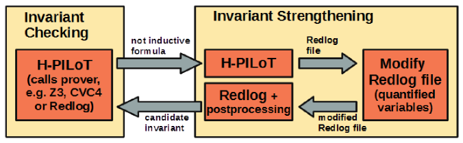
Figure 3: Current implementation of the algorithm

Figure 3 schematically shows our current implementation. Our invariant generation method consists of two steps (that are possibly repeated). We first check whether a candidate invariant is indeed an invariant (invariant checking), and if it is not we generate a stronger invariant (invariant strengthening).

For the invariant checking we only need to use H-PILoT. It can do the reduction and call a prover. If the answer is ”unsat”, we know that our candidate invariant is an inductive invariant. If the answer is ”sat”, then it is not an inductive invariant and we have to apply the invariant strengthening.

In the invariant strengthening step we first use H-PILoT to do the reduction, but we don’t let it call a prover. Instead we let it create an input file for Redlog. If we would call Redlog directly from H-PILoT, it would quantify all the variables. But since we only want to eliminate some of the variables, we have to modify the Redlog file accordingly (right now we have to do this manually, but we’d like to add to H-PILoT in the future the option to select certain variables that are to be eliminated by Redlog). We then use Redlog on the modified Redlog file. As a postprocessing step the output formula given by Redlog has to be negated. The conjunction of the old candidate invariant and the formulae obtained this way is the new candidate invariant.

7 Conclusion

We proposed a method for property-directed invariant generation and analyzed its properties.

We start from a given universal formula, describing a property of the data of the system. We can consider both properties on individual elements of an array (for instance: $a[i]\leq b[j]+c[k]$ for fixed indices $i,j,k$) and ”global properties”, for instance sortedness, or properties such as $\forall i(a[i]\leq b[i+1]-c[i-1]+d)$ (resp. e.g. $\forall i,j,k(a[i]\leq b[j]-c[k]-d)$ if we restrict to the array property fragment). These are properties which describe relationships which refer to the values of the variables or of the functions (e.g. arrays) at a given, fixed iteration in the execution of a loop. The invariants we generate have a similar form.

Our results extend the results in [Bra12] and [DDLM13], as we consider more complex theories. There are similarities to the method in [PIS⁺16], but our approach is different: The theories we analyze do not typically have the finite model property (required in [KBI⁺17, PIS⁺16] where, if a counterexample $A$ to the inductiveness of a candidate invariant $I$ is found, a formula is added to $I$ to avoid finding the same counterexample again in the next iteration; to construct this formula the finite model property assumption is used). In our work we use the symbol elimination method in Alg.1 to strengthen $I$; this should help to accelerate the procedure compared to the diagram-based approach. The decidability results in [PIS⁺16] are presented in a general framework and rely on the well-foundedness of certain relations. In this paper we consider extensions of arithmetic (or other theories allowing quantifier elimination) with additional function symbols; the theories we consider are not guaranteed to have the finite model property. For the situations in which we guarantee termination the abstract decidability or termination arguments in [PIS⁺16] might be difficult to check or might not hold (the arguments used for the case of pointers are not applicable). The algorithm proposed in [GR10] for the theories of arrays uses a non-deterministic function ChooseCover that returns a cover of a formula (as an approximation of the reachable states). It is proved that if the theory of elements is locally finite then for every universal formula $\Psi$, a universal inductive invariant $I$ strengthening $\Psi$ exists iff there exists a suitable ChooseCover function for which the algorithm returns an inductive invariant strengthening $\Psi$. In contrast to the algorithm proposed in [GR10], our algorithm is deterministic. To prove termination we show that the length of the quantifier prefix in the candidate invariants generated in every iteration does not grow; termination is then guaranteed if only finitely many atomic formulae formed with a fixed number of variables can be generated using quantifier elimination when applying the algorithm.

The methods used in [KV09b, KV09a, HKV10] and also in [GKR18] often introduce a new argument to constants and functions symbols. If $a(f)$ is $n$, then an $n+1$-ary version of $f$ is used; $f(x_{1},\dots,x_{n},i)$ denotes the value of $f(x_{1},\dots,x_{n})$ at iteration $i$. A major difference between our approach and the methods for invariant generation used in [KV09b, KV09a, HKV10] and [GKR18] is that we do not use additional indices to refer to the values of variables at iteration steps and do not quantify over the iteration steps. However, an extension with quantification over iteration steps and possibilities of giving explicit solutions to at least simple types of recurrences seems to be feasible.

Future work. We here restricted to universally quantified invariants and theories related to the array property fragment, but an extension to a framework using the notion of “extended locality” (cf. [IJS08, IS10]) seems unproblematic. We plan to identify additional situations in which our invariant generation method is correct, terminates resp. has low complexity – either by considering other theories or more general first-order properties.

Acknowledgments. We thank the reviewers of CADE-27 for their helpful comments.

Appendix A Proof of Theorem 12

Theorem 12. Let $\Psi\in{\sf LocSafe}$ and ${\sf Update}=\bigvee_{f\in F}{\sf Update}_{f}$ of the form discussed above. Assume that the clauses in $\Psi$ and ${\sf Update}_{f}$ are flat and linear for all $f\in F$. Let $m$ be the maximal number of variables in a clause in $\Psi$. Assume that the only non-parametric functions which need to be eliminated are the primed symbols $\{f^{\prime}\mid f\in F\}$ and that conditions (A1)–(A5) hold. Consider a variant of Algorithm 2, which uses for symbol elimination Algorithm 1 with the improvement in Theorem 5. Then for every step $n$, the clauses in the candidate invariant $I_{n}$ obtained at step $n$ of Algorithm 2 are flat, the number of universally quantified variables in every clause in $I_{n}$ is $\leq m$.

Proof: By Theorem 5, if the clauses ${\mathcal{K}}\cup I_{n}$ contain only function symbols in $\Sigma_{0}\cup\Sigma_{P}$, we need to apply Algorithm 1 to ${\sf Update}_{f}\wedge G$ only.

To prepare the formula for symbol elimination we compute $G_{1}={\sf Update}_{f}[G]\cup G$ (the extension terms used in the instantiation are est(G) = $\{f^{\prime}(d_{1}),\dots,f^{\prime}(d_{k})\}$), then instantiate also the terms starting with function symbols $g\in\Sigma_{P}\cup\Sigma$. Hence, we use the following set of ground terms: $T={\sf est}(G)\cup{\sf est}(G_{1})=\{f^{\prime}(d_{1}),\dots,f^{\prime}(d_{k})\}\cup\{g(c)\mid g\in\Sigma_{P}\cup\Sigma,g(c)\in{\sf est}(G_{1})\}$ (a set of flat terms, in which we isolated the terms starting with the function symbol $f$), By Lemma 11, we have:

$\begin{array}[]{@{}r@{}c@{}l}{\sf Update}_{f}[G]&:=&\displaystyle{\bigwedge_{j=1}^{k}\left(\bigwedge_{i=1}^{n_{f}}(\phi_{i}(d_{j})\rightarrow C_{i}(d_{j},f^{\prime}(d_{j})))\right)\equiv\bigwedge_{j=1}^{k}\bigvee_{i=1}^{n}(\phi_{i}(d_{j})\wedge C_{i}(d_{j},f^{\prime}(d_{j})))}\\ &\equiv&\displaystyle{\bigvee_{i_{1},\dots,i_{k}\in\{1,\dots,n_{f}\}}\left(\bigwedge_{p=1}^{k}\phi_{i_{p}}(d_{p})\wedge\bigwedge_{p=1}^{k}C_{i_{p}}(d_{p},f^{\prime}(d_{p}))\right).}\end{array}$

We thus obtained a DNF with $(n_{f})^{k}\leq(n_{f})^{m}$ disjuncts, where $n_{f}$ (number of cases in the definition of $f$) and $m$ (the maximal number of variables in ${\mathcal{K}}\cup I_{n}$) are constants depending on the description of the transition system. (We will show that this number does not increase in $\Gamma_{n+1}$.) Both $n_{f}$ and $m$ are typically small, in most cases $n_{f}\leq 3$.

Step 1: We introduce a constant $c_{f^{\prime}d}$ for every term $f^{\prime}(d)\in{\sf est}(G)$, replace $f^{\prime}(d)$ with $c_{f^{\prime}d}$, add the corresponding instances of the congruence axioms and obtain:

$$\begin{array}[]{rcll}G_{1}&=&G_{0}\wedge&({\sf Update}_{f}[G])_{0}\wedge\displaystyle{\bigwedge_{f^{\prime}(d_{1}),f^{\prime}(d_{2})\in{\sf est}(G)}d_{1}=d_{2}\rightarrow c_{f^{\prime}d_{1}}=c_{f^{\prime}d_{2}}}\end{array}$$

We may compute a disjunctive normal form for the instances of congruence axioms or not; depending on this we obtain one of the equivalences (1) or (2) below:

$$G_{1} \equiv G_{0}\wedge\!\!\!\!\!\!\!\!\!\!\displaystyle{\bigvee_{\stackrel{{\scriptstyle i_{1},\dots,i_{n}\in\{1,\dots,n_{f}\}}}{{D\subseteq{\sf est}(G)^{2}}}}}\bigg{(} \displaystyle{\bigwedge_{p=1}^{k}\phi_{i_{p}}(d_{p})\wedge\bigwedge_{p=1}^{k}C_{i_{p}}(d_{p},c_{f^{\prime}d_{p}})}\wedge K_{D}({\sf Con}_{0})\bigg{)}$$ (1)

$$\equiv G_{0}\wedge\!\!\!\!\!\!\!\!\!\!\displaystyle{\bigvee_{i_{1},\dots,i_{n}\in\{1,\dots,n_{f}\}}}\bigg{(} \displaystyle{\bigwedge_{p=1}^{k}\phi_{i_{p}}(d_{p})\wedge\bigwedge_{p=1}^{k}C_{i_{p}}(d_{p},c_{f^{\prime}d_{p}})}\wedge{\sf Con}_{0}\bigg{)}$$ (2)

In equivalence (1) we brought the formula to DNF. The formulae $K_{D}({\sf Con})$ are the conjunctions which appear when bringing the congruence axioms to DNF, based on a subset $D$ of ${\sf est}(G)^{2}$. In equivalence (2) we used distributivity and moved the conjunction of all congruence axioms inside the conjunctive formulae in the big disjunction.

Note that ${\sf Con}_{0}=\displaystyle{\bigwedge_{f(d_{1}),{f_{(}d_{2})}\in{\sf est}(G)}}(d_{1}=d_{2}\rightarrow c_{f^{\prime}d_{1}}=c_{f^{\prime}d_{2}})$ and every formula

$$K_{D}({\sf Con}_{0})=\displaystyle{\bigwedge_{(f(d_{1}),f(d_{2}))\in D}\!\!\!\!\!\!d_{1}\neq d_{2}\wedge\!\!\!\!\!\!\!\!\!\!\!\!\!\!\!\!\!\!\!\bigwedge_{(f^{\prime}(d_{1}),f^{\prime}(d_{2}))\in{\sf est}(G)^{2}\backslash D}\!\!\!\!\!\!\!\!\!\!\!\!\!\!\!\!\!\!c_{f^{\prime}d_{1}}=c_{f^{\prime}d_{2}}}$$

contain $k^{2}\leq m^{2}$ conjunctions.

In a second reduction we replace every term of the form $g(d)\in{\sf est}(G_{1})$, $g\in\Sigma_{P}$, with a new constant $c_{gd}$. By Theorem 5 we do not need to add the corresponding congruence axioms. Using equivalence (1) and distributivity we obtain:

$$G_{1(1)}^{0} \equiv \!\!\!\!\!\!\!\!\!\!\!\!\!\!\!\displaystyle{\bigvee_{\stackrel{{\scriptstyle i_{1},\dots,i_{k}\in\{1,\dots,n_{f}\}}}{{D\subseteq{\sf est}(G)^{2}}}}}\!\!\!\!\!~{}\bigg{(}\displaystyle{\bigwedge_{p=1}^{k}\phi^{0}_{i_{p}}(d_{p}){\wedge}\bigwedge_{p=1}^{k}C^{0}_{i_{p}}(d_{p},c_{f^{\prime}d_{p}})}{\wedge}K_{D}({\sf Con}_{0}){\wedge}G^{0}_{0}({\overline{d}},{\overline{c}},{\overline{c}_{f^{\prime}d}},{\overline{c}_{gc}})\bigg{)}$$ (3)

Using equivalence (2) and distributivity we obtain:

$$G_{1(2)}^{0} \equiv \!\!\!\!\!\!\!\!\!\!\displaystyle{\bigvee_{i_{1},\dots,i_{n}\in\{1,\dots,n_{f}\}}}\!\!\!\!\!~{}~{}\bigg{(}\displaystyle{\bigwedge_{p=1}^{k}\phi^{0}_{i_{p}}(d_{p})}{\wedge}\displaystyle{\bigwedge_{p=1}^{k}C^{0}_{i_{p}}(d_{p},c_{f^{\prime}d_{p}})}{\wedge}{\sf Con}_{0}{\wedge}G^{0}_{0}({\overline{d}},{\overline{c}},{\overline{c}_{f^{\prime}d}},{\overline{c}_{gc}})\bigg{)}$$ (4)

where $\phi_{j}^{0},C^{0}_{j},G_{0}^{0}$ are obtained from $\phi_{j},C_{j},G_{0}$ after replacing all terms of the form $g(c)$, $g\in\Sigma_{P}$ with $c_{gc}$.

Step 2: $f^{\prime}$ is not a parameter; all the other function symbols are either parametric or in ${\mathcal{T}}_{0}$. We therefore replace the constants $c_{f^{\prime}d}$ with variables $x_{f^{\prime}d}$.

Step 3: Note that $\exists x_{f^{\prime}d_{1}},\dots x_{f^{\prime}d_{n}}~{}G^{0}_{1(1)}(x_{f^{\prime}d_{1}},\dots,x_{f^{\prime}d_{n}})$ is equivalent to:

$$G^{\prime}_{1(1)} \equiv \!\!\!\!\!\!\!\!\!\!\displaystyle{\bigvee_{\stackrel{{\scriptstyle i_{1},\dots,i_{n}\in\{1,\dots,n_{f}\}}}{{D\subseteq{\sf est}(G)^{2}}}}}\!\!\!\!\!\!\!\!\!\!~{}~{}~{}~{}~{}\Bigg{(}\displaystyle{\bigwedge_{p=1}^{k}\phi^{0}_{i_{p}}(d_{p})\wedge\bigwedge_{(f^{\prime}(d_{1}),f^{\prime}(d_{2}))\in D}\!\!\!\!d_{1}\neq d_{2}}\wedge$$

$$\exists x_{f^{\prime}d_{1}},\dots x_{f^{\prime}d_{n}}\bigg{(}\displaystyle{\bigwedge_{p=1}^{k}C^{0}_{i_{p}}(d_{p},x_{f^{\prime}d_{p}})\wedge\!\!\!\!\!\!\!\!\!\!\!\!\!\!\bigwedge_{(f^{\prime}(d_{1}),f^{\prime}(d_{2}))\in{\sf est}(G)^{2}\backslash D}\!\!\!\!\!\!\!\!\!\!\!\!\!\!x_{f^{\prime}d_{1}}=x_{f^{\prime}d_{2}}}\wedge G^{0}_{0}({\overline{d}},{\overline{c}},{\overline{c}_{gc}},{\overline{x}_{f^{\prime}d}})\bigg{)}\Bigg{)}$$

Using equivalence (2) we obtain:

$$G^{\prime}_{1(2)} \equiv \!\!\!\!\!\!\!\!\!\!\displaystyle{\bigvee_{i_{1},\dots,i_{n}\in\{1,\dots,n_{f}\}}}\Bigg{(}\displaystyle{\bigwedge_{p=1}^{k}\phi^{0}_{i_{p}}(d_{p})}\wedge\exists x_{f^{\prime}d_{1}},\dots x_{f^{\prime}d_{n}}\bigg{(}\displaystyle{\bigwedge_{p=1}^{k}C^{0}_{i_{p}}(d_{p},x_{f^{\prime}d_{p}})}\wedge$$

$$\displaystyle{\!\!\!\!\!\!\!\!\!\!\!\!\!\!\bigwedge_{(f^{\prime}(d_{1}),f(^{\prime}d_{2}))\in{\sf est}(G)}\!\!\!\!(d_{1}=d_{2}\rightarrow x_{f^{\prime}d_{1}}=x_{f^{\prime}d_{2}})}\wedge G^{0}_{0}({\overline{d}},{\overline{c}},{\overline{c}_{gc}},{\overline{x}_{f^{\prime}d}})\bigg{)}\Bigg{)}$$

After quantifier elimination we obtain, using equivalence (1), a formula of the form:

$$G^{\prime\prime}_{1(1)} \equiv \!\!\!\!\!\!\!\!\!\!\displaystyle{\bigvee_{\stackrel{{\scriptstyle i_{1},\dots,i_{n}\in\{1,\dots,n_{f}\}}}{{D\subseteq{\sf est}(G)^{2}}}}}\bigg{(}\displaystyle{\bigwedge_{p=1}^{k}\phi^{0}_{i_{p}}(d_{p})\wedge\bigwedge_{(d_{1},d_{2})\in D}\!\!\!\!d_{1}\neq d_{2}}\wedge D^{1}_{i_{1},\dots,i_{n},D}({\overline{d}},{\overline{c}},{\overline{c}_{gc}})\bigg{)}$$ (7)

and using equivalence (2):

$$G^{\prime\prime}_{1(2)} \equiv \!\!\!\!\!\!\!\!\!\!\displaystyle{\bigvee_{i_{1},\dots,i_{n}\in\{1,\dots,n_{f}\}}\Bigg{(}\bigwedge_{p=1}^{k}\phi^{0}_{i_{p}}(d_{p})\wedge D^{2}_{i_{1},\dots,i_{n},D}({\overline{d}},{\overline{c}},{\overline{c}_{gc}})}\Bigg{)}$$ (8)

where $D^{1}_{i_{1},\dots,i_{n},D}({\overline{d}},{\overline{c}},{\overline{c}_{gc}})$ is obtained after QE from

$\exists x_{f^{\prime}d_{1}},\dots x_{f^{\prime}d_{n}}\bigg{(}\displaystyle{\bigwedge_{p=1}^{k}C^{0}_{i_{p}}(d_{p},x_{f^{\prime}d_{p}})\wedge\!\!\!\!\!\!\!\!\!\!\!\!\!\!\bigwedge_{(f^{\prime}(d_{1}),f^{\prime}(d_{2}))\in{\sf est}(G)^{2}\backslash D}\!\!\!\!\!\!x_{f^{\prime}d_{1}}=x_{f^{\prime}d_{2}}}\wedge G^{0}_{0}({\overline{d}},{\overline{c}},{\overline{c}_{gc}},{\overline{x}_{f^{\prime}d}})\bigg{)}$

and $D^{2}_{i_{1},\dots,i_{n},D}({\overline{d}},{\overline{c}},{\overline{c}_{gc}})$ is obtained after QE from

$\exists x_{f^{\prime}d_{1}},\dots x_{f^{\prime}d_{n}}\bigg{(}\displaystyle{\bigwedge_{p=1}^{k}C^{0}_{i_{p}}(d_{p},x_{f^{\prime}d_{p}})}\wedge\displaystyle{\!\!\!\!\!\!\!\!\!\!\!\!\!\!\bigwedge_{(f^{\prime}(d_{1}),f^{\prime}(d_{2}))\in{\sf est}(G)}\!\!\!\!\!\!\!\!(d_{1}=d_{2}\rightarrow x_{f^{\prime}d_{1}}=x_{f^{\prime}d_{2}})}\wedge G^{0}_{0}({\overline{d}},{\overline{c}},{\overline{c}_{gc}},{\overline{x}_{f^{\prime}d}})\bigg{)}.$

Step 4: We replace back in the formula obtained this way all constants $c_{gd}$, $g\in\Sigma_{P},g(c)\in{\sf est}(G_{1})$ with the terms $g(c)$. We obtain therefore, if starting from formula (1):

$\begin{array}[]{ll}\Gamma_{2(1)}({\overline{d}},{\overline{c}})=\!\!\!\!\!\!\!\!\!\!\displaystyle{\bigvee_{\stackrel{{\scriptstyle i_{1},\dots,i_{n}\in\{1,\dots,n_{f}\}}}{{D\subseteq{\sf est}(G)^{2}}}}}\Bigg{(}&\bigg{(}\displaystyle{\bigwedge_{p=1}^{k}\phi_{i_{p}}(d_{p})}\wedge\displaystyle{\bigwedge_{(d_{1},d_{2})\in D}\!\!\!\!d_{1}\neq d_{2}\wedge G^{g}_{0}({\overline{d}},{\overline{c}},{\overline{g}(c)})\bigg{)}}\wedge\\ &D^{1}_{i_{1},\dots,i_{n},D}({\overline{d}},{\overline{c}},{\overline{g}(c)})\Bigg{)}\end{array}$

and if starting from formula (2):

$\begin{array}[]{ll}\Gamma_{2(2)}({\overline{d}},{\overline{c}})=\!\!\!\!\!\!\!\!\!\!\displaystyle{\bigvee_{i_{1},\dots,i_{n}\in\{1,\dots,n_{f}\}}\bigvee_{D\subseteq{\sf est}(G)^{2}}}\Bigg{(}&\bigg{(}\displaystyle{\bigwedge_{p=1}^{k}\phi_{i_{p}}(d_{p})}\wedge G^{g}_{0}({\overline{d}},{\overline{c}},{\overline{g}(c)})\bigg{)}\wedge D^{2}_{i_{1},\dots,i_{n},D}({\overline{d}},{\overline{c}},{\overline{g}(c)})\Bigg{)}\end{array}$

Step 5: We negate $\exists{\overline{y}}\Gamma_{2(1)}({\overline{y}})$ and obtain:

$$\begin{array}[]{ll}\forall y\Bigg{[}\!\!\!\!\!\!\!\!\!\!\displaystyle{\bigwedge_{i_{1},\dots,i_{n}\in\{1,\dots,n_{f}\}}\bigwedge_{D\subseteq{\sf est}(G)^{2}}}\Bigg{(}&\neg\bigg{(}\displaystyle{\bigwedge_{p=1}^{k}\phi_{i_{p}}(y_{p})}\wedge\!\!\!\!\displaystyle{\bigwedge_{(f(d_{1}),f(d_{2}))\in D}}\!\!\!\!y_{1}\neq y_{2}\wedge G^{g}_{0}({\overline{y}},{\overline{g}(y)})\bigg{)}\wedge\\ &\neg D^{1}_{i_{1},\dots,i_{n},D}({\overline{y}},{\overline{g}(y)})\Bigg{)}\Bigg{]}\end{array}$$

which is equivalent with:

$$\begin{array}[]{ll}\forall y\Bigg{[}\!\!\!\!\!\!\!\!\!\!\displaystyle{\bigwedge_{i_{1},\dots,i_{n}\in\{1,\dots,n_{f}\}}\bigwedge_{D\subseteq{\sf est}(G)^{2}}}\Bigg{(}&\bigg{(}\displaystyle{\bigwedge_{p=1}^{k}\phi_{i_{p}}(y_{p})}\wedge\displaystyle{\bigwedge_{(f(d_{1}),f(d_{2}))\in D}}\!\!\!\!y_{1}\neq y_{2}\wedge G^{g}_{0}({\overline{y}},{\overline{g}(y)})\bigg{)}\wedge\\ &\rightarrow\neg D^{1}_{i_{1},\dots,i_{n},D}({\overline{y}},{\overline{g}(y)})\Bigg{)}\Bigg{]}\end{array}$$

Similarly for $\exists{\overline{y}}\Gamma_{2(2)}({\overline{y}})$.

Complexity: We analyze the complexity of the transformations presented above. We show how the size of the formula changes depending on $n_{f}$ and $m$ (since $k\leq m$ and $m$ is a constant of the system). After the instantiation we first have a conjunction of $k*n_{f}\leq m*n_{f}$ implications. After the transformation to DNF we obtain a disjunction of at most $n_{f}^{m}$ conjunctions, each of length at most $m*l_{f}$, where $l_{f}$ is the maximal length of a rule in ${\sf Update}_{f}$. After applying the first reduction in Step 1 we obtain a disjunction of $n_{f}^{m}*2^{m^{2}}$ conjunctions each of length at most $(m*l_{f}+m^{2}+|G|)$ (with transformation (1)) resp. of $n_{f}$ formulae, each of length at most $(m*l_{f}+|G|+|{\sf Con}_{0}|)$ (with transformation (2)). Note that $m*l_{f}$ and $m^{2}$ are constants of the system. In Step 2 the size of the formulae does not change. After quantifier elimination in Step 3 the size of the conjuncts may grow: for every variable which is eliminated, the size of the formula might grow quadratically. The last two steps of the algorithm do not change the size of the formula.

References

- [ABG+14] Francesco Alberti, Roberto Bruttomesso, Silvio Ghilardi, Silvio Ranise, and Natasha Sharygina. An extension of lazy abstraction with interpolation for programs with arrays. Formal Methods in System Design, 45(1):63–109, 2014.
- [BGR14] Roberto Bruttomesso, Silvio Ghilardi, and Silvio Ranise. Quantifier-free interpolation in combinations of equality interpolating theories. ACM Trans. Comput. Log., 15(1):5:1–5:34, 2014.
- [BGW94] Leo Bachmair, Harald Ganzinger, and Uwe Waldmann. Refutational theorem proving for hierarchic first-order theories. Appl. Algebra Eng. Commun. Comput., 5:193–212, 1994.
- [BHMR07] Dirk Beyer, Thomas A. Henzinger, Rupak Majumdar, and Andrey Rybalchenko. Invariant synthesis for combined theories. In Byron Cook and Andreas Podelski, editors, Verification, Model Checking, and Abstract Interpretation, 8th International Conference, VMCAI 2007, Nice, France, January 14-16, 2007, Proceedings, volume 4349 of Lecture Notes in Computer Science, pages 378–394. Springer, 2007.
- [BM08] Aaron R. Bradley and Zohar Manna. Property-directed incremental invariant generation. Formal Asp. Comput., 20(4-5):379–405, 2008.
- [BMS06] Aaron R. Bradley, Zohar Manna, and Henny B. Sipma. What’s decidable about arrays? In E. Allen Emerson and Kedar S. Namjoshi, editors, Verification, Model Checking, and Abstract Interpretation, 7th International Conference, VMCAI 2006, Charleston, SC, USA, January 8-10, 2006, Proceedings, volume 3855 of Lecture Notes in Computer Science, pages 427–442. Springer, 2006.
- [Bra12] Aaron R. Bradley. IC3 and beyond: Incremental, inductive verification. In P. Madhusudan and Sanjit A. Seshia, editors, Computer Aided Verification - 24th International Conference, CAV 2012, Berkeley, CA, USA, July 7-13, 2012 Proceedings, volume 7358 of Lecture Notes in Computer Science, page 4. Springer, 2012.
- [Bro04] Christopher W. Brown. QEPCAD B: a system for computing with semi-algebraic sets via cylindrical algebraic decomposition. ACM SIGSAM Bulletin, 38(1):23–24, 2004.
- [CGK+12] Sylvain Conchon, Amit Goel, Sava Krstic, Alain Mebsout, and Fatiha Zaïdi. Cubicle: A parallel smt-based model checker for parameterized systems - tool paper. In P. Madhusudan and Sanjit A. Seshia, editors, Computer Aided Verification - 24th International Conference, CAV 2012, Berkeley, CA, USA, July 7-13, 2012 Proceedings, volume 7358 of Lecture Notes in Computer Science, pages 718–724. Springer, 2012.
- [DDLM13] Isil Dillig, Thomas Dillig, Boyang Li, and Kenneth L. McMillan. Inductive invariant generation via abductive inference. In Antony L. Hosking, Patrick Th. Eugster, and Cristina V. Lopes, editors, Proceedings of the 2013 ACM SIGPLAN International Conference on Object Oriented Programming Systems Languages & Applications, OOPSLA 2013, part of SPLASH 2013, Indianapolis, IN, USA, October 26-31, 2013, pages 443–456. ACM, 2013.
- [DS97] Andreas Dolzmann and Thomas Sturm. Redlog: Computer algebra meets computer logic. ACM SIGSAM Bulletin, 31(2):2–9, 1997.
- [FJS07] Johannes Faber, Swen Jacobs, and Viorica Sofronie-Stokkermans. Verifying CSP-OZ-DC specifications with complex data types and timing parameters. In Jim Davies and Jeremy Gibbons, editors, Integrated Formal Methods, 6th International Conference, IFM 2007, Oxford, UK, July 2-5, 2007, Proceedings, volume 4591, pages 233–252. Springer, 2007.
- [FK15] Stephan Falke and Deepak Kapur. When is a formula a loop invariant? In Narciso Martí-Oliet, Peter Csaba Ölveczky, and Carolyn L. Talcott, editors, Logic, Rewriting, and Concurrency - Essays dedicated to José Meseguer on the Occasion of His 65th Birthday, volume 9200 of Lecture Notes in Computer Science, pages 264–286. Springer, 2015.
- [GKR18] Bernhard Gleiss, Laura Kovács, and Simon Robillard. Loop analysis by quantification over iterations. In Gilles Barthe, Geoff Sutcliffe, and Margus Veanes, editors, LPAR-22. 22nd International Conference on Logic for Programming, Artificial Intelligence and Reasoning, Awassa, Ethiopia, 16-21 November 2018, volume 57 of EPiC Series in Computing, pages 381–399. EasyChair, 2018.
- [GR10] Silvio Ghilardi and Silvio Ranise. Backward reachability of array-based systems by SMT solving: Termination and invariant synthesis. Logical Methods in Computer Science, 6(4), 2010.
- [GSV18] Arie Gurfinkel, Sharon Shoham, and Yakir Vizel. Quantifiers on demand. In Shuvendu K. Lahiri and Chao Wang, editors, Automated Technology for Verification and Analysis - 16th International Symposium, ATVA 2018, Los Angeles, CA, USA, October 7-10, 2018, Proceedings, volume 11138 of Lecture Notes in Computer Science, pages 248–266. Springer, 2018.
- [GSW04] Harald Ganzinger, Viorica Sofronie-Stokkermans, and Uwe Waldmann. Modular proof systems for partial functions with weak equality. In David A. Basin and Michaël Rusinowitch, editors, Automated Reasoning - Second International Joint Conference, IJCAR 2004, Cork, Ireland, July 4-8, 2004, Proceedings, volume 3097 of Lecture Notes in Computer Science, pages 168–182. Springer, 2004.
- [GSW06] Harald Ganzinger, Viorica Sofronie-Stokkermans, and Uwe Waldmann. Modular proof systems for partial functions with evans equality. Inf. Comput., 204(10):1453–1492, 2006.
- [HKV10] Krystof Hoder, Laura Kovács, and Andrei Voronkov. Interpolation and symbol elimination in vampire. In Jürgen Giesl and Reiner Hähnle, editors, Automated Reasoning, 5th International Joint Conference, IJCAR 2010, Edinburgh, UK, July 16-19, 2010. Proceedings, volume 6173 of Lecture Notes in Computer Science, pages 188–195. Springer, 2010.
- [HS13] Matthias Horbach and Viorica Sofronie-Stokkermans. Obtaining finite local theory axiomatizations via saturation. In Pascal Fontaine, Christophe Ringeissen, and Renate A. Schmidt, editors, Frontiers of Combining Systems - 9th International Symposium, FroCoS 2013, Nancy, France, September 18-20, 2013. Proceedings, volume 8152 of Lecture Notes in Computer Science, pages 198–213. Springer, 2013.
- [HS14] Matthias Horbach and Viorica Sofronie-Stokkermans. Locality transfer: From constrained axiomatizations to reachability predicates. In Stéphane Demri, Deepak Kapur, and Christoph Weidenbach, editors, Automated Reasoning - 7th International Joint Conference, IJCAR 2014, Held as Part of the Vienna Summer of Logic, VSL 2014, Vienna, Austria, July 19-22, 2014. Proceedings, volume 8562 of Lecture Notes in Computer Science, pages 192–207. Springer, 2014.
- [HW09] Matthias Horbach and Christoph Weidenbach. Deciding the inductive validity of FOR ALL THERE EXISTS queries. In Erich Grädel and Reinhard Kahle, editors, Computer Science Logic, 23rd international Workshop, CSL 2009, 18th Annual Conference of the EACSL, Coimbra, Portugal, September 7-11, 2009. Proceedings, volume 5771 of Lecture Notes in Computer Science, pages 332–347. Springer, 2009.
- [IJS08] Carsten Ihlemann, Swen Jacobs, and Viorica Sofronie-Stokkermans. On local reasoning in verification. In C. R. Ramakrishnan and Jakob Rehof, editors, Tools and Algorithms for the Construction and Analysis of Systems, 14th International Conference, TACAS 2008, Held as Part of the Joint European Conferences on Theory and Practice of Software, ETAPS 2008, Budapest, Hungary, March 29-April 6, 2008. Proceedings, volume 4963 of Lecture Notes in Computer Science, pages 265–281. Springer, 2008.
- [Inc] Wolfram Research, Inc. Mathematica, Version 12.0. Champaign, IL, 2019.
- [IS09] Carsten Ihlemann and Viorica Sofronie-Stokkermans. System description: H-PILoT. In Renate A. Schmidt, editor, Automated Deduction - CADE-22, 22nd International Conference on Automated Deduction, Montreal, Canada, August 2-7, 2009. Proceedings, volume 5663 of Lecture Notes in Computer Science, pages 131–139. Springer, 2009.
- [IS10] Carsten Ihlemann and Viorica Sofronie-Stokkermans. On hierarchical reasoning in combinations of theories. In Jürgen Giesl and Reiner Hähnle, editors, Automated Reasoning, 5th International Joint Conference, IJCAR 2010, Edinburgh, UK, July 16-19, 2010. Proceedings, volume 6173 of Lecture Notes in Computer Science, pages 30–45. Springer, 2010.
- [JK11] Swen Jacobs and Viktor Kuncak. Towards complete reasoning about axiomatic specifications. In Ranjit Jhala and David A. Schmidt, editors, Verification, Model Checking, and Abstract Interpretation - 12th International Conference, VMCAI 2011, Austin, TX, USA, January 23-25, 2011. Proceedings, volume 6538 of Lecture Notes in Computer Science, pages 278–293. Springer, 2011.
- [Kap06] Deepak Kapur. A quantifier-elimination based heuristic for automatically generating inductive assertions for programs. J. Systems Science & Complexity, 19(3):307–330, 2006.
- [KBI+17] Aleksandr Karbyshev, Nikolaj Bjørner, Shachar Itzhaky, Noam Rinetzky, and Sharon Shoham. Property-directed inference of universal invariants or proving their absence. J. ACM, 64(1):7:1–7:33, 2017.
- [KMZ06] Deepak Kapur, Rupak Majumdar, and Calogero G. Zarba. Interpolation for data structures. In Michal Young and Premkumar T. Devanbu, editors, Proceedings of the 14th ACM SIGSOFT International Symposium on Foundations of Software Engineering, FSE 2006, Portland, Oregon, USA, November 5-11, 2006, pages 105–116. ACM, 2006.
- [KV09a] Laura Kovács and Andrei Voronkov. Finding loop invariants for programs over arrays using a theorem prover. In Marsha Chechik and Martin Wirsing, editors, Fundamental Approaches to Software Engineering, 12th International Conference, FASE 2009, Held as Part of the Joint European Conferences on Theory and Practice of Software, ETAPS 2009, York, UK, March 22-29, 2009. Proceedings, volume 5503 of Lecture Notes in Computer Science, pages 470–485. Springer, 2009.
- [KV09b] Laura Kovács and Andrei Voronkov. Interpolation and symbol elimination. In Renate A. Schmidt, editor, Automated Deduction - CADE-22, 22nd International Conference on Automated Deduction, Montreal, Canada, August 2-7, 2009. Proceedings, volume 5663 of Lecture Notes in Computer Science, pages 199–213. Springer, 2009.
- [PIS+16] Oded Padon, Neil Immerman, Sharon Shoham, Aleksandr Karbyshev, and Mooly Sagiv. Decidability of inferring inductive invariants. In Rastislav Bodík and Rupak Majumdar, editors, Proceedings of the 43rd Annual ACM SIGPLAN-SIGACT Symposium on Principles of Programming Languages, POPL 2016, St. Petersburg, FL, USA, January 20 - 22, 2016, pages 217–231. ACM, 2016.
- [PSS19] Dennis Peuter and Viorica Sofronie-Stokkermans. On invariant synthesis for parametric systems. In Pascal Fontaine, editor, Proceedings of CADE-2019. Springer, 2019. To appear.
- [Sof05] Viorica Sofronie-Stokkermans. Hierarchic reasoning in local theory extensions. In Robert Nieuwenhuis, editor, Automated Deduction - CADE-20, 20th International Conference on Automated Deduction, Tallinn, Estonia, July 22-27, 2005, Proceedings, volume 3632 of Lecture Notes in Computer Science, pages 219–234. Springer, 2005.
- [Sof06] Viorica Sofronie-Stokkermans. Interpolation in local theory extensions. In Ulrich Furbach and Natarajan Shankar, editors, Automated Reasoning, Third International Joint Conference, IJCAR 2006, Seattle, WA, USA, August 17-20, 2006, Proceedings, volume 4130 of Lecture Notes in Computer Science, pages 235–250. Springer, 2006.
- [Sof08] Viorica Sofronie-Stokkermans. Interpolation in local theory extensions. Logical Methods in Computer Science, 4(4), 2008.
- [Sof10] Viorica Sofronie-Stokkermans. Hierarchical reasoning for the verification of parametric systems. In Jürgen Giesl and Reiner Hähnle, editors, Automated Reasoning, 5th International Joint Conference, IJCAR 2010, Edinburgh, UK, July 16-19, 2010. Proceedings, volume 6173 of Lecture Notes in Computer Science, pages 171–187. Springer, 2010.
- [Sof13] Viorica Sofronie-Stokkermans. Hierarchical reasoning and model generation for the verification of parametric hybrid systems. In Maria Paola Bonacina, editor, Automated Deduction - CADE-24 - 24th International Conference on Automated Deduction, Lake Placid, NY, USA, June 9-14, 2013. Proceedings, volume 7898 of Lecture Notes in Computer Science, pages 360–376. Springer, 2013.
- [Sof16] Viorica Sofronie-Stokkermans. On interpolation and symbol elimination in theory extensions. In Nicola Olivetti and Ashish Tiwari, editors, Automated Reasoning - 8th International Joint Conference, IJCAR 2016, Coimbra, Portugal, June 27 - July 2, 2016, Proceedings, volume 9706 of Lecture Notes in Computer Science, pages 273–289. Springer, 2016.
- [SS18] Viorica Sofronie-Stokkermans. On Interpolation and Symbol Elimination in Theory Extensions. Logical Methods in Computer Science, Volume 14, Issue 3, September 2018.
- [YM05] Greta Yorsh and Madanlal Musuvathi. A combination method for generating interpolants. In Robert Nieuwenhuis, editor, Automated Deduction - CADE-20, 20th International Conference on Automated Deduction, Tallinn, Estonia, July 22-27, 2005, Proceedings, volume 3632 of Lecture Notes in Computer Science, pages 353–368. Springer, 2005.