Thermal Tensor Network Simulations of the Heisenberg Model on the Bethe Lattice
Abstract
We have extended the canonical tree tensor network (TTN) method, which was initially introduced to simulate the zero-temperature properties of quantum lattice models on the Bethe lattice, to finite temperature simulations. By representing the thermal density matrix with a canonicalized tree tensor product operator, we optimize the TTN and accurately evaluate the thermodynamic quantities, including the internal energy, specific heat, and the spontaneous magnetization, etc, at various temperatures. By varying the anisotropic coupling constant , we obtain the phase diagram of the spin-1/2 Heisenberg XXZ model on the Bethe lattice, where three kinds of magnetic ordered phases, namely the ferromagnetic, XY and antiferromagnetic ordered phases, are found in low temperatures and separated from the high- paramagnetic phase by a continuous thermal phase transition at . The XY phase is separated from the other two phases by two first-order phase transition lines at the symmetric coupling points . We have also carried out a linear spin wave calculation on the Bethe lattice, showing that the low-energy magnetic excitations are always gapped, and find the obtained magnon gaps in very good agreement with those estimated from the TTN simulations. Despite the gapped excitation spectrum, Goldstone-like transverse fluctuation modes, as a manifestation of spontaneous continuous symmetry breaking, are observed in the ordered magnetic phases with . One remarkable feature there is that the prominent transverse correlation length reaches for , the maximal value allowed on a -coordinated Bethe lattice.
I Introduction
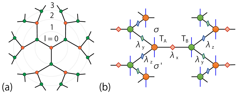
The Bethe approximation, a renowned cluster mean-field approach proposed by Bethe in 1935 Bethe (1935), has played an important role in the studies of cooperative phenomena and phase transitions of classical statistical models Pathria and Beale (2011). This approximation can be rigorously formulated on an ideal lattice of infinite Hausdorff dimension, i.e, the Bethe lattice shown in Fig. 1(a) Ostilli (2012). The Bethe lattice is also intimately connected with the dynamical mean-field theory Eckstein et al. (2005); Petrova and Moessner (2016); Semerjian et al. (2009).
A Bethe lattice is a loop-free graph where each site is connected to neighbours, i.e., is the coordination number. Figure 1(a), as an example, shows the structure of a Bethe lattice, whose lattice sites are all equivalent and there exists no boundary on this infinite lattice. This Bethe lattice resembles a two-dimensional honeycomb lattice locally [as emphasized in Fig. 1(b)], but it does not contain any closed loops, e.g., hexagons. A Bethe lattice becomes a Cayley tree if the lattice size is finite, where the sites are arranged in shells around a root site. In stark contrast to the Bethe lattice, there exist boundary sites, which are as many as the bulk sites, on the Cayley tree.
Tensor networks provide efficient and accurate representations of quantum manybody states both at zero and finite temperatures. The simple update Jiang et al. (2008), together with many other optimization schemes Verstraete et al. (2008); Orús (2014), has been widely adopted in the tensor-network simulations of quantum lattice models Li et al. (2012, 2010); Liu et al. (2014, 2015, 2016). It has also been shown that the simple update Jiang et al. (2008), or more rigorously the canonical tree tensor network (TTN) method, is numerically exact on the Bethe lattice Li et al. (2012). In addition, the density matrix renormalization group (DMRG) has also been employed to study the magnetic orders and other physical properties of the Heisenberg model on the Cayley tree Otsuka (1996); Friedman (1997); Kumar et al. (2012); Changlani et al. (2013a, b). Besides, the Bethe approximation has also been used in investigating the Fermi-Hubbard systems, where the single-particle Green’s function as well as the density of states are calculated Brinkman and Rice (1970); Kittler and Falicov (1976); Brouers and Marconi (1982). However, most of these studies are restricted in the properties, and there have not much investigations on the thermodynamic properties of quantum lattice models on the Bethe lattice.
In this paper, we extend the TTN approach from zero to finite temperatures and show that it provides an efficient and accurate method to simulate the thermodynamic properties of the Bethe-lattice quantum lattice models. Through the calculations of magnetic order parameters, we obtain the finite-temperature phase diagram of the anisotropic Heisenberg model. Similar as in the two-dimensional honeycomb lattice, three different magnetic ordered phases, i.e., the ferromagnetic (FM), antiferromagnetic (AF), and planar XY phases, are found on the Bethe lattice. The planar XY phase is separated from the FM and AF phases by two first-order phase transition lines at and , respectively, again resembling the two-dimensional case Al Hajj et al. (2004).
The correlation length, as shown in Ref. Li et al. (2012), is finite on a Bethe lattice. Here we show that a thermal phase transition can nevertheless happen when the correlation length reaches a “critical” value on the Bethe lattice. As revealed by the temperature dependence of thermodynamic quantities in low temperatures, the low-energy excitations of the XXZ model are always gapped. We propose a linear spin wave theory (LSWT) on the Bethe lattice, which gives insight into the low-energy excitations of the system and provides good estimates of the magnon gaps.
The paper is organized as follows. In Sec. II, we briefly introduce the Heisenberg XXZ model and the canonical TTN method on the Bethe lattice. The results obtained with this method are presented in Sec. III. In Sec. IV, we present a spin wave analysis of the model based on the -representation. Finally, in Sec. V, we summarize and discuss about further applications of the method introduced in this work.
II Interacting Spin Model and Tensor Network Method
II.1 The Heisenberg XXZ model
The Hamiltonian of Heisenberg XXZ model reads
| (1) |
where is the anisotropic coupling constant, and denotes a pair of nearest-neighboring sites. represents an external magnetic field, which is set as zero if not mentioned explicitly. Note the model with is equivalent to the isotropic FM Heisenberg model upon a -rotation around the -axis on one of the two sublattices, labelled by green and orange colors in Fig. 1(a), respectively. In the discussions below, we concentrate on the XXZ model defined on a Bethe lattice of coordination number .
II.2 Canonical TTN representation of the density matrix
As shown in Fig. 1(b), the density matrix on the Bethe lattice can be expressed as a TTN. A local tensor defined at a node contains two physical bonds, labelled by and , representing respectively the initial and final states of the density matrix. There are three geometric bonds, labelled by (), through which the network is connected. Besides this, there is also a vector or diagonal matrices defined on each internal bond , whose square (i.e., ) represents the entanglement spectra between the two blocks that are separated by this bond.
Given a density matrix, its TTN representation is not uniquely determined. By inserting a pair of invertible matrices, and its inverse , on each internal bond, we do not alter the density matrix. Hence, the TTN representations contain huge gauge redundancy. Nevertheless, the gauge degree of freedom can be fixed by converting a TTN into a canonical form, in which the local tensors ’s and diagonal bond matrices ’s satisfy a set of canonical equations. Taking the bond as an example, the canonical equation is
| (2) |
where or , representing the two sublattices of the Bethe lattice, is the dimension of the local basis states of spin-1/2, and is a identity matrix, with the dimension of geometric bond. The canonical equations along the and bonds can be obtained from Eq. (2) through a cyclic permutation of , , and . This kind of canonical form has already been used in one-dimensional tensor network algorithms, including the density matrix renormalization group (DMRG) White (1992), time-evolution block decimation Vidal (2007); Orús and Vidal (2008), and linearized tensor renormalization group Li et al. (2011); Dong et al. (2017), etc.
Given an arbitrary TTN representation which generically does not satisfy these canonical equations, we can nevertheless gauge the TTN into the canonical form through a so-called canonicalization procedure elaborated in App. A.2.
II.3 Imaginary-time evolution
The tensor network representation of thermal density matrix Li et al. (2011); Ran et al. (2012); Chen et al. (2017); Dong et al. (2017); Chen et al. (2018); Czarnik et al. (2012); Czarnik and Dziarmaga (2015); Czarnik et al. (2016, 2017); Kshetrimayum et al. (2019); Czarnik et al. (2019); Czarnik and Corboz can be determined by taking an imaginary-time evolution, starting from an infinitely high temperature at which is represented by the identity operator. This is achieved by taking a Trotter-Suzuki decomposition for the density matrix
| (3) | |||||
| (4) |
where is the inverse temperature and . is the interacting Hamiltonian between (nearest-neighboring) sites and along (=) directions. In practical calculations, the Trotter step is set as a small value, e.g., , to control the Trotter error. For the model we study, all the local terms in each commute with each other, i.e., , thus we can further decompose into a product of local evolution gates, i.e.,
A detailed introduction to the update scheme of local tensors in the imaginary-time evolution is given in App. A.1.
We dub the simple update equipped with the canonicalization procedure (App. A.2) as canonical TTN scheme on the Bethe lattice. The canonical TTN approach adopted in the present work indeed improves the accuracy and stability of the calculations, especially for the case with a thermal phase transition, as benchmarked in App. A.3.
After obtaining the tensor network representation, to evaluate thermodynamic quantities, we notice that the density matrix opertor is a product of two half density matrix operators
| (5) |
This TTN operator can be also regarded as a “supervector” , defined in the (enlarged) product space of the “ket” and “bra” spaces. In this supervector representation, the partition function then becomes an inner product of and its vector conjugate, namely
| (6) |
Thus the partition function can be obtained by contracting a bilayer TTN Dong et al. (2017).
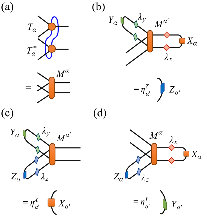
On the Bethe lattice, contracting the above bilayer supervectors is equivalent to solving the dominant eigen-problem of the transfer tensor defined by
| (7) |
whose schematic representation is shown Fig. 2(a). Supposing that , and are the three dominant eigenvectors to find, ( or ) simply transfers two of these eigenvectors in one of the sublattice to an eigenvector in the other sublattice, see Figs. 2(b-d). For example, transfers to through the equation [Fig. 2(b)],
| (8) |
where . This defines a generalized eigenvalue problem associated with the transfer tensor and can be solved iteratively, i.e., we start from six random vectors and perform the contractions until all vectors converge.
In stark contrast to the conventional linear eigenvalue problem, there is a gauge flexibility in the definition of eigenvalues here. Once the normalization condition of eigenvectors , and is varied, the corresponding eigenvalues also change, i.e, they are not uniquely defined. In the following, we fix the gauge by normalizing all the dominating eigenvectors to 1, e.g., . This is a convenient choice, and note that once the density matrix is in the canonical form, c.f., Eq. (2), the above iterative contraction procedures can be skipped, since each dominant eigenvector is just identity matrices if represented as a matrix.
Given the eigenvectors , and , we can evaluate the thermal expectation values of local operators, such as the local magnetization. For example, to evalueate the expectation value of an operator on the -sublattice, we first construct the single-site reduced density matrix
| (9) | |||||
The expectation value is then given by
| (10) |
which no longer depends on how the generalized dominant eigenvectors are normalized, since appears in both the numerator and the denominator. Similarly, we can evaluate the bond energies from the two-site reduced density matrix, etc.
From the canonical TTN, we can also calculate the bipartite-entanglement entropy using the normalized entanglement spectrum , as
| (11) |
which reflects both the quantum entanglement and classical correlations in a thermal equilibrium state. For gapless systems, the entanglement might exhibit a universal logarithmic scaling as a function of temperatures at low , e.g., in the one-dimensional quantum critical points and two-dimensional Heisenberg models Prosen and Pižorn (2007); Barthel ; Dubail ; Chen et al. (2018, 2019).
Therefore, it is of great interest to explore the scaling behaviors of , particularly near the phase transition temperatures, for the XXZ model on the Bethe lattice. Note, provides a quantitive measure of the bond dimension that is needed for an accurate representation of the thermal density matrix, especially in low temperatures. Generically, the bond dimension scales exponentially with , which would be saturated at low temperatures in a gapped system. On the contrary, in a gapless system would scale algebraically with inverse temperature , given that .
III Numerical results
Here we present the thermodynamic results calculated with the canonical TTN method. In our calculations, up to states are retained in the geometric bonds of local tensors to ensure that the results are converged down to .
To benchmark the method, we have evaluated the thermodynamic quantities with the canonical TTN in the classical limit [see Eq. (1)], at which the XXZ model is reduced to the exactly soluble Ising model. In this limit, the density matrix has an exact TTN representation with a bond dimension . We find that our numerical results agree excellently with the exact values. One can refer to App. B for details. Below, we show our TTN results of the quantum XXZ model at finite .
III.1 Phase diagram
It has been well-established that on a two-dimensional bipartite lattice, say, the honeycomb or square lattice, the XXZ model with breaks the continuous symmetry and possesses a long-range order in the ground state. However, at finite temperatures, the continuous symmetry is restored and the long-range magnetic order is melted by the low-lying excitations according to the Mermin-Wagner theorem Mermin and Wagner (1966).
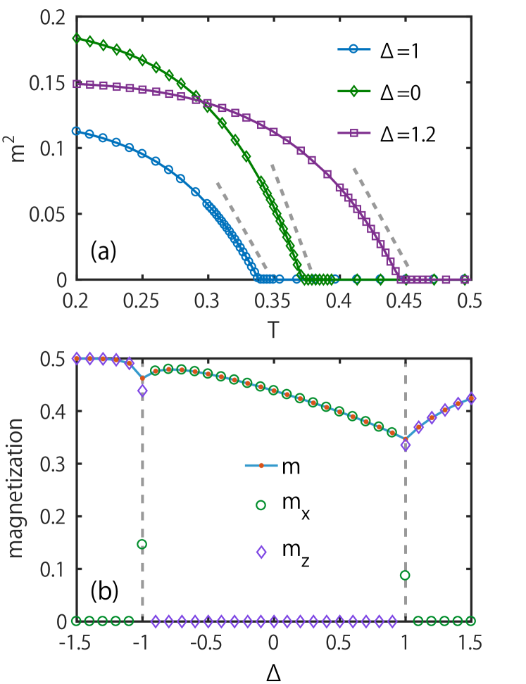
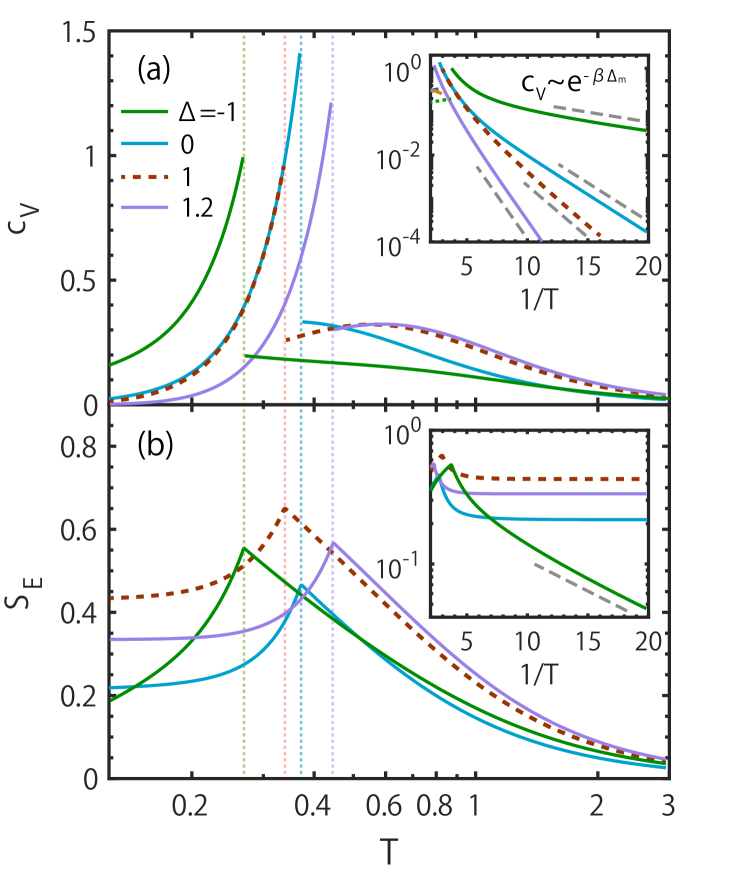
Figure 3 shows the temperature dependence of the magnetic order parameter
| (12) |
where and are the components within and perpendicular to the XY plane ( by default), respectively. The absolute values of are the same on the and sublattices, and there is no spontaneous symmetry breaking, i.e., , in high temperatures. However, becomes finite when the temperature drops below a critical value . Particularly, we find that varies linearly with temperature just below , i.e.,
We have checked three cases shown in Fig. 3(a) with , and , which all fall into this scalings in the vicinity of , thus indicating that the transition is mean-field-like.
Figure 4(a) shows the temperature dependence of the specific heat at several different values. A -jump is observed at the critical point , which confirms that the transition from the paramagnetic to magnetic-ordered phase is continuous (in a mean-field-like fashion). On the other hand, as shown in Fig. 4(b), the entanglement entropy curve vs. temperature exhibits a cusp, rather than a diverging peak, at . The absence of divergent at is a natural consequence of the finite correlation length in the system (see discussions on in Sec. III.2 below). It allows us to perform accurate thermal simulations down to low temperatures, , by retaining a finite number of bond states.
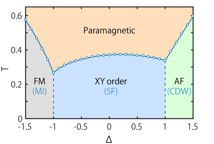
Figure 5 shows the - phase diagram of the Heisenberg XXZ model on the Bethe lattice, where three magnetic ordered phases are observed in low temperatures, by varying the anisotropic parameter . As depicted in Fig. 3(b), for and , the low-temperature states are AF and FM ordered, respectively. The system spontaneously breaks the symmetry, as characterized by and . When , the planar U(1) symmetry is broken, with and in low temperatures. This is in stark contrast to the corresponding two-dimensional lattice models with the same parameter, where no long-range order exists at any finite temperature according to the Mermin-Wagner theorem.
On the two vertical phase boundaries (marked by the two dashed lines in Fig. 5), both and become finite, but their ratio is somewhat arbitrary. This indicates that the system is in a random mixture of -symmetry-breaking AF (or FM) and U(1)-symmetry-breaking XY phases. In other words, the U(1) symmetry at or the SU(2) symmetry at is broken, and the transitions from the planar-XY order to either FM- or AF-ordered phase is of the first order. Both and become discontinuous at , while remains continuous across these two high-symmetry points.
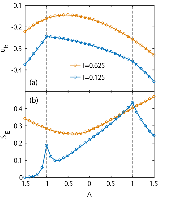
These two first-order phase transition lines can also be identified via other thermal measurements. Figure 6(a) shows the energy per bond as a function of in the high-temperature paramagnetic phase with , and deep in the symmetry-breaking phase with . At , the curve shows two turning points at , where the derivative becomes discontinuous, as a consequence of the first-order phase transitions. On the other hand, at , both and vary smoothly, suggesting the absence of phase transitions vs. .
Similarly, the phase transitions among these three phases can be seen from the -dependence of the entanglement entropy . As shown in Fig. 6(b), exhibits two peaks at at low temperature , which also becomes smooth at a high value .
Lastly, the XXZ spin model can be mapped onto a hardcore boson model with nearest-neighboring (NN) interactions, by setting and , where is a hardcore boson operator. In the boson language, the XY phase corresponds to a superfluid phase (SF) with an off-diagonal long-range order, and the FM and AF phases correspond to a Mott insulator (MI) and a charge density wave (CDW) phases, respectively. Along the two vertical phase boundary lines from low temperatures up to , the SF phase coexists with the MI or CDW phases.
III.2 Low-lying excitations and quasi-Goldstone modes
From the inset of Fig. 4(a), it is clear that the specific heat decays exponentially with in low temperatures, no matter in which magnetically ordered phase, i.e.,
| (13) |
This indicates that there is a finite excitation gap in the low-lying energy spectrum, quantified by the exponent in the above equation. The values of (Table 1) can be obtained by fitting the low- results of the specific heat or the internal energy . For example, for the FM phase at , the low-temperature internal energy is approximately described by the formula
| (14) |
where is the ground state energy per site, and is an external magnetic field, and is some polynomial prefactor. From the derivative of this equation
and through a polynomial fitting, the magnon gap can be readily read out from the intercept at . Moreover, for this FM system, one can further tune the magnon gap by changing the external magnetic fields . The FM excitation gaps of various (small) magnetic fields are also obtained by fitting the internal energy curves and shown in Table 1, from which we find that . This suggests that the elementary excitations in the FM phase are magnons with spin .
To further clarify the nature of low-lying excitations, we have evaluated the correlation length from the transfer matrix along the path on the Bethe lattice, meaning going through the bond of the tensor to , and then through its bond to the next , and so on. There are also other paths that can be used to define the transfer matrix. But all these paths are physically equivalent and the correlation lengths obtained thereof are also found exactly the same.
Suppose and are the dominant and the ()’th largest eigenvalue of the transfer matrix, the correlation length can be determined as
| (15) |
where is the largest correlation length the system can have, and is related to a shorter-ranged correlation function.
| Model | (, ) | (TTN, fitted) | (LSWT, ) |
| AF | (1, 0) | 0.56(3) | |
| XY | (0, 0) | 0.41(1) | |
| FM | (-1, 0) | 0.085(3) | |
| (-1, 0.1) | 0.186(1) | ||
| (-1, 0.2) | 0.286(2) |
Alternatively, one can also estimate the correlation length directly from the real-space spin-spin correlation function
| (16) |
where measures the distance between the two sites along the path. Given the data, the correlation length can be obtained by fitting the large-distance correlation function with an exponentially varying function.
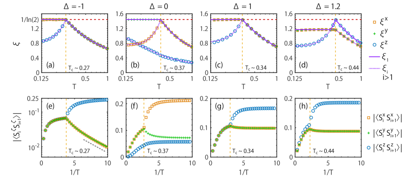
Fig. 7(a-d) shows the correlation lengths obtained with the above two approaches. The correlation length determined from the dominating correlators, for and for , exhibits cusps exactly at the critical temperatures . The value of the correlation length at the critical point, , equals the critical upper bound of the correlation length on the Bethe lattice. As discussed in Ref. Li et al., 2012, the number of spins that correlate with a root spin at a given site grows exponentially with their distances. Therefore, a magnetic order-disorder phase transition with a diverging magnetic susceptibility happens when , though being finite, reaches the critical value .
For the cases shown in Fig. 7(a,c), the correlation lengths, along all three directions, are all equal to the dominant correlation length in the paramagnetic phase above . Below , the transverse excitation modes remain critical and do not change with temperature, i.e., the corresponding correlation lengths still equal the dominant one, . Moreover, the longitudinal drops immediately below with decreasing temperature, due to the formation of magnetic order along the -direction. Similar critical behavior has been observed in Fig. 7(b) with , where the degeneracy between and is broken, since the ordering of spins happens along the -direction.
For the case in Fig. 7(d), is still the dominant correlation length above , which reaches the critical value and drops below . On the other hand, never reaches the critical value , although they do not decay below , and surpasses at a temperature below .
The peculiar behaviors of the transverse correlation lengths observed in the ordered phases are quite remarkable. It indicates that although the true Goldstone modes are absent in the continuous symmetry breaking phases Laumann et al. (2009), the transverse excitations remain “critical” with a maximal correlation length on the Bethe lattice. These quasi-critical transverse excitation modes are reminiscent of the Goldstone modes in a truly gapless continuous-symmetry-breaking system, and they can be regarded as somewhat “renormalized” Goldstone modes.
Distinct from the true gapless modes, and as the finite correlation lengths imply, these quasi-Goldstone modes are always gapped, and they become activated only above certain finite energy scales/temperatures, giving rise to the finite- phase transitions. Note that such kind of quasi-Goldstone modes are absent in the -symmetry-breaking phase, again similar to the two-dimensional lattices where Goldstone modes are absent for .
As a complementary to correlation length data, we show in Figs. 7(e-h) the absolute value of NN correlators (). In Fig. 7(e,g), we see distinct behaviors of NN correlators between the FM () and AF () cases. In the AF phase, approaches a finite value in the zero temperature limit. However, in the FM case, decays exponentially as decreases and it approaches zero in the limit. This is consistent with the fact that the FM ground state is simply a direct-product state , while the AF ground state bears quantum entanglement. Moreover, as shown in Figs. 7(f,h), and are strongest NN correlators in the and cases, respectively. In addition, other spin correlators in these two cases converge to finite values in the limit.
IV Linear Spin Wave Theory
Here we provide a linear spin wave analysis of the XXZ model on the Bethe lattice. The results reveal more information on the low-lying excitations, especially on the quasi-Goldstone mode in the continuous symmetry breaking phase.
IV.1 The ferromagnetic Heisenberg model
We first consider the excitations in the FM phase with . By taking a U(1) rotation for all the spins on the sublattice, we can transform Eq. (1) into the form
| (17) |
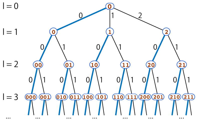
To carry out the linear spin-wave expansion, we choose an arbitrary site as a “root”, labelled as , and then there exists an unique path that connects it to any other lattice site, rendering a convenient way to label the Bethe lattice sites. More specifically, we label the lattice according to the rule shown in Fig. 8: a site in the -th layer from the root is represented by indices , where () denotes the way a path can choose at the -th branching point. On a -coordinated Bethe lattice, for the layer and for the rest layers.
Assuming all spins are up polarized in the ground state, we exploit the Holstein-Primakoff (HP) transformation and take the leading approximation for the spin operators, , and , where , are boson annihilation and creation operators, respectively. Under the linear spin-wave approximation, the Hamiltonian becomes
| (18) |
where is the particle number operator, and a constant energy term is dropped for the sake of simplicity.
To diagonalize the Hamiltonian (18), we first take the following multidimensional discrete Fourier transformation
| (19) |
where are the “quasi-momenta” which are dual to , and is a unitary matrix
| (20) |
Through this transformation, we generate a Bethe lattice with exactly the same geometry in the -space, i.e., .
Under the above transformation, the hopping term in Eq. (18) becomes
| (21) |
where denotes a site on the -th shell, next to site and with . On the other hand, the occupation number term remains as a number operator in the -space
| (22) |
More details of the transformation can be found in App. C.
Equation (21) with its hermitian conjugate implies that a boson on the site can only hop to site , and vice versa. indicate a site on -th shell, which is on the same branch of and further has . Therefore, for any given site with , there exists a one-dimensional path, consisting of , , , , etc.
The Hamiltonian on this half-infinite one-dimensional chain is tridiagonal, i.e.,
| (23) |
where , and is the starting node from which the one-dimensional path, depicted by a thick line in Fig. 8, is defined.
Secondly, we solve the above chain Hamiltonian via a conventional Fourier transformation, and the spin wave energy spectrum is found to be
| (24) |
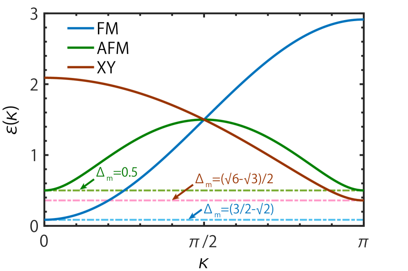
where is the momentum along the “effective” chains on the -space Bethe lattice. From Eq. (24), as well as the plot in Fig. 9, we find the magnon excitation energy gap as
| (25) |
The single magnon state is an eigenstate of the original Heisenberg FM model, and thus the magnon gap obtained in Eq. (25) constitutes an upper bound of the true excitation gap of the system. Matter of fact, as shown in Tab. 1, the energy gap obtained with this equation, , is very close to the value estimated from the TTN calculation. In addition, from Eq. (25) one can see clearly that increases linearly with , in excellent consistency with the TTN results (see also Tab. 1).
From the above discussion, we notice that each branch of magnon excitations is confined to a one-dimensional path which is formed by a symmetrized () superposition of real-space sites. This symmetry has already been exploited in some previous works Brinkman and Rice (1970); Lepetit et al. (1999); Mahan (2001); Petrova and Moessner (2016), however, the - transformation we introduce here works in a more generic way.
IV.2 Antiferromagnetic Heisenberg model
For the AF model with , the linear spin wave expansion can be similarly done by explicitly considering the spin orientations on the two sublattices. We start from the configuration that all the spins are upward aligned on the -sublattice and downward aligned on the -sublattice. Accordingly, we take a two-sublattice HP transformation, i.e., , and , for , and , and for . Therefore, the Hamiltonian under the linear spin wave approximation can be written as
| (26) |
A constant term is again omitted in obtaining the above expression.
To cope with the two-sublattice structure, we need to adopt different transformations on diffferent sublattices, namely taking on the -sublattice and on the -sublattice. Under this transformation, the pair annihilation term becomes (App. C)
| (27) |
The above Hamiltonian can then be effectively represented as a direct sum of the infinite-many one-dimensional models defined by the model
| (28) |
Employing the standard Bogoliubov transformation, the energy spectrum of is found to be (and plotted in Fig. 9)
| (29) |
The energy gap is, , for . Since the single-magnon excitation state is not an eigenstate of the original AF model, may not be an upper bound of the true excitation gap. Nonetheless, from Tab. 1 we observe that still provides a quite good estimate of the magnon gap.
IV.3 The XY model
The magnon bands of FM and AF cases become unstable when (more precisely, when ). To perform a linear spin-wave analysis for the XY phase, we needs to start from a classical state in which the spins are ordered on the XY plane.
Below, for the sake of simplicity, we consider only the case . The Hamiltonian can be equivalently written as
| (30) |
Under the linear spin-wave approximation, it becomes
| (31) |
To solve this problem, we use the following - transformation matrix
| (32) |
This particular choice ensures to be a real orthogonal matrix with the property
From this, again we obtain an effective one-dimensional boson model
| (33) |
Diagonalizing this Hamiltonian using the Bogoliubov transformation (App. D), the magnon excitation energy is found to be (Fig. 9)
| (34) |
The excitation gap is , which is for and , close to the numerical results, , shown in Tab. 1.
V Summary
We have investigated the Heisenberg XXZ model using both the canonical TTN and linear spin-wave theory on the Bethe lattice. Through efficient and accurate tensor network simulations, we have obtained the finite-temperature phase diagram of the model. The system undergoes a second-order phase transition at finite temperature, and three kinds of magnetic ordered phases are uncovered in low . The correlation lengths, as well as bipartite entanglements, though exhibiting their maximal values at the transition temperature , are found to be always finite on the Bethe lattice. Correspondingly, the low-lying excitations are revealed, through both numerical TTN and analytical spin wave calculations, to be gapped, even in the parameter range where the system breaks spontaneously the continuous symmetries.
Therefore, although the conventional gapless Goldstone modes are absent, quasi-Goldstone transverse fluctuation modes have been observed in the Bethe lattice XXZ model. When the system spontaneously breaks the continuous symmetries, the transverse correlation lengths reach the “critical” value, , and remain there for . Here is the maximal correlation length that is allowed on the Bethe lattice.
The results obtained on the Bethe-like lattices can be used to understand physical properties of quantum lattice models on the honeycomb, square, or other regular lattices. In addition, the canonical TTN method we proposed works very generally, and it can be applied to other fundamental quantum many-body models, such as the frustrated Heisenberg and Hubbard models defined on the Bethe-like lattices, etc.
VI acknowledgements
This work was supported by the National Natural Science Foundation of China (11834014, 11888101), the National R&D Program of China (2017YFA0302900). WL is indebted to Andreas Weichselbaum for helpful discussions. DWQ and WL would like to thank Jan von Delft for hospitality during a visit to LMU Munich, where part of this work was performed.
Appendix A Tensor update on the Bethe lattice
A.1 Bethe lattice update
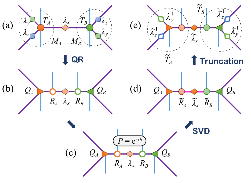
An imaginary time evolution can be employed to cool down the TTN density operator on the Bethe lattice, where the local tensors are updated via a simple scheme. The details are illustrated in Fig. A1 and elaborated below. We take the the -bond update as an example, and the successive projection procedures on the other two, i.e., - and -bonds, can be accomplished similarly. The three projection substeps on different bonds constitute a full Trotter step of small imaginary-time slice .
(a) Absorb the environment matrices and to the tensors and construct the tensor [Fig. A1(a)]
| (A1) |
where .
(b) Perform a QR decomposition of [Fig. A1(b)]
| (A2) |
which splits off the upper physical indices into the tensors.
(c) Construct a base tensor by combining with the two adjacent tensors and
| (A3) |
and apply the two-site imaginary-time evolution gate onto the base tensor [Fig. A1(c)]
| (A4) |
(d) Reshape into a matrix by grouping together with as a single index, and with into another. Then we perform a matrix SVD
| (A5) |
as shown in Fig. A1(d). Note that the matrix dimension of is enlarged by times after the bond evolution, which needs to be truncated by retaining only the largest singular values and corresponding bond bases. After this proper truncation of bond states, we update the tensors , and accordingly.
(e) Combine to the corresponding tensors, and spit off the matrices, that have been absorbed into in steps (a,b), by multiplying their inverse matrices to . Thus we obtain the updated tensors [Fig. A1(e)]
| (A6) |
where again denoting two sublattices.
In the groundstate optimization Li et al. (2012), the above procedure suffices to produce accurate results. The truncation errors do not accumulate, and can be tuned to a sufficiently small value, say, in the end of projections. However, in the finite-temperature simulations, now the truncation errors accumulate, we therefore need to carefully optimize the truncations in every single step to improve the overall performance. Note that () is not unitary and breaks the orthogonality of bond basis, and thus TTN deviates the canonical form after each step of imaginary-time evolution. Therefore, a canonicalization procedure of the TTN is needed to restore the orthogonality of bond bases and optimize the truncations.
A.2 Canonicalization procedure of TTN
Following a similar line of standard procedure developed in the matrix product Vidal (2007); Orús and Vidal (2008); Orús (2014) as well as tensor product states Ran et al. (2012), we present below the canonicalization of TTN on the Bethe lattice.
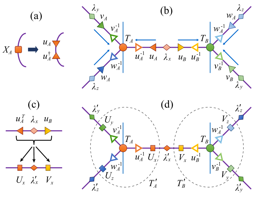
(i) As shown in Fig. A2(a), we decompose the dominant eigenvectors of the transfer tensors as
| (A7) |
where . Since in practice , and matrices are symmetric, the decomposition can be done via the eigenvalue or the Cholesky decomposition.
(ii) Insert pairs of reciprocal matrices, , and , to the three geometrical bonds, as shown in Fig. A2(b). Order of the matrix multiplication has also been specified by the arrows, e.g., we contract the first index of with and the second index of with .
(iii) Now we perform the bond update by combining the bond matrices and then perform a SVD. As shown in Fig. A2(c), we take the -bond as an example, i.e.,
| (A8) |
and are unitary matrices, and is used to update the bond diagonal matrix.
(iv) As shown in Fig. A2(d), we absorb , and matrices, as well as the adjacent unitary matrices and , into the tensors, and update and .
After the above procedure on the bond (and simultaneously on the and bonds), the updated tensors satisfy the canonical conditions [see Eq. (2) of the main text], and the dominating eigenvectors are now gauged into identities.
A.3 Simple vs. canonical schemes
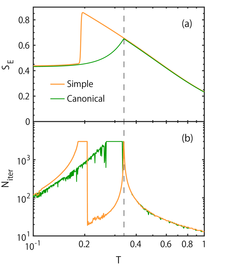
Now we provide some numerical benchmarks of the simple and canonical update schemes, showing the advantage of the latter in both the accuracy and robustness. Here by canonical scheme we mean the combined procedure using techniques introduced in both Secs. A.1 and A.2; while by simple scheme we mean a poorman’s approach where the canonicalization operations in Sec. A.2 are skipped.
We consider the Heisenberg model (), and compare the entanglement entropy and the number of iterations required to reach a convergence in determining the dominant eigenvectors in Eq. (8) of the main text. Although the entanglement entropy defined in Eq. (11) is rigorously defined only for canonical TTN, we can nevertheless take “” from the simple scheme as a measurement of entanglement for comparisons.
As seen in Fig. A3(a), the two curves almost coincide for . However, their behaviors start to differ at the critical temperature . The curve of the canonical scheme shows a cusp at the critical temperature and slowly converges to a smaller zero-temperature entanglement value, while that of the simple scheme still rises smoothly until collapsing at certain lower temperature below . After this “jump”, the simple scheme curve lies almost on top of the canonical curve, and both converge to the entanglement value in nearly the same rate.
Correspondingly, as shown in Fig. A3(b), peaks at in the canonical scheme, and it peaks both at and the “jump” point at a lower in the simple scheme curve. The second peak in in the simple scheme belongs to an numerical “artifact”, since no phase transition really takes place there.
Apart from the “artifact” in , the more severely accumulated errors in the simple scheme, as the temperature lows down, may cause other problems. In practice, sometimes the simple scheme is found to generate “wrong” metastable thermodynamic results, e.g, magnetic moments, at low temperatures .
To conclude, the canonical scheme turns out to be more accurate and robust, and it is thus mostly adopted in our practical simulations.
Appendix B Classical Ising model on the Bethe lattice
In this appendix, we provide the rigorous solution of the classical Ising model on the Bethe lattice via transfer tensor techniques. The TTN algorithms introduced in Sec. II can also be employed to compute this classical model, and the comparisons between the numerical and rigorous results thus provide a first benchmark of the TTN algorithm.
The Hamiltonian (energy) of the classical Ising model reads , where is the energy scale, means NN sites on the Bethe lattice, and denotes the classical Ising variables.
This Ising model can be solved exactly through a number of essentially equivalent methods, including the self-similarity Baxter (2013); Ostilli (2012) and cavity approaches Mézard and Parisi (2001); Ostilli (2012), etc. By solving the generalized eigenvalue problem, we find the dominant eigenvectors of the transfer tensor , from which we further obtain the exact expression of thermal quantities.
Firstly, we rewrite the partition function as a TTN, i.e.,
| (A9) |
where is a transfer tensor, and sits in the two central sites in the bond-centered [see, e.g., Fig. 1(b)]. The labelling in follows the convention shown in Fig. 8, but starts from 1 instead of 0 here.
Efficient contractions of this infinite TTN can be implemented by finding the dominant (generalized) eigenvectors of the transfer tensor , i.e.,
| (A10) |
with the (generalized) eigenvalue . By writing it down explicitly, we have
| (A11) |
Since Eq. (A11) does not constitute a linear system of equations, one has a gauge degrees of freedom in determining the eigenvalue as well as the eigenvector . Nevertheless, we can eliminate from the equations, and arrive at a cubic equation after some rearrangement,
| (A12) |
where . Note that the eigenvalue can now be expressed as , which can not be uniquely determined and depends on the normalization condition of (see related discussions in Sec. II.3).
The (unnormalized) probability distribution for two neighboring spin variables is . By summing over , we can get the distribution of a single spin , from which the magnetization can be derived as . Note that is just the root of Eq. (A12), and thus the local magnetization can be uniquely determined.
The order parameter, i.e., the spontaneous magnetization , reads
| (A13) |
with and the critical point .
Apparently, the root (and thus ) corresponds to the paramagnetic solution, while the two roots of the remaining quadratic equation in Eq. (A12) reflects the two-fold degenerate FM states. The sign represents the spin-up and spin-down solutions, respectively, given that the discriminant , i.e., .
The internal energy per bond can be determined from , which is
| (A14) |
It is clear that the curve exhibits a singular point at the transition temperature .
On the other hand, the Bethe-lattice Ising model can also be solved by the TTN techniques. By performing a decomposition following Eq. (3), and then an imaginary-time evolution procedure, we obtain the thermal density matrix of the classical Ising model on the Bethe lattice. On top of that, we can further calculate the thermal quantities, including the magnetization, energy, and specific heat, etc.
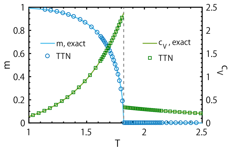
In Fig. A4, we compare the TTN results of the spontaneous magnetization and the specific heat to the exact solution, where excellent agreements can be observed. This can be ascribed to the absence of Trotter errors in the calculations, and also to no essential truncations in the procedure of cooling.
It is also of interest to note, in Eq. (A13), that the spontaneous magnetization with , when approaches the transition temperature (from low temperature side). In addition, the internal energy curve is continuous at , while the slope shows a discontinuity in Fig. A4(b), suggesting a mean-field-type critical exponent .
Appendix C The - transformation
Here we provide more details on the - transformations of the bilinear terms, including the hopping, on-site occupation number, pair-creation or annihilation terms, etc.
Firstly, we check that the real-space on-site term remains as on-site term in the -space
| (A15) |
For the NN hopping term, we have
| (A16) |
where for layers and for one.
In the HAF model, we have pair-creation and annihilation operators, where additional care needs to be taken of, i.e.,
| (A17) |
Therefore, the pair creation and annihilation operators can be transformed into -space in a well organised way, e.g.,
| (A18) |
which again falls into an effective 1D chain geometry.
Appendix D The Bogoliubov transformation in the XY model
In this appendix, we provide the details of the Bogoliubov transformation for the XY model. We start from the 1D half-chain bosonic Hamiltonian, i.e., Eq. (33) in the main text. By ignoring the “impurity site” at the center, performing a Fourier transformation on an infinite chain (without changing the energy dispersion curve), we arrive at , where
| (A19) |
with .
The sub-Hamiltonian can be rewritten as , where , and
| (A20) |
where we have omitted the term which is a constant after summing over .
In the Bogoliubov transformation, we find a matrix so that (1) , where still represents boson operators obeying the bosonic statistics, and (2) is in a diagonal form.
To maintain the boson statistics in condition (1), we require , where
and is a identity matrix.
Combing together conditions (1) and (2), we have , which implies and can be found by diagonalizing . After some calculations, and by observing that the Hamiltonian matrix in Eq. (A20) is block diagonal, we arrive at
where the positive root with constitutes the magnon spectrum in Eq. (34), i.e., . The corresponding Bogolon (annihilation) operator turns out to be
| (A21) |
with restriction , where can be determined from .
References
- Bethe (1935) H. A. Bethe, “Statistical theory of superlattices,” Proc. R. Soc. A 150, 552 (1935).
- Pathria and Beale (2011) R. K. Pathria and P. D. Beale, Statistical Mechanics (Academic Press; 3 edition, 2011).
- Ostilli (2012) M. Ostilli, “Cayley trees and Bethe lattices: A concise analysis for mathematicians and physicists,” Physica A 391, 3417 (2012).
- Eckstein et al. (2005) M. Eckstein, M. Kollar, K. Byczuk, and D. Vollhardt, “Hopping on the Bethe lattice: Exact results for densities of states and dynamical mean-field theory,” Phys. Rev. B 71, 235119 (2005).
- Petrova and Moessner (2016) O. Petrova and R. Moessner, “Coulomb potential problem on the bethe lattice,” Phys. Rev. E 93, 012115 (2016).
- Semerjian et al. (2009) G. Semerjian, M. Tarzia, and F. Zamponi, “Exact solution of the Bose-Hubbard model on the Bethe lattice,” Phys. Rev. B 80, 014524 (2009).
- Jiang et al. (2008) H. C. Jiang, Z. Y. Weng, and T. Xiang, “Accurate determination of tensor network state of quantum lattice models in two dimensions,” Phys. Rev. Lett. 101, 090603 (2008).
- Verstraete et al. (2008) F. Verstraete, V. Murg, and J. I. Cirac, “Matrix product states, projected entangled pair states, and variational renormalization group methods for quantum spin systems,” Adv. Phys. 57, 143 (2008).
- Orús (2014) R. Orús, “A practical introduction to tensor networks: Matrix product states and projected entangled pair states,” Ann. Phys. 349, 117 (2014).
- Li et al. (2012) W. Li, J. von Delft, and T. Xiang, “Efficient simulation of infinite tree tensor network states on the Bethe lattice,” Phys. Rev. B 86, 195137 (2012).
- Li et al. (2010) W. Li, S.-S. Gong, Y. Zhao, and G. Su, “Quantum phase transition, universality class, and phase diagram of the spin- Heisenberg antiferromagnet on a distorted honeycomb lattice: A tensor renormalization-group study,” Phys. Rev. B 81, 184427 (2010).
- Liu et al. (2014) T. Liu, S.-J. Ran, W. Li, X. Yan, Y. Zhao, and G. Su, “Featureless quantum spin liquid, -magnetization plateau state, and exotic thermodynamic properties of the spin- frustrated Heisenberg antiferromagnet on an infinite husimi lattice,” Phys. Rev. B 89, 054426 (2014).
- Liu et al. (2015) T. Liu, W. Li, A. Weichselbaum, J. von Delft, and G. Su, “Simplex valence-bond crystal in the spin-1 kagome Heisenberg antiferromagnet,” Phys. Rev. B 91, 060403 (2015).
- Liu et al. (2016) T. Liu, W. Li, and G. Su, “Spin-ordered ground state and thermodynamic behaviors of the spin- kagome Heisenberg antiferromagnet,” Phys. Rev. E 94, 032114 (2016).
- Otsuka (1996) H. Otsuka, “Density-matrix renormalization-group study of the spin-1/2 antiferromagnet on the Bethe lattice,” Phys. Rev. B 53, 14004 (1996).
- Friedman (1997) B. Friedman, “A density matrix renormalization group approach to interacting quantum systems on Cayley trees,” J. Phys.: Condens. Matter 9, 9021 (1997).
- Kumar et al. (2012) M. Kumar, S. Ramasesha, and Z. G. Soos, “Density matrix renormalization group algorithm for bethe lattices of spin- or spin-1 sites with Heisenberg antiferromagnetic exchange,” Phys. Rev. B 85, 134415 (2012).
- Changlani et al. (2013a) H. J. Changlani, S. Ghosh, C. L. Henley, and A. M. Läuchli, “Heisenberg antiferromagnet on cayley trees: Low-energy spectrum and even/odd site imbalance,” Phys. Rev. B 87, 085107 (2013a).
- Changlani et al. (2013b) H. J. Changlani, S. Ghosh, S. Pujari, and C. L. Henley, “Emergent spin excitations in a Bethe lattice at percolation,” Phys. Rev. Lett. 111, 157201 (2013b).
- Brinkman and Rice (1970) W. F. Brinkman and T. M. Rice, “Single-particle excitations in magnetic insulators,” Phys. Rev. B 2, 1324 (1970).
- Kittler and Falicov (1976) R. C. Kittler and L. M. Falicov, “Electronic structure of disordered binary alloys,” J. Phys. C: Solid State Phys. 9, 4259 (1976).
- Brouers and Marconi (1982) F. Brouers and U. M. B. Marconi, “On the antiferromagnetic phase in the Hubbard model,” J. Phys. C: Solid State Phys. 15, L925 (1982).
- Al Hajj et al. (2004) M. Al Hajj, N. Guihéry, J.-P. Malrieu, and P. Wind, “Theoretical studies of the phase transition in the anisotropic two-dimensional square spin lattice,” Phys. Rev. B 70, 094415 (2004).
- White (1992) S. R. White, “Density matrix formulation for quantum renormalization groups,” Phys. Rev. Lett. 69, 2863 (1992).
- Vidal (2007) G. Vidal, “Classical simulation of infinite-size quantum lattice systems in one spatial dimension,” Phys. Rev. Lett. 98, 070201 (2007).
- Orús and Vidal (2008) R. Orús and G. Vidal, “Infinite time-evolving block decimation algorithm beyond unitary evolution,” Phys. Rev. B 78, 155117 (2008).
- Li et al. (2011) W. Li, S.-J. Ran, S.-S. Gong, Y. Zhao, B. Xi, F. Ye, and G. Su, “Linearized tensor renormalization group algorithm for the calculation of thermodynamic properties of quantum lattice models,” Phys. Rev. Lett. 106, 127202 (2011).
- Dong et al. (2017) Y.-L. Dong, L. Chen, Y.-J. Liu, and W. Li, “Bilayer linearized tensor renormalization group approach for thermal tensor networks,” Phys. Rev. B 95, 144428 (2017).
- Ran et al. (2012) S.-J. Ran, W. Li, B. Xi, Z. Zhang, and G. Su, “Optimized decimation of tensor networks with super-orthogonalization for two-dimensional quantum lattice models,” Phys. Rev. B 86, 134429 (2012).
- Chen et al. (2017) B.-B. Chen, Y.-J. Liu, Z. Chen, and W. Li, “Series-expansion thermal tensor network approach for quantum lattice models,” Phys. Rev. B 95, 161104 (2017).
- Chen et al. (2018) B.-B. Chen, L. Chen, Z. Chen, W. Li, and A. Weichselbaum, “Exponential thermal tensor network approach for quantum lattice models,” Phys. Rev. X 8, 031082 (2018).
- Czarnik et al. (2012) P. Czarnik, L. Cincio, and J. Dziarmaga, “Projected entangled pair states at finite temperature: Imaginary time evolution with ancillas,” Phys. Rev. B 86, 245101 (2012).
- Czarnik and Dziarmaga (2015) P. Czarnik and J. Dziarmaga, “Variational approach to projected entangled pair states at finite temperature,” Phys. Rev. B 92, 035152 (2015).
- Czarnik et al. (2016) P. Czarnik, M. M. Rams, and J. Dziarmaga, “Variational tensor network renormalization in imaginary time: Benchmark results in the Hubbard model at finite temperature,” Phys. Rev. B 94, 235142 (2016).
- Czarnik et al. (2017) P. Czarnik, J. Dziarmaga, and A. M. Oleś, “Overcoming the sign problem at finite temperature: Quantum tensor network for the orbital model on an infinite square lattice,” Phys. Rev. B 96, 014420 (2017).
- Kshetrimayum et al. (2019) A. Kshetrimayum, M. Rizzi, J. Eisert, and R. Orús, “Tensor network annealing algorithm for two-dimensional thermal states,” Phys. Rev. Lett. 122, 070502 (2019).
- Czarnik et al. (2019) P. Czarnik, J. Dziarmaga, and P. Corboz, “Time evolution of an infinite projected entangled pair state: An efficient algorithm,” Phys. Rev. B 99, 035115 (2019).
- (38) P. Czarnik and P. Corboz, “Finite correlation length scaling with infinite projected entangled pair states at finite temperature,” arXiv:1904.02476 (2019) .
- Prosen and Pižorn (2007) T. Prosen and I. Pižorn, “Operator space entanglement entropy in a transverse Ising chain,” Phys. Rev. A 76, 032316 (2007).
- (40) T. Barthel, “One-dimensional quantum systems at finite temperatures can be simulated efficiently on classical computers,” arXiv:1708.09349 (2017) .
- (41) J. Dubail, “Entanglement scaling of operators: a conformal field theory approach, with a glimpse of simulability of long-time dynamics in 1 + 1d,” .
- Chen et al. (2019) L. Chen, D.-W. Qu, H. Li, B.-B. Chen, S.-S. Gong, J. von Delft, A. Weichselbaum, and W. Li, “Two-temperature scales in the triangular-lattice Heisenberg antiferromagnet,” Phys. Rev. B 99, 140404(R) (2019).
- Mermin and Wagner (1966) N. D. Mermin and H. Wagner, “Absence of ferromagnetism or antiferromagnetism in one- or two-dimensional isotropic Heisenberg models,” Phys. Rev. Lett. 17, 1133 (1966).
- Laumann et al. (2009) C. R. Laumann, S. A. Parameswaran, and S. L. Sondhi, “Absence of Goldstone bosons on the Bethe lattice,” Phys. Rev. B 80, 144415 (2009).
- Lepetit et al. (1999) M.-B. Lepetit, M. Cousy, and G. M. Pastor, “Density-matrix renormalization study of the Hubbard model on a Bethe lattice,” Eur. Phys. J. B 13, 421 (1999).
- Mahan (2001) G. D. Mahan, “Energy bands of the Bethe lattice,” Phys. Rev. B 63, 155110 (2001).
- Baxter (2013) R. J. Baxter, Exactly Solved Models in Statistical Mechanics (Courier Corporation, 2013).
- Mézard and Parisi (2001) M. Mézard and G. Parisi, “The Bethe lattice spin glass revisited,” Eur. Phys. J. B 20, 217 (2001).