Understanding the Effectiveness of Data Reduction in Public Transportation Networks

Abstract

Given a public transportation network of stations and connections, we want to find a minimum subset of stations such that each connection runs through a selected station. Although this problem is NP-hard in general, real-world instances are regularly solved almost completely by a set of simple reduction rules. To explain this behavior, we view transportation networks as hitting set instances and identify two characteristic properties, locality and heterogeneity. We then devise a randomized model to generate hitting set instances with adjustable properties. While the heterogeneity does influence the effectiveness of the reduction rules, the generated instances show that locality is the significant factor. Beyond that, we prove that the effectiveness of the reduction rules is independent of the underlying graph structure. Finally, we show that high locality is also prevalent in instances from other domains, facilitating a fast computation of minimum hitting sets.

1 Introduction

A public transportation network is a collection of stations along with a set of connections running through these stations. But beyond its literal definition, via bus stops and train lines, it also carries some of the geographical, social, and economical structure of the community it serves. Given such a network, we want to select as few stations as possible to cover all connections, i.e., each connection shall contain a selected station. This and similar covering problems arise from practical needs, e.g., when choosing stations for car maintenance, but their solutions also reveal some of the underlying structure of the network. Despite the fact that minimizing the number of selected stations is NP-hard, there is a surprisingly easy way to achieve just that on real-world instances: Weihe [19] showed for the German railroad network that two straightforward reduction rules simplify the network to a very small core which can then be solved by brute force. This is not a mere coincidence. Experiments have shown the same behavior on several other real-world transportation networks. Subsequently, the reduction rules became the standard preprocessing routine for many different covering problems. See the work of Niedermeier and Rossmanith [12], Abu-Khzam [1], or Davies and Bacchus [5], to name just a few. This raises the question as to why these rules are so effective. Answering this question would not only close the gap between theory and practice for the specific problem at hand, but also has the potential to lead to new insights into the networks’ structure and ultimately pave the way for algorithmic advances in bordering areas.

Our methodology for approaching this question is as follows. We first identify two characteristic properties of real-world transportation networks: heterogeneity and locality; see Section 2.2 for more details. Then we propose a model that generates random instances resembling real-world instances with respect to heterogeneity and locality. We validate our model by showing empirically that it provides a good predictor for the effectiveness of the reduction rules on real-world instances. Finally, we draw conclusions on why the reduction rules are so effective by running experiments on generated instances of varying heterogeneity and locality. Moreover, we show that our results extend beyond transportation networks to related problems in other domains.

For our model, we regard transportation networks as instances of the hitting set problem. From this perspective, connections are mere subsets of the universe of stations and we need to select one station from each set. Note that this disregards some of the structure inherent to transportation networks: A connection is not just a set of stops but a sequence visiting the stops in a particular order. In fact, the sequences formed by the connections are paths in an underlying graph, which itself has rich structural properties inherited from the geography. Focusing on these structural properties, we also consider the graph-theoretic perspective. The working hypothesis for this perspective is that the underlying graphs of real-world transportation networks have beneficial properties that render the instances tractable. We disprove this hypothesis by showing that the underlying graph is almost irrelevant. This validates the hitting set perspective, which disregards the underlying graph.

In Section 2, we formally state our findings on the graph-theoretic as well as the hitting set perspective. We study the hitting set instances of European transportation networks in Section 3, identifying heterogeneity and locality as characteristic features. In Section 4, we define and evaluate a model generating instances with these features. Section 5 extends our findings to other domains and Section 6 concludes this work.

2 Preliminary Considerations

Before discussing the results regarding the two different perspectives, we fix some notations and state the reduction rules introduced by Weihe [19]. A public transportation network (or simply a network) $N\,{=}\,(S,C)$ consists of a set $S$ of stations and a set $C$ of connections which are sequences of stations. That is, each connection $c\in C$ is a subset of $S$ together with a linear ordering of its elements. Two stations $s_{1},s_{2}\in S$ are connected in $N$ if there exists a sequence of stations starting with $s_{1}$ and ending in $s_{2}$ such that each pair of consecutive stations shares a connection. The subnetworks induced by this equivalence relation are called the connected components of $N$. Given $N\,{=}\,(S,C)$, the Station Cover problem is to find a subset $S^{\prime}\subseteq S$ of minimum cardinality such that each connection is covered, i.e., $S^{\prime}\cap c\not=\emptyset$ for every $c\in C$. The reduction rules by Weihe [19] are based on notions of dominance, both between stations and connections. For two different stations $s_{1},s_{2}\in S$, $s_{1}$ dominates $s_{2}$ if every connection containing $s_{2}$ also contains $s_{1}$. If so, there is always an optimal station cover without $s_{2}$, so it is never worse to select $s_{1}$ instead. Thus, removing $s_{2}$ from $S$ and from every connection in $C$ yields an equivalent instance. Similarly, for two different connections $c_{1},c_{2}\in C$, $c_{1}$ dominates $c_{2}$ if $c_{1}\subseteq c_{2}$. Every subset of $S$ covering $c_{1}$ then also covers $c_{2}$. Removing $c_{2}$ does not destroy any optimal solutions. Weihe’s algorithm can thus be summarized as follows. Iteratively remove dominated stations and connections until this is no longer possible. The remaining instance, the core, is solved using brute force. Each connected component can be solved independently and the running time is exponential only in the number of stations. Thus, the complexity of an instance denotes the maximum number of stations in any of its connected components.

The proofs of this section are in Appendix 0.A.

2.1 Graph-Theoretic Perspective

One way to represent a network $N=(S,C)$ is via an undirected graph $G_{N}$ defined as follows. The stations $S$ are the vertices of $G_{N}$; for each connection $(s_{1},\dots,s_{k})\in C$, $G_{N}$ contains the edges $\{s_{i},s_{i+1}\}_{1\leq i<k}$. The basic hypothesis of the graph-theoretic perspective is that certain properties of $G_{N}$ make the real-world Station Cover instances easy.

Consider a leaf $u$ in $G_{N}$, i.e., a degree-1 vertex. If there is a connection that contains only $u$, then this dominates all other connections containing $u$. Otherwise, all connections that contain $u$ also contain its unique neighbor. Thus, $u$ is dominated and removed by the reduction rules. We obtain the following proposition. The 2-core is the subgraph obtained by iteratively removing leaves [15].

Proposition 1

The reduction rules reduce any Station Cover instance $N$ to an equivalent instance $N^{\prime}$ such that $G_{N^{\prime}}$ is a subgraph of the 2-core of $G_{N}$, with additional isolated vertices.

Proposition 1 identifies the number of vertices in the $2$-core of $G_{N}$ as an upper bound for the core complexity. The following theorem shows that this bound is arbitrarily bad. Supporting this assessment, we will see in Section 3 that the $2$-cores of the graphs of real-world instances are rather large, while their core complexity is significantly smaller.

Theorem 2.1

For every graph $G$, there exist two Station Cover instances $N_{1}$ and $N_{2}$ with $G=G_{N_{1}}=G_{N_{2}}$ such that the core of $N_{1}$ has complexity $1$ while the core of $N_{2}$ corresponds to the $2$-core of $G$.

Theorem 2.1 disproves the working hypothesis of the graph-theoretic perspective. For any connected graph that has no leaves, there is a Station Cover instance that is completely solved by the reduction rules, and another instance on the very same graph that is not reduced at all. Furthermore, unless the $2$-core is small, the theorem shows that it is impossible to tell whether or not the reduction rules are effective on a given instance by only looking at the graph.

So far, we have only focused on Weihe’s algorithm. While our main goal is to explain the performance of this algorithm, one could argue that other methods exploiting different graph-theoretic properties are better suited to solve real-world instances. The next theorem, however, indicates that this is not the case. Even on “tree-like” graph classes Station Cover remains NP-hard. The reduction used to prove this theorem was originally given by Jansen [8].

Theorem 2.2 ([8], Theorem 5)

Station Cover is NP-hard even if the corresponding graph has treewidth 3 or feedback vertex number 2.

2.2 Hitting Set Perspective

Another way to represent a network $N$ is by an instance of the Hitting Set problem. Here, the connections $C\subseteq 2^{S}$ are regarded only as sets of stations (ignoring their order). An optimal cover is a minimum-cardinality subset of $S$ that has a non-empty intersection with all members of $C$. This perspective turns out to be much more fruitful. In the next section, we analyze the Hitting Set instances stemming from $12$ real-world networks. To summarize our results, we observe that the instances are heterogeneous, i.e., the number of connections containing a given station varies heavily. Moreover, the instances exhibit a certain locality, which probably has its origin in the stations’ geographic positions.

In more detail, for a station $s\in S$, let the number of connections in $C$ that contain $s$ be the degree of $s$. Conversely, for $c\in C$, $|c|$ is its degree. The connection degrees of the real-world instances are rather homogeneous, i.e., every connection has roughly the same size. Although there are different types of connections they appear to have a similar number of stops. The station degrees, on the other hand, vary strongly. In fact, we observe that the station degree distributions roughly follow a power law. This is in line with observations that, e.g., the sizes of cities are power-law distributed [6]. To quantify the locality of an instance, we use a variant of the so-called bipartite clustering coefficient [14].

We conjecture that heterogeneity of stations and locality of the network are the crucial factors that make the reduction so effective. If the station degrees vary strongly, chances are that some high-degree station exists that dominates many low-degree ones. Moreover, if locality is high, there tend to be several connections differing only in few stations and stations appearing in similar sets of connections. This increases the likelihood of dominance among the elements of both $S$ and $C$. To verify this hypothesis empirically, we propose a model for generating instances of varying heterogeneity and locality. Our findings suggest that higher heterogeneity decreases the core complexity, but the deciding factor is the locality. Finally, we observe that locality is also prevalent in other domains. As predicted by our model, preprocessing also greatly reduces these instances.

3 Analysis of Real-World Networks

Data Set	$|S|$	$\tfrac{|S|}{|C|}$	$\delta_{S}$	$\beta$	KS	$\kappa$	$2$-core	core
sncf	$1742\text{\,}$	$4.0$	$2.2$	$3.3$	$0.03$	$0.47$	70%	0.3%
nl	$4558\text{\,}$	$13.2$	$1.5$	$3.8$	$0.04$	$0.40$	70%	2.8%
kvv	$2115\text{\,}$	$8.0$	$2.1$	$3.5$	$0.03$	$0.48$	72%	0.8%
vrs	$5491\text{\,}$	$10.7$	$1.9$	$3.5$	$0.03$	$0.27$	83%	0.1%
rnv	$705\text{\,}$	$12.4$	$1.4$	$4.2$	$0.06$	$0.38$	54%	0.1%
athens	$5729\text{\,}$	$24.4$	$1.8$	$3.9$	$0.04$	$0.30$	89%	4.7%
petersburg	$4264\text{\,}$	$6.5$	$2.5$	$4.0$	$0.03$	$0.31$	86%	8.3%
warsaw	$3944\text{\,}$	$13.0$	$1.8$	$5.9$	$0.05$	$0.29$	80%	5.9%
luxembourg	$2484\text{\,}$	$7.3$	$2.7$	$2.9$	$0.02$	$0.25$	84%	0.2%
switzerland	$22\,535\text{\,}$	$5.6$	$2.0$	$4.5$	$0.02$	$0.33$	71%	1.7%
vbb	$3031\text{\,}$	$16.5$	$1.4$	$12.4$	$0.05$	$0.38$	73%	1.8%
db	$514\text{\,}$	$0.9$	$15.7$	$2.0$	$0.07$	$0.28$	78%	0.2%

Table 1: Transportation networks with atypical instances separated. Shown are the number $|S|$ of stations, the station-connection ratio $|S|/|C|$, average station degree $\delta_{S}$, estimated power-law exponent $\beta$, corresponding KS distance, bipartite clustering coefficient $\kappa$, relative $2$-core size, and the relative core complexity.

We examined several public transportation networks from different cities (athens, petersburg, warsaw), rural areas (sncf, kvv, vrs, rnv, vbb), and countries (nl, luxembourg, switzerland, db). The networks are taken from the transitfeeds.com repository. The raw data has the General Transit Feed Specification (GTFS) format. It stores multiple connections for the same route, one for each time a train actually drives that route. For each route, only one connection was used. Table 1 gives an overview of the relevant features of the resulting networks.

We reduced each instance to its largest component. For most of them, only a small fraction of stations and connections are disconnected from this component. A notable exception is the vbb-instance, representing the public transportation network of the city of Berlin, Germany. In total, it has $13\,424\text{\,}$ stations while its largest component has only $3031\text{\,}$. The reason is that different modes of transport are separated in the raw data. As a result, vbb has rather uncommon features. Another unusual case is the db-instance of the German railway network. Table 1 shows that most instances have a station-connection ratio $|S|/|C|$ of roughly $10$. For db, however, this ratio is at $0.9$ much smaller.

Heterogeneity.

The average station degree $\delta_{S}$ of the investigated networks is a small constant around $2$, independent of the instances’ complexity. The only exception is the db-network. This can be explained by the atypical value for $|S|/|C|$, and that each station is contained in much more connections. The average connection degree $\delta_{C}=\delta_{S}\cdot|S|/|C|$ (not explicitly given in the table) is roughly $20$, due to the station-connection ratios all being of the same order.

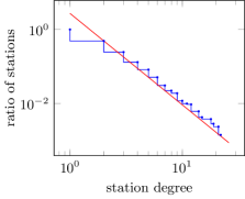
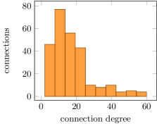
Figure 1: (left) The blue line is the CCDF of station degrees for the data set kvv. The red line is the estimated power-law distribution. (right) The histogram of connection degrees for the data set kvv.

Beyond small average degree, almost all instances exhibit strong heterogeneity among the degrees of different stations. We take a closer look at the kvv-instance as a prototypical example, representing the public transportation network of Karlsruhe, Germany. Figure 1 (left) shows the complementary cumulative distribution function (CCDF) of the station degrees in a log-log plot. For a given value $x$, the CCDF describes the share of stations that have degree at least $x$. The CCDF closely resembles a straight line (in log-log scaling), indicating a power-law distribution. That means, there exists a real number $\beta$, the power-law exponent, such that the number of stations of degree $x$ is roughly proportional to $x^{-\beta}$. We estimated the power-law exponents using the python package powerlaw [2]. For kvv, the exponent $\beta$ is approximately $3.5$. The goodness of fit is measured by the Kolmogorov–Smirnov distance (KS distance), which is the maximum absolute difference between the CCDFs of the measurement and of the assumed distribution. The KS distance for the kvv is $0.05$. Table 1 reports both the power-law exponents and the corresponding KS distances. The estimated values of $\beta$, excluding the outlier vbb, indicate a high level of heterogeneity. As a side note, the power-law exponent for vbb is $4.1$ with a KS distance of $0.03$ when considering the whole network instead of the largest component. In contrast, the connection degrees are rather homogeneous, cf. e.g. kvv in Figure 1 (right). A possible explanation is that long-distance trains stop less frequently.

Locality.

To measure locality, we adapt the bipartite clustering coefficient [14]. Intuitively, it states how likely it is that two stations which share a connection are also contained together in a different connection, or that two connections containing the same station also have another station in common. For a formal definition, first note that we can interpret a Hitting Set instance $(S,C)$ as a bipartite graph with the two partitions $S$ and $C$ and an edge joining $s\in S$ and $c\in C$ iff $s\in c$. Let $\#_{\mathrm{P}_{3}}$ denote the number of paths of length $3$ and $\#_{\mathrm{C}_{4}}$ the number of cycles of length $4$ in this graph. The bipartite clustering coefficient $\kappa$ then is defined as $\kappa=4\,{\cdot}\,\#_{C_{4}}/\#_{\mathrm{P}_{3}}$. It is the probability that a uniformly chosen $3$-path is contained in a $4$-cycle. Before computing $\kappa$, we normalize the bipartite graph by reducing it to its 2-core, which removes any attached trees. In doing so, the measure becomes more robust for our purpose, as attached trees do not impact the difficulty of an instance (they get removed by the reduction rules) while they decrease the clustering coefficient.

The clustering coefficients are reported in Table 1. All instances have a clustering coefficient of at least $0.25$, which indicates a high level of locality. A possible explanation are the underlying geographic positions of the stations, with nearby stations likely appearing in the same connection.

Degree of Reduction.

We measure the effectiveness of the reduction rules using the relative core complexity. It is the percentage of stations that remain after exhaustively applying the preprocessing. Table 1 shows that the resulting relative core complexity is very low for all 12 instances. This is in line with the original findings of Weihe [19], who applied the reduction rules on a few select European train networks. Moreover, it generalizes these results to networks of different scales, from urban to national. On the other hand, the $2$-core is typically not much smaller than the original instance. This shows that Proposition 1 cannot explain the effectiveness of the reduction rules, which supports our previous assessment that the graph-theoretic perspective is not sufficient.

Judging from Table 1, we believe that heterogeneity of the stations and high locality are the crucial properties rendering the preprocessing so effective. Notwithstanding, it is also worth noting that the reduction rules work well on all instances, including vbb which is not very heterogeneous. The clustering on the other hand is high for all instances, indicating that locality is more important. Also, the db and vbb outliers seem to show that the influence of the station-connection ratio and the average station degree is limited. Though looking at these $12$ networks can provide clues to what features are most important, it is not sufficient to draw a clear picture. In the following, we thoroughly test the effect of different properties on the effectiveness of the reduction rules by generating instances with varying properties.

4 Analysis of Generated Instances

This section discusses the generation and analysis of artificial Hitting Set instances. First, we present our model of generation which is based on the geometric inhomogeneous random graphs [4]. It allows creating networks with varying degree of heterogeneity and locality. We then analyze these instances with respect to the degree of reduction.

4.1 The Generative Model

In the field of network science, it is generally accepted that vertex degrees in realistic networks are heterogeneous [17]. A power-law distribution can be explained, inter alia, by the preferential attachment mechanism [3]. Beyond the generation of heterogeneous instances, different models have been proposed to also account for locality. The latter models typically use some kind of underlying geometry. One of the earliest works in that direction is by Watts and Strogatz [18]. More recently, and closer to our aim, Papadopoulos et al. [13] introduced the concept of popularity vs. similarity, making the creation of edges more likely, the more popular and similar the connected vertices are. They also observed that these two dimensions are naturally covered by the hyperbolic geometry, leading to hyperbolic random graphs [10]. Bringmann, Keusch, and Lengler [4] generalized this concept to geometric inhomogeneous random graphs (GIRGs). There, each vertex has a geometric position and a weight. Vertices are then connected by edges depending on their weights and distances. Despite a plethora of models for generating graphs, we are not aware of models generating heterogeneous Hitting Set instances. The closest is arguably the work by Giráldez-Cru and Levy [7], who generate SAT instances using the popularity vs. similarity paradigm.

To generate Hitting Set instances with varying heterogeneity and locality, we formulate a randomized model based on GIRGs. Each station and connection has a weight representing its importance. Moreover, stations and connections are randomly placed in a geometric space. The distance between stations and connections then provides a measure of similarity. In the Hitting Set instance, some station $s$ is a member of connection $c$ with a probability proportional to the combined weights of $s$ and $c$ and inverse proportional to the distance between the vertices $s$ and $c$. To make this more precise, let $w_{S}\colon S\to\mathbb{R}$ and $w_{C}\colon C\to\mathbb{R}$ be two weight functions; we omit the subscript when no ambiguity arises. For $s\in S$ and $c\in C$, let $\operatorname{dist}(s,c)$ denote the geometric distance between the corresponding vertices. Finally, fix two positive constants $a,T>0$. Then, station $s$ is contained in connection $c$ with probability

$$P(s,c)=\min\left\{1,\ \left(a\cdot\frac{w(s)w(c)}{\operatorname{dist}(s,c)}\right)^{1/T}\right\}.$$ (1)

The parameter $a$ governs the expected degree. The temperature $T$ controls the influence of the geometry. For $T\,{\to}\,0$ the method converges to a step model, where $s$ is contained in $c$ if and only if $\operatorname{dist}(s,c)\,{\leq}\,a\hskip 1.00006ptw(s)w(c)$. Larger temperatures soften this threshold, allowing $s\in c$ for larger distances, and $s\notin c$ for smaller distances, with a low probability. Thus, $T$ influences the locality of the instance.

The remaining degrees of freedom are the choice of the underlying geometry and the weights. For the geometry, we use the unit circle. Positions for stations and connections are drawn uniformly at random from $[0,1]$ and the distance between $x,y\in[0,1]$ is $\min\{|x\,{-}\,y|,1\,{-}\,|x\,{-}\,y|\}$. This is arguably the simplest possible symmetric geometry.

To choose the weights properly, it is important to note that the resulting degrees are expected to be proportional to the weights [4]. Thus, we mimic the real-world instances by choosing uniform weights for the connections and power-law weights, with varying exponent $\beta$, for the stations. It is not hard to see that for $\beta\to\infty$, the latter converge to uniform weights as well. In summary, adjusting $\beta$ controls the heterogeneity.

4.2 Evaluation

We generate artificial networks and measure the dependence of their relative core complexity on the heterogeneity and locality. The size of an instance has three components: the (original) complexity $|S|$, the station-connection ratio $|S|/|C|$, and the average station degree $\delta_{S}$. Note that these values also determine the number $|C|$ of connections and average connection degree $\delta_{C}$. From the model, we have the two parameters we are most interested in, the power-law exponent $\beta$ and the temperature $T$. We also consider the limit case of uniform weights for all vertices; slightly abusing notation, we denote this by $\beta=\infty$.

For the main part of the experiments, we used $|S|=$2000\text{\,}$$, $|S|/|C|=10.0$, and $\delta_{S}=2.0$, leaning on the respective properties for the real-world instances. We let $T$ vary between $0$ and $1$ in increments of $0.05$, and $\beta$ between $2$ and $5$ in increments of $0.25$. For each combination, we generated ten samples. In the following, we first validate the data. Then we examine the influence of heterogeneity and locality. Afterwards we test whether our findings still hold true for different station-connection ratios and station degrees.

Data Validation.

There are two aspects to the data validation. First, the instances should approximately exhibit the properties we explicitly put in, i.e., the values of $|S|$, $|S|/|C|$, $\delta_{S}$, and the power-law behavior. Second, the implicit properties should also be as expected. In our case, we have to verify that changing $T$ actually has the desired effect on the bipartite clustering coefficient $\kappa$.

Concerning the complexity $|S|$, note that a sampled instance per se does not need to be connected. If it is not, we again only use the largest component. Thus, when generating an instance with $2000\text{\,}$ stations, the resulting complexity is actually a bit smaller. There are typically many isolated stations due to the small average station degree, this is particularly true for small power-law exponents. However, the complexity of the largest component never dropped below $1000\text{\,}$ and usually was between $1400\text{\,}$ and $1700\text{\,}$ provided that $\beta>2.5$. The transition to the largest component mainly meant ignoring isolated stations. Thus, also the station-connection ratio $|S|/|C|$ decreases slightly. For $\beta>3$ it was typically around $8$ and always at least $7$. For smaller $\beta$, it is never below $5$.

Recall that the average station degree $\delta_{S}$ is controlled by parameter $a$ in Equation 1. It is a constant in the sense that it is independent of the considered station-connection pair. However, it does depend on other parameters of the model. As there is no closed formula to determine $a$ from $\delta_{S}$, we estimated it numerically. This estimation incurred some loss in accuracy but yielded values of $\delta_{S}$ between $1.9$ and $2.1$, very close to the desired $\delta_{S}=2$. Transitioning to the largest component typically slightly increases $\delta_{S}$, as the largest component is more likely to contain stations of higher degree. Anyway, $\delta_{S}$ never went above $2.7$.

As with the real-world instances, we estimated the exponent $\beta$ of the generated instances. For small values, the estimates matched the specified values. For larger exponents, the gap increases slightly, e.g., an estimated $\beta=5.7$ for an instance with predefined parameter $5.0$.

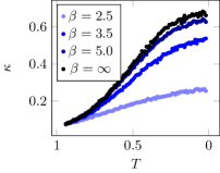
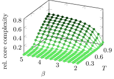
Figure 2: (left) The clustering coefficient $\kappa$ depending on the temperature $T$ for different $\beta$. (right) The relative core complexity depending on the power-law exponent $\beta$ and temperature $T$.

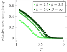
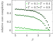
Figure 3: The relative core complexity (left) depending on the temperature $T$ (for different power-law exponents $\beta$), and (right) depending on $\beta$ (for different $T$).

Finally, we examined the dependency between the bipartite clustering coefficient $\kappa$ and the temperature $T$; see Figure 2 (left). As desired, the clustering coefficient increases with falling temperatures. More precisely, $\kappa$ ranges between $0$ and some maximum attained at $T=0$. The value of this maximum depends on the power-law exponent $\beta$, with smaller $\beta$ giving smaller maxima.

Heterogeneity and Locality.

For each instance described above, we computed the relative core complexity. To reduce noise, we look at the arithmetic mean of ten samples for each parameter configuration. The measured core complexities and clustering coefficients in fact showed only small variance, with almost all values differing at most $5\%$ from the respective mean. These measurements are presented in Figure 2 (right), showing the mean core complexity depending on the temperature $T$ and the power-law exponent $\beta$. For all parameter configurations, the relative core complexity was at most $50\%$. This is due to the low average station degree, which leads to dominant low-degree stations. More importantly, the core complexity varies strongly for different values of $T$ and $\beta$.

The complexity decreased both with lower temperatures and lower power-law exponents. This further supports our claim that heterogeneity and locality both have a positive impact on the effectiveness of the reduction rules. The locality, however, seems to be more vital. To make this precise, low temperatures lead to small cores, independent of $\beta$, as shown in Figure 3 (left). Even under uniform station weights ($\beta=\infty$), temperatures below $0.3$ consistently produced instances with empty core. In contrast, the power-law exponent has only a minor impact. One can see in Figure 3 (right) that for low temperatures, the core complexity is (almost) independent of $\beta$. For higher temperatures, the core complexities remain high over wide ranges of $\beta$, except for very low exponents.

In summary, high locality seems to be the most prominent feature that makes Station Cover instances tractable, independent of their heterogeneity. Heterogeneity alone reduces the core complexity only slightly, except for extreme cases (very low power-law exponents). It is thus not the crucial factor. In the following, we verify this general behavior also for alternative model parameters such as station-connection ratio or average station degree.

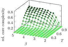
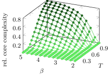
Figure 4: The relative core complexity depending on the power-law exponent $\beta$ and temperature $T$ under alternative model parameters. (left) The station-connection ratio is $|S|/|C|=4.0$ (instead of $10.0$). (right) The average station degree is $\delta_{S}=5.0$ (instead of $2.0$).

Station-Connection Ratio.

Recall that we fixed a ratio of $|S|/|C|=10.0$ for the main part of our experiments. To see whether our observations are still valid for different settings, we additionally generated data sets with mostly the same parameters as before, except for $|S|/|C|=4.0$. The result are shown in Figure 4 (left). Comparing this to Figure 2 (right), one can see that general dependence on $T$ and $\beta$ is very similar. However, there are subtle differences. Under the smaller station-connection ratio the instances are tractable even for larger temperatures, up to $T=0.5$ instead of the earlier $0.3$, i.e., for lower locality. Also, the maximum core complexity over all combinations of $T$ and $\beta$ is larger than before, reaching almost $60\%$, compared to the $50\%$ for $|S|/|C|=10.0$. In summary, in the (more realistic) low-temperature regime, a lower station-connection ratio seems to further improve the effectiveness of the reduction rules.

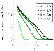
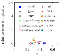
Figure 5: The relative core complexity depending on the clustering coefficient $\kappa$ (left) for generated instances with different values of the power-law exponent $\beta$, and (right) for the real-world instances.

Average Degree.

To examine the influence of the average station degree $\delta_{S}$, we generated another instance set with the same parameters as the main one, except that we increased the $\delta_{S}$ from $2.0$ to $5.0$. The results are shown in Figure 4 (right). Again the general behavior is similar, but now lower temperatures are necessary to render the instances tractable. Moreover, the maximum core complexity increases significantly, reaching up to almost $100\%$. Generally, a smaller average degree makes the reduction rules more effective. Intuitively speaking, the existence of stations with low degree increases the likelihood that the reduction rule of station dominance can be applied.

Comparison with Real-World Instances.

To compare generated and real-world instances more directly, we investigate the dependence between the relative core complexity and the bipartite clustering coefficient $\kappa$, instead of the model-specific temperature $T$. Figure 5 shows the results. Several of the real-world networks are well covered by the model. For example, our findings from the generated instances can be directly transferred to sncf and kvv. They have power-law exponents of $3.3$ and $3.5$, respectively, as well as clustering coefficients of at least $0.47$, which explains their small core complexity. Moreover, for luxembourg, the model can explain the low complexity in spite of a small clustering coefficient of $0.25$. The network exhibits a small exponent $\beta=2.9$, which benefits the effectiveness of the preprocessing. On the other hand, petersburg has clustering $\kappa=0.31$, but also a comparatively large core complexity of over $8\%$. Here, the main factor seems to be the high power-law exponent of $4.0$.

Notwithstanding, there are also some real-world instances that have an unexpectedly low core complexity, which cannot be fully explained by the model. The vrs-instance has a low clustering coefficient of $\kappa=0.27$ and a high power-law exponent of $3.5$, but still a very low $0.1\%$ core complexity. The reason seems to be its low average station degree of $\delta_{S}=1.9$. The switzerland-instance also has a low core complexity of $1.7\%$, despite its high power-law exponent of $\beta=4.5$ and a clustering coefficient of $\kappa=0.33$. Especially the high value of $\beta$ would point to a much higher complexity, however, its station-connection ratio $|S|/|C|=5.6$ is significantly lower than that of the generated instances. All in all, the networks generated by the model are not perfectly realistic. However, the model does replicate properties that are crucial for the effectiveness of the reduction rules on real-world instances. Furthermore, in the interplay of heterogeneity and locality, it reveals locality as the more important property.

5 Impact on Other Domains

Although the focus of this paper is to understand which structural properties of public transportation networks make Weihe’s reduction rules so effective, our findings go beyond that. Our experiments on the random model predict that Hitting Set instances in general can be solved efficiently if they exhibit high locality. Moreover, if the instance is highly heterogeneous, a smaller clustering coefficient suffices; see Figure 5 (left). The element-set ratio and the average degree have, within reasonable bounds, only a minor impact on the effectiveness. Our experiments in Section 4.2 showed that instances are more difficult for a larger average degree and if the difference between the number of elements and the number of sets is high. Experiments not reported in this paper show that the latter is also true, if there are more sets than elements (i.e., the ratio is below $1$).

Data Sets.

We consider Hitting Set instances from three different applications; see Table 2. The first set of instances are metabolic reaction networks of Escherichia coli bacteria. The elements represent reactions and each set is a so-called elementary mode. Analyzing the hitting sets of these instances has applications in drug discovery. The corresponding data sets, labeled ec-*, were generated with the Metatool [9]. In the second type of instance, the sets consist of so-called elementary pathways that need to be hit by interventions that suppress all signals, which is relevant, inter alia, for the treatment of cancer. The data sets, EGFR.* and HER2.*, were obtained via the OCSANA tool [16]. The instances country-cover and language-cover are based on a country-language graph, taken from the network collection KONECT [11], with an edge between a country and a language if the language is spoken in that country. The corresponding Hitting Set instances ask for a minimum number of countries to visit to hear all languages, and for a minimum number of languages necessary to communicate with someone in every country, respectively.

Data Set	$|S|$	$|S|/|C|$	$\kappa$	core
ec-acetate	$57\text{\,}$	0.214	$0.67$	1.8%
ec-succinate	$57\text{\,}$	0.061	$0.59$	1.8%
ec-glycerol	$60\text{\,}$	0.028	$0.66$	1.7%
ec-glucose	$58\text{\,}$	0.009	$0.66$	36.2%
ec-combined	$64\text{\,}$	0.002	$0.62$	40.6%
EGFR.short	$50\text{\,}$	0.400	$0.66$	2.0%
EGFR.sub	$56\text{\,}$	0.239	$0.57$	1.8%
HER2.short	$123\text{\,}$	0.230	$0.53$	9.8%
HER2.sub	$172\text{\,}$	0.068	$0.55$	10.4%
country-cover	$248\text{\,}$	0.407	$0.11$	0.4%
language-cover	$610\text{\,}$	2.460	$0.11$	0.2%

Table 2: Hitting Set instances from other domains. Listed are the number $|S|$ of elements, the element-set ratio $|S|/|C|$, the bipartite clustering coefficient $\kappa$, and the relative core complexity.

Evaluation.

The basic properties of the instances and the effectiveness of the reduction rules are reported in Table 2. The results match the prediction of our model: most instances have a high clustering coefficient and the reduction rules are very effective. The only instances that stand out at first glance are ec-glucose, ec-combined, HER2.short, and HER2.sub, which are not solved completely by the reduction rules despite their high clustering coefficients, as well as country-cover and language-cover, which are solved completely despite the comparatively low clustering coefficient of $\kappa=0.11$.

However, a more detailed consideration reveals that these instances also match the predictions of the model. First, the two instances country-cover and language-cover are very heterogeneous with power-law exponent $\beta=2.2$. As can be seen in Figure 2 (left), a clustering coefficient of $\kappa=0.11$ is already rather high for this exponent, leading to a low core complexity; see Figure 5 (left).

The instances ec-glucose and ec-combined have skewed element-set ratios (more than 100 times as many sets as elements) and a high average degree ($30\text{\,}$ for the sets; $\mathrm{3}\mathrm{k}$ and $\mathrm{1}\mathrm{3}\mathrm{k}$ for the elements, respectively). Thus, these instances at least qualitatively match the predictions of the model that the reduction rules are less effective if the element-set ratio is skewed or the average degree is high. One obtains a similar but less pronounced picture for HER2.short and HER2.sub.

6 Conclusion

We explored the effectiveness of data reduction for Station Cover on transportation networks. Our main finding is that real-world instances have high locality and heterogeneity, and that these properties make the reduction rules effective, with locality being the crucial factor. This directly transfers to general Hitting Set instances. For future work, it would be interesting to rigorously prove that the reduction rules perform well on the model.

Appendix 0.A Omitted Proofs

In this appendix, we sketch the omitted proofs of the theorems in Section 2.

Theorem 0.A.1

For every graph $G$, there exist Station Cover instances $N_{1}$ and $N_{2}$ with $G=G_{N_{1}}=G_{N_{2}}$ such that the core of $N_{1}$ has complexity $1$ while the core of $N_{2}$ corresponds to the $2$-core of $G$.

Proof (Proofsketch)

We assume that $G$ is connected, otherwise we apply the following to each component. For $N_{1}$, we choose connections such that there is a single designated station $s$ contained in each connection. Such connections can be constructed as follows. For an edge $\{u,v\}$ of $G$, construct a simple path that contains $s$ and the edge $\{u,v\}$. We use the stations on this path as a connection in $N_{1}$ and repeat this for every edge. It can be easily verified that $G_{N_{1}}=G$ and that the core of $N_{1}$ has complexity 1 ($s$ dominates all other stations).

For $N_{2}$, first assume that $G$ has no leaves, i.e., $G$ is already the $2$-core. It is then not hard to see that having one connection for each edge containing exactly its two endpoints prohibits any of the two reduction rules. In the general case, we have to be a bit more careful as applying reduction rules to leaves of $G$ can lead to connections that contain only a single station. These then lead to further reductions that can potentially cascade through the $2$-core. We prevent this as follows. For every edge in the $2$-core of $G$, we add the connection containing its two endpoints (as before). For every station $s$ not in the $2$-core, we find a simple path that contains $s$ and exactly one edge from the $2$-core. We add the connection containing the stations of this path to $N_{2}$. One can verify that indeed $G_{N_{2}}=G$ as every edge in $G$ corresponds to a pair of consecutive stations in at least one connection. Moreover, exhaustively applying the reduction rules leads to the $2$-core of $G$ with one connection for each edge.

Theorem 0.A.2 ([8], Theorem 5)

Station Cover is NP-hard even if the corresponding graph has treewidth 3 or feedback vertex number 2.

Proof (Proofsketch)

We prove this by reducing from 3-SAT. Let $\varphi$ be a propositional formula on $n$ variables. We create two vertices $x$ and $\overline{x}$ for every literal and connect them. Then, we add two vertices $z_{0}$ and $z_{1}$ which are connected to every $x$ vertex. For every literal, we add a path $(x,\overline{x})$. For every clause $(a\vee b\vee c)$ we add a path $(x_{a},z_{0},x_{b},z_{1},x_{c})$ where each $x_{i}$ is the vertex $\overline{x_{i}}$ or $x_{i}$ based on whether the variable is inverted or not. Figure 6 illustrates this reduction. Now, if and only if there is a path cover by vertices of size $n$ (where $n$ is the number of variables), the SAT instance is solvable. The graph created has a feedback vertex number of 2: if we remove both $z_{0}$ and $z_{1}$ from the graph, the only edges left are those between the vertices $x$ and $\overline{x}$ for each variable. The graph also has treewidth 3. Consider the following tree decomposition. For every variable $x$, we add a bag $\{x,\overline{x},z_{0},z_{1}\}$. Our tree decomposition now consists of all of these bags in one single path in an arbitrary order. Each vertex is in some bag. For every edge, there is a bag that contains both of its vertices. Finally, the only vertices that occur in multiple bags are $z_{0}$ and $z_{1}$, and since they are in every bag, this forms a subtree. Each bag has a size of 4, thus the graph has a treewidth of 3.

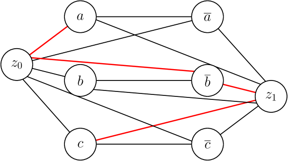
Figure 6: Illustration of the proof of Theorem 0.A.2. The resulting graph has treewidth 3. The path shown in red represents the clause $a\vee\overline{b}\vee c$.

References

- [1] Abu-Khzam, F.N.: A Kernelization Algorithm for -Hitting Set. Journal of Computer and System Sciences 76, 524–531 (2010)
- [2] Alstott, J., Bullmore, E., Plenz, D.: powerlaw: A Python Package for Analysis of Heavy-Tailed Distributions. PLOS One 9, e85777 (2014)
- [3] Barabási, A.L., Albert, R.: Emergence of Scaling in Random Networks. Science 286, 509–512 (1999)
- [4] Bringmann, K., Keusch, R., Lengler, J.: Sampling Geometric Inhomogeneous Random Graphs in Linear Time. In: Proceedings of the 25th Annual European Symposium on Algorithms (ESA). pp. 20:1–20:15 (2017)
- [5] Davies, J., Bacchus, F.: Solving MAXSAT by Solving a Sequence of Simpler SAT Instances. In: Proceedings of the 17th International Conference on Principles and Practice of Constraint Programming (CP). pp. 225–239 (2011)
- [6] Gabaix, X.: Zipf’s Law for Cities: an Explanation. The Quarterly Journal of Economics 114, 739–767 (1999)
- [7] Giráldez-Cru, J., Levy, J.: Locality in Random SAT Instances. In: Proceedings of the 26th International Joint Conference on Artificial Intelligence (IJCAI). pp. 638–644 (2017)
- [8] Jansen, B.M.P.: On Structural Parameterizations of Hitting Set: Hitting Paths in Graphs Using 2-SAT. Journal of Graph Algorithms and Applications 21, 219–243 (2017)
- [9] von Kamp, A., Schuster, S.: Metatool 5.0: Fast and Flexible Elementary Modes Analysis. Bioinformatics 22, 1930–1931 (2006)
- [10] Krioukov, D., Papadopoulos, F., Kitsak, M., Vahdat, A., Boguná, M.: Hyperbolic Geometry of Complex Networks. Physical Review E 82, 036106 (2010)
- [11] Kunegis, J.: KONECT - The Koblenz Network Collection. In: Proceedings of the 22nd International Conference on World Wide Web (WWW). pp. 1343–1350 (2013)
- [12] Niedermeier, R., Rossmanith, P.: An Efficient Fixed-Parameter Algorithm for 3-Hitting Set. Journal of Discrete Algorithms 1, 89–102 (2003)
- [13] Papadopoulos, F., Kitsak, M., Ángeles Serrano, M., Boguñá, M., Krioukov, D.: Popularity Versus Similarity in Growing Networks. Nature 489, 537–540 (2012)
- [14] Robins, G., Alexander, M.: Small Worlds Among Interlocking Directors: Network Structure and Distance in Bipartite Graphs. Computational & Mathematical Organization Theory 10, 69–94 (2004)
- [15] Seidman, S.B.: Network Structure and Minimum Degree. Social Networks 5, 269–287 (1983)
- [16] Vera-Licona, P., Bonnet, E., Barillot, E., Zinovyev, A.: OCSANA: Optimal Combinations of Interventions from Network Analysis. Bioinformatics 29, 1571–1573 (2013)
- [17] Voitalov, I., van der Hoorn, P., van der Hofstad, R., Krioukov, D.V.: Scale-free Networks Well Done. CoRR abs/1811.02071 (2018)
- [18] Watts, D.J., Strogatz, S.H.: Collective Dynamics of ‘Small-World’ Networks. Nature 393, 440–442 (1998)
- [19] Weihe, K.: Covering Trains by Stations or the Power of Data Reduction. In: Proceedings of the 1998 Algorithms and Experiments Conference (ALEX). pp. 1–8 (1998)