An assets-liabilities dynamical model of banking system and systemic risk governance

Abstract

We consider the problem of governing systemic risk in an assets-liabilities dynamical model of banking system. In the model considered each bank is represented by its assets and its liabilities. The capital reserves of a bank are the difference between assets and liabilities of the bank. A bank is solvent when its capital reserves are greater or equal to zero otherwise the bank is failed. The banking system dynamics is defined by an initial value problem for a system of stochastic differential equations whose independent variable is time and whose dependent variables are the assets and the liabilities of the banks. The banking system model presented generalizes those discussed in [4], [3] and describes a homogeneous population of banks. The main features of the model are a cooperation mechanism among banks and the possibility of the (direct) intervention of the monetary authority in the banking system dynamics. We call systemic risk or systemic event in a bounded time interval the fact that in that time interval at least a given fraction of the banks fails. The probability of systemic risk in a bounded time interval is evaluated using statistical simulation. The systemic risk governance pursues the goal of keeping the probability of systemic risk in a bounded time interval between two given thresholds. The monetary authority is responsible for the systemic risk governance. The governance consists in the choice of the assets and of the liabilities of a kind of “ideal bank” as functions of time and in the choice of the rules that regulate the cooperation mechanism among banks. These rules are obtained solving an optimal control problem for the pseudo mean field approximation of the banking system model. The governance induces the banks of the system to behave like the “ideal bank”. Shocks acting on the assets or on the liabilities of the banks are simulated. Numerical examples of systemic risk governance in presence and in absence of shocks acting on the banking system are studied.

1 Introduction

The notion of systemic risk refers to the risk of a collapse of an entire system rather than simply the failure of individual parts of it. Systemic risk and systemic risk governance are important research topics that have applications in many different contexts such as, for example, physics, biology, engineering, finance. We limit our attention to the modeling of systemic risk in banking systems. For a survey of the use of mathematical models in the study of systemic risk in a more general context we refer to [8] and to the references therein.

This paper is concerned with measurement, monitoring and governance of systemic risk in an assets-liabilities dynamical model of banking system. Recently several dynamical models of banking systems based on stochastic differential equations have been studied, see, for example, [4], [1], [6], [3]. We present a banking system model that generalizes those presented in [4], [3] and exploits some ideas taken from [7], [10], [11], [12]. That is we consider a continuous-time dynamical model of banking system where each bank holds assets and has liabilities that are stochastic processes of time. Assets and liabilities of each bank as functions of time are defined implicitly by an initial value problem for a system of stochastic differential equations. The capital reserves of a bank are defined as the difference between assets and liabilities of the bank. A bank is solvent when its capital reserves are greater or equal to zero otherwise the bank is failed. A political/technical authority is responsible for the banking system management and, in particular, is responsible for the systemic risk governance. For convenience we refer to this authority as monetary authority.

The model proposed describes a homogeneous population of banks where each bank interacts with the other banks and with the monetary authority. Note that the homogeneity of the bank population implies that all the banks of the model behave in the same way. The main features of the model are a cooperation mechanism among banks that regulates the inter-bank borrowing and lending activity and the possibility of the (direct) intervention of the monetary authority in the banking system dynamics. The cooperation mechanism among banks (see [4], [3]) is based on the idea that “who has more (assets, liabilities) gives to those who have less (assets, liabilities)”. The intervention of the monetary authority in the banking system dynamics consists in the choice of two functions representing respectively the assets and the liabilities of a kind of “ideal bank” as functions of time and in the choice of the rules that regulate the cooperation mechanism among banks.

In the banking system model proposed realistic situations of banking distress due to the deterioration of the quality of the assets and/or of the liabilities of the banks can be modeled. Shocks that hit the banking system are simulated with jumps in the volatilities of the stochastic differential equations satisfied by the assets and by the liabilities of the banks and with jumps of the correlation coefficients of the stochastic differentials of the diffusion terms that appear on the right hand side of the assets and of the liabilities equations.

We call systemic risk or systemic event in a bounded time interval the fact that in that time interval at least a given fraction of the banks of the model fails. Given a banking system model we use statistical simulation to evaluate the probability of systemic risk in a bounded time interval. The action of the cooperation mechanism among banks produces a reduction of the default probability of the individual bank at the expenses of an increment of the default probability of all or almost all the banks of the banking system. This last event is called “extreme” systemic risk.

When the number of banks of the model goes to infinity a heuristic approximation of the banking system model called “pseudo mean field approximation” is introduced. This approximation is inspired to the mean field approximation of statistical mechanics and is based on the homogeneity of the bank population. The pseudo mean field approximation is a stochastic dynamical system with two degree of freedom.

A method to govern the probability of systemic risk in a bounded time interval is presented. The goal of the governance is to keep the probability of systemic risk in a bounded time interval between two given thresholds. The governance exploits the choice made by the monetary authority of the assets and of the liabilities of a kind of “ideal bank” as functions of time and the solution of a stochastic optimal control problem for the pseudo mean field approximation of the banking system model. In fact in a homogeneous bank population when there are enough banks, all the banks behave like a kind of “mean bank” and the “mean bank” behaviour is approximated with the behaviour of the pseudo mean field approximation of the banking system model. This last behaviour is forced to be similar to the behaviour of the “ideal bank” solving a stochastic optimal control problem for the pseudo mean field approximation of the banking system model. Thanks to the homogeneity of the bank population, the governance of the pseudo mean field approximation is easily translated in the governance of the entire bank population. More specifically it is translated in the rules of the cooperation mechanism among banks. In this way the systemic risk governance induces the individual banks to behave as the ideal bank. Shocks on the assets and on the liabilities of the banks are simulated and numerical examples of systemic risk governance in presence and in absence of shocks are presented.

In the scientific literature several banking system models have been suggested. For example in [4], [1], [3] banking system models consisting in initial value problems for systems of stochastic differential equations have been studied. In [4], [1] the dependent variables of the stochastic differential equations that define the model are the log-monetary reserves of the banks as functions of time and there is a cooperation mechanism that regulates the borrowing and lending activity among banks. Moreover the probability of systemic risk in a bounded time interval is studied using the mean field approximation and the theory of large deviations. The model presented in [3] generalizes those presented in [4], [1]. In particular in [3] a model with two cooperation mechanisms is studied. The first cooperation mechanism regulates the borrowing and lending activity among banks while the second one describes the borrowing and lending activity between banks and monetary authority. Furthermore a technique to govern the probability of systemic risk in a bounded time interval is introduced and studied. In [7], [10], [11], [12] assets-liabilities models of banking systems are presented. Each bank is modeled by its assets and its liabilities. Time independent (static) [7], [10] and time dependent (dynamic) [11], [12] assets-liabilities banking system models have been studied. In [11], [12] the assets and the liabilities of the banks are further decomposed in the sum of more specific addenda and the time dynamics of each addendum is specified. Finally in [7], [10] the analogies between systemic risk in banking systems and systemic risk in several other domains of science and engineering are explored.

The paper is organized as follows. In Section 2 an assets-liabilities banking system model is defined. In Section 3 the definition of systemic risk in a bounded time interval is given and the implications of the presence of the cooperation mechanism among banks and of the homogeneity of the bank population on the systemic risk probability are investigated. In Section 4 the mean field and the pseudo mean field approximations of the banking system model defined in Section 2 are discussed. In Section 5 an optimal control problem for the pseudo mean field approximation of the banking system model is solved and the optimal control found is translated in the rules that determine the functioning of the cooperation mechanism among banks. Finally in Section 6 a method to govern systemic risk in a bounded time interval is presented and some numerical examples of systemic risk governance of banking systems in presence and in absence of shocks are discussed.

2 The banking system model

Let $t$ be a real variable that denotes time and $N>1$ be a positive integer representing the number of banks present in the banking system model at time $t=0$. The superscript $i$ labels the $i$-th bank, $i=1,2,\ldots,N$. The activities of each bank are partitioned in the following categories: interbank loans, external assets, deposits and interbank borrowings. The assets of a bank are made of the interbank loans and of the external assets of the bank. The liabilities of a bank are made of the deposits and of the interbank borrowings of the bank. The assets $a_{t}^{i}$ of the $i$-th bank at time $t\geq 0$ are the sum of the interbank loans $\iota_{t}^{i}$ at time $t\geq 0$, and of the external assets $e_{t}^{i}$ at time $t\geq 0$, of the $i$-th bank, $i=1,2,\ldots,N$, that is:

$$a_{t}^{i}=\iota_{t}^{i}+e_{t}^{i},\quad t\geq 0,\qquad i=1,2,\ldots,N.$$ (1)

The liabilities $l_{t}^{i}$ of the $i$-th bank at time $t\geq 0$ are the sum of the deposits $d_{t}^{i}$ at time $t\geq 0$, and of the interbank borrowings $b_{t}^{i}$ at time $t\geq 0$, of the $i$-th bank, $i=1,2,\ldots,N$, that is:

$$l_{t}^{i}=d_{t}^{i}+b_{t}^{i},\quad t\geq 0,\qquad i=1,2,\ldots,N.$$ (2)

The previous four categories of activities are balanced in the bank capital. The capital reserves or “net worth” of the $i$-th bank, $c_{t}^{i}$, at time $t\geq 0$, are defined as the difference between assets $a_{t}^{i}$ at time $t\geq 0$ and liabilities $l_{t}^{i}$ at time $t\geq 0$, of the $i$-th bank, $i=1,2,\ldots,N$, that is:

$$c_{t}^{i}=a_{t}^{i}-l_{t}^{i},\quad t\geq 0,\qquad i=1,2,\ldots,N.$$ (3)

A bank is solvent when its assets are greater or equal to its liabilities, that is the $i$-th bank is solvent at time $t\geq 0$, if

$$c_{t}^{i}=a_{t}^{i}-l_{t}^{i}\geq 0,\quad t\geq 0,\qquad i=1,2,\ldots,N.$$ (4)

When the capital reserves $c_{t}^{i}$, $t\geq 0$, of the $i$-th bank become negative for the first time during the time evolution the $i$-th bank is failed, $i=1,2,\ldots,N$. The failed banks are removed from the banking system model. Note that in the models studied in this paper the assets, the liabilities and the capital reserves of each bank are stochastic processes of time, in particular this means that the inequality (4) must be considered on each path of the stochastic process that represents the capital reserves. That is a bank can be failed on a path of its capital reserves and can be solvent on a different path of its capital reserves. Equations (1), (2), (3) are a simple model of bank capital, more advanced models of bank capital can be found, for example, in [2].

In [11], [12] the dynamics of each addendum present on the right hand side of (1), (2) is specified, instead here we specify only the dynamics of the assets $a_{t}^{i}$, $t\geq 0$, and of the liabilities $l_{t}^{i}$, $t\geq 0$, $i=1,2,\ldots,N$. In fact we assume that the assets and the liabilities of the banks are stochastic processes of time defined implicitly by the following system of stochastic differential equations:

$$da_{t}^{i}=a_{t}^{i}\mu_{a}dt+a_{t}^{i}\sigma_{a}dW_{t}^{i},\quad t>0,\,i=1,2,\ldots,N,$$ (5)

$$dl_{t}^{i}=l_{t}^{i}\mu_{l}dt+l_{t}^{i}\sigma_{l}dZ_{t}^{i},\quad t>0,\,i=1,2,\ldots,N,$$ (6)

with the initial conditions:

$$a_{0}^{i}=\tilde{a}_{0}^{i},\quad l_{0}^{i}=\tilde{l}_{0}^{i},\quad i=1,2,\ldots,N,$$ (7)

where $\sigma_{a}=\sigma_{a,t}$, $t>0$, $\sigma_{l}=\sigma_{l,t}$, $t>0$, are piecewise constant positive functions of time and $\mu_{a}$, $\mu_{l}$ are real constants. In (7) $\tilde{a}_{0}^{i}$, $\tilde{l}_{0}^{i}$, $i=1,2,\ldots,N,$ are random variables that, for simplicity, we assume to be concentrated in a point with probability one. With abuse of notation we use the same symbols to denote the random variables and the points where the random variables are concentrated. We assume $\tilde{a}_{0}^{i}>0$, $\tilde{l}_{0}^{i}>0$, $\tilde{a}_{0}^{i}-\tilde{l}_{0}^{i}>0$, $i=1,2,\ldots,N$, that is we assume that at time $t=0$ all the banks are solvent with probability one.

The stochastic processes $W_{t}^{i},$ $Z_{t}^{i},$ $t\geq 0$, in (5), (6) are standard Wiener processes, such that $W_{0}^{i}=0,$ $Z_{0}^{i}=0,$ and $dW_{t}^{i},$ $dZ_{t}^{i},$ $t>0$, are their stochastic differentials, $i=1,2,\ldots,N$. We assume that:

$$\mathbb{E}(dW_{t}^{i}dW_{t}^{j})=\rho_{a}^{2}\,dt,\,\,\,i\neq j,\qquad\mathbb{E}(dZ_{t}^{i}dZ_{t}^{j})=\rho_{l}^{2}\,dt,\,\,\,\,i\neq j,\,\,$$

$$\mathbb{E}(dW_{t}^{i}dW_{t}^{i})=\mathbb{E}(dZ_{t}^{j}dZ_{t}^{j})=dt,\qquad\mathbb{E}(dW_{t}^{i}dZ_{t}^{j})=0,\,\,$$

$$\hskip 184.9429ptt>0,\quad i,j=1,2,\ldots,N,$$ (8)

where $\mathbb{E}(\cdot)$ denotes the expected value of $\cdot$, and $\rho_{a}=\rho_{a,t}$, $t>0$, $\rho_{l}=\rho_{l,t}$, $t>0$, are piecewise constant functions of time such that $|\rho_{a}|\leq 1$, $|\rho_{l}|\leq 1$, $t>0$. The stochastic differentials $dW_{t}^{i},$ $t>0$, $i=1,2,\ldots,N,$ can be represented as follows:

$$dW_{t}^{i}=\rho_{a}d\widetilde{W}_{t}^{0}+\sqrt{1-\rho_{a}^{2}}\,d\widetilde{W}_{t}^{i},\quad t>0,\,i=1,2,\ldots,N,$$ (9)

where $\widetilde{W}_{t}^{j}$, $t\geq 0$, $j=0,1,\ldots,N$, are independent standard Wiener processes such that $\widetilde{W}_{0}^{j}=0$, $j=0,1,\ldots,N$, and $d\widetilde{W}_{t}^{j}$, $t>0$, $j=0,1,\ldots,N$, are their stochastic differentials. The term $d\widetilde{W}_{t}^{0}$, $t>0$, is called common noise of the assets equations (5). Similarly the stochastic differentials $dZ_{t}^{i},$ $t>0$, $i=1,2,\ldots,N,$ can be represented as follows:

$$dZ_{t}^{i}=\rho_{l}d\widetilde{Z}_{t}^{0}+\sqrt{1-\rho_{l}^{2}}\,d\widetilde{Z}_{t}^{i},\quad t>0,\,i=1,2,\ldots,N,$$ (10)

where $\widetilde{Z}_{t}^{j}$, $t\geq 0$, $j=0,1,\ldots,N$, are independent standard Wiener processes such that $\widetilde{Z}_{0}^{j}=0$, $j=0,1,\ldots,N$, and $d\widetilde{Z}_{t}^{j}$, $t>0$, $j=0,1,\ldots,N$, are their stochastic differentials. The term $d\widetilde{Z}_{t}^{0}$, $t>0$, is called common noise of the liabilities equations (6). Finally we assume that $d\widetilde{W}_{t}^{i}$ and $d\widetilde{Z}_{t}^{j}$ are independent, $t>0$, $i,j=0,1,\ldots,N$.

Note that in (2) the correlation coefficients $\rho_{a}^{2}$, $\rho_{l}^{2}$ between the stochastic differentials of the assets equations (5) and of the liabilities equations (6) are non negative. These non negative correlation coefficients generate the so called “collective” behaviour of the banks in presence of a shock and are translated in the representation formulae of the stochastic differentials (9), (10). The correlation model (2) can be easily extended to more general situations. In this case the representation formulae (9), (10) must be adapted to the circumstances. For simplicity we omit these generalizations here.

Note that the diffusion coefficient $\sigma_{a}$ is the same in all the assets equations (5) and that similar statements hold for the diffusion coefficient $\sigma_{l}$, for the drift coefficients $\mu_{a}$, $\mu_{l}$ and for the correlation coefficients $\rho_{a}$, $\rho_{l}$. Moreover let us assume that: $\tilde{a}_{0}^{i}=\tilde{a}_{0}$, $\tilde{l}_{0}^{i}=\tilde{l}_{0}$, $i=1,2,\ldots,N$, so that we have: $\tilde{a}_{0}>0$, $\tilde{l}_{0}>0$, $\tilde{a}_{0}-\tilde{l}_{0}>0$. With these assumptions all the banks of the model are equal, that is the bank population described by the banking system model (3), (5), (6), (7), (2) is homogeneous. Systems made of a homogeneous population of “individuals” are studied in statistical mechanics where the individuals are usually atoms or molecules. In particular extending the ideas developed in statistical mechanics to the study of banking system models we show that the homogeneity of the bank population implies that, when $N$ goes to infinity, all the banks behave in the same way, that is all the banks behave as a kind of “mean bank” and, using the language of statistical mechanics, the “mean bank” behaviour is defined by the “mean field” approximation of the banking system model.

In an assets-liabilities dynamical model of banking system (like model (3), (5), (6), (7), (2)) it is possible to study the propagation of certain types of shocks. For example it is possible to model shocks consisting in losses of value of the external assets of the banks caused by a generalized fall of the market prices of the assets and/or by a generalized rise of the expected defaults (see, for example, [7], [10]). These shocks reduce the net worth of all the banks at the same time determining an abrupt increment of the probability of systemic risk in a bounded time interval. In model (3), (5), (6), (7), (2) shocks are modeled with jumps of the volatility $\sigma_{a}$ in the assets equations (5) leaving $\sigma_{l}$ constant in the liabilities equations (6) or viceversa with jumps of $\sigma_{l}$ leaving $\sigma_{a}$ constant. For simplicity we do not consider jumps of $\sigma_{a}$ and $\sigma_{l}$ occurring at the same time. That is the shocks acting on the assets and on the liabilities of the banks are modeled choosing the functions $\sigma_{a}=\sigma_{a,t}$, $t>0$, and $\sigma_{l}=\sigma_{l,t}$, $t>0$. Moreover in model (3), (5), (6), (7), (2) it is possible to study the “collective” behaviour of the banks in presence of a shock. In fact when a shock hits the banking system all the banks react in the same way and this “collective” behaviour of the banks is modeled with a positive correlation of the stochastic differentials on the right hand side of the assets equations (5) and/or of the liabilities equations (6). That is the “collective” behaviour of the banks in reaction to a shock is modeled with a jump of the functions $\rho_{a}=\rho_{a,t}$, $t>0$, and/or $\rho_{l}=\rho_{l,t}$, $t>0$.

Let us adapt to model (3), (5), (6), (7), (2) the mechanisms used in the models presented in [4], [3] to describe the cooperation among banks and let us introduce the terms used to describe the intervention of the monetary authority in the banking system dynamics. To do this we define the new variables $G_{t}^{i}$, $H_{t}^{i}$, $t\geq 0$, $i=1,2,\ldots,N$, as follows:

$$G_{t}^{i}=\ln(a_{t}^{i}),\quad H_{t}^{i}=\ln(l_{t}^{i}),\quad t\geq 0,\quad i=1,2,\ldots,N,$$ (11)

where $\ln(\cdot)$ is the logarithm of $\cdot$. First of all note that the variables $G_{t}^{i}=\ln(a_{t}^{i})$, $H_{t}^{i}=\ln(l_{t}^{i})$, $t\geq 0$, $i=1,2,\ldots,N$, are well-defined. In fact, at time $t=0$, for $i=1,2,\ldots,N$, we have $\tilde{a}_{0}^{i}=\tilde{a}_{0}>0$, $\tilde{l}_{0}^{i}=\tilde{l}_{0}>0$, $\tilde{a}_{0}-\tilde{l}_{0}>0$, with probability one, and therefore equations (5), (6) imply that $a_{t}^{i}>0$, $l_{t}^{i}>0$, with probability one, $t>0$.

The quantities $G_{t}^{i}=\ln(a_{t}^{i})$, $H_{t}^{i}=\ln(l_{t}^{i})$, are, respectively, the log-assets and the log-liabilities of the $i$-th bank at time $t\geq 0$, $i=1,2,\ldots,N$.

Using Itô’s Lemma and equations (5), (6) it is easy to see that the stochastic processes $G_{t}^{i}$, $H_{t}^{i}$, $t\geq 0$, $i=1,2,\ldots,N$, satisfy the following equations:

$$dG_{t}^{i}=\left(\mu_{a}-\frac{1}{2}\sigma_{a}^{2}\right)dt+\sigma_{a}dW_{t}^{i},\quad t>0,\,i=1,2,\ldots,N,$$ (12)

$$dH_{t}^{i}=\left(\mu_{l}-\frac{1}{2}\sigma_{l}^{2}\right)dt+\sigma_{l}dZ_{t}^{i},\quad t>0,\,i=1,2,\ldots,N,$$ (13)

and the initial conditions:

$$G_{0}^{i}=\ln(\tilde{a}_{0}^{i})=\ln(\tilde{a}_{0}),\quad H_{0}^{i}=\ln(\tilde{l}_{0}^{i})=\ln(\tilde{l}_{0}),\quad i=1,2,\ldots,N.$$ (14)

Let us define the stochastic processes:

$$A_{t}^{i}=G_{t}^{i}-\left(\mu_{a}t-\frac{1}{2}\int_{0}^{t}\sigma_{a,\tau}^{2}d\tau\right),\quad t\geq 0,\,i=1,2,\ldots,N,$$ (15)

$$L_{t}^{i}=H_{t}^{i}-\left(\mu_{l}t-\frac{1}{2}\int_{0}^{t}\sigma_{l,\tau}^{2}d\tau\right),\quad t\geq 0,\,i=1,2,\ldots,N,$$ (16)

from (12), (13), (14) it is easy to see that $A_{t}^{i}$, $L_{t}^{i}$, $t\geq 0$, $i=1,2,\ldots,N,$ satisfy the following equations:

$$dA_{t}^{i}=\sigma_{a}dW_{t}^{i},\quad t>0,\,i=1,2,\ldots,N,$$ (17)

$$dL_{t}^{i}=\sigma_{l}dZ_{t}^{i},\quad t>0,\,i=1,2,\ldots,N,$$ (18)

and the initial conditions:

$$A_{0}^{i}=\ln(\tilde{a}_{0}^{i})=\ln(\tilde{a}_{0}),\quad L_{0}^{i}=\ln(\tilde{l}_{0}^{i})=\ln(\tilde{l}_{0}),\quad i=1,2,\ldots,N.$$ (19)

Let $\psi_{t}$, $t\geq 0$, be a continuous piecewise differentiable function, the notation $\displaystyle d\psi_{t}=\frac{d\psi_{t}}{dt}\,dt=(\psi_{t})^{\prime}\,dt$, $t>0$, denotes the “piecewise differential” of $\psi_{t}$, $t\geq 0$.

Using the ideas developed in [4], [3] we modify the equations (17), (18) and we introduce the terms used to implement the cooperation mechanism among banks and the terms used to model the intervention of the monetary authority in the banking system dynamics. This is done adding to (17), (18) some drift terms. That is, given the continuous piecewise differentiable functions $\varphi_{t}>0$, $\phi_{t}>0$, $t\geq 0$, such that $\varphi_{t}-\phi_{t}>0$, $t\geq 0$, we replace equations (17), (18), respectively, with the equations:

$$dA_{t}^{i}=\frac{\alpha_{t}}{N}\sum_{j=1}^{N}\left(A_{t}^{j}-A_{t}^{i}\right)dt+d\tilde{\varphi}_{t}+\sigma_{a}dW_{t}^{i},\quad t>0,\,i=1,2,\ldots,N,$$ (20)

$$dL_{t}^{i}=\frac{\gamma_{t}}{N}\sum_{j=1}^{N}\left(L_{t}^{j}-L_{t}^{i}\right)dt+d\tilde{\phi}_{t}+\sigma_{l}dW_{t}^{i},\quad t>0,\,i=1,2,\ldots,N,$$ (21)

where the functions $\tilde{\varphi}_{t}$, $\tilde{\phi}_{t}$, $t\geq 0$, are given by:

$$\tilde{\varphi}_{t}=\ln(\varphi_{t})-\mu_{a}t+\frac{1}{2}\int_{0}^{t}\sigma_{a,\tau}^{2}d\tau,\quad t\geq 0,$$ (22)

$$\tilde{\phi}_{t}=\ln(\phi_{t})-\mu_{l}t+\frac{1}{2}\int_{0}^{t}\sigma_{l,\tau}^{2}d\tau,\quad t\geq 0.$$ (23)

The equations (20), (21) are completed with the initial conditions (19) and with the assumptions on the correlation coefficients (2). For later convenience from now on we assume that: $\tilde{a}_{0}=\varphi_{0}$, $\tilde{l}_{0}=\phi_{0}$.

The equations (20), (21) are, respectively, the equations that describe the “assets” and the “liabilities” of the banks. For simplicity the variables $A_{t}^{i}$, $L_{t}^{i}$, $t\geq 0$, are called respectively “assets” and “liabilities” of the $i$-th bank, $i=1,2,\ldots,N$, instead of being called centered log-assets and centered log-liabilities as it should be more appropriate.

The functions $\varphi_{t}$, $\phi_{t}$, will be interpreted, respectively, as assets and liabilities of the “ideal bank” at time $t$, $t\geq 0$. The fact that the “ideal bank” is solvent corresponds to the assumption that $\varphi_{t}-\phi_{t}>0$, $t\geq 0$. Recall that the functions $\tilde{\varphi}_{t}$, $\tilde{\phi}_{t}$, $t\geq 0$, of equations (20), (21) are related to $\varphi_{t}$, $\phi_{t}$, $t\geq 0$, through (22), (23). The functions $\alpha_{t}\geq 0$, $\gamma_{t}\geq 0$, $t>0$, of (20), (21) regulate the cooperation mechanism among banks and their choice corresponds to the choice of the rules of the cooperation mechanism among banks. Later this choice will be attributed to the monetary authority and will be used to govern the systemic risk in a bounded time interval of the banking system model. The initial value problem (20), (21), (19) is completed with the assumptions (2).

For $i=1,2,\ldots,N$ the cooperation of the $i$-th bank with the other banks is described by the drift terms $\displaystyle\frac{\alpha_{t}}{N}\sum_{j=1}^{N}\left(A_{t}^{j}-A_{t}^{i}\right)dt$, $t>0$, and $\displaystyle\frac{\gamma_{t}}{N}\sum_{j=1}^{N}\left(L_{t}^{j}-L_{t}^{i}\right)dt$, $t>0$, respectively, of the $i$-th equation (20) and of the $i$-th equation (21). In fact the term $\displaystyle\frac{\alpha_{t}}{N}\sum_{j=1}^{N}\left(A_{t}^{j}-A_{t}^{i}\right)dt$, in the $i$-th equation (20) implies that for $t>0$ and $j=1,2,\ldots,N$, if at time $t$ bank $j$ has more “assets” than bank $i$ (i.e. if $A_{t}^{j}>A_{t}^{i}$) assets flow from bank $j$ to bank $i$, and this flow is proportional to the difference $A_{t}^{j}-A_{t}^{i}$ at the rate $\displaystyle\frac{\alpha_{t}}{N}$, the opposite happens if bank $i$ has more “assets” than bank $j$ (i.e. if $A_{t}^{j}<A_{t}^{i}$), $j=1,2,\ldots,N$. For $i=1,2,\ldots,N$, the term $\displaystyle\frac{\gamma_{t}}{N}\sum_{j=1}^{N}\left(L_{t}^{j}-L_{t}^{i}\right)dt$, $t>0$, in the $i$-th equation (21), is relative to the “liabilities” and is analogous of the term $\displaystyle\frac{\alpha_{t}}{N}\sum_{j=1}^{N}\left(A_{t}^{j}-A_{t}^{i}\right)dt$, $t>0$, of the “assets” of the $i$-th equation (20); this term has the same effect on the liabilities than the effect that the term $\displaystyle\frac{\alpha_{t}}{N}\sum_{j=1}^{N}\left(A_{t}^{j}-A_{t}^{i}\right)dt$, $t>0$, has on the assets.

Note that the division by $N$ in the rates $\displaystyle\frac{\alpha_{t}}{N}$, $\displaystyle\frac{\gamma_{t}}{N}$, $t>0$, of the drift terms of equations (20), (21) is a normalization factor taken from the technical literature (see, for example, [1], [6], [3]) that plays no role in this paper.

The cooperation mechanism added in (20), (21) is a simple implementation of the idea that “who has more (assets, liabilities) gives to those who have less (assets, liabilities)”, in this sense it is a cooperation mechanism among banks (see [3]).

The drift terms $d\tilde{\varphi}_{t}$, $d\tilde{\phi}_{t}$, $t>0$, of equations (20), (21) describe the intervention of the monetary authority in the banking system dynamics. In fact the term $d\tilde{\varphi}_{t}$, $t>0$, of the equations (20) is responsible for the fact that the drift terms $\displaystyle\frac{\alpha_{t}}{N}\sum_{j=1}^{N}\left(A_{t}^{j}-A_{t}^{i}\right)dt$, $t>0$, $i=1,2,\ldots,N,$ stabilize the trajectories of $A_{t}^{i}$, $t>0$, $i=1,2,\ldots,N,$ around the function $\tilde{\varphi}_{t}$, $t>0$, and, as a consequence, stabilize the trajectories of $a_{t}^{i}$, $t>0$, $i=1,2,\ldots,N,$ around the function $\varphi_{t}$, $t>0$. Analogously the term $d\tilde{\phi}_{t}$, $t>0$, of the equations (21) is responsible for the fact that the drift terms $\displaystyle\frac{\gamma_{t}}{N}\sum_{j=1}^{N}\left(L_{t}^{j}-L_{t}^{i}\right)dt$, $t>0$, $i=1,2,\ldots,N,$ stabilize the trajectories of $L_{t}^{i}$, $t>0$, $i=1,2,\ldots,N,$ around the function $\tilde{\phi}_{t}$, $t>0$, and, as a consequence, stabilize the trajectories of $l_{t}^{i}$, $t>0$, $i=1,2,\ldots,N,$ around the function $\phi_{t}$, $t>0$. That is when $\alpha_{t}>0$, $\gamma_{t}>0$, $t>0$, the drift terms introduced in equations (20), (21) to model the cooperation mechanism among banks and the intervention of the monetary authority in the banking system dynamics expressed by the terms $d\tilde{\varphi}_{t}$, $d\tilde{\phi}_{t}$, $t>0$, generate a “swarming” effect of the trajectories of the assets $a_{t}^{i}$, $t>0$, $i=1,2,\ldots,N,$ and of the liabilities $l_{t}^{i}$, $t>0$, $i=1,2,\ldots,N,$ around, respectively, $\varphi_{t}$, $\phi_{t}$, $t>0$, that is around, respectively, the assets and the liabilities of the “ideal bank”. This implies that the trajectories of the capital reserves of the $i$-th bank swarms around the capital reserves of the “ideal bank” $\xi_{t}=\varphi_{t}-\phi_{t}$, $t>0$, $i=1,2,\ldots,N$. This swarming effect is a key ingredient of the systemic risk governance discussed later.

Let us rewrite equations (20), (21), (19) using as dependent variables the stochastic processes $G_{t}^{i}$, $H_{t}^{i},$ $t\geq 0,$ $i=1,2,\ldots,N$. We have:

$$dG_{t}^{i}=\frac{\alpha_{t}}{N}\sum_{j=1}^{N}\left(G_{t}^{j}-G_{t}^{i}\right)dt+d\ln(\varphi_{t})+\sigma_{a}dW_{t}^{i},\quad t\geq 0,\,i=1,2,\ldots,N,$$ (24)

$$dH_{t}^{i}=\frac{\gamma_{t}}{N}\sum_{j=1}^{N}\left(H_{t}^{j}-H_{t}^{i}\right)dt+d\ln(\phi_{t})+\sigma_{l}dZ_{t}^{i},\quad t\geq 0,\,i=1,2,\ldots,N,$$ (25)

with the initial conditions:

$$G_{0}^{i}=\ln(\tilde{a}_{0}),\quad H_{0}^{i}=\ln(\tilde{l}_{0}),\quad i=1,2,\ldots,N,$$ (26)

where $\tilde{a}_{0}=\varphi_{0}$, $\tilde{l}_{0}=\phi_{0}$. To the equations (3), (11), (24), (25), (26) is added the assumption (2), this completes the banking system model.

For simplicity we use the same symbols to denote the variables of model (3), (5), (6), (7), (2) and those of model (3), (11), (24), (25), (26), (2). When necessary to avoid ambiguity we specify the banking system model considered.

Note that when $\alpha_{t}=0$, $\gamma_{t}=0$, $t>0$, and the functions $\varphi_{t}$, $\phi_{t}$, $t\geq 0$, are constants, there is no cooperation among banks and no intervention of the monetary authority in the banking system dynamics. In this case model (3), (11), (24), (25), (26), (2) reduces to model (3), (5), (6), (7), (2).

3 Systemic risk in a bounded time interval

Given the banking system model (3), (5), (6), (7), (2), or the banking system model (3), (11), (24), (25), (26), (2), we define the events: i) default of a bank in a bounded time interval, ii) systemic risk in a bounded time interval and we introduce a probability distribution called loss distribution of the banks defaulted in a bounded time interval.

Given $0\leq\tau_{1}<\tau_{2}<+\infty$ and the default level $D\geq 0$ we define the event $F^{i}_{[\tau_{1},\tau_{2}]}$, “default of the $i$-th bank in the time interval $[\tau_{1},\tau_{2}]$”, as follows:

$$F^{i}_{[\tau_{1},\tau_{2}]}=\left\{\min_{\tau_{1}\leq t\leq\tau_{2}}c_{t}^{i}<D\right\},\quad i=1,2,\ldots,N.$$ (27)

That is for $i=1,2,\ldots,N$ the $i$-th bank defaults in the time interval $[\tau_{1},\tau_{2}]$ if in that time interval its capital reserves $c_{t}^{i}$, $t\geq 0$, go below the default level $D$. Recall that in this paper we have chosen $D=0$ and that the inequality $\displaystyle\min_{\tau_{1}\leq t\leq\tau_{2}}c_{t}^{i}<D$ is considered on each path of the stochastic process $c_{t}^{i}$, $\tau_{1}\leq t\leq\tau_{2}$, $i=1,2,\ldots,N$. The failed banks are removed from the banking system model, this means that the number of banks present in the model may depend from the path of the banking system model considered and may not be constant during the time evolution.

Let $int\left[\cdot\right]$ be the integer part of the real number $\cdot$, and $M$ be a positive integer such that $int\left[\frac{N}{2}\right]\leq M\leq N$. The systemic risk (or systemic event) of type $M$ in the time interval $[\tau_{1},\tau_{2}]$, $SR_{[\tau_{1},\tau_{2}]}$, is the event defined as follows:

$$SR_{[\tau_{1},\tau_{2}]}^{M}=\left\{\mbox{at least}\,M\mbox{ banks fail in the time interval }\,[\tau_{1},\tau_{2}]\right\}.$$ (28)

In this paper we choose $M=int\left[\frac{N}{2}\right]+1$ and we write $SR_{[\tau_{1},\tau_{2}]}$ to mean $SR_{[\tau_{1},\tau_{2}]}^{M}$ when $M=int\left[\frac{N}{2}\right]+1$.

Let $\mathcal{P}(\cdot)$ be the probability of the event $\cdot$. Given the banking system model (3), (5), (6), (7), (2) or (3), (11), (24), (25), (26), (2) to the events $F^{i}_{[\tau_{1},\tau_{2}]}$, $i=1,2,\ldots,N$, and $SR_{[\tau_{1},\tau_{2}]}$ defined in (27), (28) it is associated a probability that is evaluated using statistical simulation. In fact the probability $\mathcal{P}(F^{i}_{[\tau_{1},\tau_{2}]})$ of the event $F^{i}_{[\tau_{1},\tau_{2}]}$, $i=1,2,\ldots,N,$ and the probability $\mathcal{P}(SR_{[\tau_{1},\tau_{2}]})$ of the event $SR_{[\tau_{1},\tau_{2}]}$ is approximated with the corresponding frequencies computed on a set of numerically simulated trajectories of the banking system model considered. Note that due to the homogeneity of the bank population $\mathcal{P}(F^{i}_{[\tau_{1},\tau_{2}]})$ does not depend on $i$ when $i=1,2,\ldots,N$.

The loss distribution of the banks defaulted in the bounded time interval $[\tau_{1},\tau_{2}]$ is the probability distribution of the random variable: number of bank defaults in the time interval $[\tau_{1},\tau_{2}]$. Given a banking system model the loss distribution of the banks defaulted in the time interval $[\tau_{1},\tau_{2}]$ can be approximated using statistical simulation computing the distribution of the frequencies of the appropriate events in a set of numerically simulated trajectories of the banking system model considered.

Let us study the loss distribution of the banks defaulted in the time interval $[0,T]$, $T=1$, in the banking system model (3), (5), (6), (7), (2) and in the banking system model (3), (11), (24), (25), (26), (2). In both models we choose $N=10$, and we evaluate the loss distribution of the banks defaulted in $[0,T]$, $T=1$, using statistical simulation starting from $10^{4}$ numerically simulated trajectories of the models considered. Let us define the functions:

$$\sigma_{1,t}=0.8,\quad t\in[0,1],$$ (29)

$$\sigma_{2,t}=\left\{\begin{array}[]{ll}\displaystyle 0.2,&t\in[0,0.2],\\ \displaystyle 1,&t\in(0.2,1],\end{array}\right.$$ (30)

$$\sigma_{3,t}=\left\{\begin{array}[]{ll}\displaystyle 0.2,&t\in[0,0.2],\\ \displaystyle 0.8,&t\in(0.2,0.5],\\ \displaystyle 0.2,&t\in(0.5,1].\end{array}\right.$$ (31)

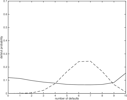
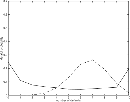
Figure 1: Loss distribution in $[0,T]$, $T=1$, of system (3), (11), (24), (25), (26), (2) when $N=10$, $\mu_{a}=0.1$, $\mu_{l}=0.1$, $\sigma_{a}=\sigma_{1,t}$, $\sigma_{l}=0.6$, $\rho_{a}=0$, $\rho_{l}=0$, $\varphi_{t}=0.1$, $\phi_{t}=0.06$, $\alpha_{t}=10,$ $\gamma_{t}=10$, $t\in[0,T]$, $T=1$ (solid line) and loss distribution in $[0,T]$, $T=1$, of system (3), (5), (6), (7) when $N=10$, $\mu_{a}=0.1$, $\mu_{l}=0.1$, $\sigma_{a}=\sigma_{1,t}$, $\sigma_{l}=0.6$, $\rho_{a}=0$, $\rho_{l}=0$, $t\in[0,T]$, $T=1$ (dashed line).

Figure 2: Loss distribution in $[0,T]$, $T=1$, of system (3), (11), (24), (25), (26), (2) when $N=10$, $\mu_{a}=0.1$, $\mu_{l}=0.1$, $\sigma_{a}=\sigma_{2,t}$, $\sigma_{l}=0.6$, $\rho_{a}=0$, $\rho_{l}=0$, $\varphi_{t}=0.1$, $\phi_{t}=0.06$, $\alpha_{t}=20,$ $\gamma_{t}=20$, $t\in[0,T]$, $T=1$ (solid line) and loss distribution in $[0,T]$, $T=1$, of system (3), (5), (6), (7) when $N=10$, $\mu_{a}=0.1$, $\mu_{l}=0.1$, $\sigma_{a}=\sigma_{2,t}$, $\sigma_{l}=0.6$, $\rho_{a}=0$, $\rho_{l}=0$, $t\in[0,T]$, $T=1$ (dashed line).

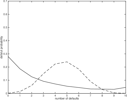
Figure 3: Loss distribution in $[0,T]$, $T=1$, of system (3), (11), (24), (25), (26), (2) when $N=10$, $\mu_{a}=0.1$, $\mu_{l}=0.1$, $\sigma_{a}=\sigma_{3,t}$, $\sigma_{l}=0.6$, $\rho_{a}=0$, $\rho_{l}=0$, $\varphi_{t}=0.1$, $\phi_{t}=0.06$, $\alpha_{t}=10,$ $\gamma_{t}=10$, $t\in[0,T]$, $T=1$ (solid line) and loss distribution in $[0,T]$, $T=1$, of system (3), (5), (6), (7) when $N=10$, $\mu_{a}=0.1$, $\mu_{l}=0.1$, $\sigma_{a}=\sigma_{3,t}$, $\sigma_{l}=0.6$, $\rho_{a}=0$, $\rho_{l}=0$, $t\in[0,T]$, $T=1$ (dashed line).

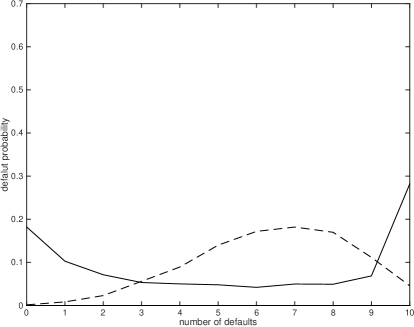
Figure 4: Loss distribution in $[0,T]$, $T=1$, of system (3), (11), (24), (25), (26), (2) when $N=10$, $\mu_{a}=0.1$, $\mu_{l}=0.1$, $\sigma_{a}=\sigma_{1,t}$, $\sigma_{l}=0.6$, $\rho_{a}=0.5$, $\rho_{l}=0$, $\varphi_{t}=0.1$, $\phi_{t}=0.06$, $\alpha_{t}=10,$ $\gamma_{t}=10$, $t\in[0,T]$, $T=1$ (solid line) and loss distribution in $[0,T]$, $T=1$, of system (3), (5), (6), (7) when $N=10$, $\mu_{a}=0.1$, $\mu_{l}=0.1$, $\sigma_{a}=\sigma_{1,t}$, $\sigma_{l}=0.6$, $\rho_{a}=0.5$, $\rho_{l}=0$, $t\in[0,T]$, $T=1$ (dashed line).

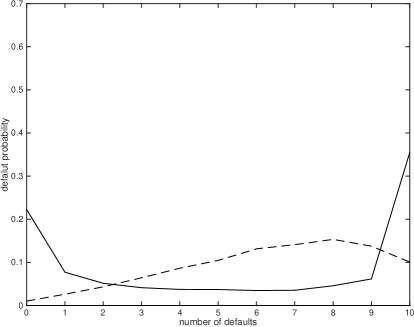
Figure 5: Loss distribution in $[0,T]$, $T=1$, of system (3), (11), (24), (25), (26), (2) when $N=10$, $\mu_{a}=0.1$, $\mu_{l}=0.1$, $\sigma_{a}=\sigma_{1,t}$, $\sigma_{l}=0.6$, $\rho_{a}=\sqrt{0.5}$, $\rho_{l}=0$, $\varphi_{t}=0.1$, $\phi_{t}=0.06$, $\alpha_{t}=10,$ $\gamma_{t}=10$, $t\in[0,T]$, $T=1$ (solid line) and loss distribution in $[0,T]$, $T=1$, of system (3), (5), (6), (7) when $N=10$, $\mu_{a}=0.1$, $\mu_{l}=0.1$, $\sigma_{a}=\sigma_{1,t}$, $\sigma_{l}=0.6$, $\rho_{a}=\sqrt{0.5}$, $\rho_{l}=0$, $t\in[0,T]$, $T=1$ (dashed line).

In Figures 2-5 the dashed line shows the loss distribution of the banks defaulted in the time interval $[0,T]$, $T=1$, of model (3), (5), (6), (7), (2), while the solid line shows the loss distribution of the banks defaulted in the time interval $[0,T]$, $T=1$, of model (3), (11), (24), (25), (26), (2) when in Figures 2-5 we have: $N=10$, $\varphi_{t}=0.1$, $\phi_{t}=0.06$, $\sigma_{l}=\sigma_{l,t}=0.6$, $\rho_{l}=\rho_{l,t}=0$, $t\in[0,T]$, $T=1$, $\mu_{a}=0.1$, $\mu_{l}=0.1$; moreover in Figure 2 we have: $\sigma_{a}=\sigma_{1,t}$, $\rho_{a}=\rho_{a,t}=0$, $\alpha_{t}=10,$ $\gamma_{t}=10$, $t\in[0,T]$, $T=1$, in Figure 2 we have: $\sigma_{a}=\sigma_{2,t}$, $\rho_{a}=\rho_{a,t}=0$, $\alpha_{t}=20,$ $\gamma_{t}=20$, $t\in[0,T]$, $T=1$, in Figure 3 we have: $\sigma_{a}=\sigma_{3,t}$, $\rho_{a}=\rho_{a,t}=0$, $\alpha_{t}=10,$ $\gamma_{t}=10$, $t\in[0,T]$, $T=1$, in Figure 4 we have: $\sigma_{a}=\sigma_{1,t}$, $\rho_{a}=\rho_{a,t}=0.5$, $\alpha_{t}=10,$ $\gamma_{t}=10$, $t\in[0,T]$, $T=1$, and finally in Figure 5 we have: $\sigma_{a}=\sigma_{1,t}$, $\rho_{a}=\rho_{a,t}=\sqrt{0.5}$, $\alpha_{t}=10,$ $\gamma_{t}=10$, $t\in[0,T]$, $T=1$.

Note that the results shown in Figures 2-5 are obtained when the functions $\varphi_{t}=0.1$, $\phi_{t}=0.06$, $t\in[0,T]$, $T=1$, are constants. With this choice there is no intervention of the monetary authority in the banking system dynamics for $t\in(0,T]$ (in fact $d\ln(\varphi_{t})=d\ln(\phi_{t})=0$, $t\in(0,T]$, in (24), (25)) and only the cooperation mechanism among banks is active when $t\in[0,T]$. Note that in Figures 2-5 also the functions $\alpha_{t}$, $\gamma_{t}$, $t\in[0,T]$, $T=1$, are chosen as constants.

For model (3), (5), (6), (7), (2) the loss distribution of the banks defaulted in $[0,T]$, $T=1$ (shown with a dashed line in Figures 2-5) is a unimodal distribution with a unique maximum corresponding to a maximizer (or to several adjacent maximizers) located in the interior of the interval $[0,N]$, $N=10$. Instead when we consider model (3), (11), (24), (25), (26), (2) the loss distribution of the banks defaulted in the time interval $[0,T]$, $T=1$ (shown with a solid line in Figures 2-5) has a bump near zero defaults and a bump near $N$ defaults and is small in between, that is is a bimodal distribution with two maxima corresponding to two maximizers (or to two disjoint sets of adjacent maximizers) located at the endpoints of the interval $[0,N]$, $N=10$. This is due to the action of the cooperation mechanism among banks in model (3), (11), (24), (25), (26), (2). Moreover the comparison between Figure 2 and Figures 4, 5 shows that the presence of a non zero correlation (i.e. $\rho_{a}\neq 0$, $\rho_{l}=0$) between the stochastic differentials on the right hand side of the assets equations of the banks (Figures 4, 5) increases substantially the probability of “extreme” systemic risk with respect to the probability of the same event in the zero correlation case (i.e. $\rho_{a}=\rho_{l}=0$) (Figure 2). Similar phenomena appear when volatility and correlation coefficient jumps are present in the liabilities equations.

Figures 2-5 show that in a homogeneous bank population the cooperation among banks introduced in model (3), (11), (24), (25), (26), (2) reduces the default probability of the individual bank when compared to the default probability of the individual bank in model (3), (5), (6), (7), (2) at the expenses of the default probability of the entire (or of almost the entire) banking system that is greater in model (3), (11), (24), (25), (26), (2) than in model (3), (5), (6), (7), (2). Moreover the comparison of Figure 2 and Figures 4, 5 shows that this effect is enhanced by the presence of “collective” behaviours in the bank population (i.e. is enhanced when $\rho_{a}^{2}$, $\rho_{l}^{2}$ are greater than zero). This is in agreement with the findings of [1], [3], [7], [10], where it is shown that for the stability of a banking system an excessive homogeneity of the bank population is undesirable.

4 The mean field approximation and the pseudo mean field approximation

For a survey of the mean field approximation in the context of statistical mechanics, see, for example, [5], and the references therein. We limit our attention to the use of some ideas taken from the mean field approximation of statistical mechanics in the study of the banking system models considered in the previous Sections.

Let us begin considering the mean field approximation of the banking system model (3), (11), (24), (25), (26), (2). When the stochastic differentials of the equations (24), (25) $dW_{t}^{i}$, $dZ_{t}^{i}$, $t\geq 0$, $i=1,2,\ldots,N$, are independent, that is when in (2) we have: $\rho_{a}^{2}=\rho_{a,t}^{2}=0$, $\rho_{l}^{2}=\rho_{l,t}^{2}=0$, $t\geq 0$, so that in (9), (10) we have: $dW_{t}^{i}=d\widetilde{W}_{t}^{i}$, $dZ_{t}^{i}=d\widetilde{Z}_{t}^{i}$, $t\geq 0$, $i=1,2,\ldots,N$, the mean field approximation of the banking system model (3), (11), (24), (25), (26), (2) can be deduced proceeding as done in [4], [3]. In fact when $\rho_{a}^{2}=\rho_{a,t}^{2}=0$, $\rho_{l}^{2}=\rho_{l,t}^{2}=0$, $t\geq 0$, and $N$ goes to infinity, it is easy to see that the mean field limit of (3), (11), (24), (25), (26), (2) is given by:

$${\cal Y}_{t}={\cal A}_{t}-{\cal L}_{t},\quad t\geq 0,$$ (32)

where

$${\cal A}_{t}=e^{{\cal G}_{t}},\quad{\cal L}_{t}=e^{{\cal H}_{t}},\quad t\geq 0,$$ (33)

and ${\cal G}_{t}$, ${\cal H}_{t}$, $t\geq 0$, satisfy the stochastic differential equations:

$$d\left({\cal G}_{t}-\ln(\varphi_{t})\right)=\alpha_{t}\left(\ln(\varphi_{t})-{\cal G}_{t}\right)dt+\sigma_{a}dP_{t},\quad t>0,$$ (34)

$$d\left({\cal H}_{t}-\ln(\phi_{t})\right)=\gamma_{t}\left(\ln(\phi_{t})-{\cal H}_{t}\right)dt+\sigma_{l}dQ_{t},\quad t>0,$$ (35)

with the initial conditions:

$${\cal G}_{0}=\ln(\varphi_{0}),\quad{\cal H}_{0}=\ln(\phi_{0}).$$ (36)

The stochastic processes $P_{t}$, $Q_{t}$, $t\geq 0$, of (34), (35) are standard Wiener processes such that $P_{0}=0$, $Q_{0}=0$, $dP_{t},$ $dQ_{t},$ $t>0$, are their stochastic differentials and we have:

$$\mathbb{E}(dP_{t}dQ_{t})=0,\quad t>0.$$ (37)

In the mean field approximation (32), (33), (34), (35), (36), (37) the stochastic process ${\cal Y}_{t}$, $t>0$, represents the capital reserves of the “mean bank” at time $t\geq 0$. Similarly the stochastic processes ${\cal A}_{t}$, ${\cal L}_{t}$, $t>0$, represent, respectively, the assets and the liabilities of the “mean bank” at time $t\geq 0$. Due to the homogeneity of the bank population, when $N$ goes to infinity the assets, the liabilities and the capital reserves of the banks of model (3), (11), (24), (25), (26), (2) behave, respectively, like the assets, the liabilities and the capital reserves of the “mean bank”, that is behave like the stochastic processes defined in (33), (32).

Let us consider the banking system model (3), (11), (24), (25), (26), (2) when the stochastic differentials of equations (24), (25) are correlated, that is when $\rho_{a}$, $\rho_{l}$ are non zero constants. Also in this case it is not difficult to deduce the mean field approximation of the banking system model (see, for example, [1]), however, for later convenience, we prefer to introduce a heuristic approximation of model (3), (11), (24), (25), (26), (2) in the limit $N$ goes to infinity that we call pseudo mean field approximation that will be used in Sections 5 and 6 to govern the probability of systemic risk in a bounded time interval. In the pseudo mean field approximation of the banking system model (3), (11), (24), (25), (26), (2) the equations (34), (35) are substituted, respectively, with the equations:

$$d\left({\cal G}_{t}-\ln(\varphi_{t})\right)=\alpha_{t}\left(1-|\rho_{a}|\right)\left(\ln(\varphi_{t})-{\cal G}_{t}\right)dt+$$

$$\hskip 91.04872ptg_{t}\,|\rho_{a}|\left(\ln(\phi_{t})-{\cal H}_{t}\right)dt+\sigma_{a}dP_{t},\quad t>0,$$ (38)

$$d\left({\cal H}_{t}-\ln(\phi_{t})\right)=\gamma_{t}\left(1-|\rho_{l}|\right)\left(\ln(\phi_{t})-{\cal H}_{t}\right)dt+$$

$$\hskip 91.04872pth_{t}\,|\rho_{l}|\left(\ln(\varphi_{t})-{\cal G}_{t}\right)dt+\sigma_{l}dQ_{t},\quad t>0.$$ (39)

The equations (38), (39) are equipped with the initial conditions (36) and the assumption (37). The functions $g_{t}\geq 0$, $h_{t}\geq 0$, $t\geq 0$, are non negative functions that will be chosen later. The pseudo mean field approximation is completed adding the equations (32), (33) to the equations (38), (39), (36), (37). In the pseudo mean field approximation (32), (33), (38), (39), (36), (37) the stochastic processes ${\cal Y}_{t}$, ${\cal A}_{t}$, ${\cal L}_{t}$, $t\geq 0,$ have the same meaning than in the mean field approximation, that is they represent, respectively, the capital reserves, the assets and the liabilities of the “pseudo mean bank” as functions of time. The equations (32), (33), (38), (39), (36), (37) define the dynamics of the “pseudo mean bank”.

When $N$ goes to infinity and the functions $g_{t}$, $h_{t}$, $t\geq 0$, are chosen appropriately, the “pseudo mean bank” behaviour “approximates” the behaviour of the “mean bank” and as a consequence “approximates” the behaviour of the banks of model (3), (11), (24), (25), (26), (2). The choice of (32), (33), (38), (39), (36), (37) and in particular the choice of (38), (39) as pseudo mean field approximation is motivated by the following facts. First of all when the stochastic differentials $dW_{t}^{i}$, $dZ_{t}^{i}$, $t>0$, $i=1,2,\ldots,N$, of equations (24), (25) are independent, that is when in (2) we have $\rho_{a}^{2}=0$, $\rho_{l}^{2}=0$, $t>0$, the pseudo mean field approximation (32), (33), (38), (39), (36), (37) coincides with the mean field approximation (32), (33), (34), (35), (36), (37). Moreover when in the equations (24), (25) the stochastic differentials $dW_{t}^{i}$, $t>0$, $i=1,2,\ldots,N$, and $dZ_{t}^{i}$, $t>0$, $i=1,2,\ldots,N$, are totally correlated, that is when we have $|\rho_{a}|=1$, $|\rho_{l}|=1$, and we choose $g_{t}=0$, $h_{t}=0$, $t>0$, the pseudo mean field approximation (32), (33), (38), (39), (36), (37) “coincides” with the banking system model (3), (11), (24), (25), (26), (2), with $|\rho_{a}|=1$, $|\rho_{l}|=1$, $t>0$. That is the pseudo mean field approximation is “exact”. In fact when $|\rho_{a}|=1$, $|\rho_{l}|=1$, $t>0$, the initial conditions $G_{0}^{i}=\ln(\varphi_{0}),$ $H_{0}^{i}=\ln(\phi_{0}),$ $i=1,2,\ldots,N$, imply that the cooperation mechanism among banks present in (24) and in (25) has no influence on the banking system dynamics. In fact the previous choices imply that in (24) $\alpha_{t}$, $t\geq 0$, multiplies the null term, that is imply that $\displaystyle\sum_{j=1}^{N}\left(G_{t}^{j}-G_{t}^{i}\right)dt=0$, $t>0$. Similarly the previous choices imply that in (25) $\gamma_{t}$, $t\geq 0$, multiplies the null term, that is imply that $\displaystyle\sum_{j=1}^{N}\left(H_{t}^{j}-H_{t}^{i}\right)dt=0$, $t>0$. In fact when $|\rho_{a}|=1$, $|\rho_{l}|=1$, $t>0$, and $G_{0}^{i}=\ln(\varphi_{0}),$ $H_{0}^{i}=\ln(\phi_{0}),$ $i=1,2,\ldots,N$, all the banks of the model satisfy the same equation and can be considered as a “unique” bank repeated $N$ times. Note that the condition $|\rho_{a}|=1$, $|\rho_{l}|=1$, $t>0$, implies that the Wiener processes present in the equations relative to the different banks of the model coincide, that is $dW_{t}^{i}$, $dZ_{t}^{i}$, $t>0$, in (24), (25) do not depend on $i$, $i=1,2,\ldots,N$. In this case all the banks of the banking system model are replicated exactly by the pseudo mean field approximation (32), (33), (38), (39), (36), (37) when $|\rho_{a}|=1$, $|\rho_{l}|=1$, $t>0$, and we choose $g_{t}=0$, $h_{t}=0$, $t>0$. When in the equations (24), (25) the stochastic differentials $dW_{t}^{i}$, $dZ_{t}^{i}$, $t>0$, $i=1,2,\ldots,N$, are partially correlated, that is when in (2) we have $0<|\rho_{a}|<1$, $0<|\rho_{l}|<1$, $t>0$, choosing appropriately the functions $g_{t}$, $h_{t}$, $t>0$, the pseudo mean field approximation (32), (33), (38), (39), (36), (37) “interpolates” between the extreme cases $\rho_{a}=0$, $\rho_{l}=0$, $t>0$, and $|\rho_{a}|=1$, $|\rho_{l}|=1$, $t>0$. Finally in Section 6 in the systemic risk governance the form chosen for the equations (38), (39) will make possible the use of the polynomial identity principle to determine the functions $\alpha_{t}$, $\gamma_{t}$, $t\geq 0$, that regulate the cooperation mechanism among banks.

In Section 6 we explain the choice of the functions $\varphi_{t}$, $\phi_{t}$, $\alpha_{t}$, $\gamma_{t}$, $g_{t}$, $h_{t}$, $t\geq 0$, that is used to govern the systemic risk probability in a bounded time interval of model (3), (11), (24), (25), (26), (2).

Note that when $\alpha_{t}=0$, $\gamma_{t}=0$, $t\geq 0$, and the functions $\varphi_{t}$, $\phi_{t}$, $t\geq 0$, are positive constants, there is no cooperation among banks and no intervention of the monetary authority in the banking system dynamics. In this case in the pseudo mean field approximation we choose $g_{t}=0$, $h_{t}=0$, $t\geq 0$.

5 An optimal control problem for the pseudo mean field approximation

Let us consider an optimal control problem for the pseudo mean field approximation (32), (33), (38), (39), (36), (37) of the banking system model (3), (11), (24), (25), (26), (2) when $0\leq|\rho_{a}|<1$, $0\leq|\rho_{l}|<1$, $t>0$. Let $n$ be a positive integer, $\mathbb{R}$ be the set of real numbers, $\mathbb{R}^{n}$ be the $n$-dimensional real Euclidean space and $\mathbb{R}^{+}$ be the set of the positive real numbers.

Given the positive functions $\varphi_{t}$, $\phi_{t}$, $t\geq 0$, we define:

$${\cal Z}_{t}={\cal G}_{t}-\ln(\varphi_{t}),\quad t\geq 0,$$ (40)

and

$${\cal S}_{t}={\cal H}_{t}-\ln(\phi_{t}),\quad t\geq 0,$$ (41)

equations (38), (39), (36) can be rewritten as follows:

$$d{\cal Z}_{t}=\beta_{a}(t,{\cal Z}_{t},{\cal S}_{t})dt+\sigma_{a}dP_{t},\,\,t>0,\$$ (42)

$$d{\cal S}_{t}=\beta_{l}(t,{\cal Z}_{t},{\cal S}_{t})dt+\sigma_{l}dQ_{t},\,\,t>0,\$$ (43)

$${\cal Z}_{0}=0,\quad{\cal S}_{0}=0,$$ (44)

where $\beta_{a}:\mathbb{R}^{+}\times\mathbb{R}^{2}\rightarrow\mathbb{R}$ and $\beta_{l}:\mathbb{R}^{+}\times\mathbb{R}^{2}\rightarrow\mathbb{R}$ are given by:

$$\hskip-28.45274pt\beta_{a}=\beta_{a,t}=\beta_{a}(t,{\cal Z},{\cal S})=-\alpha_{t}\left(1-|\rho_{a}|\right){\cal Z}-|\rho_{a}|\,g_{t}\,{\cal S},\quad({\cal Z},{\cal S})\in\mathbb{R}^{2},\,\,t>0,$$ (45)

$$\hskip-28.45274pt\beta_{l}=\beta_{l,t}=\beta_{l}(t,{\cal Z},{\cal S})=-\gamma_{t}\left(1-|\rho_{l}|\right){\cal S}-|\rho_{l}|\,h_{t}\,{\cal Z},\quad({\cal Z},{\cal S})\in\mathbb{R}^{2},\,\,t>0,$$ (46)

and in (44) the symbol $0$ denotes the random variable concentrated in zero with probability one.

To choose the functions $\alpha_{t}$, $\gamma_{t}$, $g_{t}$, $h_{t}$, $t>0$, of (45), (46) as done in the systemic risk governance of Section 6 we begin solving the stochastic optimal control problem that follows.

Let $T_{1}>0$ be a real number, $\boldsymbol{\lambda}=(\lambda_{1},\lambda_{2},\lambda_{3},\lambda_{4})\in\mathbb{R}^{4}$, $\lambda_{i}>0$, $i=1,2,3,4$, and $\mathcal{B}$ be the set of the real square integrable stochastic processes defined in $[0,T_{1}]$, that is a real stochastic process $\zeta=\zeta_{t},$ $t\in[0,T_{1}]$, belongs to $\mathcal{B}$ if and only if $\displaystyle\mathbb{E}\left(\int_{0}^{T_{1}}\zeta_{t}^{2}\,dt\right)<+\infty$. We consider the following stochastic optimal control problem:

$$\min_{\beta_{1},\beta_{2}\in\mathcal{B}}U_{\boldsymbol{\lambda}}(\beta_{1},\beta_{2}),$$ (47)

where

$$\hskip-19.91684ptU_{\boldsymbol{\lambda}}(\beta_{1},\beta_{2})=$$

$$\hskip-19.91684pt\mathbb{E}\left(\int_{0}^{T_{1}}\left[|\rho_{a}\rho_{l}|({\cal Z}_{t}-{\cal S}_{t})^{2}+\lambda_{1}\beta_{1,t}^{2}+\lambda_{2}\beta_{2,t}^{2}+\lambda_{3}(1-|\rho_{a}|){\cal Z}_{t}^{2}+\lambda_{4}(1-|\rho_{l}|){\cal S}_{t}^{2}\right]dt\right),$$

$$\hskip 56.9055pt\beta_{1},\,\beta_{2}\in\mathcal{B},\,0\leq|\rho_{a}|<1,\,0\leq|\rho_{l}|<1,\,\$$ (48)

subject to

$$d{\cal Z}_{t}=\beta_{1}\,dt+\sigma_{a}dP_{t},\quad t\in[0,T_{1}],$$ (49)

$$d{\cal S}_{t}=\beta_{2}\,dt+\sigma_{l}dQ_{t},\quad t\in[0,T_{1}],$$ (50)

$${\cal Z}_{0}=0,\quad{\cal S}_{0}=0.$$ (51)

In the control problem (47), (48), (49), (50), (51) the function $U_{\boldsymbol{\lambda}}(\beta_{1},\beta_{2})$ is the utility function, $\beta_{1}=\beta_{1,t}=\beta_{1}(t,{\cal Z}_{t},{\cal S}_{t}),$ $\beta_{2}=\beta_{2,t}=\beta_{2}(t,{\cal Z}_{t},{\cal S}_{t}),$ $t\in[0,T_{1}],$ are the control variables and ${\cal Z}_{t}$, ${\cal S}_{t}$, $t\in[0,T_{1}],$ are the state variables. The random variables on the right hand side of equation (51) must be interpreted as already done for those of equation (44).

When $0<|\rho_{a}|<1$, $0<|\rho_{l}|<1$, minimizing the utility function $U_{\boldsymbol{\lambda}}(\beta_{1},\beta_{2})$, $\beta_{1}=\beta_{1,t},$ $\beta_{2}=\beta_{2,t},$ $t\in[0,T_{1}],$ defined in (48) means making small in the time interval $[0,T_{1}]$ the following quantities: ${\it i)}$ the difference between the capital reserves of the “pseudo mean bank” and the capital reserves of the “ideal bank” ${\cal Z}_{t}-{\cal S}_{t}=({\cal G}_{t}-\ln(\varphi_{t}))-({\cal H}_{t}-\ln(\phi_{t}))$, $t\in[0,T_{1}]$, ${\it ii)}$ the “size” of the control variable $\beta_{1,t}$, $t\in[0,T_{1}]$, ${\it iii)}$ the “size” of the control variable $\beta_{2,t}$, $t\in[0,T_{1}]$, ${\it iv)}$ the “size” of ${\cal Z}_{t}$, $t\in[0,T_{1}]$ (and therefore the difference between ${\cal G}_{t}$, $t\in[0,T_{1}]$, and the function $\ln(\varphi_{t})$, $t\in[0,T_{1}]$), ${\it v)}$ the “size” of ${\cal S}_{t}$, $t\in[0,T_{1}]$ (and therefore the difference between ${\cal H}_{t}$, $t\in[0,T_{1}]$, and the function $\ln(\phi_{t})$, $t\in[0,T_{1}]$). These five goals correspond, respectively, to making small the addenda: i) $\displaystyle\mathbb{E}\left(\int_{0}^{T_{1}}|\rho_{a}\rho_{l}|({\cal Z}_{t}-{\cal S}_{t})^{2}dt\right)$, ii) $\displaystyle\mathbb{E}\left(\int_{0}^{T_{1}}\lambda_{1}\beta_{1,t}^{2}\,dt\right)$, iii) $\displaystyle\mathbb{E}\left(\int_{0}^{T_{1}}\lambda_{2}\beta_{2,t}^{2}\,dt\right)$, iv) $\displaystyle\mathbb{E}\left(\int_{0}^{T_{1}}\lambda_{3}(1-|\rho_{a}|){\cal Z}_{t}^{2}\,dt\right)$, v) $\displaystyle\mathbb{E}\left(\int_{0}^{T_{1}}\lambda_{4}(1-|\rho_{l}|)\right.$ $\left.{\cal S}_{t}^{2}\,dt\right)$ of the utility function $U_{\boldsymbol{\lambda}}$ defined in (48).

Note that when $\rho_{a}=0$ and/or $\rho_{l}=0$ the term $\displaystyle\mathbb{E}\left(\int_{0}^{T_{1}}|\rho_{a}\rho_{l}|({\cal Z}_{t}-{\cal S}_{t})^{2}dt\right)$ of $U_{\boldsymbol{\lambda}}$ is zero and that in this case minimizing the utility function $U_{\boldsymbol{\lambda}}$ corresponds to pursuing only four of the five goals listed above, that is corresponds to pursuing the goals of making small in the time interval $[0,T_{1}]$ the quantities ${\it ii)}$, ${\it iii)}$, ${\it iv)}$, ${\it v)}$.

The control problem (47), (48), (49), (50), (51) is a linear-quadratic optimal control problem (see [9]). Following Kalman [9] we assume that its value function is a quadratic form in the real variables ${\cal Z}$, ${\cal S}$ with time dependent coefficients. We have:

Proposition 1. Under the previous assumptions when $0\leq|\rho_{a}|<1$ and $0\leq|\rho_{l}|<1$ the optimal control $\beta_{1}=\beta_{1,t}$, $\beta_{2}=\beta_{2,t}$, $t\in[0,T_{1}]$, solution of problem (47), (48), (49), (50), (51) is given by:

$$\beta_{1}=\beta_{1,t}=\beta_{1}(t,{\cal Z}_{t},{\cal S}_{t})=-\frac{1}{2\lambda_{1}}\left(2a(t){\cal Z}_{t}+c(t){\cal S}_{t}\right),\quad t\in[0,T_{1}],$$ (52)

$$\beta_{2}=\beta_{1,t}=\beta_{2}(t,{\cal Z}_{t},{\cal S}_{t})=-\frac{1}{2\lambda_{2}}\left(2b(t){\cal S}_{t}+c(t){\cal Z}_{t}\right),\quad t\in[0,T_{1}],$$ (53)

where ${\cal Z}_{t}$, ${\cal S}_{t}$, $t\in[0,T_{1}]$, are solution of the initial value problem (49), (50), (51). The functions $a(t)$, $b(t)$, $c(t)$, $d(t)$, $t\in[0,T_{1}],$ are defined by the following final value problem:

$$\frac{\partial a}{\partial t}=\frac{a^{2}}{\lambda_{1}}+\frac{c^{2}}{4\lambda_{2}}-|\rho_{a}\rho_{l}|-\lambda_{3}(1-|\rho_{a}|),\quad\quad t\in[0,T_{1}],\hskip 28.45274pta(T_{1})=0,$$ (54)

$$\frac{\partial b}{\partial t}=\frac{b^{2}}{\lambda_{2}}+\frac{c^{2}}{4\lambda_{1}}-|\rho_{a}\rho_{l}|-\lambda_{4}(1-|\rho_{l}|),\quad\quad t\in[0,T_{1}],\hskip 31.2982ptb(T_{1})=0,$$ (55)

$$\frac{\partial c}{\partial t}=\frac{ac}{\lambda_{1}}+\frac{bc}{\lambda_{2}}+2|\rho_{a}\rho_{l}|,\hskip 93.89418ptt\in[0,T_{1}],\hskip 31.2982ptc(T_{1})=0,$$ (56)

$$\frac{\partial d}{\partial t}=-a\sigma_{a}^{2}-b\sigma_{l}^{2},\hskip 122.34692ptt\in[0,T_{1}],\hskip 31.2982ptd(T_{1})=0.$$ (57)

Note that the optimal control (52), (53) does not depend from the function $d(t)$, $t\in[0,T_{1}]$ that appears in (57); it depends only from the functions $a(t)$, $b(t)$, $c(t)$, $t\in[0,T_{1}],$ and that the final value problem (54), (55), (56) satisfied by $a(t)$, $b(t)$, $c(t)$, $t\in[0,T_{1}],$ can be solved independently from the final value problem (57) satisfied by $d(t)$, $t\in[0,T_{1}]$. However the function $d(t)$, $t\in[0,T_{1}]$ is necessary to define the value function $V$ (see (63)) of the control problem (47), (48), (49), (50), (51) and the formulae (52), (53) for the optimal control are deduced from the expression of the value function.

Proof. Let us use the dynamic programming principle (see [9]) to solve the control problem (47), (48), (49), (50), (51). That is let

$$\hskip-28.45274ptV(t,{\cal Z},{\cal S})=\min_{\beta_{1},\beta_{2}\in\mathcal{B}}\mathbb{E}\left(\int_{t}^{T_{1}}\left[|\rho_{a}\rho_{l}|({\cal Z}_{\tau}-{\cal S}_{\tau})^{2}+\lambda_{1}\beta_{1,\tau}^{2}+\lambda_{2}\beta_{2,\tau}^{2}+\lambda_{3}(1-|\rho_{a}|){\cal Z}_{\tau}^{2}+\right.\right.$$

$$\hskip 56.9055pt\left.\left.\lambda_{4}(1-|\rho_{l}|){\cal S}_{\tau}^{2}\right]d\tau\Big{|}{\cal Z}_{t}={\cal Z},{\cal S}_{t}={\cal S}\right),\,\,({\cal Z},{\cal S})\in\mathbb{R}^{2},\,t\in[0,T_{1}],$$ (58)

be the value function of the control problem (47), (48), (49), (50), (51). The function $V(t,{\cal Z},{\cal S})$, $({\cal Z},{\cal S})\in\mathbb{R}^{2},$ $t\in[0,T_{1}]$, satisfies the following Hamilton, Jacobi, Bellman equation (see [9]):

$$\frac{\partial}{\partial t}V(t,{\cal Z},{\cal S})+\frac{1}{2}\sigma_{a}^{2}\frac{\partial^{2}}{\partial{\cal Z}^{2}}V(t,{\cal Z},{\cal S})+\frac{1}{2}\sigma_{l}^{2}\frac{\partial^{2}}{\partial{\cal S}^{2}}V(t,{\cal Z},{\cal S})+|\rho_{a}\rho_{l}|\left({\cal Z}-{\cal S}\right)^{2}+$$

$$\lambda_{3}(1-|\rho_{a}|){\cal Z}^{2}+\lambda_{4}(1-|\rho_{l}|){\cal S}^{2}+\mathcal{H}\left(\frac{\partial}{\partial{\cal Z}}V(t,{\cal Z},{\cal S}),\frac{\partial}{\partial{\cal S}}V(t,{\cal Z},{\cal S})\right)=0,$$

$$\hskip 199.16928pt({\cal Z},{\cal S})\in\mathbb{R}^{2},\,t\in[0,T_{1}],$$ (59)

with final condition:

$$V(T_{1},{\cal Z},{\cal S})=0,\quad({\cal Z},{\cal S})\in\mathbb{R}^{2},$$ (60)

where

$$\mathcal{H}(p_{1},p_{2})=\min_{(\delta_{1},\delta_{2})\in\mathbb{R}^{2}}\left(\delta_{1}p_{1}+\lambda_{1}\delta_{1}^{2}+\delta_{2}p_{2}+\lambda_{2}\delta_{2}^{2}\right)=-\frac{p_{1}^{2}}{4\lambda_{1}}-\frac{p_{2}^{2}}{4\lambda_{2}},\quad(p_{1},p_{2})\in\mathbb{R}^{2},$$ (61)

is the Hamiltonian function of the optimal control problem (47), (48), (49), (50), (51).
Using (61) equation (59) becomes:

$$\frac{\partial}{\partial t}V(t,{\cal Z},{\cal S})+\frac{1}{2}\sigma_{a}^{2}\frac{\partial^{2}}{\partial{\cal Z}^{2}}V(t,{\cal Z},{\cal S})+\frac{1}{2}\sigma_{l}^{2}\frac{\partial^{2}}{\partial{\cal S}^{2}}V(t,{\cal Z},{\cal S})+|\rho_{a}\rho_{l}|\left({\cal Z}-{\cal S}\right)^{2}+$$

$$\quad\quad\lambda_{3}(1-|\rho_{a}|){\cal Z}^{2}+\lambda_{4}(1-|\rho_{l}|){\cal S}^{2}-\frac{1}{4\lambda_{1}}\left(\frac{\partial}{\partial{\cal Z}}V(t,{\cal Z},{\cal S})\right)^{2}-$$

$$\quad\quad\frac{1}{4\lambda_{2}}\left(\frac{\partial}{\partial{\cal S}}V(t,{\cal Z},{\cal S})\right)^{2}=0,\quad({\cal Z},{\cal S})\in\mathbb{R}^{2},\,t\in[0,T_{1}],$$ (62)

with the final condition (60).
Following Kalman [9] we assume that the value function solution of problem (62), (60) is of the form:

$$V(t,{\cal Z},{\cal S})=a(t){\cal Z}^{2}+b(t){\cal S}^{2}+c(t){\cal Z}{\cal S}+d(t),\quad\quad({\cal Z},{\cal S})\in\mathbb{R}^{2},\,\,t\in[0,T_{1}],$$ (63)

where $a(t)$, $b(t)$, $c(t)$, $d(t)$, $t\in[0,T_{1}],$ are functions to be determined.
Substituting (63) in (62), (60) and using the polynomial identity principle it is easy to see that the final value problem for the Hamilton, Jacobi, Bellman equation (62), (60) reduces to the final value problem (54), (55), (56), (57).

Problem (54), (55), (56), (57) is a final value problem for a system of Riccati ordinary differential equations. In general systems of this kind have only local solutions. This means that, in general, a solution of (54), (55), (56), (57) in the time interval $[0,T_{1}]$ may not exist. When this is the case the assumption (63) about the form of the value function is not good enough to solve problem (47), (48), (49), (50), (51) and we do not go any further in the study of the control problem (47), (48), (49), (50), (51). From now on we assume that the final value problem (54), (55), (56), (57) has a solution defined in $[0,T_{1}]$.

From the knowledge of the value function $V$ defined in (63) solution of (62), (60) the optimal control $\beta_{1}=\beta_{1,t}$, $\beta_{2}=\beta_{2,t}$, $t\in[0,T_{1}],$ solution of (47), (48), (49), (50), (51) is determined using the formulae:

$$\hskip-14.22636pt\beta_{1}=\beta_{1,t}=\beta_{1}(t,{\cal Z}_{t},{\cal S}_{t})=-\frac{1}{2\lambda_{1}}\frac{\partial}{\partial{\cal Z}}V(t,{\cal Z},{\cal S})\Big{|}_{{\cal Z}={\cal Z}_{t},{\cal S}={\cal S}_{t}}=-\frac{1}{2\lambda_{1}}\left(2a(t){\cal Z}_{t}+c(t){\cal S}_{t}\right),$$

$$\hskip 227.62204ptt\in[0,T_{1}],$$ (64)

$$\hskip-14.22636pt\beta_{2}=\beta_{2,t}=\beta_{2}(t,{\cal Z}_{t},{\cal S}_{t})=-\frac{1}{2\lambda_{2}}\frac{\partial}{\partial{\cal S}}V(t,{\cal Z},{\cal S})\Big{|}_{{\cal Z}={\cal Z}_{t},{\cal S}={\cal S}_{t}}=-\frac{1}{2\lambda_{2}}\left(2b(t){\cal S}_{t}+c(t){\cal Z}_{t}\right),$$

$$\hskip 227.62204ptt\in[0,T_{1}],$$ (65)

where ${\cal Z}_{t}$, ${\cal S}_{t}$, $t\in[0,T_{1}]$, are the solution of (49), (50), (51) when $\beta_{1}$=$\beta_{1,t}$, $\beta_{2}$=$\beta_{2,t}$, $t\in[0,T_{1}],$ are given by (64), (65).

Problem (47), (48), (49), (50), (51) is the optimal control problem used to govern the pseudo mean field approximation (32), (33), (38), (39), (36), (37) of the banking system model (3), (11), (24), (25), (26), (2). In fact, when $0\leq|\rho_{a}|<1$, $0\leq|\rho_{l}|<1$, given the optimal control $\beta_{1}$, $\beta_{2}$ defined in (64), (65) we determine the functions $\beta_{a}$, $\beta_{l}$ of (45), (46) imposing the identities $\beta_{a}({\cal Z},{\cal S})=\beta_{1}({\cal Z},{\cal S})$, $\beta_{l}({\cal Z},{\cal S})=\beta_{2}({\cal Z},{\cal S})$, $({\cal Z},{\cal S})\in\mathbb{R}^{2},$ and using the polynomial identity principle in the variables $({\cal Z},{\cal S})\in\mathbb{R}^{2}$. We have:

$$\displaystyle\alpha_{t}=\frac{a(t)}{\lambda_{1}(1-|\rho_{a}|)},\quad\displaystyle\gamma_{t}=\frac{b(t)}{\lambda_{2}(1-|\rho_{l}|)},\quad t\in[0,T_{1}],\quad 0\leq|\rho_{a}|,|\rho_{l}|<1,$$ (66)

and

$$\displaystyle g_{t}=\frac{c(t)}{2\lambda_{1}\,|\rho_{a}|},\quad\displaystyle h_{t}=\frac{c(t)}{2\lambda_{2}\,|\rho_{l}|},\quad t\in[0,T_{1}],\quad 0<|\rho_{a}|,|\rho_{l}|<1,$$ (67)

or

$$h_{t}=0\quad\text{and/or}\quad g_{t}=0,\quad t\in[0,T_{1}],\quad\rho_{a}=0\quad\text{and/or}\quad\rho_{l}=0.$$ (68)

Let us point out that when $\rho_{a}=0$ and/or $\rho_{l}=0$ the function $c(t)=0$, $t\in[0,T_{1}]$ is a solution of (56). Moreover note that the use of the polynomial identity principle in the deduction of (66), (67), (68) is possible thanks to the form of equations (38), (39) of the pseudo mean field approximation.

Recall that the function $\alpha_{t}$, $t\in[0,T_{1}],$ defined in (66) is a function that substituted in (24) induces the trajectories of the logarithm of the assets to swarm around $\ln(\varphi_{t})$, $t\in[0,T_{1}],$ and therefore induces the trajectories of the assets to swarm around $\varphi_{t}$, $t\in[0,T_{1}].$ Similarly the function $\gamma_{t}$, $t\in[0,T_{1}],$ defined in (66) is a function that substituted in (25) induces the trajectories of the logarithms of the liabilities to swarm around $\ln(\phi_{t})$, $t\in[0,T_{1}],$ and therefore induces the trajectories of the liabilities to swarm around $\phi_{t}$, $t\in[0,T_{1}].$

Remember that in (24), (25) the constraints $\alpha_{t}\geq 0,$ $\gamma_{t}\geq 0$, $t\in[0,T_{1}]$, must be satisfied. When they are not satisfied by the choices of $\alpha_{t},$ $\gamma_{t}$, $t\in[0,T_{1}]$, made in (66) they are enforced. In the numerical experiments discussed in Section 6 when the functions $\alpha_{t}$ and/or $\gamma_{t}$, $t\in[0,T_{1}]$, determined using (66) are negative, we choose $\alpha_{t}=0$ and/or $\gamma_{t}=0$, $t\in[0,T_{1}]$.

Note that the formulae (66), (67), (68) provide a choice of the functions $\alpha_{t}$, $\gamma_{t}$, $g_{t}$, $h_{t}$ when $t\in[0,T_{1}]$; to choose the functions $\alpha_{t}$, $\gamma_{t}$, $g_{t}$, $h_{t}$ when $t>0$ the previous formulae must be adapted to take care of the repeated solution of control problems similar to the one considered here.

6 The systemic risk governance

Let $T_{2}>0$ be a real number and consider the problem of governing the probability of systemic risk in the time interval $[0,T_{2}]$ in model (3), (11), (24), (25), (26), (2) in absence or in presence of shocks acting on the banking system. Given $\tau_{1},\tau_{2}$ such that $0\leq\tau_{1}<\tau_{2}\leq T_{2}$, and the interval $[\tau_{1},\tau_{2}]\subseteq[0,T_{2}]$, let us consider the governance of systemic risk in the time interval $[\tau_{1},\tau_{2}]$. The goal of the governance is to keep the probability of systemic risk in the time interval $[\tau_{1},\tau_{2}]$, $\mathcal{P}(SR_{[\tau_{1},\tau_{2}]})$, between two given thresholds. The systemic risk governance pursues its goal trying to keep the assets, the liabilities and the capital reserves of the banks of the model “close”, respectively, to the assets, the liabilities and the capital reserves of the “ideal bank”, that is close, respectively, to the functions $\varphi_{t}>0$, $\phi_{t}>0$ and $\xi_{t}=\varphi_{t}-\phi_{t}>0$, $t\in[\tau_{1},\tau_{2}]$. Given the choice of the functions $\varphi_{t}$, $\phi_{t}$, $\xi_{t}=\varphi_{t}-\phi_{t}$, $t\in[\tau_{1},\tau_{2}]$, the governance is based on the solution of the optimal control problem (47), (48), (49), (50), (51) and on its relation with the banking system model (3), (11), (24), (25), (26), (2) when the functions $\alpha_{t}$, $\gamma_{t}$, $t\in[\tau_{1},\tau_{2}],$ are chosen adapting formula (66) deduced for the time interval $[0,T_{1}]$ to the time interval $[\tau_{1},\tau_{2}]$. In fact the choice of the functions $\alpha_{t}$, $\gamma_{t}$, $t\in[\tau_{1},\tau_{2}]$, obtained adapting formula (66) to the time interval $[\tau_{1},\tau_{2}],$ creates a “swarming” effect of the assets and of the liabilities of the banks of the model around, respectively, the functions $\varphi_{t}$, $\phi_{t}$, $t\in[\tau_{1},\tau_{2}]$, and, as a consequence, creates a “swarming” effect of the capital reserves of the banks of the model around the function $\xi_{t}$, $t\in[\tau_{1},\tau_{2}]$.

We assume that the decisions about systemic risk governance in the time interval $[\tau_{1},\tau_{2}]$ are taken at time $t=\tau_{1}$. Going into details to pursue the goal of keeping the probability of systemic risk in the time interval $[\tau_{1},\tau_{2}]$, $\mathcal{P}(SR_{[\tau_{1},\tau_{2}]})$, between two given thresholds the first thing to do at time $t=\tau_{1}$ is to choose appropriately the functions $\varphi_{t}$, $\phi_{t}$, $\xi_{t}=\varphi_{t}-\phi_{t}$, $t\in[\tau_{1},\tau_{2}]$. In fact it is easy to see that increasing $\xi_{t}>0$, $t\in[\tau_{1},\tau_{2}]$, the systemic risk probability in $[\tau_{1},\tau_{2}]$ decreases and that decreasing $\xi_{t}>0$, $t\in[\tau_{1},\tau_{2}]$, the systemic risk probability in $[\tau_{1},\tau_{2}]$ increases. Moreover, since $\xi_{t}=\varphi_{t}-\phi_{t}>0$, $t\in[\tau_{1},\tau_{2}]$, increasing $\xi_{t}$, $t\in[\tau_{1},\tau_{2}]$, can be done increasing $\varphi_{t}$ leaving unchanged $\phi_{t}$, $t\in[\tau_{1},\tau_{2}]$, or decreasing $\phi_{t}$ leaving unchanged $\varphi_{t}$, $t\in[\tau_{1},\tau_{2}]$, or changing at the same time $\varphi_{t}$ and $\phi_{t}$, $t\in[\tau_{1},\tau_{2}]$. Similarly decreasing $\xi_{t}$, $t\in[\tau_{1},\tau_{2}]$, can be done either decreasing $\varphi_{t}$ leaving unchanged $\phi_{t}$, $t\in[\tau_{1},\tau_{2}]$, or increasing $\phi_{t}$ leaving unchanged $\varphi_{t}$, $t\in[\tau_{1},\tau_{2}]$, or changing at the same time $\varphi_{t}$ and $\phi_{t}$, $t\in[\tau_{1},\tau_{2}]$.

Given the thresholds $S_{1}$, $S_{2}$, such that $0<S_{1}<S_{2}<1$, and $\varphi_{\tau_{1}}$, $\phi_{\tau_{1}}$, $\xi_{\tau_{1}}=\varphi_{\tau_{1}}-\phi_{\tau_{1}}$ we want to choose the functions $\varphi_{t}$, $\phi_{t}$, $\xi_{t}=\varphi_{t}-\phi_{t}$, $t\in[\tau_{1},\tau_{2}]$, such that the probability of systemic risk in the time interval $[\tau_{1},\tau_{2}]$ satisfies the following inequalities:

$$S_{1}\leq\mathcal{P}(SR_{[\tau_{1},\tau_{2}]})\leq S_{2}.$$ (69)

We define some simple rules that are used to choose the functions $\varphi_{t}$, $\phi_{t}$, $\xi_{t}=\varphi_{t}-\phi_{t}$, $t\in[\tau_{1},\tau_{2}]$ in order to satisfy (69). At time $t=\tau_{1}$ we start making the “simplest” possible choice of $\varphi_{t}$, $\phi_{t}$, $\xi_{t}=\varphi_{t}-\phi_{t}$, $t\in[\tau_{1},\tau_{2}]$, that is we choose: $\varphi_{t}=\varphi_{\tau_{1}}$, $\phi_{t}=\phi_{\tau_{1}}$, $\xi_{t}=\xi_{\tau_{1}}$, $t\in[\tau_{1},\tau_{2}]$. In correspondence to this choice the functions $\alpha_{t}$, $\gamma_{t}$, $t\in[\tau_{1},\tau_{2}]$, are determined adapting formula (66) to the time interval $[\tau_{1},\tau_{2}]$ and the probability of systemic risk in the time interval $[\tau_{1},\tau_{2}]$, $\mathcal{P}(SR_{[\tau_{1},\tau_{2}]})$, is evaluated using statistical simulation. Note that $\mathcal{P}(SR_{[\tau_{1},\tau_{2}]})$ depends not only from the functions $\varphi_{t}$, $\phi_{t}$, $\alpha_{t}$, $\gamma_{t}$, $t\in[\tau_{1},\tau_{2}]$, but also from the random variables $a_{\tau_{1}}^{i}$, $l_{\tau_{1}}^{i}$, $c_{\tau_{1}}^{i}=a_{\tau_{1}}^{i}-l_{\tau_{1}}^{i}$, $i=1,2,\ldots,N$. Based on the value of $\mathcal{P}(SR_{[\tau_{1},\tau_{2}]})$ the following actions are taken:

1. Strategy 1: if $\mathcal{P}(SR_{[\tau_{1},\tau_{2}]})>S_{2}$ the monetary authority changes the functions $\varphi_{t}$, $\phi_{t}$, $\xi_{t}=\varphi_{t}-\phi_{t}$, $t\in[\tau_{1},\tau_{2}]$, to “swarm” the trajectories of the capital reserves of the banking system model (3), (11), (24), (25), (26), (2) “upward”, that is the monetary authority increases $\xi_{t}>0$, $t\in[\tau_{1},\tau_{2}]$. This is done in one of the following ways:

   1. Strategy 1a: increasing $\varphi_{t}>0$ leaving unchanged $\phi_{t}>0$, $t\in[\tau_{1},\tau_{2}]$;

   2. Strategy 1b: decreasing $\phi_{t}>0$ leaving unchanged $\varphi_{t}>0$, $t\in[\tau_{1},\tau_{2}]$;

   3. Strategy 1c: changing both $\varphi_{t}>0$ and $\phi_{t}>0$, $t\in[\tau_{1},\tau_{2}]$.

2. Strategy 2: if $\mathcal{P}(SR_{[\tau_{1},\tau_{2}]})<S_{1}$ the monetary authority changes the functions $\varphi_{t}$, $\phi_{t}$, $\xi_{t}=\varphi_{t}-\phi_{t}$, $t\in[\tau_{1},\tau_{2}]$, to “swarm” the trajectories of the capital reserves of the banking system model (3), (11), (24), (25), (26), (2) “downward”, that is the monetary authority decreases $\xi_{t}>0$, $t\in[\tau_{1},\tau_{2}]$. This is done in one of the following ways:

   1. Strategy 2a: decreasing $\varphi_{t}>0$ leaving unchanged $\phi_{t}>0$, $t\in[\tau_{1},\tau_{2}]$;

   2. Strategy 2b: increasing $\phi_{t}>0$ leaving unchanged $\varphi_{t}>0$, $t\in[\tau_{1},\tau_{2}]$;

   3. Strategy 2c: changing both $\varphi_{t}>0$ and $\phi_{t}>0$, $t\in[\tau_{1},\tau_{2}]$.

3. Strategy 3: if $S_{1}\leq\mathcal{P}(SR_{[\tau_{1},\tau_{2}]})\leq S_{2}$ the monetary authority leaves the functions $\varphi_{t}$, $\phi_{t}$, $\xi_{t}=\varphi_{t}-\phi_{t}$, $t\in[\tau_{1},\tau_{2}]$, unchanged.

Note that at time $t=\tau_{1}$ the monetary authority makes its decisions about systemic risk governance in the time interval $[\tau_{1},\tau_{2}]$ assuming that the volatilities $\sigma_{a}$, $\sigma_{l}$ and the correlation coefficients $\rho_{a}^{2}$, $\rho_{l}^{2}$ in the time interval $[\tau_{1},\tau_{2}]$ remain constant at the value that they have at time $t=\tau_{1}$. That is the monetary authority does not foresee volatility and/or correlation shocks that hit the banking system in the time interval $[\tau_{1},\tau_{2}]$, simply reacts to them after they have occurred.

The choice of acting on the assets $\varphi_{t}$, $t\in[\tau_{1},\tau_{2}]$, or on the liabilities $\phi_{t}$, $t\in[\tau_{1},\tau_{2}]$, of the “ideal bank”, depends from the kind of shock that must be confronted. For example in presence of a volatility shock on the side of the assets occurred before $t=\tau_{1}$ (the systemic risk governance decision time), that is reacting to a jump of the function $\sigma_{a}$ occurred before $t=\tau_{1}$, it is natural at time $t=\tau_{1}$ to increase/decrease $\xi_{t}$, $t\in[\tau_{1},\tau_{2}]$, simply increasing/decreasing $\varphi_{t}>0$, $t\in[\tau_{1},\tau_{2}]$, leaving unchanged $\phi_{t}>0$, $t\in[\tau_{1},\tau_{2}]$. In other words in this situation it is natural to limit the actions considered by the monetary authority to Strategy 1a, 2a and 3. Similarly in presence of a volatility shock on the side of the liabilities occurred before $t=\tau_{1}$, that is reacting to the presence of a jump of the function $\sigma_{l}$ occurred before $t=\tau_{1}$, it is natural at time $t=\tau_{1}$ to increase/to decrease $\xi_{t}$, $t\in[\tau_{1},\tau_{2}]$, simply decreasing/increasing $\phi_{t}>0$, $t\in[\tau_{1},\tau_{2}]$, leaving unchanged $\varphi_{t}>0$, $t\in[\tau_{1},\tau_{2}]$. That is in this situation it is natural to limit the actions considered by the monetary authority to Strategy 1b, 2b and 3.

When possible the strategy of increasing the assets of the “ideal bank” is more desirable for the well being of the economy than the strategy of decreasing the liabilities of the “ideal bank”. In fact increasing the assets induces a similar behaviour of the assets of the banks of the banking system and this keeps the wheels of the economy turning, while decreasing the liabilities induces a similar behaviour of the liabilities of the banks of the banking system and has the effect of slowing down the economy. Taking it to extremes, when possible, the monetary authority should prefer Strategies 1a, 2b and 3 to Strategies 1b, 1c, 2a, 2c

The choice between the Strategies 1a, 1b, 1c, or 2a, 2b, 2c, is based on the comparison of these strategies from the systemic risk point of view. A possible criterion to compare Strategies 1a, 1b, 1c, or 2a, 2b, 2c from the systemic risk point of view is to evaluate the corresponding loss distributions of the banks defaulted in the time interval $[\tau_{1},\tau_{2}]$. The strategy associated to the loss distribution with the “smallest tail” must be considered as the best strategy. For simplicity we do not pursue this goal here.

Let us discuss some numerical experiments of systemic risk governance. That is let us present the results obtained considering the governance of systemic risk in the next year during a period of two years in model (3), (11), (24), (25), (26), (2) in absence or in presence of shocks acting on the banking system. Governance decisions are taken at the beginning of each quarter during the two years period studied. For the sake of simplicity we consider only the following types of shocks: volatility shocks on the side of the assets and volatility shocks on the side of the liabilities. The occurrence of these shocks is simulated respectively with jumps of the volatilities $\sigma_{a}$, $\sigma_{l}$, of the stochastic differential equations of the assets (24) and of the liabilities (25). Note that together with jumps in the volatility coefficients sometime we consider jumps in the correlation coefficients $\rho_{a}$, $\rho_{l}$, of the stochastic differentials on the right hand side of equations (24), (25). Moreover when there are no shocks acting on the banking system or when the monetary authority faces a volatility shock on the side of the assets of the banks we consider as possible only the actions described in Strategy 1a, 2a, 3 and in Strategy 1a, 2b, 3. Similarly when the monetary authority faces a volatility shock on the side of the liabilities of the banks we consider as possible only the actions described in Strategy 1a, 2b, 3 and in Strategy 1b, 2b, 3.

In the experiments we study a banking system model with $N=10$ banks with a time horizon $T_{2}$ of three years, that is we choose the time unit equal to one year and $T_{2}=3$. We suppose that governance decisions are taken quarterly, that is the time step of the governance decisions is $\Delta\tau=1/4$. In the time interval $[0,T_{2}]$ we consider the time intervals $[\tau_{1}^{j},\tau_{2}^{j}]\subset[0,T_{2}]$, $T_{2}=3$, where $\displaystyle\tau_{1}^{j}=j\cdot\Delta\tau$ and $\tau_{2}^{j}=\tau_{1}^{j}+1$, $j=0,1,\ldots,8$, and governance decisions are taken at the times $t=\displaystyle\tau_{1}^{j}$, $j=0,1,\ldots,8$. That is at time $t=\displaystyle\tau_{1}^{j}$ it is taken the decision relative to systemic risk in the time interval $[\tau_{1}^{j},\tau_{2}^{j}]$, at time $t=\displaystyle\tau_{1}^{j}$ this is the systemic risk in the next year, $j=0,1,\ldots,8$.

In the time intervals $[\tau_{1}^{j},\tau_{2}^{j}]$, $j=0,1,\ldots,8,$ the model (3), (11), (24), (25), (26), (2) reduces to the following (sub)-models:

$$c_{t}^{i}=a_{t}^{i}-l_{t}^{i},\quad t\in[\tau_{1}^{j},\tau_{2}^{j}],\,i=1,2,\ldots,N,\,\,j=0,1,\ldots,8,$$ (70)

where the stochastic processes:

$$G_{t}^{i}=\ln(a_{t}^{i}),\quad H_{t}^{i}=\ln(l_{t}^{i}),\quad t\in[\tau_{1}^{j},\tau_{2}^{j}],\,i=1,2,\ldots,N,\,\,j=0,1,\ldots,8,$$ (71)

satisfy the following system of stochastic differential equations:

$$dG_{t}^{i}=\frac{\alpha_{t}}{N}\sum_{k=1}^{N}\left(G_{t}^{k}-G_{t}^{i}\right)dt+d\ln(\varphi_{t})+\sigma_{a}dW_{t}^{i},$$

$$\hskip 113.81102pt\quad t\in(\tau_{1}^{j},\tau_{2}^{j}],\,i=1,2,\ldots,N,\,\,j=0,1,\ldots,8,$$ (72)

$$dH_{t}^{i}=\frac{\gamma_{t}}{N}\sum_{k=1}^{N}\left(H_{t}^{k}-H_{t}^{i}\right)dt+d\ln(\phi_{t})+\sigma_{l}dZ_{t}^{i},$$

$$\hskip 113.81102pt\quad t\in(\tau_{1}^{j},\tau_{2}^{j}],\,i=1,2,\ldots,N,\,\,j=0,1,\ldots,8,$$ (73)

with the initial conditions:

$$G_{\tau_{1}^{0}}^{i}=\ln(\tilde{a}_{0}),\quad H_{\tau_{1}^{0}}^{i}=\ln(\tilde{l}_{0}),\quad\,i=1,2,\ldots,N,$$ (74)

$$G_{\tau_{1}^{j}}^{i}=G_{\tau_{2}^{j-1}}^{i},\quad H_{\tau_{1}^{j}}^{i}=H_{\tau_{2}^{j-1}}^{i},\quad\,i=1,2,\ldots,N,\,\,j=1,2,\ldots,8,\$$ (75)

and the assumption:

$$\mathbb{E}(dW_{t}^{i}dW_{t}^{k})=\rho_{a}^{2}\,dt,\,\,\,i\neq k,\qquad\mathbb{E}(dZ_{t}^{i}dZ_{t}^{k})=\rho_{l}^{2}\,dt,\,\,\,\,i\neq k,\,\,$$

$$\mathbb{E}(dW_{t}^{i}dW_{t}^{i})=\mathbb{E}(dZ_{t}^{k}dZ_{t}^{k})=dt,\qquad\mathbb{E}(dW_{t}^{i}dZ_{t}^{k})=0,\,\,$$

$$\hskip 113.81102ptt\in[\tau_{1}^{j},\tau_{2}^{j}],\quad i,k=1,2,\ldots,N,\,\,j=0,1,\ldots,8.$$ (76)

For $j=0,1,\ldots,8,$ the functions $\alpha_{t}$, $\gamma_{t}$, $t\in[\tau_{1}^{j},\tau_{2}^{j}]$, in (72), (73) chosen are obtained adapting formula (66) that is relative to the time interval $[0,T_{1}]$ to the time interval $[\tau_{1}^{j},\tau_{2}^{j}]$. In each time interval $[\tau_{1}^{j},\tau_{2}^{j}]$, $j=0,1,\ldots,8,$ the probability of systemic risk of the corresponding sub-model (70), (71), (72), (73), (74), (75), (6) is evaluated using statistical simulation starting from $10^{4}$ numerically generated trajectories of the corresponding sub-model (70), (71), (72), (73), (74), (75), (6). These trajectories are obtained by finite differences using the explicit Euler method with time step $\Delta t=10^{-4}$ to solve numerically the stochastic differential equations (72), (73) with the auxiliary conditions (74), (75), (6).

In order to keep the probability of systemic risk in each time interval $[\tau_{1}^{j},\tau_{2}^{j}]$, $j=0,1,\ldots,8,$ between the thresholds $S_{1}$ and $S_{2}$, we provide to the monetary authority a pre-defined set of functions that can be used to push the trajectories of the assets and of the liabilities of the $j$-th sub-model (70), (71), (72), (73), (74), (75), (6) “upward” or “downward”, or to leave them “unchanged”, $j=0,1,\ldots,8$. That is for the assets we define the functions:

$$A_{j,n_{a}}:\quad\quad\varphi_{t}=\varphi_{t,j,n_{a}}=\left\{\begin{array}[]{ll}\displaystyle\frac{n_{a}}{8}\,(t-\tau_{1}^{j})+\varphi_{\tau_{1}^{j}},&t\in[\tau_{1}^{j},\tau_{1}^{j}+\Delta\tau],\\[11.38109pt] \displaystyle\frac{n_{a}}{8}\,\Delta\tau+\varphi_{\tau_{1}^{j}},&t\in(\tau_{1}^{j}+\Delta\tau,\tau_{2}^{j}],\end{array}\right.$$ (79)

$$\quad j=0,1,\ldots,8,\,\,\,n_{a}=-8,-7,..,0,..,7,8,$$ (80)

similarly for the liabilities we define the functions:

$$L_{j,n_{l}}:\quad\quad\phi_{t}=\phi_{t,j,n_{l}}=\left\{\begin{array}[]{ll}\displaystyle\frac{n_{l}}{8}\,(t-\tau_{1}^{j})+\phi_{\tau_{1}^{j}},&t\in[\tau_{1}^{j},\tau_{1}^{j}+\Delta\tau],\\[11.38109pt] \displaystyle\frac{n_{l}}{8}\,\Delta\tau+\phi_{\tau_{1}^{j}},&t\in(\tau_{1}^{j}+\Delta\tau,\tau_{2}^{j}],\end{array}\right.$$ (83)

$$\quad j=0,1,\ldots,8,\,\,\,n_{l}=-8,-7,..,0,..,7,8,$$ (84)

and finally based on (79), (83) for the capital reserves we define the functions:

$$P_{j,n_{a},n_{l}}: \xi_{t}=\xi_{t,j,n_{a},n_{l}}=\varphi_{t,j,n_{a}}-\phi_{t,j,n_{l}},\quad t\in[\tau_{1}^{j},\tau_{2}^{j}],$$ (85)

$$\quad\quad j=0,1,\ldots,8,\,\,\,n_{a}\,n_{l}=-8,-7,..,0,..,7,8.$$

Note that for $j=0,1,\ldots,8$ in (79) when $0<n_{a}\leq 8$ (respectively $-8\leq n_{a}<0$) the function $\varphi_{t,j,n_{a}}$, is a non decreasing (respectively non increasing) piecewise linear function of $t$, while when $n_{a}=0$ the function $\varphi_{t,j,n_{a}}$ is a constant. Consequently for $j=0,1,\ldots,8,$ the choices of functions $\varphi_{t,j,n_{a}}$ with $0<n_{a}\leq 8$ (respectively $-8\leq n_{a}<0$) in (79) push the trajectories of the assets of the $j$-th sub-model (70), (71), (72), (73), (74), (75), (6) “upward” (respectively “downward”), while the choice $n_{a}=0$ in (79) leaves the trajectories of the assets of the $j$-th sub-model (70), (71), (72), (73), (74), (75), (6) “unchanged”. Similar statements adapted to the circumstances hold for the choices $0<n_{l}\leq 8$, $-8\leq n_{l}<0$, $n_{l}=0$ of the functions $\phi_{t,j,n_{l}}$ in (83) and for the trajectories of the liabilities of the $j$-th sub-model (70), (71), (72), (73), (74), (75), (6). Note that the implementation of Strategy 1, 2, 3 with the choices made in (79), (83) is only illustrative, many other choices of the functions representing the assets and the liabilities of the “ideal bank” are possible and lead to results analogous to the ones discussed here.

To measure the quality and the cost of the systemic risk governance implemented in the experiments we define four performance indices. Let

$$\eta_{j}=\mathcal{P}(SR_{[\tau_{1}^{j},\tau_{2}^{j}]}),\quad j=0,1,\ldots,8,$$ (86)

and let $\underline{\eta}=(\eta_{0},\eta_{1},\ldots,\eta_{8})\in\mathbb{R}^{9}$ be the vector of the systemic risk governance procedure implemented in the experiments. The systemic risk norm ${\cal N}_{SR}$ is defined as follows:

$$\displaystyle{\cal N}_{SR}=\left\|\underline{\eta}\right\|_{2},$$ (87)

where $\|\underline{\eta}\|_{2}$ denotes the Euclidean norm of the vector $\underline{\eta}$. The index ${\cal N}_{SR}$ is used to measure the quality of the systemic risk governance. Note that small values of the index ${\cal N}_{SR}$ correspond to high quality systemic risk governance and that in the numerical experiments discussed here when the goal of the governance (69) is achieved in every one year time interval contained in $[0,T_{2}]$ we have $3S_{1}\leq{\cal N}_{SR}\leq 3S_{2}$.

The indices ${\cal C}_{SR}^{c}$, ${\cal C}_{SR}^{\alpha}$, ${\cal C}_{SR}^{\gamma}$ are used to measure the cost of the systemic risk governance. The first index ${\cal C}_{SR}^{c}$ measures the “cost associated to the choice of the assets and of the liabilities” of the “ideal bank” defined in (79) and (83), while the indices ${\cal C}_{SR}^{\alpha}$, ${\cal C}_{SR}^{\gamma}$ measure “the cost associated to the choice of the functions $\alpha_{t}$, $\gamma_{t}$, $t\in[0,T_{2}]$, that regulate the cooperation mechanism among banks. More specifically in each one year period considered in the governance procedure we define as cost associated to the choice of the assets and of the liabilities of the “ideal bank” the absolute value of the angular coefficient of the linear part of the piecewise linear functions listed in (79), (83). In this way in the period $[\tau_{1}^{j},\tau_{2}^{j}]$ the cost of choosing $A_{j,n_{a}}$, defined in (79), is $\displaystyle\frac{|n_{a}|}{8}$, $n_{a}=-8,-7,..,0,..,7,8,$ and similarly the cost of choosing $L_{j,n_{l}}$, defined in (83), is $\displaystyle\frac{|n_{l}|}{8}$, $n_{l}=-8,-7,..,0,..,7,8$. Finally the cost of choosing $P_{j,n_{a},n_{l}}$ given in (85), is defined as $\displaystyle\frac{|n_{a}|}{8}+\frac{|n_{l}|}{8}$, $n_{a}=-8,-7,..,0,..,7,8$, $n_{l}=-8,-7,..,0,..,7,8$. The total cost measured by the index ${\cal C}_{SR}^{c}$ of the systemic risk governance procedure defined above is given by the sum over $j$ of the cost of the trajectories $P_{j,n_{a},n_{l}}$, $j=0,1,\ldots,8,$ used in the procedure. The indices ${\cal C}_{SR}^{\alpha}$, ${\cal C}_{SR}^{\gamma}$ are given, respectively, by the sum of the means of $\alpha_{t}$, $\gamma_{t}$ in the time intervals $[\tau_{1}^{j},\tau_{2}^{j}]$, $j=0,1,\ldots,8,$ used in the systemic risk governance procedure, that is, recalling equations (72), (73) and defining:

$$\bar{\alpha}_{j}=\frac{1}{\Delta\tau}\int_{\tau_{1}^{j}}^{\tau_{2}^{j}}\alpha_{t}\ dt,\quad t\in[\tau_{1}^{j},\tau_{2}^{j}],\quad j=0,1,\ldots,8,$$ (88)

$$\bar{\gamma}_{j}=\frac{1}{\Delta\tau}\int_{\tau_{1}^{j}}^{\tau_{2}^{j}}\gamma_{t}\ dt,,\quad t\in[\tau_{1}^{j},\tau_{2}^{j}],\quad j=0,1,\ldots,8,$$ (89)

we have:

$${\cal C}_{SR}^{\alpha}=\sum_{j=0}^{8}\bar{\alpha}_{j},\quad\quad{\cal C}_{SR}^{\gamma}=\sum_{j=0}^{8}\bar{\gamma}_{j}.$$ (90)

In the numerical experiments the indices ${\cal N}_{SR}$, ${\cal C}_{SR}^{c}$, ${\cal C}_{SR}^{\alpha}$, ${\cal C}_{SR}^{\gamma}$ change significantly depending from the circumstances (i.e. presence or absence of volatility and correlation shocks) faced during the two years period of the systemic risk governance procedure. Moreover covering the entire history of the governance, that is covering a two year governance period made of nine quarterly decisions, the indices defined above measure only a “overall” quality and cost of the systemic risk governance procedure.

Table 1 shows the numerical results obtained in the systemic risk governance of model (70), (71), (72), (73), (74), (75), (6). In the experiments presented the monetary authority pursues the goal of keeping the probability of systemic risk in the next year between the thresholds $S_{1}=0.01$ and $S_{2}=0.05$ implementing the actions associated to Strategy 1, 2, 3 through the choice of the functions $A_{j,n_{a}}$, $L_{j,n_{l}}$, $P_{j,n_{a},n_{l}}$, $j=0,1,\ldots,8$, $n_{a}=-8,-7,..,0,..,7,8$, $n_{l}=-8,-7,..,0,..,7,8$, defined respectively in (79), (83), (85). More in detail, for $j=0,1,\ldots,8,$ the monetary authority runs through the possible choices of the functions listed in (79), (83), (85) in their natural order according to Strategies 1, 2, 3 starting from the choice $A_{j,0}$, $L_{j,0}$, $P_{j,0,0}=A_{j,0}-L_{j,0}$ and evaluates using statistical simulation the probability of systemic risk in the next year associated to each choice of the previous functions considered. The first choice encountered that gives a probability of systemic risk in the next year that satisfies (69) is chosen as systemic risk governance decision. The choice of the functions $\alpha_{t}$, $\gamma_{t}$ corresponding to the previous choices of the functions $\varphi_{t}$, $\phi_{t}$, is done adapting (66) to the circumstances. If none of the functions listed in (79), (83), (85) gives a probability of systemic risk in the next year that satisfies (69) the governance procedure is not able to reach its goal in the time interval considered, in this case the governance procedure takes the best choice available in (79), (83), (85) and tries to reach its goal in the successive time interval.

Note that when the correlation coefficients $\rho_{a}^{2}$ and/or $\rho_{l}^{2}$ increase the “swarming” effect induced by the cooperation mechanism among banks in (24) and/or (25) decreases. Recall that in the extreme case of $\rho_{a}^{2}=1$, $\rho_{l}^{2}=1$ the cooperation mechanism has no effect anymore. Therefore when $\rho_{a}^{2}=1$, $\rho_{l}^{2}=1$ to govern the systemic risk probability it is only possible is to increase the capital reserves of the “ideal bank”.

Let $\sigma_{4,t}$, $t\in[0,T_{2}]$, $T_{2}=3$, be defined as follows:

$$\sigma_{4,t}=\left\{\begin{array}[]{ll}\displaystyle 0.3,&t\in[0,0.2],\\ \displaystyle 0.8,&t\in(0.2,0.5],\\ \displaystyle 0.3,&t\in(0.5,3].\end{array}\right.$$ (91)

In the experiments of Table 1 to model positive shocks acting on the assets or on the liabilities of the banks we consider the choices $\sigma_{a}=\sigma_{4,t}$, $t\in[0,T_{2}]$, $T_{2}=3$, or $\sigma_{l}=\sigma_{4,t}$, $t\in[0,T_{2}]$, $T_{2}=3$. Moreover let $\rho_{1,t}$, $t\in[0,T_{2}]$, $T_{2}=3$, be defined as follows:

$$\rho=\rho_{1,t}=\left\{\begin{array}[]{ll}\displaystyle 0,&t\in[0,0.2],\\ \displaystyle 0.5,&t\in(0.2,0.5],\\ \displaystyle 0,&t\in(0.5,3].\end{array}\right.$$ (92)

The “collective” behaviour of the banks in presence of shocks is modeled assuming a positive correlation in the noise terms of the assets or of the liabilities equations of (70), (71), (72), (73), (74), (75), (6). In particular in some experiments we consider the choices $\rho_{a}=\rho_{1,t}$, $t\in[0,T_{2}]$, $T_{2}=3$, or $\rho_{l}=\rho_{1,t}$, $t\in[0,T_{2}]$, $T_{2}=3$.

Note that the function $\sigma_{4,t}$, $t\in[0,T_{2}]$, $T_{2}=3$, defined in (91) and the function $\rho_{1,t}$, $t\in[0,T_{2}]$, $T_{2}=3$, defined in (92) “jump together” at time $t=0.2$ and $t=0.5$.

The remaining parameters of the model used in the experiments reported in Table 1 are: $\mu_{a}=0.1$, $\mu_{l}=0.1$, $\tilde{a}_{0}=\varphi_{0}=0.6$, $\tilde{l}_{0}=\phi_{0}=0.4$, $\lambda_{i}=0.1$, $i=1,2,3,4$. Note that the previous choices guarantee $\xi_{t}=\varphi_{t}-\phi_{t}>0$, $t\in[0,T_{2}]$, $T_{2}=3$.

Table 1 shows the values of the indices ${\cal N}_{SR}$, ${\cal C}_{SR}^{c}$, ${\cal C}_{SR}^{\alpha}$, ${\cal C}_{SR}^{\gamma}$ obtained in the experiments. In the seventh column of Table 1, next to the value of ${\cal N}_{SR}$, it is shown, within brackets, the value of ${\cal N}_{SR}$ obtained in absence of governance. In absence of governance we choose $\mu_{a}=0.1$, $\mu_{l}=0.1$, $\alpha_{t}=10$, $\gamma_{t}=10$, $t\in[0,T_{2}]$, $T_{2}=3$, $\tilde{a}_{0}=\varphi_{0}=0.6$, $\tilde{l}_{0}=\phi_{0}=0.4$, and we evaluate the probability of systemic risk in the next year at the beginning of each quarter. These choices of the parameter values guarantee that the probability of systemic risk in the next year at time $t=0$ is between the thresholds $S_{1}=0.01$ and $S_{2}=0.05$. Note that with the previous choices in absence of governance the values of the indices ${\cal C}_{SR}^{c}$, ${\cal C}_{SR}^{\alpha}$, ${\cal C}_{SR}^{\gamma}$ are always equal to, respectively, 0, 90, 90. When necessary the values of the last three columns of Table 1 obtained in presence of governance may be compared with values of the indices ${\cal C}_{SR}^{c}=0$, ${\cal C}_{SR}^{\alpha}=90$, ${\cal C}_{SR}^{\gamma}=90$ that correspond to the absence of governance.

A first overview of Table 1 shows that from the systemic risk governance point of view the performance of Strategies 1a, 2a, 3 versus Strategies 1a, 2b, 3 and of Strategies 1a, 2b, 3 versus Strategies 1b, 2b, 3 is approximately the same.

Experiments 1 and 2 of Table 1 show that when the volatilities $\sigma_{a}$, $\sigma_{l}$ are constants and there are no correlation shocks in the time interval $[0,T_{2}]$, $T_{2}=3$, the presence or the absence of governance does not make a significant difference provided that, in absence of governance at time $t=0$, a good choice of the assets and of the liabilities of the “ideal bank” in the one year period beginning at time $t=0$ and of the constant values of $\alpha_{t}$, $\gamma_{t}$, $t\in[0,T_{2}]$, $T_{2}=3$, is done. That is, when the volatilities $\sigma_{a}$, $\sigma_{l}$ are constants and there are no correlation shocks in the time interval $[0,T_{2}]$, $T_{2}=3$, the systemic risk governance is substantially reduced to the choice of the assets and of the liabilities of the “ideal bank” at the beginning of the time interval considered for the governance experiment, that is at time $t=0$ and of the constant values of the functions $\alpha_{t}$, $\gamma_{t}$, $t\in[0,T_{2}]$, $T_{2}=3$. When this choice is done correctly continuing with assets and liabilities functions of the “ideal bank” constants or with small variations of it in each successive time interval $[\tau_{1}^{j},\tau_{2}^{j}]$, $j=1,2,\ldots,8$, is sufficient to keep the probability of systemic risk in the next year between the given thresholds. The functions $\alpha_{t}$, $\gamma_{t}$, $t\in[0,T_{2}]$, $T_{2}=3$, is done according to the rules established in Section 5 in the study of the control problem for the pseudo mean field approximation of the banking system. In this case the possibly positive value of ${\cal C}_{SR}^{c}$ in presence of governance (compared with ${\cal C}_{SR}^{c}=0$ of the absence of governance) is certainly compensated by the smaller values of the indices ${\cal C}_{SR}^{\alpha}$, ${\cal C}_{SR}^{\gamma}$ with respect to the values corresponding to the absence of governance (i.e. ${\cal C}_{SR}^{\alpha}$=90, ${\cal C}_{SR}^{\gamma}=90$). Moreover note that in these cases we have $3S_{1}\leq{\cal N}_{SR}\leq 3S_{2}$.

Note that in Experiment 1 the choice of the functions $\alpha_{t}=10$, $\gamma_{t}=10$, $t\in[0,T_{2}]$, $T_{2}=3$, made in absence of governance together with the choices of the other parameters of the problem guarantees that the probability of systemic risk in the next year at time $t=0$ is between the thresholds $S_{1}=0.01$ and $S_{2}=0.05$ and gives values of ${\cal N}_{SR}$ in presence and in absence of governance of the same order of magnitude. To have an idea of the consequences of changing the values $\alpha_{t}=10$, $\gamma_{t}=10$, $t\in[0,T_{2}]$, $T_{2}=3$, let us mention that if in Experiments 1 we fix $\alpha_{t}=1$, $\gamma_{t}=1$, $t\in[0,T_{2}]$, $T_{2}=3$, leaving all the remaining parameters unchanged, in absence of governance we have ${\cal C}_{SR}^{c}=0$, ${\cal C}_{SR}^{\alpha}=9$, ${\cal C}_{SR}^{\gamma}=9$, but we have ${\cal N}_{SR}=0.30$.

As expected the comparison between Experiments 1 and 3 of Table 1 shows that the governance of the systemic risk in presence of volatility shocks is more demanding than the governance in absence of shocks. This can be seen comparing the cost indices ${\cal C}_{SR}^{c}$, ${\cal C}_{SR}^{\alpha}$, ${\cal C}_{SR}^{\gamma}$ and the quality index ${\cal N}_{SR}$ of Experiment 1 and 3. Furthermore things become worse when together with a volatility shock also a correlation shock acts on the liabilities equations of the banking system. This last fact can be seen comparing the performance indices of Experiments 1, 3 and 4 of Table 1. In particular the comparison of the performance indices of Experiments 3 and 4 shows that the values of the cost indices ${\cal C}_{SR}^{c}$, ${\cal C}_{SR}^{\alpha}$, ${\cal C}_{SR}^{\gamma}$ increase significantly going from Experiment 3 to Experiment 4 despite the fact that the index ${\cal N}_{SR}$ signals that the quality of the governance is decreasing. In fact in Experiment 3 and 4 we have ${\cal N}_{SR}>3S_{2}$, this means that during the two year period studied has not been always possible to satisfy (69). Note that the index ${\cal N}_{SR}$ in Experiment 4 is greater than in Experiment 3, this shows that the “collective” behaviour of the banks induced by the non zero correlation $\rho_{a}$ makes the governance more difficult.

Similar observations can be made when a volatility shocks acts on the liabilities of the banks (compare, for example, Experiments 1 and 5 of Table 1) and when positive correlation is present in the noise terms of the liabilities equations $\rho_{l}$ (compare, for example, Experiments 5 and 6).

Moreover note that in Experiments 3, 4, 5, 6 the values of the index ${\cal N}_{SR}$ is always greater than $3S_{2}=0.15$. This is due to the fact that when the governance faces the shock for the first time it is unable to reach its goal of having the probability of systemic risk in the next year inside the assigned thresholds.

We conclude that in the Experiments presented in Table 1 the systemic risk governance procedure proposed is able to reach its goal, that is is able to keep the probability of systemic risk in the next year between the assigned thresholds at a reasonable cost.

Experi- $\sigma_{a}$ $\sigma_{l}$ $\rho_{a}$ $\rho_{l}$ Strategies ${\cal N}_{SR}$ ( ${\cal N}_{SR}$ no gov) ${\cal C}_{SR}^{c}$ ${\cal C}_{SR}^{\alpha}$ ${\cal C}_{SR}^{\gamma}$ ment 1 $0.3$ $0.3$ $0$ $0$ 1a, 2a, 3 0.08 (0.06) 0.28 4.17 4.17 1a, 2b, 3 0.08 (0.06) 0.28 4.17 4.17 2 $0.3$ $0.3$ $\rho_{1,t}$ $0$ 1a, 2a, 3 0.07 (0.13) 0.33 5.59 4.59 1a, 2b, 3 0.06 (0.13) 0.33 5.59 4.59 3 $\sigma_{4,t}$ $0.3$ $0$ $0$ 1a, 2a, 3 0.17 (0.71) 1.26 12.91 12.91 1a, 2b, 3 0.19 (0.71) 1.21 11.77 11.77 4 $\sigma_{4,t}$ $0.3$ $\rho_{1,t}$ $0$ 1a, 2a, 3 0.26 (0.77) 1.53 21.99 15.72 1a, 2b, 3 0.25 (0.77) 1.34 19.33 13.07 5 $0.3$ $\sigma_{4,t}$ $0$ $0$ 1a, 2b, 3 0.20 (0.72) 1.21 11.77 11.77 1b, 2b, 3 0.18 (0.72) 1.11 10.41 10.41 6 $0.3$ $\sigma_{4,t}$ $0$ $\rho_{1,t}$ 1a, 2b, 3 0.27 (0.77) 1.36 13.45 19.71 1b, 2b, 3 0.50 (0.77) 2.01 24.45 30.69

Table 1: Numerical experiments with $\mu_{a}=\mu_{l}=0.1$, $\lambda_{i}=0.1$, $i=1,2,3,4$, $\varphi_{0}=0.6$, $\phi_{0}=0.2$, $S_{1}=0.01$, $S_{2}=0.05$.

References

- [1] R. Carmona, J.P. Fouque, L.H. Sun, Mean field games and systemic risk, Communications in Mathematical Sciences, 13(4), pp. 911-933, 2015.
- [2] D.W. Diamond, R.G. Rajan, A theory of bank capital, Journal of Finance, 55(6), pp. 2431-2465, 2000.
- [3] L. Fatone, F. Mariani, Systemic risk governance in a dynamical model of a banking system, submitted, 2018.
- [4] J.P. Fouque, L.H. Sun, Systemic risk illustrated, in Handbook of Systemic Risk, J.P. Fouque, J. Langsam Editors, Cambridge University Press, Cambridge, U.K., pp. 444-452, 2013.
- [5] G. Gallavotti, Statistical Mechanics: A Short Treatise, Springer Verlag, New York, 1999.
- [6] J. Garnier, G. Papanicolaou, T.W. Yang, Large deviations for a mean field model of systemic risk, SIAM Journal on Financial Mathematics, 4, pp. 151-184, 2013.
- [7] A.G. Haldane, R.M. May, Systemic risk in banking ecosystems, Nature, 469, pp. 351-355, 2011.
- [8] Handbook of Systemic Risk, J.P. Fouque, J. Langsam Editors, Cambridge University Press, Cambridge, U.K., 2013.
- [9] G.E. Kolosov, Optimal Design of Control Systems: Stochastic and Deterministic Problems, CRC Press, New York, 1999.
- [10] R.M. May, A. Nimalan, Systemic risk: the dynamics of model banking systems, Journal of the Royal Society Interface, 7, pp. 823-838, 2010.
- [11] J. Mukuddem-Petersen, M.A. Petersen, Bank management via stochastic optimal control, Automatica, 42, pp.1395-1406, 2006.
- [12] J. Mukuddem-Petersen, M.A. Petersen, Optimizing asset and capital adequacy management in banking, Journal of Optimization Theory and Applications, 137(1), pp. 205-230, 2008.