Norm-based generalisation bounds for multi-class convolutional neural networks

Abstract

We show generalisation error bounds for deep learning with two main improvements over the state of the art. (1) Our bounds have no explicit dependence on the number of classes except for logarithmic factors. This holds even when formulating the bounds in terms of the $L^{2}$-norm of the weight matrices, where previous bounds exhibit at least a square-root dependence on the number of classes. (2) We adapt the classic Rademacher analysis of DNNs to incorporate weight sharing—a task of fundamental theoretical importance which was previously attempted only under very restrictive assumptions. In our results, each convolutional filter contributes only once to the bound, regardless of how many times it is applied. Further improvements exploiting pooling and sparse connections are provided. The presented bounds scale as the norms of the parameter matrices, rather than the number of parameters. In particular, contrary to bounds based on parameter counting, they are asymptotically tight (up to log factors) when the weights approach initialisation, making them suitable as a basic ingredient in bounds sensitive to the optimisation procedure. We also show how to adapt the recent technique of loss function augmentation to our situation to replace spectral norms by empirical analogues whilst maintaining the advantages of our approach.

Introduction

Deep learning has enjoyed an enormous amount of success in a variety of engineering applications in the last decade (Krizhevsky, Sutskever, and Hinton 2012; He et al. 2016; Karras, Laine, and Aila 2018; Silver et al. 2018). However, providing a satisfying explanation to its sometimes surprising generalisation capabilities remains an elusive goal (Zhang et al. 2017; Du et al. 2019; Asadi, Abbe, and Verdu 2018; Goodfellow, Shlens, and Szegedy 2015). The statistical learning theory of deep learning approaches this question by providing a theoretical analysis of the generalisation performance of deep neural networks (DNNs) through better understanding of the complexity of the function class corresponding to a given architecture or training procedure.

This field of research has enjoyed a revival since 2017 with the advent of learning guarantees for DNNs expressed in terms of various norms of the weight matrices and classification margins (Neyshabur, Bhojanapalli, and Srebro 2018; Bartlett, Foster, and Telgarsky 2017; Zhang, Lei, and Dhillon 2018; Li et al. 2019; Allen-Zhu, Li, and Liang 2019). Many improvements have surfaced to make bounds non-vacuous at realistic scales, including better depth dependence, bounds that apply to ResNets (He, Liu, and Tao 2019), and PAC-Bayesian bounds using network compression (Zhou et al. 2019), data-dependent Bayesian priors (Dziugaite and Roy 2018), fast rates (Suzuki 2018), and reduced dependence on the product of spectral norms via data-dependent localisation (Wei and Ma 2019; Nagarajan and Kolter 2019). A particularly interesting new branch of research combines norm-based generalisation bounds with the study of how the optimisation procedure (stochastic gradient descent) implicitly restricts the function class (Cao and Gu 2019; Du et al. 2019; Arora et al. 2019; Zou et al. 2018; Jacot, Gabriel, and Hongler 2018; Frankle and Carbin 2019). One idea at the core of many of these works is that the weights stay relatively close to initialisation throughout training, reinforcing lucky guesses from the initialised network rather than constructing a solution from scratch. Thus, in this branch of research, it is critical that the bound is negligible when the network approaches initialisation, i.e., the number of weights involved is not as important as their size. This observation was first made as early as in (Bartlett 1998).

Despite progress in so many new directions, we note that some basic questions of fundamental theoretical importance have remain unsolved. (1) How can we remove or decrease the dependence of bounds on the number of classes? (2) How can we account for weight sharing in convolutional neural networks (CNNs)? In the present paper, we contribute to an understanding of both questions.

Question (1) is of central importance in extreme classification (Prabhu and Varma 2014), where we deal with an extremely high number of classes (e.g. millions). (Bartlett, Foster, and Telgarsky 2017) showed a bound with no explicit class dependence (except for log terms). However, this bound is formulated in terms of the $L^{2,1}$ norms of the network’s weight matrices. If we convert the occurring $L^{2,1}$ norms into the more commonly used $L^{2}$ norms, we obtain a square-root dependence on the number of classes.

Regarding (2), (Li et al. 2019) showed a bound that accounts for weight sharing. However, this bound is valid only under the assumption of orthonormality of the weight matrices. The assumption of unit norm weights—which is violated by typical convolutional architectures (GoogLeNet, VGG, Inception, etc.)—makes it difficult to leverage the generalisation gains from small weights, and it is a fortiori not easy to see how the bounds could be expressed in terms of distance to initialisation.

In this paper, we provide, up to only logarithmic terms, a complete solution to both of the above questions. First, our bound relies only the $L^{2}$ norm at the last layer, yet it has no explicit (non-logarithmic) dependence on the number of classes. In deep learning, no generalization bound other than ours has ever achieved a lack of non-logarithmic class dependency with $L^{2}$ norms. Second, our bound accounts for weight sharing in the following way. The Frobenius norm of the weight matrix of each convolutional filter contributes only once to the bound, regardless of how many times it is applied. Furthermore, our results have several more properties of interest: (i) We exploit the $L^{\infty}$-continuity of nonlinearities such as pooling and ReLu to further significantly reduce the explicit width dependence in the above bounds. (ii) We show how to adapt the recent technique of loss function augmentation to our setting to replace the dependence on the spectral norms by an empirical Lipschitz constant with respect to well chosen norms. (iii) Our bounds also have very little explicit dependence on architectural choices and rely instead on norms of the weight matrices expressed as distance to initialisation, affording a high degree of architecture robustness compared to parameter-space bounds. In particular, our bounds are negligible as the weights approach initialisation.

In parallel to our efforts, (Long and Sedghi 2020) recently made progress on question (2), providing a remedy to the weight-sharing problem. Their work, which is scheduled to appear in the proceedings of ICLR 2020, is independent of ours. This can be observed from the fact that their work and ours were first preprinted on arXiv on the very same day. Their approach is completely different from ours, and both approaches have their merits and disadvantages. We provide an extensive discussion and comparison in the sections below and in Appendix H.

Related Work

In this section, we discuss related work on the statistical learning theory (SLT) of DNNs. The SLT of neural networks can be dated back to 1970s, based on the concepts of VC dimension, fat-shattering dimension (Anthony and Bartlett 2002), and Rademacher complexities (Bartlett and Mendelson 2002). Here, we focus on recent work in the era of deep learning.

Let $(x_{1},y_{1}),\ldots,(x_{n},y_{n})$ be training examples independently drawn from a probability measure defined on the sample space $\mathcal{Z}=\mathcal{X}\times\{1,\ldots,K\}$, where $\mathcal{X}\subset\mathbb{R}^{d}$, $d$ is the input dimension, and $K$ is the number of classes. We consider DNNs parameterized by weight matrices $\mathcal{A}=\{A^{1},\ldots,A^{L}\}$, so that the prediction function can be written $F_{\mathcal{A}}(x)=A^{L}\sigma_{L-1}\big{(}A^{L-1}\sigma_{L-2}\big{(}\cdots A^{1}x\big{)}\big{)}$, where $L$ is the depth of the DNN, $A^{l}\in\mathbb{R}^{W_{l}\times W_{l-1}},W_{0}=d,W_{L}=K$, and $\sigma_{i}:\mathbb{R}^{W_{i}}\mapsto\mathbb{R}^{W_{i}}$ is the non linearity (including any pooling and activation functions), which we assume to be 1-Lipschitz.

When providing PAC guarantees for DNNs, a critical quantity is the Rademacher complexity of the network obtained after appending any loss function. The first work in this area (Neyshabur, Tomioka, and Srebro 2015) therefore focused on bounding the Rademacher complexity of networks satisfying certain norm conditions, where the last layer is one-dimensional. They apply the concentration lemma and a peeling technique to get a bound on the Rademacher complexity of the order $O\big{(}\frac{2^{L}}{\sqrt{n}}\prod_{i=1}^{L}\|A^{i}\|_{\operatorname{Fr}}\big{)}$, where $\|A\|_{\operatorname{Fr}}$ denotes the Frobenius norm of a matrix $A$. (Golowich, Rakhlin, and Shamir 2018) showed that this exponential dependency on the depth can be avoided by an elegant use of the contraction lemma to obtain bounds of the order $O\big{(}(\sqrt{L}/\sqrt{n})\prod_{i=1}^{L}\|A^{i}\|_{\operatorname{Fr}}\big{)}.$ The most related work to ours is the spectrally-normalized margin bound by (Bartlett, Foster, and Telgarsky 2017) for multi-class classification. Writing $\|A\|_{\sigma}$ for the spectral norm is, and $M^{i}$ for initialised weights, the result is of order $\tilde{O}(M/\gamma)$ with

$$M=\frac{1}{\sqrt{n}}\prod_{i=1}^{L}\|A^{i}\|_{\sigma}\left(\sum_{i=1}^{L}\frac{\|A^{i\top}-M^{i^{\top}}\|_{2,1}^{\frac{2}{3}}}{\|A^{i}\|_{\sigma}^{\frac{2}{3}}}\right)^{\frac{3}{2}},$$ (1)

where $\|A\|_{p,q}=\Big{(}\sum_{j}\big{(}\sum_{i}|A_{ij}|^{p}\big{)}^{\frac{q}{p}}\big{)}^{\frac{1}{q}}$ is the $(p,q)$-norm, and $\gamma$ denotes the classification margin.

At the same time as the above result appeared, the authors in (Neyshabur, Bhojanapalli, and Srebro 2018) used a PAC Bayesian approach to prove an analogous result , where $W=\max\{W_{0},W_{1},\ldots,W_{L}\}$ is the width:

$$\tilde{O}\left(\frac{L\sqrt{W}}{\gamma\sqrt{n}}\left(\prod_{i=1}^{L}\|A^{i}\|_{\sigma}\right)\left(\sum_{i=1}^{L}\frac{\|A^{i}+M^{i}\|_{\operatorname{Fr}}^{2}}{\|A^{i}\|_{\sigma}^{2}}\right)^{\frac{1}{2}}\right).$$ (2)

These results provide solid theoretical guarantees for DNNs. However, they take very little architectural information into account. In particular, if the above bounds are applied to a CNN, when calculating the squared Frobenius norms $\|A^{i}\|_{\operatorname{Fr}}^{2}$, the matrix $A^{i}$ is the matrix representing the linear operation performed by the convolution, which implies that the weights of each filter will be summed as many times as it is applied. This effectively adds a dependence on the square root of the size of the corresponding activation map at each term of the sum. A notable exception would be the bound in Theorem 2 of (Golowich, Rakhlin, and Shamir 2018), which applies to DNN’s and scales like $\widetilde{O}\left(\sqrt{d}(\prod_{l=1}^{L}M(l))/\sqrt{n}\right)$ where $M(l)$ is an upper bound for the $l^{1}$ norm of the rows of the matrix $\tilde{A}^{l}$. In this case, there is also a lack of explicit dependence on the number of times each filter is applied. However, the implicit dependence on other architectural parameters such as the size of the patches and the depth is stronger. Also, the activations are applied element-wise, which rules out pooling and multi-class losses.

Note also that the $L^{2}$ version (2) of the above bound (1) includes a dependence on the square root of the number of classes through the maximum width $W$ of the network. This square-root dependence is not favorable when the number of classes is very large. Although many efforts have been performed to improve the class-size dependency in the shallow learning literature (Lauer 2018; Guermeur 2002, 2007; Koltchinskii and Panchenko 2002; Guermeur 2017; Musayeva, Lauer, and Guermeur 2019; Mohri, Rostamizadeh, and Talwalkar 2018; Lei et al. 2019), extensions of those results to deep learning are missing so far.

In late 2017 and 2018, there was a spur of research effort on the question of fine-tuning the analyses that provided the above bounds, with improved dependence on depth (Golowich, Rakhlin, and Shamir 2018), and some bounds for recurrent neural networks (Chen, Li, and Zhao 2019; Zhang, Lei, and Dhillon 2018)). Notably, in (Li et al. 2019), the authors provided an analogue of (1) for convolutional networks, but only under some very specific assumptions, including orthonormal filters.

Independently of our work, (Long and Sedghi 2020, to appear at ICLR 2020) address the weight-sharing problem using a parameter-space approach. Their bounds scale roughly as the square root of the number of parameters in the model. In contrast to ours, their employed proof technique is more similar to (Li et al. 2019): it focuses on computing the Lipschitz constant of the functions with respect to the parameters. The result by (Long and Sedghi 2020) and ours, which we contrast in detail below, both have their merits. In nutshell, the bound by (Long and Sedghi 2020) remarkably comes along without dependence on the product of spectral norms (up to log terms), thus effectively removing the exponential dependence on depth. Our result on the other hand comes along without an explicit dependence on the number of parameters, which can be very large in deep learning. As already noted in (Bartlett 1998), this property is crucial when the weights are small or close to the initialisation.

Lastly, we would like to point out that, over the course of the past year, several techniques have been introduced to replace the dependence on the product of spectral norms by an empirical version of it, at the cost of either assuming smoothness of the activation functions (Wei and Ma 2019) or a factor of the inverse minimum preactivation (Nagarajan and Kolter 2019). Slightly earlier, a similar bound to that in (Long and Sedghi 2020) (with explicit dependence on the number of parameters) had already been proved for an unsupervised data compression task (which does not apply to our supervised setting) in (Lee and Raginsky 2019). Recently, another paper addressing the weight sharing problem appeared on arXiv (Lin and Zhang 2019). In this paper, which was preprinted several months after (Long and Sedghi 2020) and ours, the authors provided another solution to the weight sharing problem, which incorporates elements from both our approach and that of (Long and Sedghi 2020): they bound the $L^{2}$-covering numbers at each layer independently, but use parameter counting at each layer, yielding both an unwanted dependence on the number of parameters in each layer (from the parameter counting) and a dependence on the spectral norms from the chaining of the layers.

Further related work includes the following. (Du et al. 2018) showed size-free bounds for CNNs in terms of the number of parameters for two-layer networks. In (Sedghi, Gupta, and Long 2019), the authors provided an ingenious way of computing the spectral norms of convolutional layers, and showed that regularising the network to make them approach $1$ for each layer is both feasible and beneficial to accuracy. Other than the above mentioned work, several researchers have provided interesting insights into DNNs from different perspectives, including through model compression (Neyshabur, Bhojanapalli, and Srebro 2018), capacity control by VC dimensions (Harvey, Liaw, and Mehrabian 2017), and the implicit restriction on the function class imposed by the optimisation procedure (Arora et al. 2018; Zhou et al. 2019; Neyshabur et al. 2019, to appear; Suzuki 2018; Du et al. 2019; Jacot, Gabriel, and Hongler 2018; Arora et al. 2019).

Contributions in a Nutshell

In this section, we state the simpler versions of our main results for specific examples of neural networks. The general results are described in in more technical detail in Section A.

Fully Connected Neural Networks

In the fully connected case, the bound is particularly simple:

Theorem 1 (Multi-class, fully connected).

Assume that we are given some fixed reference matrices $M^{1},M^{2},\ldots,M^{L}$ representing the initialised values of the weights of the network. Set $\widehat{R}_{\gamma}(F_{\mathcal{A}})=(1/n)(\#(i:F(x_{i})_{y_{i}}<\gamma+\max_{j\neq y_{i}}F(x_{i})_{j}))$ With probability at least $1-\delta$, every network $F_{\mathcal{A}}$ with weight matrices $\mathcal{A}=(A^{1},A^{2},\ldots,A^{L})$ and every margin $\gamma>0$ satisfy:

$$\mathbb{P}(\operatorname*{arg\,max}_{j}(F_{\mathcal{A}}(x)_{j})\neq y)\leq\widehat{R}_{\gamma}(F_{\mathcal{A}})+$$ (3)

$$\widetilde{\mathcal{O}}\left(\frac{\max_{i=1}^{n}\|x_{i}\|_{\operatorname{Fr}}R_{\mathcal{A}}}{\gamma\sqrt{n}}\log(\bar{W})+\sqrt{\frac{\log(1/\delta)}{n}}\right),$$ (4)

where $W=\bar{W}=\max_{i=1}^{L}W_{i}$is the maximum width of the network, and

$$R_{\mathcal{A}}:=L\max_{i}\|A^{L}_{i,{\kern 0.8pt\raise 1.5pt\hbox{\bf.}\kern 0.8pt}}\|_{\operatorname{Fr}}\left(\prod_{i=1}^{L-1}\|A^{i}\|_{\sigma}\right)$$ (5)

$$\left(\sum_{i=1}^{L-1}\frac{(\|A^{i}-M^{i}\|_{2,1}^{2/3}}{\|A^{i}\|_{\sigma}^{2/3}}+\frac{\|A^{L}\|_{\operatorname{Fr}}^{2/3}}{\max_{i}\|A^{L}_{i,{\kern 0.8pt\raise 1.5pt\hbox{\bf.}\kern 0.8pt}}\|^{2/3}_{\operatorname{Fr}}}\right)^{\frac{3}{2}}.$$ (6)

Note that the last term of the sum does not explicitly contain architectural information, and assuming bounded $L^{2}$ norms of the weights, the bound only implicitly depends on $W_{i}$ for $i\leq L-1$ (through $\|A^{i}-M^{i}\|_{2,1}\leq\sqrt{W_{i-1}}\|A^{i}-M^{i}\|_{\operatorname{Fr}}$), but not on $W_{L}$ (the number of classes). This means the above is a class-size free generalisation bound (up to a logarithmic factor) with $L^{2}$ norms of the last layer weight matrix. This improves on the earlier $L^{2,1}$ norm result in (Bartlett, Foster, and Telgarsky 2017). To see this, let us consider a standard situation where the rows of the matrix $A^{L}$ have approximately the same $L^{2}$ norm, i.e., $\|A^{L}_{i,{\kern 0.8pt\raise 1.5pt\hbox{\bf.}\kern 0.8pt}}\|_{2}\asymp a$. (In Section I in the Appendix, we show that this condition holds except on a subset of weight space of asymptotically vanishing lebesgue measure and further discuss possible behaviour of the norms.) In this case, our bound involves $\|A^{L}\|_{\operatorname{Fr}}\asymp\sqrt{W_{L}}a$, which incurs a square-root dependency on the number of classes. As a comparison, the bound in (Bartlett, Foster, and Telgarsky 2017) involves $\|(A^{L})^{\top}\|_{2,1}\asymp W_{L}a$, which incurs a linear dependency on the number of classes. If we further impose an $L_{2}$-constraint on the last layer as $\|A^{L}\|_{\operatorname{Fr}}\leq a$ as in the SVM case for a constant $a$ (Lei et al. 2019), then our bound would enjoy a logarithmic dependency while the bound in (Bartlett, Foster, and Telgarsky 2017) enjoys a square-root dependency. This cannot be improved without also changing the dependence on $n$. Indeed, if it could, we would be able to get good guarantees for classifiers working on fewer examples than classes. Furthermore, in the above bound, the dependence on the spectral norm of $A^{L}$ in the other terms of the sum is reduced to a dependence on $\max_{i}\|A^{L}_{i,{\kern 0.8pt\raise 1.5pt\hbox{\bf.}\kern 0.8pt}}\|_{2}$.Both improvements are based on using the $L^{\infty}$-continuity of margin-based losses.

Convolutional Neural Networks

Our main contribution relates to CNNs. For the convenience of the reader, we first present a simple versions of our results.

Two-layers

The topic of the present paper is often notationally cumbersome, which imposes an undue burden on the reviewers and readers. Therefore, we first present a particular case of our bound for a two-layer network composed of a convolutional layer and a fully connected layer with a single input channel, with explicit pre chosen norm constraints. Note that the restrictions are purely based on notational and reader convenience: more general results are presented later and in the supplementary material.

2-layer Notation: Consider a two-layer network with a convolutional layer and a fully connected layer. Write $d,C$ for the dimensions of the input space and the number of classes respectively. We write $w$ for the spacial dimension of the hidden layer after pooling Write $A^{1},A^{2}$ for the weight matrices of the first and second layer, with the weights appearing only once in the convolutional case (thus, the matrix $\tilde{A}^{1}$representing the convolution operation presents the weights of the matrix $A_{1}$ repeated as many times as the filters are applied). For any input $x\in\mathbb{R}^{d}$, we write $|x|_{0}$ for the maximum $L^{2}$ norm of a single convolutional patch of $x$. The network is represented by the function

$$F(x)=A^{2}\sigma(\tilde{A}^{1}x),$$

where $\sigma$ denotes the non linearities (including both pooling and activation functions). As above, $M^{1},M^{2}$ are the initialised weights.

Theorem 2.

Let $a_{1},a_{2},a_{*},b_{0},b_{1}>0$. Suppose that the distribution over inputs is such that $|x|_{0}\leq b_{0}$ a.s. With probability $>1-\delta$ over the draw of the training set, for every network $\mathcal{A}=(A^{1},A^{2})$ with weights satisfying $\|(A^{1}-M^{1})^{\top}\|_{2,1}\leq a_{1}$, $\|A^{2}-M^{2}\|_{\operatorname{Fr}}\leq a_{2}$ and $\sup_{c\leq C}\|A^{2}_{c,{\kern 0.8pt\raise 1.5pt\hbox{\bf.}\kern 0.8pt}}\|_{2}\leq a_{*}$, if $\sup_{i\leq n}\|\tilde{A}^{1}x_{n}\|_{\operatorname{Fr}}\leq b_{1}$ , then

$$\mathbb{P}\left(\operatorname*{arg\,max}_{j}(F_{\mathcal{A}}(x)_{j})\neq y\right)$$ (7)

$$\leq\widehat{R}_{\gamma}(F_{\mathcal{A}})+3\sqrt{\frac{\log(\frac{2}{\delta})}{2n}}+\frac{\mathcal{C}}{\sqrt{n}}\mathcal{R}\left[\log_{2}(n^{2}\mathcal{D})\right]^{\frac{1}{2}}\log(n),$$

where $\mathcal{C}$ is an absolute constant,

$$\mathcal{R}^{2/3}=\left[b_{0}a_{1}\max\left(\frac{1}{b_{1}},\frac{\sqrt{w}a_{*}}{\gamma}\right)\right]^{2/3}+\left[\frac{b_{1}a_{2}}{\gamma}\right]^{2/3},$$ (8)

and the quantity in the log term is $\mathcal{D}=\max(b_{0}a_{1}\bar{W}a_{*}/b_{1},b_{1}a_{2}C/\gamma)$ where $\bar{W}$ is the number of hidden neurons before pooling.

Remarks:

1. Just as in the fully connected case, the implicit dependence on the number of classes is only through an $L^{2}$ norm of the full last layer matrix. $b_{1}$ is a an upper bound on the $L^{2}$ norms of hidden activations.

2. $a_{1}$ is the norm of the filter matrix $A^{1}$, which counts each filter only once regardless of how many times it is applied. This means our bound enjoys only logarithmic dependence on input size for a given stride.

3. As explained in more detail at the end of Appendix H, there is also no explicit dependence on the size of the filters and the bound is stable through up-resolution. In fact, there is no explicit non logarithmic dependence on architectural parameters, and the bounds converges to 0 as $a_{1},a_{2}$ tend to zero (in contrast to parameter space bounds such as (Long and Sedghi 2020)).

4. $a_{*}$ replaces the spectral norm of $A^{2}$, and is only equal to the maximum $L^{2}$ norm of the second layer weight vectors corresponding to each class. This improvement,comes from better exploiting the continuity of margin based losses with respect to the $L^{\infty}$ norm.

5. The spectral norm of the first layer matrix $\tilde{A}_{1}$ is not neccessary and is absorbed into an empirical estimate of the hidden layer norms. The first term in the $\max$ relates to the estimation of the risk of a test point presenting with a hidden layer norm higher than (a multiple of) $b_{1}$.

6. $b_{0}$ refers to the maximum $L^{2}$ norm of a single convolutional patch over all inputs and patches.

A result for the multi-layer case We assume we are given training and testing points $(x,y),(x_{1},y_{1}),(x_{2},y_{2}),\ldots,(x_{n},y_{n})$ drawn iid from any probability distribution over $\mathbb{R}^{d}\times\{1,2,\ldots,C\}$. We suppose we have a convolutional architecture so that for each filter matrix $A^{l}\in\mathbb{R}^{m_{l}\times d_{l}}$ from layer $l-1$ to layer $l$, we can construct a larger matrix $\tilde{A}^{l}$ representing the corresponding (linear) convolutional operation. The $0^{th}$ layer is the input, whist the $L^{th}$ layer is the output/loss function. We write $w_{l}$ for the spacial width at layer $l$, $W_{l}$ for the total width at layer $l$ (including channels), and $W$ for $\max_{l}W_{l}$. For simplicity of presentation, we assume that the activation functions are composed only of ReLu and max pooling.

Theorem 3.

With probability $\geq 1-\delta$, every network $F_{\mathcal{A}}$ with fliter matrices $\mathcal{A}=\{A^{1},A^{2},\ldots,A^{L}\}$ and every margin $\gamma>0$ satisfy:

$$\mathbb{P}\left(\operatorname*{arg\,max}_{j}(F_{\mathcal{A}}(x)_{j})\neq y\right)$$

$$\leq\widehat{R}_{\gamma}(F_{\mathcal{A}})+\widetilde{\mathcal{O}}\left(\frac{R_{\mathcal{A}}}{\sqrt{n}}\log(\bar{W})+\sqrt{\frac{\log(1/\delta)}{n}}\right),$$ (9)

where $\bar{W}$ is the maximum number of neurons in a single layer (before pooling) and

$$R_{\mathcal{A}}^{2/3}=\sum_{l=1}^{L}(T_{l})^{2/3}$$

for where $T_{l}=$

$$B_{l-1}(X)\|(A^{l}-M^{l})^{\top}\|_{2,1}\sqrt{w_{l}}\max_{U\leq L}\frac{\prod_{u=l+1}^{U}\|\tilde{A}^{u}\|_{\sigma^{\prime}}}{B_{U}(X)}$$

if $l\leq L-1$ and for $l=L$, $T_{l}=$

$$\frac{B_{L-1}(X)}{\gamma}\|A^{L}-M^{L}\|_{\operatorname{Fr}}.$$

Here, $w_{l}$ is the spacial width at layer $l$ after pooling. By convention, $b_{L}=\gamma$, and for any layer $l_{1}$, $B_{l_{1}}(X):=\max_{i}\left|F^{0\rightarrow l_{l}}(x_{i})\right|_{l_{1}}$ denotes the maximum $l^{2}$ norm of any convolutional patch of the layer $l_{1}$ activations, over all inputs. For $l\leq L-1$, $\|\tilde{A}_{l}\|_{\sigma^{\prime}}\leq\|\tilde{A}_{l}\|$  denotes the maximum spectral norm of any matrix obtained by deleting, for each pooling window, all but one of the corresponding rows of $\tilde{A}$. In particular, for $l=L$, $\|\tilde{A}^{L}\|_{\sigma^{\prime}}=\rho_{L}\max_{i}\|A^{L}_{i,{\kern 0.8pt\raise 1.5pt\hbox{\bf.}\kern 0.8pt}}\|_{2}$.Here $A^{L}_{i,{\kern 0.8pt\raise 1.5pt\hbox{\bf.}\kern 0.8pt}}$ denotes the $i$’th row of $A^{L}$, and $\|{\kern 0.8pt\raise 1.5pt\hbox{\bf.}\kern 0.8pt}\|_{2}$ denotes the Frobenius norm.

Similarly to the two-layer case above, a notable property of the above bounds is that the norm involved is that of the matrix $A^{l}$ (the filter) instead of $\tilde{A}^{l}$ (the matrix representing the full convolutional operation), which means we are only adding the norms of each filter once, regardless of how many patches it is applied to. As a comparison, although the genrealization bound in (Bartlett, Foster, and Telgarsky 2017) also applies to CNNs, the resulting bound would involve the whole matrix $\widetilde{A}$ ignoring the structure of CNNs, yielding an extra factor of $O_{l-1}$ instead of $\sqrt{O_{l}}$, where $O_{l}$ denotes the number of convolutional patches in layer $l$: Through exploiting weight sharing, we remove a factor of $\sqrt{O_{l-1}}$ in the $l^{th}$ term of the sum compared to a standard the result in (Bartlett, Foster, and Telgarsky 2017), and we remove another factor of $\sqrt{O_{l-1}/w_{l}}$ through exploitation of the $L^{\infty}$ continuity of max pooling and our use of $L^{\infty}$ covering numbers.

A further significant improvement is in replacing the factor $\|X\|_{2,2}\prod_{i=1}^{l-1}\|\tilde{A}_{i}\|_{\sigma}$ from the classic bound by $B_{l-1}(X)$, which is the maximum $L^{2}$ norm of a single convolutional patch. This implicitly removes another factor of $\sqrt{O_{l-1}}$, this time from the local connection structure of convolutions.

We note that it is possible to obtain more simple bounds without a maximum in the definition of $T_{l}$ by using the spectral norms to estimate the norms at the intermediary layers.

Empirical spectral norms; Lipschitz augmentation

A commonly mentioned weakness of norm-based bounds is the dependence on the product of spectral norms from above. In the case of fully connected networks, there has been a lot of progress last year on how to tackle this problem. In particular, it was shown in (Nagarajan and Kolter 2019) and in (Wei and Ma 2019) that the products of spectral norms can be replaced by empirical equivalents, at the cost of either a factor of the minimum preactivation in the Relu case (Nagarajan and Kolter 2019), or Lipschitz constant of the derivative of the activation functions if one makes stronger assumptions (Wei and Ma 2019). In the appendix, we adapt some of those techniques to our convolutional, ReLu situation and find that the quantity $\rho^{\mathcal{A}}_{l}$ can be replaced in our case by: $\rho^{\mathcal{A}}_{l}=\max\left(\max_{i}\max_{\tilde{l}\geq l}\frac{\rho^{\mathcal{A},x_{i}}_{l_{1}\rightarrow l_{2}}}{B_{l_{2}}(X)},\max_{i}\max_{\tilde{l}\geq l}\frac{\theta^{\mathcal{A},x_{i}}_{l_{1}\rightarrow l_{2}}}{E_{l_{2}}(X)}\right)$ where $E_{l}(X)$ denotes the minimum preactivation (or distance to the max/second max in max pooling) at layer $l$ for over every input, $\rho^{\mathcal{A},x_{i}}_{l_{1}\rightarrow l_{2}}$ (resp. $\theta^{\mathcal{A},x_{i}}_{l_{1}\rightarrow l_{2}}$) is the Lipschitz constant of gradient of $F^{l_{1}\rightarrow l_{2}}$ with respect to the norms $|{\kern 0.8pt\raise 1.5pt\hbox{\bf.}\kern 0.8pt}|_{\infty,l_{1}}$ and $|{\kern 0.8pt\raise 1.5pt\hbox{\bf.}\kern 0.8pt}|_{l_{2}}$(resp. $|{\kern 0.8pt\raise 1.5pt\hbox{\bf.}\kern 0.8pt}|_{\infty,l_{1}}$ and $|{\kern 0.8pt\raise 1.5pt\hbox{\bf.}\kern 0.8pt}|_{\infty}$). These quantities can be computed explicitly: if $M=\nabla_{F^{0\rightarrow l_{1}}(x_{i})}F^{l_{1}\rightarrow l_{2}}$ so that locally around $F^{0\rightarrow l_{1}}(x_{i})$, $F^{l_{1}\rightarrow l_{2}}(x)=Mx$, then $\theta^{\mathcal{A},x_{i}}_{l_{1}\rightarrow l_{2}}=\|M^{\top}\|_{1,\infty}$ and $\rho^{\mathcal{A},x_{i}}_{l_{1}\rightarrow l_{2}}=\max_{M}\|M^{\prime}\|_{1,2}$ where $M^{\prime}$ runs over all sub matrices of $M$ obtained by keeping only the rows corresponding to a single patch of layer $l_{2}$.

Note that an alternative approach is to obtain tighter bounds on the worst-case Lipschitz constant. Theorem 7 in the Appendix is a variation of Theorem 3 involving the explicit worst case Lipschitz constants across layers instead of spectral norms. These quantities can then be bounded, or made small via regularisation using recent techniques (cf, e.g. Fazlyab et al. (2019); Latorre, Rolland, and Cevher (2020)).

General proof strategy

Some key aspects of our proofs and general results rely on using the correct norms in activation spaces. On each activation space, we use the norm $|{\kern 0.8pt\raise 1.5pt\hbox{\bf.}\kern 0.8pt}|_{\infty}$ to refer to the maximum absolute value of each neuron in the layer, the norm $|{\kern 0.8pt\raise 1.5pt\hbox{\bf.}\kern 0.8pt}|_{l}$ to refer to the the maximum $l^{2}$ norm of a single convolutional patch (at layer $l$) and $|{\kern 0.8pt\raise 1.5pt\hbox{\bf.}\kern 0.8pt}|_{\infty,l}$ for the maximum $l^{2}$ norm of a single pixel viewed as a vector over channels. Using these norms, we can for each pair of layers $l_{1},l_{2}$ define the quantity $\rho_{l_{1}\rightarrow l_{2}}$ as the Lipschitz constant of the subnetwork $F^{l_{1}\rightarrow l_{2}}$ with respect to the norms $|{\kern 0.8pt\raise 1.5pt\hbox{\bf.}\kern 0.8pt}|_{\infty,l_{1}}$ and $|{\kern 0.8pt\raise 1.5pt\hbox{\bf.}\kern 0.8pt}|_{l_{2}}$. Using those norms we can formulate a cleaner extention of Theorem 3 where the quantity $R_{\mathcal{A}}$ can be replaced by

$$\bigg{[}\sum_{l=1}^{L-1}\left(B_{l-1}(X)\|A^{l}-M^{l}\|_{2,1}\max_{\tilde{l}>l}\frac{\rho_{l\rightarrow\tilde{l}}}{B_{\tilde{l}}(X)}\right)^{2/3}$$

$$\quad\quad\quad\quad\quad+\left(\frac{B_{L-1}(X)}{\gamma}\|A^{L}-M^{L}\|_{\operatorname{Fr}}\right)^{2/3}\bigg{]}^{3/2},$$

where for any layer $l_{1}$, $B_{l_{1}}(X):=\max_{i}\left|F^{0\rightarrow l_{l}}(x_{i})\right|_{l_{1}}$denotes the maximum $l^{2}$ norm of any conv. patch of the layer $l_{1}$, over all inputs. $B_{L}(X)=\gamma$. Our proofs derive this result, and the previous Theorems follow. See Section A, Theorem 7.

In the rest of this Section, we sketch the general strategy of the proof, focusing on the (crucial) one-layer step. At this point, we need to introduce notation w.r.t. the convolutional channels: we will collect the data matrix of the previous layer in the form of a tensor $X\in\mathbb{R}^{n\times U\times d}$ consisting of all the convolutional patch stacked together: if we fix the first index (sample i.d.) and the second index (patch i.d.), we obtain a convolutional patch of the corresponding sample. For a set of weights $A\in\mathbb{R}^{d\times m}$, the result of the convolutional operation is written $XA$ where is defined by $(XA)_{u,i,j}=\sum_{o=1}^{d}X_{u,i,o}A_{o,j}$ for all $u,i,j$.

A first step in bounding the capacity of NN’s is to provide a bound on the covering numbers of individual layers.

Definition 1 (Covering number).

Let $V\subset\mathbb{R}^{n}$ and $\|\cdot\|$ be a norm in $\mathbb{R}^{n}$. The covering number w.r.t. $\|\cdot\|$, denoted by $\mathcal{N}(V,\epsilon,\|\cdot\|)$, is the minimum cardinality $m$ of a collection of vectors $\mathbf{v}^{1},\ldots,\mathbf{v}^{m}\in\mathbb{R}^{n}$ such that $\sup_{\mathbf{v}\in V}\min_{j=1,\ldots,m}\|\mathbf{v}-\mathbf{v}^{j}\|\leq\epsilon.$ In particular, if $\mathcal{F}\subset\mathbb{R}^{\mathcal{X}}$ is a function class and $X=(x_{1},x_{2},\ldots,x_{n})\in\mathcal{X}^{n}$ are data points, $\mathcal{N}(\mathcal{F}(X),\epsilon,(1/\sqrt{n})\|\cdot\|_{2})$ is the minimum cardinality $m$ of a collection of functions $\mathcal{F}\ni f^{1},\ldots,f^{m}:\mathcal{X}\rightarrow\mathbb{R}$ such that for any $f\in\mathcal{F}$, there exists $j\leq m$ such that $\sum_{i=1}^{n}(1/n)\left|f^{j}(x_{i})-f(x_{i})\right|^{2}\leq\epsilon^{2}$ . Similarly, $\mathcal{N}(\mathcal{F}(X),\epsilon,\|\cdot\|_{\infty})$ is the minimum cardinality $m$ of a collection of functions $\mathcal{F}\ni f^{1},\ldots,f^{m}:\mathcal{X}\rightarrow\mathbb{R}$ such that for any $f\in\mathcal{F}$, there exists $j\leq m$ such that $i\leq n,\quad\left|f^{j}(x_{i})-f(x_{i})\right|\leq\epsilon$.

If we apply classical results on linear classifiers as is done in (Bartlett, Foster, and Telgarsky 2017) (where results on $L^{2}$ covering numbers are used) by viewing a convolutional layer as a linear map directly, we cannot take advantage of weight sharing. In this work, we circumvent this difficulty by applying results on the $L^{\infty}$ covering numbers of classes of linear classifiers to a different problem where each "(convolutional patch, sample, output channel)" combination is mapped into a higher dimensional space to be viewed as a single data point. A further reduction in dependence on architectural parameters is achieved by leveraging the $L^{\infty}$-continuity of margin-based loss functions and pooling. We will need the following result from (Zhang 2002) (Theorem 4, page 537).

Proposition 4.

Let $n,d\in\mathbb{N}$, $a,b>0$. Suppose we are given $n$ data points collected as the rows of a matrix $X\in\mathbb{R}^{n\times d}$, with $\|X_{i,{\kern 0.8pt\raise 1.5pt\hbox{\bf.}\kern 0.8pt}}\|_{2}\leq b,\forall i=1,\ldots,n$. For $U_{a,b}(X)=\big{\{}X\alpha:\|\alpha\|_{2}\leq a,\alpha\in\mathbb{R}^{d}\big{\}}$, we have

$$\log\mathcal{N}\left(U_{a,b}(X),\epsilon,\|{\kern 0.8pt\raise 1.5pt\hbox{\bf.}\kern 0.8pt}\|_{\infty}\right)\leq\frac{36a^{2}b^{2}}{\epsilon^{2}}\log_{2}\left(\frac{8abn}{\epsilon}+6n+1\right).$$

Note this proposition is stronger than Lemma 3.2 in (Bartlett, Foster, and Telgarsky 2017). In the latter, the cover can be chosen independently of the data set, and the metric used in the covering is an $L^{2}$ average over inputs. In Proposition 4, the covering metric is a maximum over all inputs, and the data set must be chosen in advance, though the size of the cover only depends (logarithmically) on the sample size.

Using the above on the auxiliary problem based on (input, convolutional patch, ouput channel) triplets, we can prove the following covering number bounds for the one-layer case:

Proposition 5.

Let positive reals $(a,b,\epsilon)$ and positive integer $m$ be given. Let the tensor $X\in\mathbb{R}^{n\times U\times d}$ be given with $\forall i\in\{1,2,\ldots,n\},\forall u\in\{1,2,\ldots,U\},\quad\|X_{i,u,{\kern 0.8pt\raise 1.5pt\hbox{\bf.}\kern 0.8pt}}\|_{2}\leq b$. For any choice of reference matrix $M$, we have

$$\log\mathcal{N}\left(\{XA:A\in\mathbb{R}^{d\times m},\|A-M\|_{\operatorname{Fr}}\leq a\},\epsilon,\|{\kern 0.8pt\raise 1.5pt\hbox{\bf.}\kern 0.8pt}\|_{\infty}\right)$$

$$\leq\frac{36a^{2}b^{2}}{\epsilon^{2}}\log_{2}\left[\left(\frac{8ab}{\epsilon}+7\right)mnU\right],$$

where the norm $\|{\kern 0.8pt\raise 1.5pt\hbox{\bf.}\kern 0.8pt}\|_{\infty}$ is over the space $\mathbb{R}^{n\times U\times m}$.

Sketch of proof: By translation invariance, it is clear that we can suppose $M=0$. We consider the problem of bounding the $L^{\infty}$ covering number of $\{(v_{i}^{\top}X^{j})_{i\leq I,j\leq J}:\sum_{i\leq I}\|v_{i}\|^{2}_{2}\leq a^{2}\}$ (where $X^{j}\in\mathbb{R}^{d\times n}$ for all $j$) with only logarithmic dependence on $n,I,J$. Here, $I$ plays the role of the number of output channels, while $J$ plays the role of the number of convolutional patches. We now apply the above Proposition 4 on the $nIJ\times dI$ matrix constructed as follows:

$$\left(\begin{array}[]{ccccccccccccccccc}X^{1}&0&\ldots&0\\ 0&X^{1}&\ldots&0\\ \ldots&\ldots&\ldots&\ldots\\ 0&0&\ldots&X^{1}\\ X^{2}&0&\ldots&0\\ 0&X^{2}&\ldots&\ldots\\ \ldots&\ldots&\ldots&\ldots\\ 0&0&\ldots&X^{2}\\ X^{3}&0&\ldots&0\\ \ldots&\ldots&\ldots&\ldots\\ X^{J}&0&\ldots&0\\ 0&X^{J}&\ldots&0\\ \ldots&\ldots&\ldots&\ldots\\ 0&0&\ldots&X^{J}\\ \end{array}\right)^{\top},$$

with the corresponding vectors being constructed as $(v_{1},v_{2},\ldots,v_{I})\in\mathbb{R}^{dI}$.

If we compose the linear map on $\mathbb{R}^{n\times d}$ represented by $(v_{1},v_{2},\ldots,v_{I})^{\top}$ with $k$ real-valued functions with $L^{\infty}$ Lipschitz constant $1$, the above argument yields comparable bounds on the $\|{\kern 0.8pt\raise 1.5pt\hbox{\bf.}\kern 0.8pt}\|_{2}$ covering number of the composition, losing a factor of $\sqrt{k}$ only (for the last layer, $k=1$, and for convolutional layers, $k$ is the number of neurons in the layer left after pooling).

The proposition above is only enough to deal with a purely $l^{2}$ version of our bounds. To prove Theorem 3, which involves $\|{\kern 0.8pt\raise 1.5pt\hbox{\bf.}\kern 0.8pt}\|_{2,1}$ norms, we must show the following extension:

Proposition 6.

Let positive reals $(a,b,\epsilon)$ and positive integer $m$ be given. Let the tensor $X\in\mathbb{R}^{n\times U\times d}$ be given with $\forall i\in\{1,2,\ldots,n\},\forall u\in\{1,2,\ldots,U\},\>\|X_{i,u,{\kern 0.8pt\raise 1.5pt\hbox{\bf.}\kern 0.8pt}}\|_{2}\leq b$. For any fixed $M$:

$$\log\mathcal{N}\left(\{XA:A\in\mathbb{R}^{d\times m},\|A-M\|_{2,1}\leq a\},\epsilon,\|{\kern 0.8pt\raise 1.5pt\hbox{\bf.}\kern 0.8pt}\|_{*}\right)$$

$$\leq\frac{64a^{2}b^{2}}{\epsilon^{2}}\log_{2}\left[\left(\frac{8ab}{\epsilon}+7\right)mnU\right],$$

where the norm $\|{\kern 0.8pt\raise 1.5pt\hbox{\bf.}\kern 0.8pt}\|_{*}$ over the space $\mathbb{R}^{n\times U\times m}$ is defined by $\|Y\|_{*}=\max_{i\leq n}\max_{j\leq U}\left[\sum_{k=1}^{m}Y_{i,j,k}^{2}\right]^{\frac{1}{2}}.$

Sketch of proof: We first assume fixed bounds on the $L^{2}$ norms $\|A^{i,{\kern 0.8pt\raise 1.5pt\hbox{\bf.}\kern 0.8pt}}\|_{2}=a_{i}$ of each filter, and use Proposition 5 with $m=1$ for each output channel with a different granularity $\epsilon_{i}$. We then optimize over the choice of $\epsilon_{i}$, and make the result apply to the case where only $a=\sum_{i}a_{i}\geq\|A\|_{2,1}$ is fixed in advance by $l^{1}$ covering the set of possible choices for $(a_{1},a_{2},\ldots,a_{m})$ for each $a$, picking a cover for each such choice and taking the union. We accumulate a factor of $2$ because of this approach, but to our knowledge, it is not possible to rescale the inputs by factors of $\sqrt{a_{i}}$ as was done in (Bartlett, Foster, and Telgarsky 2017), as the input samples in an $L^{\infty}$ covering number bound must be chosen in advance.

We can now sketch the proof of the Theorem 2 : we use the loss function

$$l(x_{i},y_{i}) =\max\big{[}\lambda_{b_{1}}(\|\sigma(\tilde{A}^{1}x_{i})\|_{2}-b_{1}),$$

$$\lambda_{\gamma}\big{(}\max_{j\neq y}(A^{2}\sigma(\tilde{A}^{1}x_{i}))_{j}-(A^{2}\sigma(\tilde{A}^{1}x_{i}))_{y_{i}}\big{)}\big{]},$$

where for any $\theta>0$ the ramp loss $\lambda_{\theta}$ is defined by $\lambda_{\theta}=1+\min(\max(x,-\theta),0)/\theta$. This loss incorporates the following two failure scenarios: (1) the $L^{2}$ norm of the hidden activations exceed a multiple of $b_{1}$ (2) The activations behave normally but the network still outputs a wrong prediction. Since pooling is continuous w.r.t. the infty norm, the above results for the one layer case applied to a layer yields an $\epsilon$ cover of hidden layer w.r.t to the $L^{\infty}$ norm. The contributions to the error source (1) therefore follows directly from the first layer case. The contribution of the 1st layer cover error to (2) must be multiplied $1/\gamma$ and the Lipschitz constant of $A^{2}$ with respect to the $L^{\infty}$ norms, which we estimate by $\sqrt{w}a_{*}$ since the Euclidean norm of the deviation from the cover at the hidden layer is bounded by $\sqrt{w}$ times the deviation in $||_{\infty,1}$ norm .

Remarks and comparison to concurrent work

We have addressed the main problems of weight sharing and dependence on the number of classes. As mentioned earlier, (Long and Sedghi 2020) have recently studied the former problem independently of us. It is interesting to provide a comparison of their and our main results, which we do briefly here and in more detail in the Appendix.

The bound in (Long and Sedghi 2020) scales like $\mathcal{C}\sqrt{\frac{\mathcal{W}(\sum_{l=1}^{L}s_{l}-\log(\gamma))+\log(1/\delta)}{n}},$ where $s_{l}$ is an upper bound on the spectral norm of the matrix corresponding to the $l^{th}$ layer, $\gamma$ is the margin, and $\mathcal{W}$ is the number of parameters, taking weight sharing into account by counting each parameter of convolutional filters only once. The idea of the proof is to bound the Lipschitz constant of the map from the set of weights to the set of functions represented by the network, and use dimension-dependent results on covering numbers of finite dimensional function classes. Remarkably, this doesn’t require chaining the layers, which results in a lack of a non logarithmic dependence on the product of spectral norms. Note that the term $\sum_{l=1}^{L}s_{l}$ comes from a log term via the inequality $\prod(1+s_{i})\leq\exp(\sum s_{i})$.

On the other hand, the bound scales at least as the square root of the number of parameters, even if the weights are arbitrarily close to initialisation. In contrast, our bound (3) scales like $O(\sqrt{1/n})$ up to log terms when the weights approach initialisation. Furthermore, if we fix an explicit upper bound on the relevant norms (cf.Theorem 11) , the bound then converges to zero as the bounds on the norms go to zero. In a refined treatment via the NTK literature (cf. (Arora et al. 2019)), explicit bounds would be provided for those quantities via other tools.

Finally, note that the main advantages and disadvantages of our bounds compared to (Long and Sedghi 2020) are connected through a tradeoff in the proof where one can decide which quantities go inside or outside the log. In particular, it is not possible to combine the advantages of both. We refer the reader to Appendix H for a more detailed explanation.

Conclusion

We have proved norm-based generalisation bounds for deep neural networks with significantly reduced dependence on certain parameters and architectural choices. On the issue of class dependency, we have completely bridged the gap between the states of the art in shallow methods and in deep learning. Furthermore, we have, simultaneously with (Long and Sedghi 2020), provided the first satisfactory answer to the weight sharing problem in the Rademacher analysis of neural networks. Contrary to independent work, our bounds are norm-based and are negligible at initialisation.

Appendix A Notation and general results

Notation

We use the following notation to represent linear layers with weight sharing such as convolution. Let $x\in\mathbb{R}^{U\times w}$, $A\in\mathbb{R}^{m\times d}$ and $S^{1},S^{2},\ldots,S^{O}$ be $O$ ordered subsets of $(\{1,2,\ldots,w\}\times\{1,2,\ldots,U\})$ each of cardinality $d$, where we will denote by $S^{o}_{i}$ the $i^{th}$ element of $S^{o}$. We will denote by $\Lambda_{A}(x)$ the element of $\mathbb{R}^{m\times O}$ such that $\Lambda_{A}(x)_{j,o}=\sum_{i=1}^{d}X_{S^{o}_{i}}A_{j,i}$. In a typical example the sets $S^{1},S^{2},\ldots,S^{O}$ represent the image patches where the convolutional filters are applied, and $\Lambda$ would be represented via the "tf.nn.conv2d" function in Tensorflow. We will also write $\tilde{A}^{l}$ for the matrix in $\mathbb{R}^{(U_{l-1}w_{l-1})\times(O_{l-1}m_{l})}$ that represents the convolution operation $\Lambda_{A^{l}}$.

To represent a full network, we suppose that we are given a number $L\in\mathbb{N}$ of layers, $7L+2$ numbers $m_{1},m_{2},\ldots,m_{L},d_{1},d_{2},\ldots,d_{L},\rho_{1},\rho_{2},\ldots,\rho_{L},$
$w_{0},w_{1},\ldots,w_{L},U_{0},U_{1},\ldots,U_{L},O_{1},O_{2},\ldots,O_{L},\\ \text{and}\quad k_{1},k_{2},\ldots,k_{L}$, as well as $\sum_{l=0}^{L}O_{l}$ ordered sets $S^{l,o}\subset\{1,2,\ldots,U_{l}\}\times\{1,2,\ldots,w_{l}\}$ (for $l\leq L$, $o\leq O_{l}$), and $L-1$ functions $G_{l}:\mathbb{R}^{m_{l}\times O_{l-1}}\rightarrow\mathbb{R}^{U_{l}\times w_{l}}$ (for $l=1,2,\ldots,L$) which are $\rho_{l}$-Lipschitz with respect to the $l^{\infty}$ norm.

The architecture above can help us represent a feedforward neural network involving possible (intra-layer) weight sharing as

$$F_{A^{1},A^{2},\ldots,A^{L}}:\mathbb{R}^{U_{0}\times w_{0}}\rightarrow\mathbb{R}^{U_{L}\times w_{l}}:x\mapsto$$

$$(G_{L}\circ\Lambda_{A^{L}}\circ G_{L-1}\circ\Lambda_{A^{L-1}}\circ\ldots G_{1}\circ\Lambda_{A^{1}})(x),$$

where for each $l\leq L$, the weight $A^{l}$ is a matrix in $\mathbb{R}^{m_{l}\times d_{l}}$. We will also write $F^{l_{1}\rightarrow l_{2}}$ for the subnetwork that computes the function from the $l_{1}^{th}$ layer activations to the $l_{2}^{th}$ layer activations. As usual, offset terms can be accounted for by adding a dummy dimension of constants at each layer (this dimension must belong to $S^{l,o}$ for each $o$). We provide a quick table of notations in Figure 1.

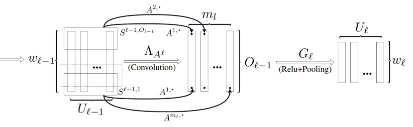
Figure 1: Illustration of architecture for one layer

Notation	Meaning
$G_{l}$	Activation + pooling at layer $l$
$A^{l}$	Filter matrix at layer $l$
$\Lambda_{A^{l}}$	Convolution operation relative to filter matrix $A^{l}$
$\tilde{A}^{l}$	Matrix representing $\Lambda_{A^{l}}$ (Has repeated weights in conv. net)
$O_{l}$	Number of convolutional patches at layer $l$
$m_{l}$	# of channels at layer $l$ before nonlinearity
	(=# of output channels at layer $l-1$)
$\gamma$	Classification margin
$S^{l,o}$	$o^{th}$ convolutional patch at layer $l$
$w_{l}$	Number of spatial dimensions at layer $l$ (No pooling $\implies$ $w_{l}=O_{l-1}$)
$U_{l}$	Number of channels after nonlinearity
$\rho_{l}$	Lipschitz constant of $G_{l}$
$W_{l}=U_{l}w_{l}$	Width (after pooling) at layer $l$
$W=\max_{l}W_{l}$	Maximum network width (after any pooling)
$\bar{W}=\max_{l}O_{l-1}m_{l}$	Maximum network width (before any pooling)
$\mathcal{W}$	Total number of parameters
$d_{l}$	Size of convolutional patches corresponding to the operation $\Lambda_{A^{l}}$
$|{\kern 0.8pt\raise 1.5pt\hbox{\bf.}\kern 0.8pt}|_{\infty,l}$	Max $l^{2}$ norm of a pixel across channels
$|{\kern 0.8pt\raise 1.5pt\hbox{\bf.}\kern 0.8pt}|_{l}$	Max $l^{2}$ norm of a convolutional patch (across channels)

Table 1: Table of notations for quick reference

Some key aspects of our proofs and general results rely on using the correct norms in activation spaces. On each activation space $\mathbb{R}^{w_{l}\times U_{l}}$, we will make use of the following three norms:

1. The $l^{\infty}$ norm: $|x|_{\infty}=\sup_{u\in\{1,\ldots,w_{l}\}\times\{1,\ldots,U_{l}\}}|x_{u}|$

2. The $|{\kern 0.8pt\raise 1.5pt\hbox{\bf.}\kern 0.8pt}|_{l}$ norm: $|x|_{l}=\sup_{o\leq O_{l}}\sqrt{\sum_{i\leq O_{l}}x_{i}^{2}}$, i.e. the maximum $l^{2}$ norm of a single convolutional patch.

3. The $|{\kern 0.8pt\raise 1.5pt\hbox{\bf.}\kern 0.8pt}|_{\infty,l}$ norm: $|x|_{\infty,l}=\sup_{o\leq w_{l}}\sqrt{\sum_{k\leq U_{l}}x_{o,k}^{2}}$, the maximum $l^{2}$ norm of a single pixel viewed as a vector over channels.

Remark 1.

In covering number arguments, we will use the same notation to refer to the norms on (activation,input) space induced by the above norms after taking a supremum over inputs.

Main result with Global Lipschitz bounds

Both of the results in the Section "contributions in a Nutshell" follow from the following result.

Theorem 7.

Assume that pooling does not occur over different channels, with probability $\geq 1-\delta$, every network $F_{\mathcal{A}}$ with weight matrices $\mathcal{A}=\{A^{1},A^{2},\ldots,A^{L}\}$ and every margin $\gamma>0$ satisfy:

$$\mathbb{P}\left(\operatorname*{arg\,max}_{j}(F_{\mathcal{A}}(x)_{j})\neq y\right)\leq\widehat{R}_{\gamma}(F_{\mathcal{A}})$$

$$\quad\quad+\widetilde{\mathcal{O}}\left(\frac{(R_{\mathcal{A}}+L)}{\sqrt{n}}\log(\bar{W})+\sqrt{\frac{\log(1/\delta)}{n}}\right),$$ (10)

where $W$ is the maximum number of neurons in a single layer (after pooling) and $R_{\mathcal{A}}:=$

$$\bigg{[}\sum_{l=1}^{L-1}\left(B_{l-1}(X)\|A^{l}-M^{l}\|_{2,1}\max_{\tilde{l}>l}\frac{\rho_{l\rightarrow\tilde{l}}}{B_{\tilde{l}}(X)}\right)^{2/3}+\left(\frac{B_{L-1}(X)}{\gamma}\|A^{L}-M^{L}\|_{\operatorname{Fr}}\right)^{2/3}\bigg{]}^{3/2},$$

where for any layer $l_{1}$, $B_{l_{1}}(X):=\max_{i}\left|F^{0\rightarrow l_{l}}(x_{i})\right|_{l_{1}}$denotes the maximum $l^{2}$ norm of any convolutional patch of the layer $l_{1}$ activations, over all inputs. $B_{L}(X)=\gamma$.

Here $\rho_{l_{1}\rightarrow l_{2}}$ is the Lipschitz constant of the map $F^{l_{1}\rightarrow l_{2}}$ with respect to the norms $|{\kern 0.8pt\raise 1.5pt\hbox{\bf.}\kern 0.8pt}|_{\infty,l_{1}}$ and $|{\kern 0.8pt\raise 1.5pt\hbox{\bf.}\kern 0.8pt}|_{l_{2}}$

Appendix B The one layer case

A key aspect of the proof is that we can use proposition 4 to obtain an $L^{\infty}$-covering of the map represented by a convolutional layer. Indeed, by viewing each (sample, convolutional patch, output channel) trio as an individual data point, we can, for each $\epsilon$, find $\mathcal{N}_{\epsilon}$ filters $f_{1},\ldots,f_{\mathcal{N}_{\epsilon}}$ with $\|f_{i}\|_{Fr}\leq a\quad\forall i$ such for any convolutional map represented by the filter $f$ (with $\|f\|_{Fr}\leq a$), there exists a $u_{f}\in\{1,2,\ldots,\mathcal{N}_{\epsilon}\}$ such that for any input $x_{i}$, any convolutional patch $S$, and any output channel $j$, the outputs of $f$ and $f_{u_{f}}$ corresponding to this (input, patch, channel) combination differ by less than $\epsilon$. More precisely, we can now prove Proposition 5

Proof of proposition 5.

This follows immediately from Lemma 4 applied to the $nmU$ data points in $\mathbb{R}^{d\times m}$ (considered as a simple vector space with the Hadamard product used as the scalar product) defined by, for all $\delta\in\{1,2,\ldots,m\}\times\{1,2,\ldots,d\}$, $(x_{u,i,j})_{\delta}=(X^{u}_{j})_{\delta_{2}}$ for $\delta_{1}=i$ and $(x_{u,i,j})_{\delta}=0$ otherwise, and the function class

$$\{F_{A}:\mathbb{R}^{d\times m}\rightarrow\mathbb{R}:x\mapsto x\odot A;\|A\|_{2}\leq a\},$$

where $\odot$ denotes the Hadamard product.

∎

Before we proceed, we will need the following Proposition:

Proposition 8 (cf. (Anthony and Bartlett 2002; Bartlett and Shawe-taylor 1998; Pisier 1980-1981)).

Let $B_{\beta}$ denote the ball of radius $\beta$ in $\mathbb{R}^{d}$ with respect to the $L^{1}$ norm. We have

$$\log\left(\mathcal{N}(B_{\beta},\epsilon,\|{\kern 0.8pt\raise 1.5pt\hbox{\bf.}\kern 0.8pt}\|_{2})\right)\leq\left\lceil\frac{\beta^{2}}{\epsilon^{2}}\right\rceil\log(2d)$$ (11)

Proof.

Wlog, $\beta=1$. Let $e_{1},\ldots,e_{d}$ denote the standard basis in $\mathbb{R}^{d}$, we will show that for any integer $k\in\mathbb{N}$ and any $a=(a_{1},a_{2},\ldots,a_{d})\in\mathbb{R}_{+}^{d}$ with $\sum_{i}a_{i}\leq 1$, there exists $(k_{1},k_{2},\ldots,k_{d})$ with $k_{i}\in\mathbb{N}$ such that $\kappa:=\sum_{i=1}^{d}e_{i}\frac{k_{i}}{k}$ satisfies

$$\|\kappa-a\|_{2}^{2}\leq\frac{1}{k}.$$

Let $(W_{1},\ldots,W_{k})$ be $k$ iid random variables with $\mathbb{P}(W_{1}=e_{i})=a_{i}$. Define $W=\frac{1}{k}\sum_{i=1}^{k}W_{i}$. We have $\mathbb{E}(W)=\mathbb{E}(W_{1})=\sum_{i=1}^{d}a_{i}e_{i}=a$. Thus we have

$$\mathbb{E}(\|W-a\|_{2}^{2}) =\frac{1}{k^{2}}\mathbb{E}\left(\sum_{i=1}^{k}\|a-W_{i}\|^{2}+\sum_{i\neq j}\langle a-W_{i},a-W_{j}\rangle\right)$$

$$=\frac{1}{k^{2}}\mathbb{E}\left(\sum_{i=1}^{k}\|a-W_{i}\|^{2}\right)=\frac{1}{k}\mathbb{E}\left(\|a-W_{1}\|^{2}\right)=\frac{1}{k}\left(\mathbb{E}(\|W_{1}\|^{2})-\|a\|^{2}\right)$$

$$\leq\frac{1}{k}\mathbb{E}(\|W_{1}\|^{2})=\frac{1}{k}.$$ (12)

By the probabilistic method, it follows that there is a choice $(k_{1},k_{2},\ldots,k_{d})$ such that $\|\kappa-a\|_{2}^{2}\leq\frac{1}{k},$ as expected.

It follows that one can find a cover of the ball $B_{\beta}$ with size $\mathcal{N}$, where $\mathcal{N}$ is the number of choices of $(k_{1},k_{2},\ldots,k_{d})$ with $k_{i}\in\mathbb{Z}$ and $\sum_{i=1}^{d}|k_{i}|=k$ and $k=\lceil\frac{\beta^{2}}{\epsilon^{2}}\rceil$. There are $2^{d}\left(\begin{array}[]{ccc}d+k-1\\ d-1\end{array}\right)\leq(2d)^{k}$ such choices. The result follows.

∎

With this in our toolkit, we can prove the extention of the one layer case to the $L^{2,1}$ norm with an extra covering umber argument:

Proof of Proposition 6.

First, note that the case $m=1$ follows from Proposition 5 (also with $m=1$).

Thus any set of $m$ positive real numbers $a=(a_{1},a_{2},\ldots,a_{m})$ and any $(\epsilon_{1},\epsilon_{2},\ldots,\epsilon_{m})$ with $\epsilon_{i}\leq\epsilon$ for all $i$, we can find covers $\mathcal{C}_{i}\subset\{A\in\mathbb{R}^{d}:\|A\|_{2}\leq a_{i}\}$ such that for all $A_{1},A_{2},\ldots,A_{m}\in\mathbb{R}^{d}$ such that $\|A_{i}\|_{2}\leq a_{i}\quad\forall i\leq m$, there exist $\bar{A}_{1},\bar{A}_{2},\ldots,\bar{A}_{m}\in\mathbb{R}^{d}$ such that $\|\bar{A}_{i}\|_{2}\leq a_{i}\quad\forall i\leq m$ and $\|XA_{i}-X\bar{A}_{i}\|_{\infty}\leq\epsilon_{1}$, and for all $i$, $\log(\#\mathcal{C}_{i})\leq\frac{36a_{i}^{2}b^{2}}{\epsilon_{i}^{2}}\log_{2}\left[\left(\frac{8a_{i}b}{\epsilon}+6\right)nU+1\right]$ (since $\epsilon_{i}\leq\epsilon$).

Writing $a=\sum_{i=1}^{m}a_{i}$, the cardinality of $\mathcal{C}_{(a_{1},a_{2},\ldots,a_{m})}=\mathcal{C}_{1}\times\mathcal{C}_{2},\ldots\times\mathcal{C}_{m}$ is bounded above by

$$36b^{2}\log_{2}\left[\left(\frac{8ab}{\epsilon}+6\right)nU+1\right]\sum_{i=1}^{m}\frac{a_{i}^{2}}{\epsilon_{i}^{2}}.$$ (13)

and the product cover is an $\epsilon$ cover of $\{XA:A\in\mathbb{R}^{d\times m},\|A_{{\kern 0.8pt\raise 1.5pt\hbox{\bf.}\kern 0.8pt},i}\|_{2}\leq a_{i}\forall i\}$ with respect to the $\|{\kern 0.8pt\raise 1.5pt\hbox{\bf.}\kern 0.8pt}\|_{*}$ norm, where $\epsilon^{2}=\sum_{i=1}^{m}\epsilon_{i}^{2}$.

Applying the above to $3\epsilon/4$ and calculating the Lagrangian to optimize over the $\epsilon_{i}$’s, we obtain the condition $\left(\frac{-2a_{i}^{2}}{\epsilon^{3}}\right)\propto 2\epsilon_{i}$, which yields $\epsilon_{i}=(3/4)\epsilon\frac{\sqrt{a_{i}}}{\sum a_{i}}=\epsilon\sqrt{a_{i}}/a$, which pluggind back into formula (13), yields,

$$\log(\#(\mathcal{C}_{1}\times\mathcal{C}_{2},\ldots,\mathcal{C}_{m})) \leq 36\frac{a^{2}b^{2}}{(3/4)^{2}\epsilon^{2}}\log_{2}\left[\left(\frac{8ab}{\epsilon}+7\right)nU\right]$$ (14)

$$\leq 64\frac{a^{2}b^{2}}{\epsilon^{2}}\log_{2}\left[\left(\frac{8ab}{\epsilon}+7\right)nU\right]$$ (15)

Of course, we do not know in advance the choice of $(a_{1},\ldots,a_{m})$ such that $\sum_{i=1}^{m}a_{i}=a$, so we must take extra steps to make the cover post hoc with respect to this choice. To do this we can choose the set $\mathcal{D}$ to be an $\epsilon/4b$ cover of $(a_{1},\ldots,a_{m}):\sum_{i=1}^{m}a_{i}=a$ with respect to the $L^{1}$ norm. By Proposition 8, we can ensure $\#(\mathcal{D})\leq\left\lceil 16a^{2}b^{2}/\epsilon^{2}\right\rceil\log(2m)\leq 64a^{2}b^{2}/\epsilon^{2}\log(m)$ (since we can assume $m\geq 2$ and wlog $16a^{2}b^{2}/\epsilon^{2}\geq 1$).

Clearly, the cardinality of the union $\cup_{a\in\mathcal{D}}\mathcal{C}_{1}\times\ldots\times\mathcal{C}_{m}$ is bounded by

$$\frac{64a^{2}b^{2}}{\epsilon^{2}}\log_{2}\left[\left(\frac{8ab}{\epsilon}+7\right)mnU\right],$$

so we only need to show that it constitutes an $\epsilon$ cover of $\{XA:A\in\mathbb{R}^{d\times m},\|A\|_{2,1}\leq a\}$. To see this, let $A\in\mathbb{R}^{d\times m}$ be given with $\|A\|_{2,1}\leq a$. Pick $(a_{1},a_{2},\ldots,a_{m})$ to be the closest element of $\mathcal{D}$ to $(\|A_{{\kern 0.8pt\raise 1.5pt\hbox{\bf.}\kern 0.8pt},1}\|_{2},\|A_{{\kern 0.8pt\raise 1.5pt\hbox{\bf.}\kern 0.8pt},2}\|_{2},\ldots,\|A_{{\kern 0.8pt\raise 1.5pt\hbox{\bf.}\kern 0.8pt},m}\|_{2})$ in terms of the $L^{\infty}$ norm. Then pick the element $\tilde{A}$ of $\mathcal{C}_{(a_{1},a_{2},\ldots,a_{m})}$ closest to $\bar{A}\in\mathbb{R}^{d\times m}$ defined by, $\forall i$, $\bar{A}_{{\kern 0.8pt\raise 1.5pt\hbox{\bf.}\kern 0.8pt},i}=A_{{\kern 0.8pt\raise 1.5pt\hbox{\bf.}\kern 0.8pt},i}$ if $\|A_{{\kern 0.8pt\raise 1.5pt\hbox{\bf.}\kern 0.8pt},i}\|_{2}\leq a_{i}$ and $\bar{A}_{{\kern 0.8pt\raise 1.5pt\hbox{\bf.}\kern 0.8pt},i}=\frac{a_{i}}{\|A_{{\kern 0.8pt\raise 1.5pt\hbox{\bf.}\kern 0.8pt},i}\|_{2}}A_{{\kern 0.8pt\raise 1.5pt\hbox{\bf.}\kern 0.8pt},i}$ otherwise. Clearly we have $\|XA-X\tilde{A}\|_{*}\leq\|XA-X\bar{A}\|_{*}+\|X\bar{A}-X\tilde{A}\|_{*}\leq\epsilon/5+4\epsilon/5=\epsilon$, which completes the proof.

∎

As a corollary of the above, we are now in a position to prove the one layer case.

Corollary 9.

Let $n,O,m,w,U$ be natural numbers, let $G:\mathbb{R}^{O}\times\mathbb{R}^{m}\rightarrow\mathbb{R}^{w}\times\mathbb{R}^{U}$ be $\rho$-Lipschitz with respect to the $|{\kern 0.8pt\raise 1.5pt\hbox{\bf.}\kern 0.8pt}|_{*}$ norms defined by $|x|_{*}=\sup_{i\in\{1,2\ldots,O\}}\sqrt{\sum_{j=1}^{m}x_{ij}^{2}}$ and $|x|_{*}=\sup_{i\in\{1,2\ldots,w\}}\sqrt{\sum_{j=1}^{U}x_{ij}^{2}}$ for $x\in\mathbb{R}^{O}\times\mathbb{R}^{m}$ and $x\in\mathbb{R}^{w}\times\mathbb{R}^{U}$ respectively (for instance, a combination of purely spacial pooling and elementwise relu satisfies this condition with $\rho=1$). We also write $|{\kern 0.8pt\raise 1.5pt\hbox{\bf.}\kern 0.8pt}|_{*}$ for the norm $\sup_{i\leq n}|X_{i,{\kern 0.8pt\raise 1.5pt\hbox{\bf.}\kern 0.8pt}}|_{*}$ for $X\in\mathbb{R}^{n}\times\mathbb{R}^{w}\times\mathbb{R}^{U}$ or $X\in\mathbb{R}^{n}\times\mathbb{R}^{O}\times\mathbb{R}^{m}$. For any $X\in\mathbb{R}^{n\times O\times d}$ such that $\|X^{i,o,{\kern 0.8pt\raise 1.5pt\hbox{\bf.}\kern 0.8pt}}\|_{2}^{2}\leq b^{2}$ ($\forall i,o$), we have for any fixed reference matrix $M$:

$$\log\mathcal{N}\left(\left\{G(XA):A\in\mathbb{R}^{d\times m},\|A-M\|_{2,1}\leq a\right\},\epsilon,|{\kern 0.8pt\raise 1.5pt\hbox{\bf.}\kern 0.8pt}|_{*}\right)\leq\frac{64a^{2}b^{2}}{\epsilon^{2}\rho^{2}}\log_{2}\left(\frac{8abnmO}{\epsilon\rho}+7Omn\right)$$ (16)

Appendix C Generalisation bound for fixed norm constraints

Once the one layer case is taken care of, we will now need to chain the covering number bounds of each layer, taking care to control the excess $|{\kern 0.8pt\raise 1.5pt\hbox{\bf.}\kern 0.8pt}|$ norms at each intermediary layer. To this effect, we have the following Proposition.

Proposition 10.

Let $L$ be a natural number and $a_{1},\ldots,a_{L}>0$ be real numbers. Let $\mathcal{V}_{0},\mathcal{V}_{1},\ldots,\mathcal{V}_{L}$ be $L+1$ vector spaces each endowed with two norms $|{\kern 0.8pt\raise 1.5pt\hbox{\bf.}\kern 0.8pt}|_{\infty,l}$ and $|{\kern 0.8pt\raise 1.5pt\hbox{\bf.}\kern 0.8pt}|_{l}$ for $0\leq l\leq L$. Let $B_{1},B_{2},\ldots,B_{L}$ be $L$ vector spaces with norms $\|{\kern 0.8pt\raise 1.5pt\hbox{\bf.}\kern 0.8pt}\|_{1},\|{\kern 0.8pt\raise 1.5pt\hbox{\bf.}\kern 0.8pt}\|_{2},\ldots,\|{\kern 0.8pt\raise 1.5pt\hbox{\bf.}\kern 0.8pt}\|_{L}$ and $\mathcal{B}_{1},\mathcal{B}_{2},\ldots,\mathcal{B}_{L}$ be the balls of radii $a_{1},a_{2},\ldots,a_{L}$ in the spaces $B_{1},B_{2},\ldots,B_{L}$ with the norms $\|{\kern 0.8pt\raise 1.5pt\hbox{\bf.}\kern 0.8pt}\|_{1},\|{\kern 0.8pt\raise 1.5pt\hbox{\bf.}\kern 0.8pt}\|_{2},\ldots,\|{\kern 0.8pt\raise 1.5pt\hbox{\bf.}\kern 0.8pt}\|_{L}$ respectively.

Suppose also that for each $l\in\{1,2,\ldots,L\}$ we are given an operator $F^{l}:\mathcal{V}_{l-1}\times B_{l}\rightarrow\mathcal{V}_{l}:(x,A)\rightarrow F^{l}_{A}(x)$, continuous with respect to the norms $\|{\kern 0.8pt\raise 1.5pt\hbox{\bf.}\kern 0.8pt}\|_{l}$ and $|{\kern 0.8pt\raise 1.5pt\hbox{\bf.}\kern 0.8pt}|_{l}$. For each $l_{1},l_{2}$ with $l_{2}>l_{1}$ and each $\mathcal{A}^{l_{1},l_{2}}=(A^{l_{1}+1},\ldots,A^{l_{2}})\in\mathcal{B}^{l_{1},l_{2}}:=\mathcal{B}_{l_{1}+1}\times\mathcal{B}_{l_{1}+2}\times\ldots\mathcal{B}_{l_{2}}$, let us define

$$F^{l_{1}\rightarrow l_{2}}_{\mathcal{A}^{l_{1},l_{2}}}:\mathcal{V}_{l_{1}}\rightarrow\mathcal{V}_{l_{2}}:x\rightarrow F^{l_{1}\rightarrow l_{2}}_{\mathcal{A}^{l_{1},l_{2}}}(x)=F^{l_{2}}_{A^{l_{2}}}\circ\ldots\circ F^{l_{1}}_{A^{l_{1}}}(x),$$

for all $l$, $\mathcal{F}^{l}_{\mathcal{A}^{L}}=F^{0\rightarrow l}_{\mathcal{A}^{L}}$ and $\mathcal{F}_{\mathcal{A}}=\mathcal{F}^{L}_{\mathcal{A}}.$

For each $\mathcal{A}^{L}=(A^{1},A^{2},\ldots,A^{L})\in\mathcal{B}^{L}:=\mathcal{B}_{1}\times\mathcal{B}_{2}\times\ldots,\mathcal{B}_{L}$, and for each $l\in\{1,2,\ldots,L\}$, the (worst case) Lipschitz constant of $F^{l_{1}\rightarrow l_{2}}$ with respect to the norms $\|{\kern 0.8pt\raise 1.5pt\hbox{\bf.}\kern 0.8pt}\|_{\infty,l_{1}}$ and $|{\kern 0.8pt\raise 1.5pt\hbox{\bf.}\kern 0.8pt}|_{l_{2}}$ is denoted by $\rho^{\mathcal{A}}_{l_{1}\rightarrow l_{2}}$.

We suppose the following conditions are satisfied:

For all $l\in\{1,2,\ldots,L\}$, all $b>0$, all $Z1,Z_{2},\ldots,Z_{n}\in\mathcal{V}_{l-1}$ such that $|Z_{i}|_{l-1}\leq b\quad\forall i$ and all $\epsilon>0$, there exists a subset $\mathcal{C}_{l}(b,Z,\epsilon)\subset\mathcal{B}_{l}$ such that

$$\log(\#\left(\mathcal{C}_{l}(b,Z,\epsilon)\right))\leq\frac{C_{l,\epsilon,n}a_{l}^{2}b^{2}}{\epsilon^{2}},$$ (17)

where $C_{l,\epsilon,n}$ is some function of $l,\epsilon,n,$ and, for all $A\in\mathcal{B}_{l}$, there exists an $\bar{A}\in\mathcal{C}_{l}(b,\epsilon)$ such that

$$\left|F^{l}_{A}(Z)-F^{l}_{\bar{A}}(Z)\right|_{\infty,l}\leq\epsilon\quad\quad\forall i.$$ (18)

For any $0<\epsilon<1$, any $b=(b_{0},b_{1},b_{2},\ldots,b_{L})$ with $b_{l}\geq 1\quad\forall l$ and $b_{L}=1$, any set of positive number $\rho_{l+}$ (for $l\leq L$) and for any $x_{1},\ldots,x_{n}\in\mathcal{V}_{0}$ such that $|x_{i}|_{0}\leq b_{0}\quad\forall i$, there exists a subset $\mathcal{C}_{\epsilon,b,n}$ of $\mathcal{B}^{L}$ such that for all $\mathcal{A}=(A^{1},A^{2},\ldots,A^{L})\in\mathcal{B}:=\mathcal{B}^{L}$ such that $\rho^{\mathcal{A}}_{l_{1}\rightarrow l_{2}}\leq\rho_{l_{1}}b_{l_{2}}\quad\forall l_{2}\geq l_{1}$, there exists a $\bar{\mathcal{A}}\in\mathcal{C}_{\epsilon,b,X}$ such that, for any $i$ such that $\left|\mathcal{F}^{l}_{\mathcal{A}}(x_{i})\right|_{l}\leq b_{l}\quad\forall l$, we have

$$\left|F^{0\rightarrow l}_{\mathcal{A}^{l}}(x_{i})-F^{0\rightarrow l}_{\bar{\mathcal{A}}^{l}}(x_{i})\right|_{l} \leq\epsilon b_{l}\quad\quad(\forall l<L,\forall i)\quad\text{and}$$

$$\left|\mathcal{F}^{l}_{\bar{\mathcal{A}}}(X)\right|_{l} \leq 2b_{l}.$$ (19)

Furthermore, we have

$$\log\#(\mathcal{C}_{\epsilon,b,X}) \leq 4\left[\sum_{l=1}^{L}\left(\frac{C_{l,\epsilon}^{\frac{1}{2}}a_{l}b_{l-1}\rho_{l}}{\epsilon}\right)^{\frac{2}{3}}\right]^{3}\leq 4\frac{L^{2}}{\epsilon^{2}}\sum_{l=1}^{L}\left(\frac{C_{l,\epsilon}^{\frac{1}{2}}a_{l}b_{l-1}\rho_{l}}{\epsilon}\right)^{2}.$$ (20)

Proof.

For $l=1,\ldots,L$, let $\epsilon_{l}=\frac{\epsilon\alpha_{l}}{\rho_{l}}$, where the $\alpha_{l}>0$ will be determined later satisfying $\sum_{l=1}^{L}\alpha_{l}=1$.

For any $X=(x_{1},\ldots,x_{n})$, we define the covers $\mathcal{D}_{l}\subset\mathcal{B}_{l}$ for $l\leq L$ by induction by $\mathcal{D}_{l}=\cup_{\mathcal{A}\in\mathcal{D}_{1}\times\ldots\times\mathcal{D}_{l-1}}\mathcal{C}(2b_{l},\{F^{0\rightarrow l-1}_{\mathcal{A}}(x_{i}):i\leq n\},\epsilon_{l})$. Let us write also $\mathcal{D}:=\mathcal{D}_{1}\times\mathcal{D}{2}\ldots\mathcal{D}_{L}$, and let us write $d_{l}$ for the cardinality of $\mathcal{D}_{l}$. We prove the equations (18) by induction. The case $l=1$ follows directly from the definition of $\mathcal{D}_{1}$ and the assumption on the $x_{i}$’s. For the induction case, let us assume the inequalities hold for each $u\leq l-1$. We have for any $j\leq n$,

$$\left|F^{0\rightarrow l}_{\mathcal{A}}(x_{j})-F^{0\rightarrow l}_{\bar{\mathcal{A}}}(x_{j})\right|_{l} \leq\sum_{i=1}^{L}\left|F^{0\rightarrow l}_{\left(\bar{A}_{1},\bar{A}_{2},\ldots,\bar{A}_{i-1},A_{i},\ldots,A_{l}\right)}(x_{j})-F^{0\rightarrow l}_{\left(\bar{A}_{1},\bar{A}_{2},\ldots,\bar{A}_{i},A_{i+1},\ldots,A_{i}\right)}(x_{j})\right|_{l}$$

$$\leq\sum_{i=1}^{l}\rho^{\mathcal{A}}_{i\rightarrow l}\left|F^{0\rightarrow i}_{(\bar{A}_{1},\bar{A}_{2},\ldots,\bar{A}_{i-1},A_{i})}(x_{j})-F^{0\rightarrow i}_{\left(\bar{A}_{1},\bar{A}_{2},\ldots,\bar{A}_{i}\right)}(x_{j})\right|_{i}$$

$$\leq\sum_{i=1}^{l}\rho^{\mathcal{A}}_{i\rightarrow l}\frac{\epsilon\alpha_{i}}{\rho_{i}}\leq\sum_{i=1}^{l}\rho^{\mathcal{A}}_{i\rightarrow l}\frac{\epsilon\alpha_{i}}{\rho^{\mathcal{A}}_{i\rightarrow l}/b_{l}}\leq\epsilon b_{l},$$ (21)

where at the first line, we have used the triangle inequality, at the second line, the definition of $\rho_{i\rightarrow l}$, and at the last line, the fact that $\rho^{\mathcal{A}}_{l_{1}\rightarrow l_{2}}\leq\rho_{l_{1}}\quad\forall l_{2}\geq l_{1}$. Now, by the triangle inequality, we obtain:

$$\left|F^{0\rightarrow l}_{\bar{\mathcal{A}}}(x_{j})\right|_{l}\leq\left|F^{0\rightarrow l}_{\mathcal{A}}(x_{j})\right|_{l}+\epsilon b_{l}\leq 2b_{l},$$ (22)

which concludes the proof by induction.

To finish the proof of the proposition, we just need to calculate the bound on the caridinality of $\mathcal{D}$:

$$\log(\#(\mathcal{D})) =\sum_{l=1}^{L}\log(\#(\mathcal{D}_{l}))=\sum_{l=1}^{L}\log(d_{l})$$

$$\leq\sum_{l=1}^{L}4\frac{C_{l,\epsilon}a_{l}^{2}b_{l-1}^{2}}{\epsilon_{l}^{2}}=\sum_{l=1}^{L}4\frac{C_{l,\epsilon}a_{l}^{2}b_{l-1}^{2}}{(\frac{\alpha_{l}\epsilon}{\rho_{l}})^{2}}$$

$$=\frac{4}{\epsilon^{2}}\sum_{l=1}^{L}\frac{C_{l,\epsilon}a_{l}^{2}b_{l-1}^{2}\rho_{l}^{2}}{\alpha_{l}^{2}}.$$ (23)

Optimizing over the $\alpha_{l}$’s subject to $\sum_{l=1}^{L}\alpha_{l}=1$, we find the Lagrangian condition

$$\left(-\frac{2C_{l,\epsilon}a_{l}^{2}\rho_{l}^{2}}{\alpha_{l}^{3}}\right)_{l=1}^{L}\propto(1)_{l=1}^{L},$$

yielding

$$\alpha_{l}=\frac{(\sqrt{C_{l,\epsilon}}a_{l}\rho_{l})^{\frac{2}{3}}}{\sum_{i=1}^{L}(\sqrt{C_{i}}a_{i}\rho_{i})^{\frac{2}{3}}}.$$

Substituting back into equation (C), we obtain

$$\log\#\left(\{F_{\mathcal{A}}(X):\mathcal{A}\in\mathcal{D}\}\right) \leq 4\left[\sum_{i=1}^{L}\left(\frac{\sqrt{C_{i}}a_{i}b_{i-1}\rho_{i}}{\epsilon}\right)^{\frac{2}{3}}\right]^{2}\sum_{l=1}^{L}\left(\frac{\sqrt{C_{l,\epsilon}}a_{l}b_{l-1}\rho_{l}}{\epsilon}\right)^{2-4/3}$$

$$=\frac{4}{\epsilon^{2}}\left[\sum_{i=1}^{L}\left(\sqrt{C_{i}}a_{i}b_{i-1}\rho_{i}\right)^{\frac{2}{3}}\right]^{3},$$

as expected. The last inequality follows from Jensen’s inequality.

∎

The next step is to use the above, together with the classic Rademacher theorem 25 and Dudley’s Entropy integral, to obtain a result about large margin multi-class classifiers.

Theorem 11.

Suppose we have a $K$ class classification problem and are given $n$ i.i.d. observations $(x_{1},y_{1}),(x_{2},y_{2}),\ldots,(x_{n},y_{n})\in\mathbb{R}^{U_{0}\times w_{0}}\otimes\{1,2,\ldots,K\}$ drawn from our ground truth distribution $(X,Y)$, as well as a fixed architecture as described in Section A, where we assume the last layer is fully connected and has width $K$ and corresponds to scores for each class. Suppose also that with probability one $|x|_{0}\leq b_{0}$. Suppose we are given numbers $a_{1},a_{2},\ldots,a_{L}$, $\beta=(b_{0},b_{1},\ldots,b_{L}=\gamma)$ and $\rho_{l_{1}\rightarrow l_{2}}$ (for $l_{1},l_{2}\leq L$). For any $\delta>0$, with probability $>1-\delta$ over the draw of the training set, for any network $\mathcal{A}=(A^{1},A^{2},\ldots,A^{L})$ satisfying $\forall l:\|(A^{l})^{\top}\|_{2,1}\leq a_{l}\land\rho^{\mathcal{A}}_{l_{1}\rightarrow l_{2}}\leq\rho_{l_{1}\rightarrow l_{2}}$, we have

$$\mathbb{P}\left(\operatorname*{arg\,max}_{j\in\{1,2,\ldots,K\}}(F_{L}(x))_{j}\neq y\right)$$

$$\leq\frac{n-\#(I_{\beta,\gamma})}{n}+\frac{8}{n}+\frac{1536}{\sqrt{n}}R\left[\log_{2}(32\Gamma n^{2}+7\bar{W}n)\right]^{\frac{1}{2}}\log(n)+3\sqrt{\frac{\log(\frac{2}{\delta})}{2n}},$$ (24)

where

$$I=\left\{i\leq n:(f(x_{i}))_{y_{i}}-\max_{j\neq y_{i}}((f(x_{i}))_{j})>\gamma\land\forall l\leq L:\left|F^{0\rightarrow l}(x_{i})\right|_{l}\leq b_{l}\right\},$$

$$R^{2/3} :=\sum_{l=1}^{L}\left(a_{l}b_{l-1}\rho_{l+}\right)^{2/3},\quad\text{and}$$

$$\Gamma :=\max_{l=1}^{L}\left(b_{l-1}a_{l}O_{l-1}m_{l}\rho_{l+}\right),$$ (25)

$\rho_{l+}=\max_{i=l}^{L}\frac{\rho_{l\rightarrow i}}{b_{i}}.$

Proof.

As explained in the sketch in the main text, we apply the Rademacher theorem to the loss function:

$$l(x_{i},y_{i})=\max\left[\sup_{l=1}^{L-1}\lambda_{B_{l}}\left(\left|F^{0\rightarrow l}(x_{i})\right|_{l}-2B_{l}\right),\lambda_{\gamma}\left(\max_{j\neq y}(F_{\mathcal{A}}(x))_{j}-F_{\mathcal{A}}(x)_{y}\right)\right]$$ (26)

Writing $\mathcal{H}$ for the function class defined by $l(x,F^{\mathcal{A}}(x))$ for $F^{\mathcal{A}}$ satisfying the conditions of the Theorem, since $Y\mapsto\max_{j\neq y}(Y)_{j}-Y_{y}$ is $2$ Lipschitz with respect to the $l^{\infty}$ norm, and $l(x,y)=1$ for any $x$ such that there exists $l$ such that $|F^{0\rightarrow l}(x)|_{l}\geq 2b_{l}$, Propositions 10 and 9 guanrantee that the covering number of $\mathcal{H}$ satisfies

$$\log(\mathcal{N}(\mathcal{H},\epsilon)) \leq 4\times 64\times 2^{2}\left[\sum_{l=1}^{L}\left(\frac{a_{l}(2b_{l-1})}{\epsilon}\rho_{l+}\log_{2}\left(8\frac{a_{l}(2b_{l-1})nm_{l}O_{l-1}}{(\epsilon/\rho_{l+})}+7O_{l-1}m_{l}n\right)\right)^{2/3}\right]^{3}$$

$$\leq 2^{12}R^{2}\log_{2}(32\Gamma n/\epsilon+7\bar{W}n)$$ (27)

Applying the Rademacher Theorem 25, we now obtain

$$\mathbb{P}\left(\operatorname*{arg\,max}_{j\in\{1,2,\ldots,K\}}(F_{L}(x))_{j}\neq y\right)\leq\mathbb{E}\left(l(x,y)\right)$$

$$\leq\frac{\sum_{i=1}^{n}l(x_{i},y_{i})}{n}+3\sqrt{\frac{\log(\frac{2}{\delta})}{2n}}+2\hat{\operatorname{\mathfrak{R}}}_{n}(l(x,y))$$

$$\leq\frac{n-\#(I)}{n}+3\sqrt{\frac{\log(\frac{2}{\delta})}{2n}}+2\hat{\operatorname{\mathfrak{R}}}_{n}(l(x,y)).$$ (28)

Now, by Dudley’s Entropy integral 73 with $\alpha=\frac{1}{n}$, we have

$$\hat{\operatorname{\mathfrak{R}}}_{n}(l(x,y)) \leq 4\alpha+\frac{12}{\sqrt{n}}\int_{\alpha}^{1}\sqrt{\log\mathcal{N}(\mathcal{F}|S,\epsilon,\|{\kern 0.8pt\raise 1.5pt\hbox{\bf.}\kern 0.8pt}\|_{p})}$$

$$\leq\frac{4}{n}+\sqrt{R}\sqrt{2^{12}}\frac{12}{\sqrt{n}}\int_{\frac{1}{n}}^{1}\frac{\sqrt{\log_{2}(32\Gamma n/\epsilon+7\bar{W}n)}}{\epsilon}$$

$$\leq\frac{4}{n}+\sqrt{R}\frac{768}{\sqrt{n}}\sqrt{\log_{2}(32\Gamma n^{2}+7\bar{W}n)}\log(n)$$

Plugging this back into equation C, we obtain the desired result.

∎

Appendix D Proofs of post hoc result and asymptotic results

The next step from Theorem 11 to Theorem 7 is now mostly a question of applying classical techniques, namely, splitting the space of possible choices of parameters $(a_{1},\ldots,a_{L},b_{0},\ldots,b_{L},\gamma,\rho_{0\rightarrow 1},\ldots,)$ into different regions and using a union bound. The following Lemma summarizes the techniques in question:

Lemma 12.

Let $R_{\mathcal{N}}$ denote a random variable indexed some finite dimensional vector $\mathcal{N}$. Let $\gamma_{1}(\mathcal{N}),\ldots,\gamma_{l}(\mathcal{N}),N_{1}(\mathcal{N}),\ldots,N_{L}(\mathcal{N})$ be some (positive) statistics of $\mathcal{N}$. Suppose there exists a function $F:\mathbb{R}_{+}^{l\times L}\rightarrow\mathbb{R}$ which is monotonically decreasing in $\gamma_{i}$ for all $i\leq l$ and monotonically increasing in $N_{i}$ for $i\leq L$, such that the following statement holds:

For any $\gamma_{1},\ldots,\gamma_{l},N_{1},\ldots,N_{L}$, and for any $\delta>0$, with probability $>1-\delta$, we have that for any $\mathcal{N}$ such that $\gamma_{i}(\mathcal{N})\leq\gamma_{i}$ for all $i$ and $N_{i}(\mathcal{N})\leq N_{i}$ for all $i$,

$$R_{\mathcal{N}} \leq f(\gamma_{1},\ldots,\gamma_{l},N_{1},\ldots,N_{L})+C_{1}\sqrt{\frac{\log(1/\delta)}{C_{2}}},$$ (30)

for some constants $C_{1},C_{2}$.

For any fixed choice of $\beta_{1},\ldots,\beta_{L}$ and $\kappa_{1},\ldots,\kappa_{l}\in\mathbb{N}$, we have for any $\delta>0$ that with probability greater than $1-\delta$, for any $\mathcal{N}$,

$$R_{\mathcal{N}} \leq f(\min(\gamma_{1}(\mathcal{N})/2,\frac{1}{\kappa_{1}}),\ldots,\min(\gamma_{l}(\mathcal{N})/2,\frac{1}{\kappa_{l}}),N_{1}(\mathcal{N})+\beta_{1},\ldots,N_{L}(\mathcal{N})+\beta_{L})$$

$$+\frac{C_{1}}{\sqrt{C_{2}}}\sqrt{\log(1/\delta)+\sum_{i=1}^{l}\log(2\kappa_{i}(\mathcal{N})/\gamma_{i}(\mathcal{N}))+2\sum_{i=1}^{L}\log\left(2+\frac{N_{i}(\mathcal{N})}{\beta_{i}}\right)}.$$ (31)

Proof.

For any $j_{1},\ldots,j_{l},n_{1},\ldots,n_{L}\in\mathbb{N}$, define

$$\delta_{j_{1},\ldots,j_{l},n_{1},\ldots,n_{L}}=\frac{\delta}{\prod_{i=1}^{l}2^{j_{i}}\prod_{i=1}^{L}n_{i}(n_{i}+1)}.$$

Define $\gamma_{i}^{j_{i}}=\frac{\kappa_{i}}{2^{j_{i}}}$ and $N^{n_{i}}_{i}=n_{i}\beta_{i}$. By applying equation (30), we obtain that with probability $\geq 1-\delta_{j_{1},\ldots,j_{l},n_{1},\ldots,n_{L}}$,

$$R_{\mathcal{N}} \leq f(\gamma^{j_{1}}_{1},\ldots,\gamma^{j_{l}}_{l},N^{n_{1}}_{1},\ldots,N^{n_{L}}_{L})+C_{1}\sqrt{\frac{\log(1/\delta_{j_{1},\ldots,j_{l},n_{1},\ldots,n_{L}})}{C_{2}}},$$ (32)

Note that $\sum_{j_{1},\ldots,j_{l},n_{1},\ldots,n_{L}}\delta_{j_{1},\ldots,j_{l},n_{1},\ldots,n_{L}}=\delta$.

Thus, by a union bound, we obtain that with probability $\geq 1-\delta$, for any choice of $j_{1},\ldots,j_{l},n_{1},\ldots,n_{L}\in\mathbb{N}$, we have

$$R_{\mathcal{N}} \leq f(\gamma^{j_{1}}_{1},\ldots,\gamma^{j_{l}}_{l},N^{n_{1}}_{1},\ldots,N^{n_{L}}_{L})+C_{1}\sqrt{\frac{\log(1/\delta_{j_{1},\ldots,j_{l},n_{1},\ldots,n_{L}})}{C_{2}}}.$$ (33)

For any network $\mathcal{N}$, we can apply this for the choice of $j_{1},\ldots,j_{l}$ which are smallest whist still guaranteeing

$$\frac{1}{\gamma_{i}(\mathcal{N})}\leq\frac{1}{\gamma_{i}^{j_{i}}}=\frac{2^{j_{i}}}{\kappa_{i}},$$

and

$$N_{i}(\mathcal{N})\leq n_{i}\beta_{i}.$$

For this choice, we have $\gamma_{i}^{j_{i}}\geq\min(\gamma(\mathcal{N})/2,\frac{1}{\kappa_{i}}))$ for all $i\leq l$ and $N_{i}^{n_{i}}\leq N_{i}(\mathcal{N})+\beta_{i}$, thus by the properties of $f$,

$$f(\gamma^{j_{1}}_{1},\ldots,\gamma^{j_{l}}_{l},N^{n_{1}}_{1},\ldots,N^{n_{L}}_{L})$$

$$\leq f(\min(\gamma_{1}(\mathcal{N})/2,\frac{1}{\kappa_{1}}),\ldots,\min(\gamma_{l}(\mathcal{N})/2,\frac{1}{\kappa_{l}}),N_{1}(\mathcal{N})+\beta_{1},\ldots,N_{L}(\mathcal{N})+\beta_{L}).$$ (34)

Furthermore, we also have $2^{j_{i}}\leq 2\kappa_{i}/\gamma_{i}(\mathcal{N})$ and $n_{i}(n_{i}+1)\leq\left(1+\frac{N_{i}(\mathcal{N})}{\beta_{i}}\right)\left(2+\frac{N_{i}(\mathcal{N})}{\beta_{i}}\right)\leq\left(2+\frac{N_{i}(\mathcal{N})}{\beta_{i}}\right)$, and thus

$$C_{1}\sqrt{\frac{\log(1/\delta_{j_{1},\ldots,j_{l},n_{1},\ldots,n_{L}})}{C_{2}}}\leq\frac{C_{1}}{\sqrt{C_{2}}}\sqrt{\log(1/\delta)+\sum_{i=1}^{l}\log(2\kappa_{i}(\mathcal{N})/\gamma_{i}(\mathcal{N}))+2\sum_{i=1}^{L}\log\left(2+\frac{N_{i}(\mathcal{N})}{\beta_{i}}\right)}.$$ (35)

Plugging equations (D) and (35) back into equation (33) yields the desired result.

∎

Using this, we obtain the following:

Theorem 13.

Suppose we have a $K$ class classification problem and are given $n$ i.i.d. observations $(x_{1},y_{1}),(x_{2},y_{2}),\ldots,(x_{n},y_{n})\in\mathbb{R}^{U_{0}\times w_{0}}\otimes\{1,2,\ldots,K\}$ drawn from our ground truth distribution $(X,Y)$, as well as a fixed architecture as described in Section A, where we assume the last layer is fully connected and has width $K$ and corresponds to scores for each class. For any $\delta>0$, with probability $>1-\delta$ over the draw of the training set, for any network $\mathcal{A}=(A^{1},A^{2},\ldots,A^{L})$ we have

$$\mathbb{P}\left(\operatorname*{arg\,max}_{j\in\{1,2,\ldots,K\}}(F_{L}(x))_{j}\neq y\right)$$

$$\leq\frac{n-\#(I_{\beta,\gamma})}{n}+\frac{8}{n}+\frac{1536}{\sqrt{n}}R_{\mathcal{A}}\left[\log_{2}(32\Gamma n^{2}+7\bar{W}n)\right]^{\frac{1}{2}}\log(n)+3\sqrt{\frac{\log(\frac{2}{\delta})}{2n}}$$ (36)

$$+3\sqrt{\frac{1}{n}\sum_{l=1}^{L}\log\left(2+\frac{B_{l-1}(X)}{L}\right)+\log\left(2+\frac{\|(A-M)^{\top}\|_{2,1}}{L}\right)+\log\left(2+\frac{\rho^{\mathcal{A}}_{l+}}{L}\right)},$$ (37)

where

$$I=\left\{i\leq n:(f(x_{i}))_{y_{i}}-\max_{j\neq y_{i}}((f(x_{i}))_{j})>\gamma\land\forall l\leq L:\left|F^{0\rightarrow l}(x_{i})\right|_{l}\leq B_{l}(X)\right\},$$

$$R_{\mathcal{A}}^{2/3} :=\sum_{l=1}^{L}\left((\|(A-M)^{\top}\|_{2,1}+\frac{1}{L})(B_{l-1}(X)+\frac{1}{L}))(\rho^{\mathcal{A}}_{l+}+\frac{1}{L})\right)^{2/3},\quad\text{and}$$

$$\Gamma :=\max_{l=1}^{L}\left((B_{l-1}(X)+\frac{1}{L})(\|(A-M)^{\top}\|_{2,1}+\frac{1}{L})O_{l-1}m_{l}(\rho^{\mathcal{A}}_{l+}+\frac{1}{L})\right),$$ (38)

$\rho^{\mathcal{A}}_{l+}=\max_{i=l}^{L}\frac{\rho^{\mathcal{A}}_{l\rightarrow i}}{B_{i}(X)}.$

Here, $X$ denotes the design matrix containing the sample points, $B_{L}=\gamma>0$ is arbitrary and $B_{l}(X)$ for $l\leq L-1$ can be chosen arbitrarily so that $B_{l}(X)\geq 1$in a way that depends on $X$, with the choice $B_{l}(X)=\max\left(\max_{i\leq n}\left|F_{0\rightarrow l}^{\mathcal{A}}(x_{i})\right|_{l},1\right)$ yielding

$$I=\left\{i\leq n:(f(x_{i}))_{y_{i}}-\max_{j\neq y_{i}}((f(x_{i}))_{j})>\gamma\right\}.$$

Proof.

We split the space using Lemma 12 for the parameters $B_{0},B_{1},\ldots,B_{L-1}$, $\rho^{\mathcal{A}}_{l+}$. Note that the bound is increasing in all of those parameters, se we can treat them all as a "$N_{i}$"s from Lemma 12. Setting all the $k_{i}$’s to $L$ yields the result. Note that the dependence on $\gamma$ is hidden in the definition of $\rho^{\mathcal{A}}_{l+}$. The bound doesn’t go to zero as $\gamma$ as a result of the need to estimate the risk of intermediary activations being too large.

As explained in the main text, if one is willing to forgo the gains obtained from the sparsity of the connections inside the definition of $B_{l}$, then one can obtain bounds that scale like $1/\gamma$. ∎

Proof of Theorem 7.

This is simply a question of reducing to the $\tilde{O}$ notation. Note that $\log(n^{2})$, $\frac{1}{\sqrt{n}}$, $\Gamma$ are all $\tilde{O}(\frac{R_{\mathcal{A}}}{\sqrt{n}})$, and asymptotically, $\log_{2}(32\Gamma n^{2}+7\bar{W}n)\leq\log_{2}(32\Gamma n^{2})+\log_{2}(7\bar{W}n)$, thus we only have to take care of the last line. For this, note that each of the concerned log terms inside the square root are also $\tilde{O}(\frac{R_{\mathcal{A}}}{\sqrt{n}})$, yielding the result (with a factor of $\sqrt{R}$ from the sum).

∎

Similarly, in the case where the spectral norms are well controlled, we have the following result:

Theorem 14.

Suppose we have a $K$ class classification problem and are given $n$ i.i.d. observations $(x_{1},y_{1}),(x_{2},y_{2}),\ldots,(x_{n},y_{n})\in\mathbb{R}^{U_{0}\times w_{0}}\otimes\{1,2,\ldots,K\}$ drawn from our ground truth distribution $(X,Y)$, as well as a fixed architecture as described in Section A, where we assume the last layer is fully connected and has width $K$ and corresponds to scores for each class. For any $\delta>0$, with probability $>1-\delta$ over the draw of the training set, for any network $\mathcal{A}=(A^{1},A^{2},\ldots,A^{L})$ we have

$$\mathbb{P}\left(\operatorname*{arg\,max}_{j\in\{1,2,\ldots,K\}}(F_{L}(x))_{j}\neq y\right)$$

$$\leq\frac{n-\#(I_{\beta,\gamma})}{n}+\frac{8}{n}+\frac{3072}{\sqrt{n}}R_{\mathcal{A}}\left[\log_{2}(64\Gamma n^{2}+7\bar{W}n)\right]^{\frac{1}{2}}\log(n)+3\sqrt{\frac{\log(\frac{2}{\delta})}{2n}}+\sqrt{\log\left(\frac{2}{\gamma n}\right)}$$ (39)

$$+3\sqrt{\frac{1}{n}\sum_{l=1}^{L}\log\left(2+LB_{l-1}(X)\right)+\log\left(2+\|(A-M)^{\top}\|_{2,1}\right)+\log\left(2+L\|\tilde{A}\|_{\sigma^{\prime}}\right)},$$ (40)

where

$$I=\left\{i\leq n:(f(x_{i}))_{y_{i}}-\max_{j\neq y_{i}}((f(x_{i}))_{j})>\gamma\land\forall l\leq L:\left|F^{0\rightarrow l}(x_{i})\right|_{l}\leq B_{l}(X)\right\},$$

$$R_{\mathcal{A}}^{2/3} :=\sum_{l=1}^{L}\left((\|(A-M)^{\top}\|_{2,1}+\frac{1}{L})(B_{l-1}(X)+\frac{1}{L}))\max_{l^{\prime}}\frac{\prod_{i=l+1}^{l^{\prime}}(\|\tilde{A}\|_{\sigma^{\prime}}+\frac{1}{L})}{B_{l^{\prime}}(X)}\right)^{2/3},\quad\text{and}$$

$$\Gamma :=\max_{l=1}^{L}\left((B_{l-1}(X)+\frac{1}{L})(\|(A-M)^{\top}\|_{2,1}+\frac{1}{L})O_{l-1}m_{l}\max_{l^{\prime}}\frac{\prod_{i=l+1}^{l^{\prime}}(\|\tilde{A}\|_{\sigma^{\prime}}+\frac{1}{L})}{B_{l^{\prime}}(X)}\right).$$ (41)

Here, $X$ denotes the design matrix containing the sample points, $B_{L}=\gamma>0$ is arbitrary and $B_{l}(X)$ for $l\leq L-1$ can be chosen arbitrarily so that $B_{l}(X)\geq 1$ in a way that depends on $X$, with the choice $B_{l}(X)=\max\left(\max_{i\leq n}\left|F_{0\rightarrow l}^{\mathcal{A}}(x_{i})\right|_{l},1\right)$ yielding

$$I=\left\{i\leq n:(f(x_{i}))_{y_{i}}-\max_{j\neq y_{i}}((f(x_{i}))_{j})>\gamma\right\}.$$

Proof.

We apply theorems 11 and Lemma 12 for the parameters $\gamma,B_{0},\ldots,B_{L},a_{1},\ldots,a_{L},s_{1},s_{2},\ldots,s_{L}$ where $s_{i}$ is a bound on $\|\tilde{A}_{i}\|_{\sigma^{\prime}}$: note first that if $\|\tilde{A}_{i}\|_{\sigma^{\prime}}\leq s_{i}$ for all $i$, then $\rho^{\mathcal{A}}_{l_{1}\rightarrow l_{2}}\leq\prod_{l=l_{1}+1}^{l_{2}}\rho_{l}s_{i}$ for all $l_{1}\leq l_{2}$, and if furthermore $\gamma^{\mathcal{A}}\geq\bar{\gamma}$ and $B_{l}(X)\geq\bar{B}_{l}$, for all $l\leq L-1$, we have $\rho^{\mathcal{A}}_{l_{1}+}\leq\sqrt{l_{1}}\max_{l_{2}}\frac{\prod_{l=l_{1}+1}^{l_{2}}\rho_{l}s_{i}}{\bar{B}_{l_{2}}}$, with $\bar{B}_{L}=\bar{\gamma}$. Thus we can apply Lemma 12 with the $\beta_{i}=\frac{1}{L}$ and $\gamma$ being treated as a decreasing variable with $k=n$, to obtain the required result ($\bar{\gamma}\geq\gamma^{\mathcal{A}}/2$ and $\bar{B}_{l}\geq B_{l}/2$, furthermore, the case $\gamma\leq\frac{1}{2n}$ is trivial since the RHS is $\geq 1$ ).

∎

We can now proceed to the proof of theorem 3:

Proof.

The only difference between this proof and that of Theorem 7 is in the treatment of the sum of log terms at the last line. For this, note that $\|(A-M)^{\top}\|_{2,1}\leq\|(A)^{\top}\|_{2,1}+\|(M)^{\top}\|_{2,1}\leq\|(M)\|^{\top}_{2,1}+\sqrt{\bar{W}}\|(A)^{\top}\|_{2}\leq\|(M)^{\top}\|_{2,1}+\bar{W}\|A\|_{\sigma^{\prime}}\leq\|(M)^{\top}\|_{2,1}+\bar{W}^{3/2}\|A\|_{\sigma^{\prime}})$, thus

$\sqrt{\frac{1}{n}\sum_{l=1}^{L}\log\left(2+L\|(A-M)^{\top}\|_{2,1}\right)}$ is $\tilde{O}(\prod_{l=1}^{L}\|\tilde{A}\|_{\sigma^{\prime}}\rho_{l})$, which is $\tilde{O}(\frac{R_{\mathcal{A}}}{\sqrt{n}})$ as expected.

∎

Appendix E Simpler results with explicit norms

In this Section, we show slight variations of our bounds sticking closer to (Bartlett, Foster, and Telgarsky 2017) by only using norms involved at each individual layer or pair of layer. Theorem 3 follows from the theorems below. Whilst the results don’t seem to follow directly from the above, the treatment is extremely similar. Suppose we are given some norms $|{\kern 0.8pt\raise 1.5pt\hbox{\bf.}\kern 0.8pt}|_{\mathcal{L}_{l}}$ on the activation spaces and some norms $|{\kern 0.8pt\raise 1.5pt\hbox{\bf.}\kern 0.8pt}|_{\mathcal{L}_{l}^{*}}$ on the weight spaces such that $|{\kern 0.8pt\raise 1.5pt\hbox{\bf.}\kern 0.8pt}|_{\mathcal{L}_{l}}\leq|{\kern 0.8pt\raise 1.5pt\hbox{\bf.}\kern 0.8pt}|_{l}$ and the Lipschitz constant of $\Lambda_{l}(A)$ with respect to $|{\kern 0.8pt\raise 1.5pt\hbox{\bf.}\kern 0.8pt}|_{\mathcal{L}_{l-1}}$ and $|{\kern 0.8pt\raise 1.5pt\hbox{\bf.}\kern 0.8pt}|_{\mathcal{L}_{l}}$ is bounded by $|A|_{\mathcal{L}^{*}}$ and $|{\kern 0.8pt\raise 1.5pt\hbox{\bf.}\kern 0.8pt}|_{\infty,l}\leq\sqrt{k_{l}}|{\kern 0.8pt\raise 1.5pt\hbox{\bf.}\kern 0.8pt}|_{\mathcal{L}_{l}}$

Note that for any $s$, a simple argument on internal vs. external covering numbers shows that Theorem 9 can be adapted to yield a cover such that $\|\tilde{A}\|_{\sigma^{\prime}}\leq s$ for any $A$ in the cover, at the cost of a factor of $2$ in $\epsilon$.

We have the following simplified variation of Theorem 10:

Proposition 15.

Let $L$ be a natural number and $a_{1},\ldots,a_{L}>0$ be real numbers. Let $\mathcal{V}_{0},\mathcal{V}_{1},\ldots,\mathcal{V}_{L}$ be $L+1$ vector spaces, with arbitrary norms $|{\kern 0.8pt\raise 1.5pt\hbox{\bf.}\kern 0.8pt}|_{0},|{\kern 0.8pt\raise 1.5pt\hbox{\bf.}\kern 0.8pt}|_{1},\ldots,|{\kern 0.8pt\raise 1.5pt\hbox{\bf.}\kern 0.8pt}|_{L}$, let $B_{1},B_{2},\ldots,B_{L}$ be $L$ vector spaces with norms $\|{\kern 0.8pt\raise 1.5pt\hbox{\bf.}\kern 0.8pt}\|_{1},\|{\kern 0.8pt\raise 1.5pt\hbox{\bf.}\kern 0.8pt}\|_{2},\ldots,\|{\kern 0.8pt\raise 1.5pt\hbox{\bf.}\kern 0.8pt}\|_{L}$ and $\mathcal{B}_{1},\mathcal{B}_{2},\ldots,\mathcal{B}_{L}$ be the balls of radii $a_{1},a_{2},\ldots,a_{L}$ in the spaces $B_{1},B_{2},\ldots,B_{L}$ with the norms $\|{\kern 0.8pt\raise 1.5pt\hbox{\bf.}\kern 0.8pt}\|_{1},\|{\kern 0.8pt\raise 1.5pt\hbox{\bf.}\kern 0.8pt}\|_{2},\ldots,\|{\kern 0.8pt\raise 1.5pt\hbox{\bf.}\kern 0.8pt}\|_{L}$ respectively. Suppose also that for each $l\in\{1,2,\ldots,L\}$ we are given an operator $F^{l}:\mathcal{V}_{l-1}\times B_{l}\rightarrow\mathcal{V}_{l}:(x,A)\rightarrow F^{l}_{A}(x)$. Suppose also that there exist real numbers $\rho_{1},\rho_{2},\ldots,\rho_{L}>0$ such that the following properties are satisfied.

1. For all $l\in\{1,2,\ldots,L\}$ and for all $A\in\mathcal{B}_{l}$, the Lipschitz constant of the operator $F^{l}_{A}$ with respect to the norms $|{\kern 0.8pt\raise 1.5pt\hbox{\bf.}\kern 0.8pt}|_{l-1}$ and $|{\kern 0.8pt\raise 1.5pt\hbox{\bf.}\kern 0.8pt}|_{l}$ is less than $\rho_{l}$.

2. For all $l\in\{1,2,\ldots,L\}$, all $b>0$, and all $\epsilon>0$, there exists a subset $\mathcal{C}_{l}(b,\epsilon)\subset\mathcal{B}_{l}$ such that

   $$\log(\#\left(\mathcal{C}_{l}(b,\epsilon)\right))\leq\frac{C_{l,\epsilon}a_{l}^{2}b^{2}}{\epsilon^{2}},$$ (42)

   where $C_{l,\epsilon}$ is some function of $l,\epsilon$ and, and, for all $A\in\mathcal{B}_{l}$ and all $X\in\mathcal{V}_{l-1}$ such that $|X|_{i-1}\leq b$, there exists an $\bar{A}\in\mathcal{C}_{l}(b,\epsilon)$ such that

   $$\left|F^{l}_{A}(X)-F^{l}_{\bar{A}}(X)\right|_{l}\leq\epsilon.$$ (43)

For each $l$ and each $\mathcal{A}^{l}=(A^{1},A^{2},\ldots,A^{l})\in\mathcal{B}^{l}:=\mathcal{B}_{1}\times\mathcal{B}_{2}\times\ldots,\mathcal{B}_{l}$, let us define

$$F^{l}_{\mathcal{A}^{l}}:\mathcal{V}_{0}\rightarrow\mathcal{V}_{L}:x\rightarrow F^{l}_{\mathcal{A}^{l}}(x)=F^{l}_{A^{l}}\circ\ldots\circ F^{2}_{A^{2}}\circ F^{1}_{A^{1}},$$

and $F_{\mathcal{A}}=F^{L}_{\mathcal{A}^{L}}.$ For each $\epsilon>0$, there exists a subset $\mathcal{C}_{\epsilon}$ of $\mathcal{B}^{L}$ such that for all $\mathcal{A}=(A^{1},A^{2},\ldots,A^{L})\in\mathcal{B}:=\mathcal{B}^{L}$, there exists an $\bar{\mathcal{A}}\in\mathcal{C}_{\epsilon}$ such that the following two conditions are satisfied.

$$\left|F^{l}_{\mathcal{A}^{l}}(X)-F^{l}_{\bar{\mathcal{A}}^{l}}(X)\right|_{l} \leq\frac{\epsilon}{\prod_{j=l+1}^{L}\rho_{j}}\quad\quad(\forall l\leq L),\quad\text{and }$$ (44)

$$\log\#(\mathcal{C}) \leq\frac{|X|_{1}^{2}}{\epsilon^{2}}\prod_{i=1}^{L}\rho_{i}^{2}\left[\sum_{l=1}^{L}\left(\frac{C_{l,\epsilon}^{\frac{1}{2}}a_{l}}{\rho_{l}}\right)^{\frac{2}{3}}\right]^{3}\leq L^{2}\frac{|X|_{1}^{2}}{\epsilon^{2}}\prod_{i=1}^{L}\rho_{i}^{2}\sum_{l=1}^{L}\left(\frac{C_{l,\epsilon}^{\frac{1}{2}}a_{l}}{\rho_{l}}\right)^{2}.$$

In particular, for any $X\in\mathcal{V}_{0}$ and any $\epsilon>0$, the following bound on the $(\epsilon,|{\kern 0.8pt\raise 1.5pt\hbox{\bf.}\kern 0.8pt}|_{L})$-covering number of $\{F_{\mathcal{A}}(X):\mathcal{A}\in\mathcal{B}^{L}\}$ holds.

$$\log\mathcal{N}\left(\{F_{\mathcal{A}}(X):\mathcal{A}\in\mathcal{B}\},\epsilon,|{\kern 0.8pt\raise 1.5pt\hbox{\bf.}\kern 0.8pt}|_{L}\right) \leq L^{2}\frac{|X|_{0}^{2}}{\epsilon^{2}}\prod_{i=1}^{L}\rho_{i}^{2}\sum_{i=1}^{L}\left(\frac{C_{l,\epsilon}^{\frac{1}{2}}a_{l}}{\rho_{i}}\right)^{2}.$$ (45)

Proof.

For $l=1,\ldots,L$, let $\epsilon_{l}=\frac{\epsilon\alpha_{l}}{\prod_{i=l+1}^{L}\rho_{i}}$, where the $\alpha_{l}>0$ will be determined later satisfying $\sum_{l=1}^{L}\alpha_{l}=1$.

Using the second assumption, let us pick for each $l$ the subset $\mathcal{C}_{l}=\mathcal{C}_{l}\left(|X|_{0}\prod_{i=1}^{l-1}\rho_{i},\epsilon_{l}\right)$ satisfying the assumption. Let us define also the set $\mathcal{C}:=\mathcal{C}_{1}\times\mathcal{C}_{2}\times\ldots\times\mathcal{C}_{L}\subset\mathcal{B}$.

Claim 1

For all $A\in\mathcal{B}$, there exists a $\bar{\mathcal{A}}\in\mathcal{C}$ such that for all $l\leq L$,

$$\left|F^{l}_{\mathcal{A}}(X)-F^{l}_{\bar{\mathcal{A}}}(X)\right|_{l}\leq\frac{\epsilon}{\prod_{j=l+1}^{L}\rho_{j}}.$$ (46)

Proof of Claim 1

To show this, observe first that for any $1\leq l\leq L$ and for any $A^{1},A^{2},\ldots,A^{l}$,

$$\left|F^{l-1}\circ\ldots\circ F^{2}\circ F^{1}(X)\right|_{l}\leq|X|_{0}\prod_{i=1}^{l-1}\rho_{i},$$ (47)

and therefore, by definition of $\mathcal{C}_{l}$, we have that for any $A^{1},A^{2},\ldots,A^{l-1}$, $\{F_{A^{1},A^{2},\ldots,A^{l-1},A^{l}}(X):A^{l}\in\mathcal{C}_{l}\}$ is an $(\epsilon_{l},|{\kern 0.8pt\raise 1.5pt\hbox{\bf.}\kern 0.8pt}|_{l})$ cover of $\{F_{A^{1},A^{2},\ldots,A^{l-1},A^{l}}(X):A^{l}\in\mathcal{B}_{l}\}$.

Let us now fix $A^{1},A^{2},\ldots,A^{L}$ and define $\bar{A}_{l}\in\mathcal{C}_{l}$ inductively so that $F^{l}_{\bar{A}_{l}}(F_{\bar{A}_{1},\bar{A}_{2},\ldots,\bar{A}_{l-1}}(X))$ is an element of $\{F^{l}_{A}(F_{\bar{A}_{1},\bar{A}_{2},\ldots,\bar{A}_{l-1}}(X)):A\in\mathcal{C}_{l}\}$ minimising the distance to $F_{\bar{A}_{1},\bar{A}_{2},\ldots,\bar{A}_{l-1},A_{l}}(X)$ in terms of the $|{\kern 0.8pt\raise 1.5pt\hbox{\bf.}\kern 0.8pt}|_{l}$ norm.

We now have for all $l\leq L$:

$$\left|F_{\mathcal{A}}(X)-F_{\bar{\mathcal{A}}}(X)\right|_{l} \leq\sum_{i=1}^{l}\left|F_{\left(\bar{A}_{1},\bar{A}_{2},\ldots,\bar{A}_{i-1},A^{i},\ldots,A^{l}\right)}(X)-F_{\left(\bar{A}_{1},\bar{A}_{2},\ldots,\bar{A}_{i},A^{i+1},\ldots,A^{l}\right)}(X)\right|_{l}$$

$$\leq\sum_{i=1}^{l}\prod_{j=i+1}^{l}\rho_{j}\left|F_{(\bar{A}_{1},\bar{A}_{2},\ldots,\bar{A}_{i-1},A^{i})}(X)-F_{\left(\bar{A}_{1},\bar{A}_{2},\ldots,\bar{A}_{i}\right)}(X)\right|_{l}$$

$$\leq\sum_{i=1}^{l}\prod_{j=i+1}^{l}\rho_{j}\epsilon_{i}=\frac{1}{\prod_{j=l+1}^{L}\rho_{j}}\sum_{i=1}^{l}\epsilon\alpha_{i}\leq\frac{\epsilon}{\prod_{j=l+1}^{L}\rho_{j}},$$ (48)

as expected.

This concludes the proof of the claim.

To prove the proposition, we now simply need to calculate the cardinality of $\mathcal{C}$:

$$\log\mathcal{N}\left(\{F_{\mathcal{A}}(X):\mathcal{A}\in\mathcal{B}\},\epsilon,|{\kern 0.8pt\raise 1.5pt\hbox{\bf.}\kern 0.8pt}|_{L}\right)\leq\log(\#(\mathcal{C}))\leq\sum_{l=1}^{L}\log(\#(\mathcal{C}_{l}))$$

$$=\sum_{l=1}^{L}\frac{C_{l,\epsilon}a_{l}^{2}\left(|X|_{0}\prod_{i=1}^{l-1}\rho_{i}\right)^{2}}{\epsilon_{l}^{2}}\leq\frac{1}{\epsilon^{2}}\sum_{l=1}^{L}\frac{C_{l,\epsilon}a_{l}^{2}\left(|X|_{0}\prod_{i=1}^{l-1}\rho_{i}\right)^{2}\left(\prod_{i=l+1}^{L}\rho_{i}\right)^{2}}{\alpha_{l}^{2}}$$

$$=\frac{|X|_{0}^{2}\prod_{i=1}^{L}\rho_{i}^{2}}{\epsilon^{2}}\sum_{l=1}^{L}\frac{C_{l,\epsilon}a_{l}^{2}}{\rho_{l}^{2}\alpha_{l}^{2}}.$$ (49)

Optimizing over the $\alpha_{l}$’s subject to $\sum_{l=1}^{L}\alpha_{l}=1$, we find the Lagrangian condition

$$\left(-\frac{2C_{l,\epsilon}a_{l}^{2}/\rho_{l}^{2}}{\alpha_{l}^{3}}\right)_{l=1}^{L}\propto(1)_{l=1}^{L},$$

yielding

$$\alpha_{l}=\frac{(\sqrt{C_{l,\epsilon}}a_{l}/\rho_{l})^{\frac{2}{3}}}{\sum_{i=1}^{L}(\sqrt{C_{i}}a_{i}/\rho_{i})^{\frac{2}{3}}}.$$

Substituting back into equation (C), we obtain

$$\log\mathcal{N}\left(\{F_{\mathcal{A}}(X):\mathcal{A}\in\mathcal{B}\},\epsilon,|{\kern 0.8pt\raise 1.5pt\hbox{\bf.}\kern 0.8pt}|_{L}\right) \leq\frac{|X|_{0}^{2}\prod_{i=1}^{L}\rho_{i}^{2}}{\epsilon^{2}}\left[\sum_{i=1}^{L}\left(\frac{\sqrt{C_{i}}a_{i}}{\rho_{i}}\right)^{\frac{2}{3}}\right]^{2}\sum_{l=1}^{L}\left(\frac{\sqrt{C_{l,\epsilon}}a_{l}}{\rho_{l}}\right)^{2-4/3}$$

$$\leq\frac{|X|_{0}^{2}\prod_{i=1}^{L}\rho_{i}^{2}}{\epsilon^{2}}\left[\sum_{l=1}^{L}\left(\frac{\sqrt{C_{l,\epsilon}}a_{l}}{\rho_{l}}\right)^{2/3}\right]^{3},$$

as expected. The second inequality follows by Jensen’s inequality. ∎

Using this, we obtain similarly:

Theorem 16.

Suppose we have a $K$ class classification problem and are given $n$ i.i.d. observations $(x_{1},y_{1}),(x_{2},y_{2}),\ldots,(x_{n},y_{n})\in\mathbb{R}^{U_{0}\times w_{0}}\otimes\{1,2,\ldots,K\}$ drawn from our ground truth distribution $(X,Y)$, as well as a fixed architecture as described in Section A, where we assume the last layer is fully connected and has width $K$ and corresponds to scores for each class. For any $\delta>0$, with probability $>1-\delta$ over the draw of the training set, for any network $\mathcal{A}=(A^{1},A^{2},\ldots,A^{L})$

$$\mathbb{P}\left(\operatorname*{arg\,max}_{j\in\{1,2,\ldots,K\}}(F_{L}(x))_{j}\neq y\right)$$

$$\leq\frac{n-\#(I_{\beta,\gamma})}{n}+\frac{8}{n}+\frac{1536}{\sqrt{n}}R_{\mathcal{A}}\left[\log_{2}(32\Gamma n^{2}+7\bar{W}n)\right]^{\frac{1}{2}}\log(n)+3\sqrt{\frac{\log(\frac{2}{\delta})}{2n}}+\sqrt{\log\left(\frac{2}{\gamma n}\right)}$$ (50)

$$+3\sqrt{\frac{1}{n}\sum_{l=1}^{L}\log\left(2+\sup_{i}\|x_{i}\|_{\mathcal{L}_{0}}\right)+\log\left(2+\frac{\|(A-M)^{\top}\|_{2,1}}{L}\right)+\log\left(2+\frac{\|A\|_{\mathcal{L}_{l}^{*}}}{L}\right)},$$ (51)

where

$$I=\left\{i\leq n:(f(x_{i}))_{y_{i}}-\max_{j\neq y_{i}}((f(x_{i}))_{j})>\gamma\right\},$$

$$R_{\mathcal{A}} :=\frac{1}{\gamma}L\left(\sup_{i}\|x_{i}\|_{\mathcal{L}_{0}}+1\right)\left[\sum_{l=1}^{L}\left((\|(A-M)^{\top}\|_{\operatorname{Fr}}+\frac{1}{L})\sqrt{k_{l}}\prod_{i\neq l}\left(\|A\|_{\mathcal{L}_{i}^{*}}+\frac{1}{L}\right)\right)^{2}\right]^{1/2},\quad\text{and}$$

$$\Gamma :=\left(\sup_{i}\|x_{i}\|_{\mathcal{L}_{0}}+1\right)\max_{l=1}^{L}\left(O_{l-1}m_{l}\left((\|(A-M)^{\top}\|_{2,1}+\frac{1}{L})\prod_{i\neq l}\left(\|A\|_{\mathcal{L}_{i}^{*}}+\frac{1}{L}\right)\right)\right),$$ (52)

where

$$I=\left\{i\leq n:(f(x_{i}))_{y_{i}}-\max_{j\neq y_{i}}((f(x_{i}))_{j})>\gamma\right\}.$$

Note that there can be pooling over channels in this case, with the constant $k_{l}$ being determined after pooling.

Furthermore, if $\kappa_{l}$ denotes instead the constant such that $|{\kern 0.8pt\raise 1.5pt\hbox{\bf.}\kern 0.8pt}|_{l,\infty}\leq\sqrt{\kappa_{l}}|{\kern 0.8pt\raise 1.5pt\hbox{\bf.}\kern 0.8pt}|_{l}$, the quantity $R_{\mathcal{A}}$ in the above equation can be replaced by

$$R_{\mathcal{A}} :=\left(\sup_{i}\|x_{i}\|_{\mathcal{L}_{0}}+1\right)\left[\sum_{l=1}^{L}\left((\|(A-M)^{\top}\|_{2,1}+\frac{1}{L})\sqrt{\kappa_{l}}\prod_{i\neq l}\left(\|A\|_{\mathcal{L}_{i}^{*}}+\frac{1}{L}\right)\right)^{2/3}\right]^{3/2},$$

After passing to the asymptotic regime (taking the choice $|{\kern 0.8pt\raise 1.5pt\hbox{\bf.}\kern 0.8pt}|_{\mathcal{L}_{L}}=|{\kern 0.8pt\raise 1.5pt\hbox{\bf.}\kern 0.8pt}|_{\infty}$ so that $\|\tilde{A}^{L}\|_{\mathcal{L}_{L}^{*}}=\max_{i}\|A^{L}_{i,{\kern 0.8pt\raise 1.5pt\hbox{\bf.}\kern 0.8pt}}\|_{2}$):

Theorem 17.

For training and testing points $(x,y),(x_{1},y_{1}),(x_{2},y_{2}),\ldots,(x_{n},y_{n})$ as usual drawn iid from any probability distribution over $\mathbb{R}^{d}\times\{1,2,\ldots,K\}$, with probability at least $1-\delta$, every network $F_{\mathcal{A}}$ with weight matrices $\mathcal{A}=\{A^{1},A^{2},\ldots,A^{L}\}$ and every margin $\gamma>0$ satisfy:

$$\mathbb{P}\left(\operatorname*{arg\,max}_{j}(F_{\mathcal{A}}(x)_{j})\neq y\right) \leq\widehat{R}_{\gamma}(F_{\mathcal{A}})+\widetilde{\mathcal{O}}\left(\frac{R_{\mathcal{A}}}{\gamma\sqrt{n}}\log(\bar{W})+\sqrt{\frac{\log(1/\delta)}{n}}\right),$$ (54)

where $W$ is the maximum number of neurons in a single layer (after pooling) and

$$R_{\mathcal{A}}:= \frac{1}{\gamma}L\left(\rho_{L}\max_{i}\|A^{L}_{i,{\kern 0.8pt\raise 1.5pt\hbox{\bf.}\kern 0.8pt}}\|_{2}\prod_{l=1}^{L-1}\rho_{l}\|\tilde{A}^{l}\|_{\mathcal{L}_{l^{*}}}\right)\left(\sum_{l=1}^{L-1}\frac{k_{l}\|(A^{l}-M^{l})^{\top}\|_{\operatorname{Fr}}^{2}}{\|\tilde{A}^{l}\|_{\mathcal{L}_{l^{*}}}^{2}}+\frac{\|A^{L}\|_{2}^{2}}{\max_{i}\|A^{L}_{i,{\kern 0.8pt\raise 1.5pt\hbox{\bf.}\kern 0.8pt}}\|^{2}_{2}}\right)^{\frac{1}{2}},$$ (55)

$A^{L}_{i,{\kern 0.8pt\raise 1.5pt\hbox{\bf.}\kern 0.8pt}}$ denotes the $i$’th row of $A^{L}$. Furthermore, if $\kappa_{l}$ denotes instead the constant such that $|{\kern 0.8pt\raise 1.5pt\hbox{\bf.}\kern 0.8pt}|_{l,\infty}\leq\sqrt{\kappa_{l}}|{\kern 0.8pt\raise 1.5pt\hbox{\bf.}\kern 0.8pt}|_{l}$, the quantity $R_{\mathcal{A}}$ in the above equation can be replaced by

$$R_{\mathcal{A}}:= \frac{1}{\gamma}\left(\rho_{L}\max_{i}\|A^{L}_{i,{\kern 0.8pt\raise 1.5pt\hbox{\bf.}\kern 0.8pt}}\|_{2}\prod_{l=1}^{L-1}\rho_{l}\|\tilde{A}^{l}\|_{\mathcal{L}_{l^{*}}}\right)\left(\sum_{l=1}^{L-1}\frac{\kappa_{l}^{1/3}\|(A^{l}-M^{l})^{\top}\|_{2,1}^{2/3}}{\|\tilde{A}^{l}\|_{\mathcal{L}_{l^{*}}}^{2/3}}+\frac{\|A^{L}\|_{2}^{2/3}}{\max_{i}\|A^{L}_{i,{\kern 0.8pt\raise 1.5pt\hbox{\bf.}\kern 0.8pt}}\|^{2/3}_{2}}\right)^{\frac{3}{2}},$$ (56)

In particular, if

Appendix F Localised analysis with loss function augmentation

Proposition 18.

Let $L$ be a natural number and $a_{1},\ldots,a_{L}>0$ be real numbers. Let $\mathcal{V}_{0},\mathcal{V}_{1},\ldots,\mathcal{V}_{L}$ be $L+1$ finte dimensional vector spaces each endowed with two norms, $\|{\kern 0.8pt\raise 1.5pt\hbox{\bf.}\kern 0.8pt}\|_{\infty}$ (the natural $\infty$ norm) and $|{\kern 0.8pt\raise 1.5pt\hbox{\bf.}\kern 0.8pt}|_{l}$ for $0\leq l\leq L$. Let $B_{1},B_{2},\ldots,B_{L}$ be $L$ finite dimensional vector spaces with norms $\|{\kern 0.8pt\raise 1.5pt\hbox{\bf.}\kern 0.8pt}\|_{1},\|{\kern 0.8pt\raise 1.5pt\hbox{\bf.}\kern 0.8pt}\|_{2},\ldots,\|{\kern 0.8pt\raise 1.5pt\hbox{\bf.}\kern 0.8pt}\|_{L}$ and $\mathcal{B}_{1},\mathcal{B}_{2},\ldots,\mathcal{B}_{L}$ be the balls of radii $a_{1},a_{2},\ldots,a_{L}$ in the spaces $B_{1},B_{2},\ldots,B_{L}$ with the norms $\|{\kern 0.8pt\raise 1.5pt\hbox{\bf.}\kern 0.8pt}\|_{1},\|{\kern 0.8pt\raise 1.5pt\hbox{\bf.}\kern 0.8pt}\|_{2},\ldots,\|{\kern 0.8pt\raise 1.5pt\hbox{\bf.}\kern 0.8pt}\|_{L}$ respectively.

Suppose also that for each $l\in\{1,2,\ldots,L\}$ we are given an operator $F^{l}:\mathcal{V}_{l-1}\times B_{l}\rightarrow\mathcal{V}_{l}:(x,A)\rightarrow F^{l}_{A}(x)$, which is just composed of a linear map $F_{-}^{l}:\mathcal{V}_{l-1}\times B_{l}\rightarrow\mathcal{V}^{-}_{l}$ followed by max and Relu operations incorporated in the activation function $G_{l}:\mathcal{V}^{-}_{l}\rightarrow\mathcal{V}_{l}$. For each $l_{1},l_{2}$ with $l_{2}>l_{1}$ and each $\mathcal{A}^{l_{1},l_{2}}=(A^{l_{1}+1},\ldots,A^{l_{2}})\in\mathcal{B}^{l_{1},l_{2}}:=\mathcal{B}_{l_{1}+1}\times\mathcal{B}_{l_{1}+2}\times\ldots\mathcal{B}_{l_{2}}$, let us define

$$F^{l_{1}\rightarrow l_{2}}_{\mathcal{A}^{l_{1},l_{2}}}:\mathcal{V}_{l_{1}}\rightarrow\mathcal{V}_{l_{2}}:x\rightarrow F^{l_{1}\rightarrow l_{2}}_{\mathcal{A}^{l_{1},l_{2}}}(x)=F^{l_{2}}_{A^{l_{2}}}\circ\ldots\circ F^{l_{1}}_{A^{l_{1}}}(x),$$

and $F_{\mathcal{A}}=F^{L}_{\mathcal{A}^{L}}=F^{0\rightarrow L}_{\mathcal{A}^{L}}.$ Write similarly $F_{-}^{0\rightarrow l}(X)$ for the preactivations at layer $l$. We assume that an extra component, with index $0$, of $F^{1\rightarrow l}$, computes the minimum distance to a threshold (in the case where there is no pooling, this is the maximum absolute value of any prectivation), so that

$$(F^{0\rightarrow l}(X))_{0}=\min_{(i,j)\in R_{l}}\left|F_{-}^{0\rightarrow l}(X)_{i}-F^{0\rightarrow l}(X)_{j}\right|,$$

where $R_{l}$ represents the set of pairs of components such that $G_{l}(x)_{j}$ potentially depends on the $i^{th}$ component of $x$. We also write $E_{l}(x_{i})$ for $(F^{0\rightarrow l}(x_{i}))_{0}$.

For each $\mathcal{A}^{L}=(A^{1},A^{2},\ldots,A^{L})\in\mathcal{B}^{L}:=\mathcal{B}_{1}\times\mathcal{B}_{2}\times\ldots,\mathcal{B}_{L}$, and for each $l_{1},l_{2}\in\{1,2,\ldots,L\}$, and for each $x\in\mathcal{V}_{0}$ such that $F^{l_{1}\rightarrow l}_{\mathcal{A}}(x)_{0}>0$, the Lipschitz constant of the gradient of $F^{l_{1}\rightarrow l_{2}}$ evaluated at $F^{0\rightarrow l_{1}}(x)$, with respect to the norms $\|{\kern 0.8pt\raise 1.5pt\hbox{\bf.}\kern 0.8pt}\|_{\infty}$ and $|{\kern 0.8pt\raise 1.5pt\hbox{\bf.}\kern 0.8pt}|_{l_{2}}$ is denoted by $\rho^{\mathcal{A},x}_{l_{1}\rightarrow l_{2}}$. The corresponding Lipschitz constant with respect to the norms $\|{\kern 0.8pt\raise 1.5pt\hbox{\bf.}\kern 0.8pt}\|_{\infty}$ and $\|{\kern 0.8pt\raise 1.5pt\hbox{\bf.}\kern 0.8pt}\|_{\infty}$ is denoted by $\theta^{\mathcal{A},x}_{l_{1}\rightarrow l_{2}}$.

We suppose the following conditions are satisfied: For all $l\in\{1,2,\ldots,L\}$, all $b>0$, all $z_{1},z_{2},\ldots,z_{n}\in\mathcal{V}_{l-1}$ such that $|z_{i}|_{l-1}\leq b\quad\forall i$ and all $\epsilon>0$, there exists a subset $\mathcal{C}_{l}(Z,\epsilon)\subset\mathcal{B}_{l}$ such that

$$\log(\#\left(\mathcal{C}_{l}(Z,\epsilon)\right))\leq\frac{C_{l,\epsilon,n}a_{l}^{2}b^{2}}{\epsilon^{2}},$$ (57)

where $C_{l,\epsilon,n}$ is some function of $l,\epsilon,n$ and, for all $A\in\mathcal{B}_{l}$, there exists an $\bar{A}\in\mathcal{C}_{l}(b,\epsilon)$ such that for all $i\leq n$,

$$\left|F^{l}_{A}(z_{i})-F^{l}_{\bar{A}}(z_{i})\right|_{\infty,l}\leq\epsilon.$$ (58)

For any $0<\epsilon<1$, $b=(b_{0},b_{1},b_{2},\ldots,b_{L})$ such that $b_{l}\geq 1\quad\forall l$ and $b_{L}=1$, any set of positive numbers $\rho_{1},\rho_{2},\ldots,\rho_{L-1}$, any $E_{1},E_{2},\ldots,E_{L}$, and for any $X\in\mathcal{V}_{0}$ such that $|X|_{0}\leq b_{0}$, there exists a subset $\mathcal{C}_{\epsilon,b,X}$ of $\mathcal{B}^{L}$ such that for all $\mathcal{A}=(A^{1},A^{2},\ldots,A^{L})\in\mathcal{B}:=\mathcal{B}^{L}$ there exists a $\bar{\mathcal{A}}\in\mathcal{C}_{\epsilon,b,X}$ such that for all $i\leq n$ such that the following conditions are satisfied:

1. $|\mathcal{F}^{l}(x_{i})|_{l}\leq b_{l}$ for all $l$

2. For all $l_{1}\leq l_{2}\leq L$, $\rho^{\mathcal{A},x_{i}}_{l_{1}\rightarrow l_{2}}\leq\rho_{l_{1}}b_{l_{2}}$.

3. $E_{l}(x_{i})\geq 2E_{l}\quad\forall l$

4. For all $l_{1}\leq l_{2}\leq L$, $\theta^{\mathcal{A},x_{i}}_{l_{1}\rightarrow l_{2}}\leq E_{l_{2}}\rho_{l_{1}}$, where as usual $E_{l_{2}}(x_{i})=F^{0\rightarrow l_{2}}(x_{i})_{0}$ denotes the maximum preactivation at layer $l_{2}$ for input $x_{i}$,

one has

$$\left|\mathcal{F}^{l}_{\mathcal{A}^{l}}(x_{i})-\mathcal{F}^{l}_{\bar{\mathcal{A}}^{l}}(x_{i})\right|_{l} \leq\epsilon\quad\quad(\forall l\leq L\quad\forall i\leq n)$$

$$\left|\mathcal{F}^{l}_{\bar{\mathcal{A}}}(x_{i})\right|_{l} \leq 2b_{l}\quad\forall l<L\quad\quad$$

$$\left|E_{l}^{\bar{\mathcal{A}}}(x_{i})\right| \geq E_{l}$$

$$\left|E_{l}^{\mathcal{A}}(x_{i})-E_{l}^{\bar{\mathcal{A}}}(x_{i})\right| \leq\epsilon E_{l}\quad\text{and}$$

$$\Theta^{\bar{\mathcal{A}},x_{i}}_{l_{1}\rightarrow l_{2}} \leq E_{l_{2}}\rho_{l_{1}}\quad\text{and}\quad\rho^{\bar{\mathcal{A}},x_{i}}_{l_{1}\rightarrow l_{2}}\leq\rho_{l_{1}}b_{l_{2}}\quad\forall l_{1},l_{2}.$$ (59)

Furthermore, we have

$$\log\#(\mathcal{C}_{\epsilon,b,X}) \leq 4\left[\sum_{l=1}^{L}\left(\frac{C_{l,\epsilon}^{\frac{1}{2}}a_{l}b_{l-1}\rho_{l}}{\epsilon}\right)^{\frac{2}{3}}\right]^{3}\leq 4\frac{L^{2}}{\epsilon^{2}}\sum_{l=1}^{L}\left(\frac{C_{l,\epsilon}^{\frac{1}{2}}a_{l}b_{l-1}\rho_{l}}{\epsilon}\right)^{2}.$$ (60)

Proof.

As in the proof of Proposition 10, for $l=1,\ldots,L$, let $\epsilon_{l}=\frac{\epsilon\alpha_{l}}{\rho_{l}}$, where the $\alpha_{l}>0$ will be determined later satisfying $\sum_{l=1}^{L}\alpha_{l}=1$. And again, for any $X=(x_{1},\ldots,x_{n})$, we define the covers $\mathcal{D}_{l}\subset\mathcal{B}_{l}$ for $l\leq L$ by induction by $\mathcal{D}_{l}=\cup_{\mathcal{A}\in\mathcal{D}_{1}\times\ldots\times\mathcal{D}_{l-1}}\mathcal{C}(2b_{l},\{F^{0\rightarrow l-1}_{\mathcal{A}}(x_{i}):i\leq n\},\epsilon_{l})$. Let us write also $\mathcal{D}:=\mathcal{D}_{1}\times\mathcal{D}_{2}\ldots\times\mathcal{D}_{L}$, and write $d_{l}$ for the cardinality of $\mathcal{D}_{l}$. The key is to show that none of the thresholds such as Relu or max change value between $\bar{\mathcal{A}}$ and $\mathcal{A}$, which can be seen from the equations above and by induction: let us suppose that the first four of the five inequalities above hold for layers before $l-1$, and that no threshold phenomenon has occured.

Since no threshold has occured, we have that for all $l_{1}\leq l-1$, (and for all $j\leq n$),

$$\left|F^{0\rightarrow l}_{\left(\bar{A}_{1},\ldots,\bar{A}_{i-1},A_{i},\ldots,A_{l}\right)}(x_{j})-F^{0\rightarrow l}_{\left(\bar{A}_{1},\ldots,\bar{A}_{i},A_{i+1},\ldots,A_{l}\right)}(x_{j})\right|_{l}\leq\epsilon_{i}\rho^{\left(\bar{A}_{1},\ldots,\bar{A}_{i-1},A_{i},\ldots,A_{l}\right)}_{i\rightarrow l}=\epsilon_{i}\rho^{\mathcal{A}}_{i\rightarrow l}\leq\rho_{i}\epsilon_{i}b_{l},$$

and

$$\left|F^{0\rightarrow l}_{\left(\bar{A}_{1},\bar{A}_{2},\ldots,\bar{A}_{i-1},A_{i},\ldots,A_{l}\right)}(x_{j})-F^{0\rightarrow l}_{\left(\bar{A}_{1},\bar{A}_{2},\ldots,\bar{A}_{i},A_{i+1},\ldots,A_{l}\right)}(x_{j})\right|_{\infty}\leq\rho_{i}\epsilon_{i}E_{l}.$$

Using this, we obtain as before:

$$\left|F^{0\rightarrow l}_{\mathcal{A}}(x_{j})-F^{0\rightarrow l}_{\bar{\mathcal{A}}}(x_{j})\right|_{l} \leq\sum_{i=1}^{L}\left|F^{0\rightarrow l}_{\left(\bar{A}_{1},\bar{A}_{2},\ldots,\bar{A}_{i-1},A_{i},\ldots,A_{l}\right)}(x_{j})-F^{0\rightarrow l}_{\left(\bar{A}_{1},\bar{A}_{2},\ldots,\bar{A}_{i},A_{i+1},\ldots,A_{i}\right)}(x_{j})\right|_{l}$$

$$\leq\sum_{i=1}^{l}\rho_{i}b_{l}\epsilon_{i}\leq\epsilon b_{l},$$ (61)

and similarly

$$\left|E_{l}^{\mathcal{A}}(x_{j})-E^{\bar{\mathcal{A}}}_{l}(x_{j})\right|_{l} \leq\sum_{i=1}^{L}\left|F^{0\rightarrow l}_{\left(\bar{A}_{1},\bar{A}_{2},\ldots,\bar{A}_{i-1},A_{i},\ldots,A_{l}\right)}(x_{j})-F^{0\rightarrow l}_{\left(\bar{A}_{1},\bar{A}_{2},\ldots,\bar{A}_{i},A_{i+1},\ldots,A_{i}\right)}(x_{j})\right|_{l}$$

$$\leq\sum_{i=1}^{l}\rho_{i}E_{l}\epsilon_{i}\leq\epsilon E_{l}.$$ (62)

From this, since $E_{l}^{\mathcal{A}}(x_{j})\geq 2E_{l}$ by assumption, we conclude that no threshold is crossed at layer $l$, and by the triangle inequality $E_{l}^{\bar{\mathcal{A}}}(x_{j})\geq 2E_{l}$. The second equation $\left|\mathcal{F}^{l}_{\bar{\mathcal{A}}}(x_{i})\right|_{l}\leq 2b_{l}$ also follows by the triangle inequality.

By induction, we have proved that no Relu or max pooling threshold was crossed at any layer and the first four inequalities hold. The last inequalities follow from the assumption and the fact that no treshold occurs.

∎

Theorem 19.

let $b=(b_{0},b_{1},b_{2},\ldots,b_{L})$ such that $b_{l}\geq 1\quad\forall l$ and $b_{L}=1$, s $\rho_{1},\rho_{2},\ldots,\rho_{L-1}$, any $E_{1},E_{2},\ldots,E_{L}>0$, $a_{1},\ldots,a_{L}>0$ be given. For any $\delta>0$, with probability $>1-\delta$, every network satisfying $\|(A^{l}-M^{l})^{\top}\|_{2,1}\leq a_{l}$ for all $l$ satisfies

$$\mathbb{P}\left(\operatorname*{arg\,max}_{j\in\{1,2,\ldots,K\}}(F_{L}(x))_{j}\neq y\right)$$

$$\leq\frac{n-\#(I)}{n}+\frac{8}{n}+\frac{1536}{\sqrt{n}}R\left[\log_{2}(32\Gamma n^{2}+7\bar{W}n)\right]^{\frac{1}{2}}\log(n)+3\sqrt{\frac{\log(\frac{2}{\delta})}{2n}},$$ (63)

where

$$R^{2/3} :=\sum_{l=1}^{L}\left(a_{l}b_{l-1}\rho_{l+}\right)^{2/3},\quad\text{and}$$

$$\Gamma :=\max_{l=1}^{L}\left(b_{l-1}a_{l}O_{l-1}m_{l}\rho_{l+}\right),$$ (64)

$I$ is the set of $i\in\{1,2,\ldots,n\}$ such that:

1. $|\mathcal{F}^{l}(x_{i})|_{l}\leq b_{l}$ for all $l$

2. For all $l_{1}\leq l_{2}\leq L$, $\rho^{\mathcal{A},x_{i}}_{l_{1}\rightarrow l_{2}}\leq\rho_{l_{1}}b_{l_{2}}$.

3. $E_{l}(x_{i})\geq 3E_{l}\quad\forall l$

4. For all $l_{1}\leq l_{2}\leq L$, $\theta^{\mathcal{A},x_{i}}_{l_{1}\rightarrow l_{2}}\leq E_{l_{2}}\rho_{l_{1}}$, where as usual $E_{l_{2}}(x_{i})=F^{0\rightarrow l_{2}}(x_{i})_{0}$ denotes the maximum preactivation at layer $l_{2}$ for input $x_{i}$,

5. $F(x_{i})_{y_{i}}-\max_{j}F(x)_{j}\geq\gamma$,

and

$$R^{2/3} :=\sum_{l=1}^{L}\left(a_{l}b_{l-1}\rho_{l}\right)^{2/3},\quad\text{and}$$

$$\Gamma :=\max_{l=1}^{L}\left(b_{l-1}a_{l}O_{l-1}m_{l}\rho_{l}\right).$$ (65)

Proof.

We apply the Rademacher theorem to the loss function:

$$l(x,y)=\max\bigg{[}\sup_{l=1}^{L-1}\lambda_{B_{l}}\left(\left|F^{0\rightarrow l}(x)\right|_{l}-2B_{l}\right),\lambda_{\gamma}\left(\max_{j\neq y}(F_{\mathcal{A}}(x))_{j}-F_{\mathcal{A}}(x)_{y}\right),$$

$$1\left(\exists l_{1},l_{2}:\theta^{\mathcal{A},x_{i}}_{l_{1}\rightarrow l_{2}}>E_{l_{2}}\rho_{l_{1}}\lor\rho^{\mathcal{A},x_{i}}_{l_{1}\rightarrow l_{2}}>\rho_{l_{1}}b_{l_{2}}\right),\max_{l}\left(\lambda_{E_{l}}(2E_{l}-E_{l}(x))\right)\bigg{]}$$ (66)

Writing $\mathcal{H}$ for the function class defined by $l(x,F^{\mathcal{A}}(x))$ for $F^{\mathcal{A}}$ satisfying the conditions of the Theorem, since $Y\mapsto\max_{j\neq y}(Y)_{j}-Y_{y}$ is $2$ Lipschitz with respect to the $l^{\infty}$ norm, and $l(x,y)=1$ for any $x$ such that there exists $l$ such that $|F^{0\rightarrow l}(x)|_{l}\geq 2b_{l}$ or for any $x$ that doesnt satisfy the conditions in Theorem 18, Propositions 18 and 9 guanrantee that the covering number of $\mathcal{H}$ satisfies

$$\log(\mathcal{N}(\mathcal{H},\epsilon)) \leq 4\times 64\times 2^{2}\left[\sum_{l=1}^{L}\left(\frac{a_{l}(2b_{l-1})}{\epsilon}\rho_{l+}\log_{2}\left(8\frac{a_{l}(2b_{l-1})nm_{l}O_{l-1}}{(\epsilon/\rho_{l+})}+7O_{l-1}m_{l}n\right)\right)^{2/3}\right]^{3}$$

$$\leq 2^{12}R^{2}\log_{2}(32\Gamma n/\epsilon+7\bar{W}n)$$ (67)

Applying the Rademacher Theorem 25, we now obtain

$$\mathbb{P}\left(\operatorname*{arg\,max}_{j\in\{1,2,\ldots,K\}}(F_{L}(x))_{j}\neq y\right)\leq\mathbb{E}\left(l(x,y)\right)$$

$$\leq\frac{\sum_{i=1}^{n}l(x_{i},y_{i})}{n}+3\sqrt{\frac{\log(\frac{2}{\delta})}{2n}}+2\hat{\operatorname{\mathfrak{R}}}_{n}(l(x,y))$$

$$\leq\frac{n-\#(I)}{n}++3\sqrt{\frac{\log(\frac{2}{\delta})}{2n}}+2\hat{\operatorname{\mathfrak{R}}}_{n}(l(x,y)).$$ (68)

Similarly to the previous proofs, plugging inequality (F) into (F) and using Dudley’s entropy formula yields the desired result. ∎

Again, by using Lemma 12, we can turn this result into:

Theorem 20.

Suppose we have a $K$ class classification problem and are given $n$ i.i.d. observations $(x_{1},y_{1}),(x_{2},y_{2}),\ldots,(x_{n},y_{n})\in\mathbb{R}^{U_{0}\times w_{0}}\otimes\{1,2,\ldots,K\}$ drawn from our ground truth distribution $(X,Y)$, as well as a fixed architecture as described in Section A, where we assume the last layer is fully connected and has width $K$ and corresponds to scores for each class. For any $\delta>0$, with probability $>1-\delta$ over the draw of the training set, for any network $\mathcal{A}=(A^{1},A^{2},\ldots,A^{L})$we have

$$\mathbb{P}\left(\operatorname*{arg\,max}_{j\in\{1,2,\ldots,K\}}(F_{L}(x))_{j}\neq y\right)$$

$$\leq\frac{n-\#(I_{\beta,\gamma})}{n}+\frac{8}{n}+\frac{1536}{\sqrt{n}}R_{\mathcal{A}}\left[\log_{2}(32\Gamma n^{2}+7\bar{W}n)\right]^{\frac{1}{2}}\log(n)+3\sqrt{\frac{\log(\frac{2}{\delta})}{2n}}$$

$$+3\sqrt{\frac{1}{n}\sum_{l=1}^{L}\log\left(2+\frac{B_{l-1}(X)}{L}\right)+\log\left(2+\frac{\|(A-M)^{\top}\|_{2,1}}{L}\right)+\log\left(2+\frac{\rho^{\mathcal{A}}_{l}}{L}\right)},$$ (69)

where $\rho^{\mathcal{A}}_{l}$, $E_{l}$ and $B_{l}(X)\geq 1$ can be chosen in any way that depends on both $\mathcal{A}$ and $X$, and $I$ is then defined as the set of indices $i\leq n$ such that

1. $|\mathcal{F}^{l}(x_{i})|_{l}\leq b_{l}$ for all $l$

2. For all $l_{1}\leq l_{2}\leq L$, $\rho^{\mathcal{A},x_{i}}_{l_{1}\rightarrow l_{2}}\leq\rho_{l_{1}}b_{l_{2}}$.

3. $E_{l}(x_{i})\geq 3E_{l}\quad\forall l$

4. For all $l_{1}\leq l_{2}\leq L$, $\theta^{\mathcal{A},x_{i}}_{l_{1}\rightarrow l_{2}}\leq E_{l_{2}}\rho_{l_{1}}$, where as usual $E_{l_{2}}(x_{i})=F^{0\rightarrow l_{2}}(x_{i})_{0}$ denotes the maximum preactivation at layer $l_{2}$ for input $x_{i}$,

5. $F(x_{i})_{y_{i}}-\max_{j}F(x)_{j}\geq\gamma$.

The particular choice $E_{l}=\frac{1}{3}\max_{i}E^{0\rightarrow l}(x)$, $B_{l}(X)=\max\left(\max_{i\leq n}\left|F_{0\rightarrow l}^{\mathcal{A}}(x_{i})\right|_{l},1\right)$ and
$\rho^{\mathcal{A}}_{l}=\max\left(\max_{i}\max_{\tilde{l}\geq l}\frac{\rho^{\mathcal{A},x_{i}}_{l_{1}\rightarrow l_{2}}}{b_{l_{2}}},\max_{i}\max_{\tilde{l}\geq l}\frac{\theta^{\mathcal{A},x_{i}}_{l_{1}\rightarrow l_{2}}}{E_{l_{2}}}\right)$ yields

$$I=\left\{i\leq n:(f(x_{i}))_{y_{i}}-\max_{j\neq y_{i}}((f(x_{i}))_{j})>\gamma\right\}.$$

In the above formula,

$$R_{\mathcal{A}}^{2/3} :=\sum_{l=1}^{L}\left((\|(A-M)^{\top}\|_{2,1}+\frac{1}{L})(B_{l-1}(X)+\frac{1}{L}))(\rho^{\mathcal{A}}_{l+}+\frac{1}{L})\right)^{2/3},\quad\text{and}$$

$$\Gamma :=\max_{l=1}^{L}\left((B_{l-1}(X)+\frac{1}{L})(\|(A-M)^{\top}\|_{2,1}+\frac{1}{L})O_{l-1}m_{l}(\rho^{\mathcal{A}}_{l}+\frac{1}{L})\right).$$ (70)

After reducing to the $\tilde{O}$ notation, we obtain:

Theorem 21.

For training and testing points $(x,y),(x_{1},y_{1}),(x_{2},y_{2}),\ldots,(x_{n},y_{n})$ as usual drawn iid from any probability distribution over $\mathbb{R}^{d}\times\{1,2,\ldots,K\}$, with probability at least $1-\delta$, every network $F_{\mathcal{A}}$ with weight matrices $\mathcal{A}=\{A^{1},A^{2},\ldots,A^{L}\}$ and every margin $\gamma>0$ satisfy:

$$\mathbb{P}\left(\operatorname*{arg\,max}_{j}(F_{\mathcal{A}}(x)_{j})\neq y\right) \leq\frac{n-\#(I)}{n}+\widetilde{\mathcal{O}}\left(\frac{(R_{\mathcal{A}}+L)}{\sqrt{n}}\log(\bar{W})+\sqrt{\frac{\log(1/\delta)}{n}}\right),$$ (71)

where $W$ is the maximum number of neurons in a single layer (after pooling) and

$$R_{\mathcal{A}}:=\left[\sum_{l=1}^{L-1}\left(B_{l-1}(X)\|A^{l}-M^{l}\|_{2,1}\rho^{\mathcal{A}}_{l}\right)^{2/3}+\left(\frac{B_{L-1}(X)}{\gamma}\|A^{L}-M^{L}\|_{\operatorname{Fr}}\right)^{2/3}\right]^{3/2},$$ (72)

where for any layer $l_{1}$, $B_{l_{1}}(X):=\max_{i}\left|F^{0\rightarrow l_{l}}(x_{i})\right|_{l_{1}}$ denotes the maximum $l^{2}$ norm of any convolutional patch of the layer $l_{1}$ activations, over all inputs. $B_{L}(X)=\gamma$, $E_{l}=\frac{1}{3}\max_{i}E^{0\rightarrow l}(x)$, $B_{l}(X)=\max\left(\max_{i\leq n}\left|F_{0\rightarrow l}^{\mathcal{A}}(x_{i})\right|_{l},1\right)$ and
$\rho^{\mathcal{A}}_{l}=\max\left(\max_{i}\max_{\tilde{l}\geq l}\frac{\rho^{\mathcal{A},x_{i}}_{l_{1}\rightarrow l_{2}}}{b_{l_{2}}},\max_{i}\max_{\tilde{l}\geq l}\frac{\theta^{\mathcal{A},x_{i}}_{l_{1}\rightarrow l_{2}}}{E_{l_{2}}}\right)$, and

$$I=\left\{i\leq n:(f(x_{i}))_{y_{i}}-\max_{j\neq y_{i}}((f(x_{i}))_{j})>\gamma\right\}.$$

Appendix G Dudley’s entropy formula

For completeness, we include a proof of (a variant of) the classic Dudley’s entropy formula. To enable a comparison with the results used in (Bartlett, Foster, and Telgarsky 2017), we write the result with arbitrary $L^{p}$ norms. We will, however, only use the $L^{\infty}$ version.

Proposition 22.

Let $\mathcal{F}$ be a real-valued function class taking values in $[0,1]$, and assume that $0\in\mathcal{F}$. Let $S$ be a finite sample of size $n$. For any $2\leq p\leq\infty$, we have the following relationship between the Rademacher complexity $\operatorname{\mathfrak{R}}(\mathcal{F}|_{S})$ and the covering number $\mathcal{N}(\mathcal{F}|S,\epsilon,\|{\kern 0.8pt\raise 1.5pt\hbox{\bf.}\kern 0.8pt}\|_{p})$.

$$\operatorname{\mathfrak{R}}(\mathcal{F}|_{S})\leq\inf_{\alpha>0}\left(4\alpha+\frac{12}{\sqrt{n}}\int_{\alpha}^{1}\sqrt{\log\mathcal{N}(\mathcal{F}|S,\epsilon,\|{\kern 0.8pt\raise 1.5pt\hbox{\bf.}\kern 0.8pt}\|_{p})}\right),$$

where the norm $\|{\kern 0.8pt\raise 1.5pt\hbox{\bf.}\kern 0.8pt}\|_{p}$ on $\mathbb{R}^{m}$ is defined by $\|x\|_{p}^{p}=\frac{1}{n}(\sum_{i=1}^{m}|x_{i}|^{p})$.

Proof.

Let $N\in\mathbb{N}$ be arbitrary and let $\epsilon_{i}=2^{-(i-1)}$ for $i=1,2,\ldots,N$. For each $i$, let $V_{i}$ denote the cover achieving $\mathcal{N}\left(\mathcal{F}|S,\epsilon_{i},\|{\kern 0.8pt\raise 1.5pt\hbox{\bf.}\kern 0.8pt}\|_{p}\right)$, so that

$$\forall f\in\mathcal{F}\quad\exists v\in V_{i}\quad\left(\frac{1}{n}\sum_{t=1}^{n}\left(f(x_{t})-v_{t}\right)^{p}\right)^{\frac{1}{p}}\leq\epsilon_{i},$$ (73)

and $\#(V_{i})=\mathcal{N}\left(\mathcal{F}|S,\epsilon_{i},\|{\kern 0.8pt\raise 1.5pt\hbox{\bf.}\kern 0.8pt}\|_{p}\right)$. For each $f\in\mathcal{F}$,let $v^{i}[f]$ denote the nearest element to $k$ in $V_{i}$. Then we have, where $\sigma_{1},\sigma_{2},\ldots,\sigma_{n}$ are $n$ i.i.d. Rademacher random variables,

$$\mathbb{E}_{\sigma}\sup_{f\in\mathcal{F}}\frac{1}{n}\sum_{t=1}^{n}\sigma_{t}f(x_{t})$$

$$=\mathbb{E}_{\sigma}\sup_{f\in\mathcal{F}}\left[\frac{1}{n}\sum_{t=1}^{n}\sigma_{t}\left(f_{t}(x_{t})-v^{N}_{t}[f]\right)-\sum_{i=1}^{N-1}\frac{1}{n}\sum_{t=1}^{n}\sigma_{t}\left(v_{t}^{i}[f]-v_{t}^{i+1}[f]\right)+\frac{1}{n}\sum_{t=1}^{n}\sigma_{t}v^{1}_{t}[f]\right]$$

$$\leq\mathbb{E}_{\sigma}\sup_{f\in\mathcal{F}}\left[\frac{1}{n}\sum_{t=1}^{n}\sigma_{t}\left(f_{t}(x_{t})-v^{N}_{t}[f]\right)\right]+\sum_{i=1}^{N-1}\mathbb{E}_{\sigma}\sup_{f\in\mathcal{F}}\left[\frac{1}{n}\sum_{t=1}^{n}\sigma_{t}\left(v_{t}^{i}[f]-v_{t}^{i+1}[f]\right)\right]$$

$$\quad\quad\quad\quad\quad\quad\quad\quad\quad\quad\quad\quad\quad\quad\quad\quad\quad\quad\quad\quad\quad\quad\quad\quad\quad\quad\>+\mathbb{E}_{\sigma}\sup_{f\in\mathcal{F}}\left[\frac{1}{n}\sum_{t=1}^{n}\sigma_{t}v^{1}_{t}[f]\right].$$

For the third term, pick $V_{1}=\{0\}$, so that

$$\mathbb{E}_{\sigma}\sup_{f\in\mathcal{F}}\left[\frac{1}{n}\sum_{t=1}^{n}\sigma_{t}v^{1}_{t}[f]\right]=0.$$

For the first term, we use Hölder’s inequality to obtain, where $q$ is the conjugate of $p$,

$$\sum_{i=1}^{N-1}\mathbb{E}_{\sigma}\sup_{f\in\mathcal{F}}\left[\frac{1}{n}\sum_{t=1}^{n}\sigma_{t}\left(f_{t}(x_{t})-v^{N}_{t}[f]\right)\right] \leq\mathbb{E}_{\sigma}\left(\frac{1}{n}\sum_{t=1}^{n}|\sigma_{t}|^{q}\right)^{\frac{1}{q}}\left(\frac{1}{n}\sum_{t=1}^{n}\left|f_{t}(x_{t})-v^{N}_{t}[f]\right|^{p}\right)^{\frac{1}{p}}$$

$$\leq\epsilon_{N}.$$

Next, for the remaining terms, we define $W_{i}=\{v^{i}[f]-v^{i+1}[f]|f\in\mathcal{F}\}$. Then note that we have $|W_{i}|\leq|V_{i}||V_{i+1}|\leq|V_{i+1}|^{2}$, and then

$$\mathbb{E}_{\sigma}\sup_{f\in\mathcal{F}}\left[\frac{1}{n}\sum_{t=1}^{n}\sigma_{t}\left(v_{t}^{i}[f]-v_{t}^{i+1}[f]\right)\right]\leq\mathbb{E}_{\sigma}\sup_{w\in W_{i}}\left[\frac{1}{n}\sum_{t=1}^{n}\sigma_{t}w_{t}\right].$$

Next,

$$\sup_{w\in W_{i}}\sqrt{\frac{1}{n}\sum_{t=1}^{n}w_{t}^{2}}=\sup_{f\in\mathcal{F}}\left\|v^{i}[f]-v^{i+1}[f]\right\|_{2}$$

$$\leq\sup_{f\in\mathcal{F}}\left\|v^{i}[f]-(f(x_{1}),\ldots,f(x_{n}))\right\|_{2}+\sup_{f\in\mathcal{F}}\left\|(f(x_{1}),\ldots,f(x_{n}))-v^{i+1}[f]\right\|_{2}$$

$$\leq\sup_{f\in\mathcal{F}}\left\|v^{i}[f]-(f(x_{1}),\ldots,f(x_{n}))\right\|_{p}+\sup_{f\in\mathcal{F}}\left\|(f(x_{1}),\ldots,f(x_{n}))-v^{i+1}[f]\right\|_{p}$$

$$\leq\epsilon_{i}+\epsilon_{i+1}=3\epsilon_{i+1},$$

where at the third line, we have used the fact that $p\geq 2$. Using this, as well as Massart’s lemma, we obtain

$$\mathbb{E}_{\sigma}\sup_{w\in W_{i}}\left[\frac{1}{n}\sum_{t=1}^{n}\sigma_{t}w_{t}\right] \leq\frac{1}{\sqrt{n}}\sqrt{2\sup_{w\in W_{i}}\frac{1}{n}\sum_{t=1}^{n}w_{t}^{2}\log|W_{i}|}\leq\frac{3\epsilon_{i+1}}{\sqrt{n}}\sqrt{2\log|W_{i}|}\leq\frac{6}{\sqrt{n}}\epsilon_{i+1}\sqrt{\log|V_{i+1}|}.$$

Collecting all the terms, we have

$$\mathbb{E}_{\sigma}\sup_{f\in\mathcal{F}}\frac{1}{n}\sum_{t=1}^{n}\sigma_{t}f(x_{t}) \leq\epsilon_{N}+\frac{6}{\sqrt{n}}\sum_{i=1}^{N-1}\epsilon_{i+1}\sqrt{\log\mathcal{N}\left(\mathcal{F}_{S},\epsilon_{i+1},\|{\kern 0.8pt\raise 1.5pt\hbox{\bf.}\kern 0.8pt}\|_{p}\right)}$$

$$\leq\epsilon_{N}+\frac{12}{\sqrt{n}}\sum_{i=1}^{N}(\epsilon_{i}-\epsilon_{i+1})\sqrt{\log\mathcal{N}\left(\mathcal{F}_{S},\epsilon_{i},\|{\kern 0.8pt\raise 1.5pt\hbox{\bf.}\kern 0.8pt}\|_{p}\right)}$$

$$\leq\epsilon_{N}+\frac{12}{\sqrt{n}}\int_{\epsilon_{N+1}}^{1}\sqrt{\log\mathcal{N}\left(\mathcal{F}_{S},\epsilon,\|{\kern 0.8pt\raise 1.5pt\hbox{\bf.}\kern 0.8pt}\|_{p}\right)}d\epsilon.$$

Finally, select any $\alpha>0$ and take $N$ to be the largest integer such that $\epsilon_{N+1}>\alpha$. Then $\epsilon_{N}=4\epsilon_{N+2}\leq 4\alpha$, and therefore

$$\epsilon_{N}+\frac{12}{\sqrt{n}}\int_{\epsilon_{N+1}}^{1}\sqrt{\log\mathcal{N}\left(\mathcal{F}_{S},\epsilon,\|{\kern 0.8pt\raise 1.5pt\hbox{\bf.}\kern 0.8pt}\|_{p}\right)}d\epsilon \leq 4\alpha+\frac{12}{\sqrt{n}}\int_{\alpha}^{1}\sqrt{\log\mathcal{N}\left(\mathcal{F}|_{S},\epsilon,\|{\kern 0.8pt\raise 1.5pt\hbox{\bf.}\kern 0.8pt}\|_{p}\right)}d\epsilon,$$

as expected. ∎

Appendix H Detailed comparison to other works

At the same time as the first version of this paper appeared on ArXiv, a different solution to the weight sharing problem (but not to the multiclass problem) was posted on arXiv (Long and Sedghi 2020). The bound, which relies on computing the Lipschitz constant of the map from parameter space to function space and applying known results about classifiers of a given number of parameters, states that for some constant $C$ and for large enough $n$, the generalisation gap $\mathbb{E}(l(\hat{g}))-\widehat{\mathbb{E}}(l(\hat{g}))$ satisfies with probability $\geq 1-\delta$, assuming each input has unit $l^{2}$ norm,

$$\mathbb{E}(l(\hat{g}))-\widehat{\mathbb{E}}(l(\hat{g}))\leq\mathcal{C}B\sqrt{\frac{\mathcal{W}(\sum_{l=1}^{L}s_{l}-\log(\gamma))+\log(1/\delta)}{n}},$$ (74)

where $s_{l}$ is an upper bound on the spectral norm of the matrix corresponding to the $l^{th}$ layer, $\gamma$ is the margin, and $\mathcal{W}$ is the number of parameters, taking weight sharing into account by counting each parameter of convolutional filters only once. We note that the method to obtain the bound is radically different from ours, and closer to (Li et al. 2019). Indeed, it relies on the following general lemma mostly composed of known results, which bounds the complexity of function classes with a given number of parameters:

Proposition 23.

(Long and Sedghi 2020; Mohri, Rostamizadeh, and Talwalkar 2018; Giné and Guillou 2001; Platen 1986; Talagrand 1994, 1996) Let $G$ be a set of functions from a domain $Z$ to $[0,M]$ such that for some $B>5$ and for some $d\in\mathbb{N}$ and for some norm $\|{\kern 0.8pt\raise 1.5pt\hbox{\bf.}\kern 0.8pt}\|_{1}$ on $\mathbb{R}^{d}$, there exists a map from $\mathbb{R}^{d}$ to $G$ which is $B$-Lipschitz with respect to the norms $\|{\kern 0.8pt\raise 1.5pt\hbox{\bf.}\kern 0.8pt}\|_{1}$ and $\|{\kern 0.8pt\raise 1.5pt\hbox{\bf.}\kern 0.8pt}\|_{\infty}$. For large enough $n$ and for any distribution $P$ over $Z$, if $S$ is sampled $n$ times independently form $P$, for any $\delta>0$, we have with probability $\geq 1-\delta$ that for all $g\in G$,

$$\mathbb{E}_{z\sim P}(g(z))\leq\hat{\mathbb{E}}_{S}(g)+CM\sqrt{\frac{d\log(B)+\log(1/\delta)}{n}},$$

where $C$ is some constant.

The proof of inequality (74) then boils down to explicitly bounding the Lipschitz constant of the map from parameter space to function space assuming some fixed norm constraints on the weights. Note that the term $\sum_{l=1}^{L}s_{l}$ comes from a logarithm of $\prod_{i=1}^{L}s_{i}$.

Norm-based bounds such as ours and those in (Bartlett, Foster, and Telgarsky 2017) require more details to work in activation space directly, thereby replacing the explicit parameter dependence by a dependence on the norms of the weight matrices.

Furthermore, one notable advantage of Norm-based bounds is their suitability to be incorporated in further analyses that take distance from initialisation into account, as do the approaches of the SDE branch of the litterature ((Du et al. 2019; Arora et al. 2019; Cao and Gu 2019; Jacot, Gabriel, and Hongler 2018; Neyshabur et al. 2019, to appear; Zou et al. 2018)). Indeed, note that the bound (74) from (Long and Sedghi 2020) is still large, and still scales as the number of parameters, even if the weight matrices $A^{l}$ are arbitrarily close to the initialised matrices $M^{l}$. In contrast, the capacity estimate in our bounds converges toa constant times either $\sqrt{\frac{1}{n}}$ (3) or $\sqrt{\frac{L}{n}}$ (7) when the weights approach initialisation.

In what follows, we illustrate this fact by comparing our bounds with those of (Bartlett, Foster, and Telgarsky 2017; Long and Sedghi 2020) both in the general case and in a simple illustrative particular case.

Comparison

Here we use the same notation as in the rest of the paper, assume the lipschitz constants $\rho_{l}$ are $1$, and set fixed norm constraints. Below, $B$ denotes an upper bound on the $L^{2}$ norms of input data points. Recall $O_{l}$ is the number of convolutional patches in layer $l$, $m_{l}$ is the number of filters in layer $l$, $a_{l}$ is an upper bound on the $L^{2}$ norm of the filter matrix, and $s_{l}$ is an upper bound on the spectral norm of the corresponding full convolution operation.

For a completely general feed forward convolutional neural network, we have the following comparison, where $\mathcal{C}$ is an unspecified constant, $\Gamma=\max_{l=1}^{L}W_{l}Ba_{l}\prod_{i\neq l}s_{i}$, and $d_{l}$ is the size of convolutional filters at layer $l$. For ease of comparison, we compare only with the forms of our theorems involving explicit spectral norms.

	General bound
Prev. work	$\frac{72B\log(2w)\log(n)}{\sqrt{n}\gamma}L\prod_{i=1}^{L}s_{i}\left[\sum_{l=1}^{L}\frac{O_{l-1}^{2}m_{l}a_{l}^{2}}{s_{l}^{2}}\right]^{\frac{1}{2}}+\Omega$
Simult. work	$\mathcal{C}\sqrt{\frac{\left[\sum_{l=1}^{L}d_{l-1}O_{l-1}m_{l}\right]\left[\sum_{l=1}^{L}s_{l}-\log(\gamma)\right]+\log(1/\delta)}{n}}$
Our bounds	$\frac{2^{11}BL\log(n)\log_{2}(32\Gamma n^{2}/\gamma+7\bar{W}n)^{\frac{1}{2}}}{\sqrt{n}\gamma}\prod_{i=1}^{L}s_{i}\left[\sum_{l=1}^{L-1}\frac{w_{l}U_{l}a_{l}^{2}}{s_{l}^{2}}+\frac{a_{L}^{2}}{s_{L}^{2}}\right]^{\frac{1}{2}}+\Omega$

Here, we write $\Omega=\frac{8}{n}+3\sqrt{\frac{\log(1/\delta)}{2n}}$. Note that at the term of the sum that corresponds to layer $l$, our bound is better than the bound in (Bartlett, Foster, and Telgarsky 2017) roughly by a factor of $\sqrt{\frac{O_{l-1}^{2}m_{l}}{w_{l}}}$. A factor of $\sqrt{\frac{\bar{W}_{l}}{W_{l}}}=\sqrt{\frac{O_{l-1}m_{l}}{U_{l}w_{l}}}$ is removed by exploiting the $L^{\infty}$-continuity of the activation functions and the pooling operation, while a further factor of $\sqrt{O_{l-1}}$ is removed by exploiting weight sharing.

The main advantage of the bound in (Long and Sedghi 2020) compared to ours is the lack of a product of spectral norms $\prod_{i=1}^{L}s_{i}$ as a factor inside the square root. This is a significant difference as it arguably removes implicit exponential depth dependence, and illustrate the difference between the methods. However, as explained in Section F andSubsection Empirical spectral norms; Lipschitz augmentation, this problem can be tackled independently.

The main disadantage of the bound in (Long and Sedghi 2020) compared to ours is that it exhibits an explicit factor of $\mathcal{W}=\left[\sum_{l=1}^{L}d_{l-1}O_{l-1}m_{l}\right]$, the total number of parameters in the network. Note also that the factor appears in a term where it is not multiplied by any norm quantities.This has important implications. If the trained network has a large number of very small weights (or weights very close to initialisation), the corresponding contribution is small. This suggests the superior potential of refined norm-based bounds to explain the generalisation capabilities of DNN’s at the overparametrised regime (Bartlett 1997; Brutzkus et al. 2018; Neyshabur et al. 2019, to appear; Du et al. 2019). More crucially, the spectral norm version of our bound (3) converges to a very small number $\tilde{O}(\sqrt{\frac{1}{n}})$ when the weights approach the initialised values $M$, whilst the bound in (Long and Sedghi 2020) still scales like $\tilde{O}(\sqrt{\mathcal{W}/n})$ in that case, making our bound better suited to incorporation in bounds that take the optimisation procedure into account.

Furthermore, whilst the bound does not directly involve the input space dimension, it does explicitly depend on the size of the convolutional filters, including at the input ($0^{th}$) layer. On the other hand, our bound depends instead on the post pooling width at layers $l$ for $l=1,2,\ldots L$, which is the maximum possible number of active neurons (after pooling) at layer $l\geq 1$ (which excludes the input layer). Furthermore, norm-based bounds such as ours exhibit some degree of architecture robustness. If weights are pruned, our bound is the same as it would be if we had started with the smaller architecture, whilst the bound in (Long and Sedghi 2020) still involves the original number of parameters.

Furthermore, we believe the meaningful estimate of complexity lies in the term $\|(A^{\top}-M^{\top})\|_{2,1}$, whilst the product of spectral norms is more of a technicality: networks constrained to have all spectral norms equal to $1$ form a rich function class of high relevance to the original problem, and it has been shown in (Sedghi, Gupta, and Long 2019) that this class can be approached through regularisation, and indeed that doing so even improves the accuracy.

Remark on the proof techniques: In fact, it is interesting to note that the main advantages and disadvantages of our bound compared to that in (Long and Sedghi 2020) are intimately related via a tradeoff that appears in the proof choice: it is possible to bound the covering number of a function class depending on a parameter $\theta$ in different ways depending on which of (1) the dimension of parameter space (2) the norm and architectural constraints on the parameters, is the most restrictive. When the dimension $d$ of parameter space is moderate and assuming the Lipschitz constant is known, it is straightforward to bound the covering number by a quantity of the form $(\frac{C}{\epsilon})^{d}$, directly for an arbitrary function class of which we know nothing except the number of parameters and the relevant Lipzitsch constant. When the norm constraints are stronger and the dimension is large or possibly infinite, it is necessary to use different tools such as the Maurey sparsification lemma and $L^{\infty}$ versions of it which apply directly only to linear classifiers and thus require more use of the architectural assumption and chaining arguments to generalise to DNN. To better understand the trade-off between the product of spectral norm and the architecture robustness, it is best to think of the simple example of a linear classifier in the setting of $L^{2}$ covering numbers: consider the Maurey sparsification lemma A.6 from (Bartlett, Foster, and Telgarsky 2017). The quantity $k$ scales like the reciprocal of granularity $\epsilon$ of the cover. The covering number behaves like the number of choices of integers $(k_{1},\ldots,k_{d})$ such that $\sum_{i=1}^{d}k_{d}=k$. This quantity is equal to $\left(\begin{array}[]{c}k+d-1\\ d-1\end{array}\right)$. Depending on whether $d$ is large or small compared to $k$, this can be approximated by $k^{d}$ or $d^{k}$. The first choice yields explicit dependence on the number of parameters, and the second choice yields dependence on the norms of the input and weight matrices, which in the case of a neural network eventually translates into a product of spectral norms.

On input size independence/robustness to downsampling. Note that contrary to ours, the bound in (Long and Sedghi 2020) depends explicitly on $d$ ($d_{0}$ in the general case, the size of the first input layer’s convolutional patches).

We argue that this implies our bound exhibits an even stronger form of input size-independence. We consider an idealised scenario where a downsampled version of each image contains the same information as the original image: suppose that each input $x_{i}$, of size $2a\times 2b$, satisfies $(x_{i})_{2j,2j}=(x_{i})_{2j,2j+1}=(x_{i})_{2j+1,2j}=(x_{i})_{2j+1,2j+1}$ for any $j$, where $(x_{i})_{r,r^{\prime}}$ denotes the $(r,r^{\prime})$ pixel of image $x_{i}$. If we create a downsampled version $\tilde{x}_{i}$, of size $a\times b$, of the input such that $(\tilde{x}_{i})_{j_{1},j_{2}}=\sqrt{4}(x_{i})_{2j_{1},2j_{2}}$, and similarly replace the first layer convolutional weights $w_{u_{1},u_{2}}$ of size $2c_{1}\times 2c_{2}$ by $\sqrt{\tilde{w}_{2u_{1},2u_{2}}+\tilde{w}_{2u_{1},2u_{2}+1}^{2}+\tilde{w}_{2u_{1}+1,2u_{2}}^{2}+\tilde{w}_{2u_{1}+1,2u_{2}+1}^{2}}$, of size $c_{1}\times c_{2}$, then assuming the stride is also divided by two in the downsampled case, all activation at the next layers (from layer 1 onwards) are the same in both the original and the downsampled version. Thus there is a natural bijection $\mathcal{F}$ between solutions to the first problem and the second, and it is not hard to convinve onesef that the image by $\mathcal{F}$ of the solution of SGD on one problem is the solution to SGD on the other, with the generalisation gap also staying exactly the same.However, in the case of the bound in (Long and Sedghi 2020), the bound is smaller in the case of the downsampled version due to the decrease in the number of parameters. Our bound, on the other hand, stays the same. Indeed, the maximum $L^{2}$ norm $\tilde{B}$ of convolutional patches stays the same, as does the $L^{2}$ norm of every convolutional filter $w$, despite the change in the number of parameters.

Appendix I On class dependency and working with $L^{2}$ norms

As mentioned after Theorem 1, the main advantages of our bounds in terms of class dependency compared to the work of Bartlett (Bartlett, Foster, and Telgarsky 2017) is to replace the capacity contribution of the last layer $\|(A_{L}-M_{L})^{\top}\|_{2,1}$ by $\|A_{L}-M_{L}\|_{\operatorname{Fr}}$. As explained before, in the case where the norms of the classifying vectors $(A_{L})_{c,{\kern 0.8pt\raise 1.5pt\hbox{\bf.}\kern 0.8pt}}$ for $c\leq C$ are within a constant factor of each other, the bound in Bartlett has an implicit dependence of $C$, whilst our bound has an implicit dependence of $\sqrt{C}$ (ignoring logarithmic terms). In this section, we show that for large $C$, the region of weight space where this condition does not hold has vanishingly small Lebesgue (or Gaussian) measure, further confirming the theoretical importance of our improvements.

Proposition 24.

Let $X\in\mathbb{R}^{n}$ be a random variable which is either spherically symmetric or has i.i.d. component, and satisfies $\mathbb{E}(|X_{1}|^{2})<\infty$. For all $0<\epsilon<\frac{1}{3}$ with $\epsilon(\mathbb{E}(X_{1}^{2}))^{-1}\leq\frac{1}{2}$ and $\epsilon(\mathbb{E}(|X_{1}|))^{-1}\leq\frac{1}{2}$ and for all $n$, we have, with probability $\geq 1-5e^{-2\epsilon^{2}n}$,

$$C(1-U)\|X\|_{1}\leq\sqrt{n}\|X\|_{2}\leq C(1+U)\|X\|_{1},$$ (75)

with $C=\frac{\sqrt{\mathbb{E}((X_{1})^{2})}}{\mathbb{E}(|X_{1}|)}$ and $U=4\frac{\epsilon}{\mathbb{E}(X_{1}^{2})}+4\frac{\epsilon}{\mathbb{E}(|X_{1}|)}+\epsilon$

Proof.

Since the multivariate Gaussian is spherically symmetric and the inequality 75 is radially symmetric, we only need to prove the case with i.i.d. components. We begin by picking $R_{n}$ large enough to ensure

$$\mathbb{P}\left(\exists i\leq n:|X_{i}|\geq R_{n}\right)\leq\sum_{i=1}^{n}\mathbb{P}\left(|X_{i}|\geq R_{n}\right)$$

$$=n\mathbb{P}\left(|X_{i}|\geq R_{n}\right)\leq\exp(-\epsilon^{2}n),$$ (76)

$$\mathbb{E}\left((X_{1})^{2}|X_{1}\leq R_{n}\right)>2\mathbb{E}(X_{1}^{2})/3,$$

$$\mathbb{E}\left(|X_{1}|\big{|}X_{1}\leq R_{n}\right)>2\mathbb{E}\left(\left|X_{1}\right|\right)/3,$$

and

$$(1-\epsilon)\frac{\mathbb{E}(|X_{1}|)}{\sqrt{\mathbb{E}((X_{1})^{2})}} \leq\frac{\mathbb{E}\left(|X_{1}|\big{|}X_{1}\leq R_{n}\right)}{\sqrt{\mathbb{E}\left((X_{1})^{2}|X_{1}\leq R_{n}\right)}}$$

$$\leq(1+\epsilon)\frac{\mathbb{E}(|X_{1}|)}{\sqrt{\mathbb{E}((X_{1})^{2})}}$$ (77)

which can be done by the assumption that $\mathbb{E}(|X_{1}|^{2}))<\infty$. Next, let $Y$ be the random variable $X$ conditioned on $|X_{i}|\leq R_{n}$ for all $i$ and let $\tilde{X}=YR_{n}^{-1}$.

By applying Hoeffding’s lemma, we note that we have

$$\mathbb{P}\left(\left|\|\tilde{X}\|_{2}^{2}-n\mathbb{E}(\tilde{X}_{1}^{2})\right|\geq\epsilon n\right)\leq 2\exp\left(-2n\epsilon^{2}\right),$$ (78)

and

$$\mathbb{P}\left(\left|\|\tilde{X}\|_{1}-n\mathbb{E}(|\tilde{X}_{1}|)\right|\geq\epsilon n\right)\leq 2\exp\left(-2n\epsilon^{2}\right).$$ (79)

Note that $\left|\|\tilde{X}\|_{2}^{2}-n\mathbb{E}(\tilde{X}_{1}^{2})\right|<\epsilon n$ implies

$$\left|\|\tilde{X}\|_{2}-\sqrt{n}\sqrt{\mathbb{E}(\tilde{X}_{1}^{2})}\right| \leq\frac{\epsilon n}{\|\tilde{X}\|_{2}+\sqrt{n}\sqrt{\mathbb{E}(\tilde{X}_{1}^{2})}}$$

$$\leq\frac{\epsilon\sqrt{n}}{\sqrt{\mathbb{E}(\tilde{X}_{1}^{2})}}.$$ (80)

Hence, by inequalities 78, I and 79, we have with probability $>1-4e^{-2\epsilon^{2}n}$,

$$\frac{\sqrt{n}\|\tilde{X}\|_{2}}{\|\tilde{X}\|_{1}}\leq\frac{n\sqrt{\mathbb{E}(\tilde{X}_{1}^{2})}+\frac{\epsilon n}{\sqrt{\mathbb{E}(\tilde{X}_{1}^{2})}}}{n\mathbb{E}(|\tilde{X}_{1}|)-\epsilon n}$$

$$\leq\frac{\sqrt{\mathbb{E}(\tilde{X}_{1}^{2})}}{\mathbb{E}(|\tilde{X}_{1}|)}\frac{1+\frac{\epsilon}{\mathbb{E}(\tilde{X}_{1}^{2})}}{1-\frac{\epsilon}{\mathbb{E}(|\tilde{X}_{1}|)}}$$

$$\leq\frac{\sqrt{\mathbb{E}(\tilde{X}_{1}^{2})}}{\mathbb{E}(|\tilde{X}_{1}|)}\left(1+\frac{\epsilon}{\mathbb{E}(\tilde{X}_{1}^{2})}\right)\left(1+2\frac{\epsilon}{\mathbb{E}(|\tilde{X}_{1}|)}\right)$$

$$\leq\frac{\sqrt{\mathbb{E}(\tilde{X}_{1}^{2})}}{\mathbb{E}(|\tilde{X}_{1}|)}\left(1+\frac{\epsilon}{\mathbb{E}(\tilde{X}_{1}^{2})}+2\frac{\epsilon}{\mathbb{E}(|\tilde{X}_{1}|}+\frac{\epsilon^{2}}{\mathbb{E}(|X_{1}|)\mathbb{E}(\tilde{X}_{1}^{2})}\right)$$

$$\leq\frac{\sqrt{\mathbb{E}(\tilde{X}_{1}^{2})}}{\mathbb{E}(|\tilde{X}_{1}|)}\left(1+2\frac{\epsilon}{\mathbb{E}(\tilde{X}_{1}^{2})}+2\frac{\epsilon}{\mathbb{E}(|\tilde{X}_{1}|)}\right)$$

$$\leq\frac{\sqrt{\mathbb{E}(X_{1}^{2})}}{\mathbb{E}(|X_{1}|)}\left(1+3\frac{\epsilon}{\mathbb{E}(X_{1}^{2})}+3\frac{\epsilon}{\mathbb{E}(|X_{1}|)}\right)(1+\epsilon)$$

$$\leq\frac{\sqrt{\mathbb{E}(X_{1}^{2})}}{\mathbb{E}(|X_{1}|)}\left(1+4\frac{\epsilon}{\mathbb{E}(X_{1}^{2})}+4\frac{\epsilon}{\mathbb{E}(|X_{1}|)}+\epsilon\right),$$ (81)

as expected. The proof of the other inequality is similar. ∎

Appendix J Rademacher Theorem

Recall the definition of the Rademacher complexity of a function class $\mathcal{F}$:

Definition 2.

Let $\mathcal{F}$ be a class of real-valued functions with range $X$. Let also $S=(x_{1},x_{2},\ldots,x_{n})\in X$ be $n$ samples from the domain of the functions in $\mathcal{F}$. The empirical Rademacher complexity $\operatorname{\mathfrak{R}}_{S}(\mathcal{F})$ of $\mathcal{F}$ with respect to $x_{1},x_{2},\ldots,x_{n}$ is defined by

$$\operatorname{\mathfrak{R}}_{S}(\mathcal{F}):=\mathbb{E}_{\delta}\sup_{f\in\mathcal{F}}\frac{1}{n}\sum_{i=1}^{n}\delta_{i}f(x_{i}),$$ (82)

where $\delta=(\delta_{1},\delta_{2},\ldots,\delta_{n})\in\{\pm 1\}^{n}$ is a set of $n$ iid Rademacher random variables (which take values $1$ or $-1$ with probability $0.5$ each).

Recall the following classic theorem (Scott 2014):

Theorem 25.

Let $Z,Z_{1},\ldots,Z_{n}$ be iid random variables taking values in a set $\mathcal{Z}$. Consider a set of functions $\mathcal{F}\in[0,1]^{\mathcal{Z}}$. $\forall\delta>0$, we have with probability $\geq 1-\delta$ over the draw of the sample $S$ that

$$\forall f\in\mathcal{F},\quad\mathbb{E}(f(Z))\leq\frac{1}{n}\sum_{i=1}^{n}f(z_{i})+2\operatorname{\mathfrak{R}}_{S}(\mathcal{F})+3\sqrt{\frac{\log(2/\delta)}{2n}}.$$

Appendix K Experiments

Although the main aim of this paper is purely theoretical, we provide two simple experiment strands here to illustrate the behaviour of our bound on data.

Augmented MNIST

Our first experiment studies how the proposed bound changes with input dimension. The goal is to generate a sequence of datasets with increasing input sizes that have a small effect on the problem complexity and the convolutional architectural design. To that end, for each $s\in\{2,4,\ldots,10\}$, we generate data points of size $28s\times 28s$ as follows. First, an image $I$ of the MNIST dataset is randomly sampled along with its label $\ell$. Then we embed $s/2$ non-intersecting copies of $I$ into a large black image of the size $28s\times 28s$ at random locations. For each input size $s\in\{2,4,6,8,10\}$, we generate training set of $50000$ data points.

The model used is a convolutional network with $4$ convolutional layers, followed by a fully-connected layer with $10$ outputs for the classes. The filters at each convolutional layer are of size $3\times 3$, applied with strides of $2$ and the numbers of channels from input to output are respectively as follows: $64$, $128$, $128$, and $64$.

We train all the models using the cross-entropy loss and weight decay with an ADAM optimizer until they achieve $99\%$ training accuracy. For each dataset, we select the margin to be the largest margin to achieve $96\%$ training accuracy.

For each value of $s$, we compute the main term $R_{\mathcal{A}}$ in our bound (see (3)) and the term $M/\gamma$ from equation (1). In the graph shown we plot the two bounds vs the dataset size $s$ in log-scale.

Synthetic data

In this experiment, each data point is a sequence of length $L$ digits from the set $\{0,1,2,3\}$. We fix $20$ "signature" sequences $s_{1},s_{2},\ldots,s_{20}$ of length $15$, the first $10$ of which (i.e. $\{s_{1},s_{2},\ldots,s_{10}\}$) are associated with label $0$, and the last $10$ (i.e. $\{s_{11},s_{12},\ldots,s_{20}\}$) of which are associated with label $1$. Each data point is created by inserting $5$ of the signatures into an originally uniformly random sequence of length $L$ at a uniformly random position. Optionally, we repeat each inserted subsequence a total of $iter$ times, where $iter$ is a parameter (duplicate signatures need not appear consecutively). The label is determined by a majority vote of the signatures present. For instance, if signatures $s_{1},s_{2}$ and $s_{11}$ are present, the label is $0$.

We use one-hot encoding and employ a two-layer neural network composed of one convolutional layer without any padding, and one fully connected layer. We do not use any offset terms. We use $50$ filters, and pooling is over the whole spacial region, so that the total number of hidden neurons is also $50$. Using a variation of our theorems from Section E, we compute for each input the normalised margins $\gamma(x_{i})/R$ where $R=\left((\widetilde{B}/\sqrt{n})\sqrt{k\sum_{i=1}^{K}f_{i}^{2}\sup_{i\leq C}F_{i}^{2}+\sum_{i=1}^{K}f_{i}^{2}\sum_{i=1}^{C}F_{i}^{2}}\right)$, and the $F_{i}$’s (resp. $f_{i}$’s) are upper bounds on the $L^{2}$ norms of 1st (resp. 2nd) layer filters.

We run the model for both $N=350$ and $N=20000$, and for $L=1000,4000$. The parameter $\operatorname{iter}$, which we vary proportionately to the total length appears required for optimisation purposes. Of course, it also has some influence on generalisation, but bridging the data dependency gap is beyond the scope of this work, where we focus on generalisation bounds valid on the whole of weight space.

We illustrate experimental results in Figure 2. Besides the margins normalised with $R$ being several orders of magnitude larger than the ones normalised with $M$, a point of interest is that in both data regimes the value of $L$ has a strong influence on the classically normalised margins, but a mild to moderate influence on both our normalised margins and two subjective measures of data insufficiency: the test accuracy and the distribution of the margins. For $N=20000$ and all values of $L$, the margins are clearly divided into three sets depending on how many inserted signatures in the datapoint are associated with the same label . For $N=350$ (all values of $L$), the three groups are still identifiable, but are less well separated, which shows the problem is in a similarly borderline insufficient data regime. In conclusion, classification problems of similar difficulty but different data size lead to similar normalised margins using our formula but very different normalised margins when using $M$ from equation (1).

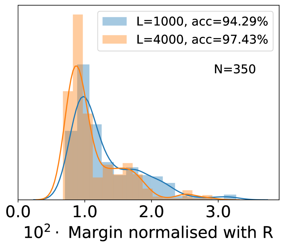
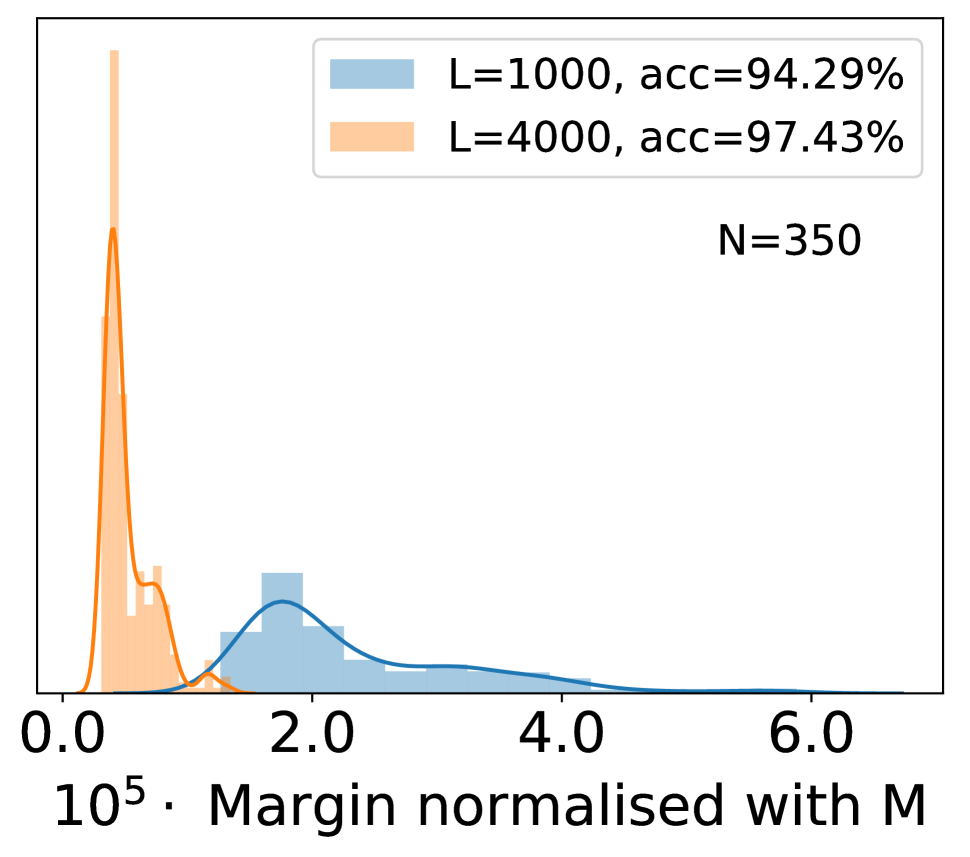
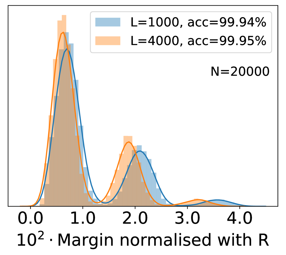
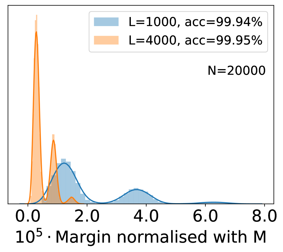
Figure 2: Distribution of normalised margins for different values of $N$ and $L$

References

- Allen-Zhu, Li, and Liang (2019) Allen-Zhu, Z.; Li, Y.; and Liang, Y. 2019. Learning and Generalization in Overparameterized Neural Networks, Going Beyond Two Layers. In Wallach, H.; Larochelle, H.; Beygelzimer, A.; d Alché-Buc, F.; Fox, E.; and Garnett, R., eds., Advances in Neural Information Processing Systems 32, 6155–6166. Curran Associates, Inc.
- Anthony and Bartlett (2002) Anthony, M.; and Bartlett, P. 2002. Neural Network Learning: Theoretical Foundations. ISBN 978-0-521-57353-5. doi:10.1017/CBO9780511624216.
- Arora et al. (2019) Arora, S.; Du, S. S.; Hu, W.; Li, Z.; and Wang, R. 2019. Fine-Grained Analysis of Optimization and Generalization for Overparameterized Two-Layer Neural Networks. arXiv e-prints arXiv:1901.08584.
- Arora et al. (2018) Arora, S.; Ge, R.; Neyshabur, B.; and Zhang, Y. 2018. Stronger Generalization Bounds for Deep Nets via a Compression Approach. In Dy, J.; and Krause, A., eds., Proceedings of the 35th International Conference on Machine Learning, volume 80 of Proceedings of Machine Learning Research, 254–263. Stockholm, Sweden: PMLR.
- Asadi, Abbe, and Verdu (2018) Asadi, A.; Abbe, E.; and Verdu, S. 2018. Chaining Mutual Information and Tightening Generalization Bounds. In Bengio, S.; Wallach, H.; Larochelle, H.; Grauman, K.; Cesa-Bianchi, N.; and Garnett, R., eds., Advances in Neural Information Processing Systems 31, 7234–7243. Curran Associates, Inc.
- Bartlett and Shawe-taylor (1998) Bartlett, P.; and Shawe-taylor, J. 1998. Generalization Performance of Support Vector Machines and Other Pattern Classifiers.
- Bartlett (1997) Bartlett, P. L. 1997. For Valid Generalization the Size of the Weights is More Important than the Size of the Network. In Mozer, M. C.; Jordan, M. I.; and Petsche, T., eds., Advances in Neural Information Processing Systems 9, 134–140. MIT Press.
- Bartlett (1998) Bartlett, P. L. 1998. The sample complexity of pattern classification with neural networks: the size of the weights is more important than the size of the network. IEEE Transactions on Information Theory 44(2): 525–536. doi:10.1109/18.661502.
- Bartlett, Foster, and Telgarsky (2017) Bartlett, P. L.; Foster, D. J.; and Telgarsky, M. J. 2017. Spectrally-normalized margin bounds for neural networks. 6240–6249. Curran Associates, Inc.
- Bartlett and Mendelson (2002) Bartlett, P. L.; and Mendelson, S. 2002. Rademacher and Gaussian complexities: Risk bounds and structural results. Journal of Machine Learning Research 3(Nov): 463–482.
- Brutzkus et al. (2018) Brutzkus, A.; Globerson, A.; Malach, E.; and Shalev-Shwartz, S. 2018. SGD Learns Over-parameterized Networks that Provably Generalize on Linearly Separable Data. In International Conference on Learning Representations.
- Cao and Gu (2019) Cao, Y.; and Gu, Q. 2019. Generalization Bounds of Stochastic Gradient Descent for Wide and Deep Neural Networks. arXiv e-prints arXiv:1905.13210.
- Chen, Li, and Zhao (2019) Chen, M.; Li, X.; and Zhao, T. 2019. On Generalization Bounds of a Family of Recurrent Neural Networks.
- Du et al. (2018) Du, S. S.; Wang, Y.; Zhai, X.; Balakrishnan, S.; Salakhutdinov, R. R.; and Singh, A. 2018. How Many Samples are Needed to Estimate a Convolutional Neural Network? In Bengio, S.; Wallach, H.; Larochelle, H.; Grauman, K.; Cesa-Bianchi, N.; and Garnett, R., eds., Advances in Neural Information Processing Systems 31, 373–383. Curran Associates, Inc.
- Du et al. (2019) Du, S. S.; Zhai, X.; Poczos, B.; and Singh, A. 2019. Gradient Descent Provably Optimizes Over-parameterized Neural Networks. In International Conference on Learning Representations.
- Dziugaite and Roy (2018) Dziugaite, G.; and Roy, D. 2018. Data-dependent PAC-Bayes priors via differential privacy .
- Fazlyab et al. (2019) Fazlyab, M.; Robey, A.; Hassani, H.; Morari, M.; and Pappas, G. J. 2019. Efficient and Accurate Estimation of Lipschitz Constants for Deep Neural Networks. CoRR abs/1906.04893.
- Frankle and Carbin (2019) Frankle, J.; and Carbin, M. 2019. The Lottery Ticket Hypothesis: Finding Sparse, Trainable Neural Networks. In International Conference on Learning Representations.
- Giné and Guillou (2001) Giné, E.; and Guillou, A. 2001. On consistency of kernel density estimators for randomly censored data: Rates holding uniformly over adaptive intervals. Annales de l’Institut Henri Poincare (B) Probability and Statistics 37: 503–522. doi:10.1016/S0246-0203(01)01081-0.
- Golowich, Rakhlin, and Shamir (2018) Golowich, N.; Rakhlin, A.; and Shamir, O. 2018. Size-Independent Sample Complexity of Neural Networks. In Bubeck, S.; Perchet, V.; and Rigollet, P., eds., Proceedings of the 31st Conference On Learning Theory, volume 75 of Proceedings of Machine Learning Research, 297–299. PMLR.
- Goodfellow, Shlens, and Szegedy (2015) Goodfellow, I.; Shlens, J.; and Szegedy, C. 2015. Explaining and Harnessing Adversarial Examples. In International Conference on Learning Representations.
- Guermeur (2002) Guermeur, Y. 2002. Combining Discriminant Models with New Multi-Class SVMs. Pattern Analysis & Applications 5(2): 168–179. ISSN 1433-7541. doi:10.1007/s100440200015.
- Guermeur (2007) Guermeur, Y. 2007. VC Theory of Large Margin Multi-Category Classifiers. Journal of Machine Learning Research 8: 2551–2594.
- Guermeur (2017) Guermeur, Y. 2017. Lp-norm Sauer–Shelah lemma for margin multi-category classifiers. Journal of Computer and System Sciences 89: 450 – 473. ISSN 0022-0000. doi:https://doi.org/10.1016/j.jcss.2017.06.003.
- Harvey, Liaw, and Mehrabian (2017) Harvey, N.; Liaw, C.; and Mehrabian, A. 2017. Nearly-tight VC-dimension bounds for piecewise linear neural networks. In Kale, S.; and Shamir, O., eds., Proceedings of the 2017 Conference on Learning Theory, volume 65 of Proceedings of Machine Learning Research, 1064–1068. Amsterdam, Netherlands: PMLR.
- He, Liu, and Tao (2019) He, F.; Liu, T.; and Tao, D. 2019. Why ResNet Works? Residuals Generalize. arXiv e-prints arXiv:1904.01367.
- He et al. (2016) He, K.; Zhang, X.; Ren, S.; and Sun, J. 2016. Deep Residual Learning for Image Recognition. In CVPR, 770–778. IEEE Computer Society.
- Jacot, Gabriel, and Hongler (2018) Jacot, A.; Gabriel, F.; and Hongler, C. 2018. Neural Tangent Kernel: Convergence and Generalization in Neural Networks. CoRR abs/1806.07572.
- Karras, Laine, and Aila (2018) Karras, T.; Laine, S.; and Aila, T. 2018. A Style-Based Generator Architecture for Generative Adversarial Networks. CoRR abs/1812.04948.
- Koltchinskii and Panchenko (2002) Koltchinskii, V.; and Panchenko, D. 2002. Empirical Margin Distributions and Bounding the Generalization Error of Combined Classifiers. Ann. Statist. 30(1): 1–50. doi:10.1214/aos/1015362183.
- Krizhevsky, Sutskever, and Hinton (2012) Krizhevsky, A.; Sutskever, I.; and Hinton, G. E. 2012. ImageNet Classification with Deep Convolutional Neural Networks. In Pereira, F.; Burges, C. J. C.; Bottou, L.; and Weinberger, K. Q., eds., Advances in Neural Information Processing Systems 25, 1097–1105. Curran Associates, Inc.
- Latorre, Rolland, and Cevher (2020) Latorre, F.; Rolland, P.; and Cevher, V. 2020. Lipschitz constant estimation of Neural Networks via sparse polynomial optimization. In International Conference on Learning Representations. URL https://openreview.net/forum?id=rJe4_xSFDB.
- Lauer (2018) Lauer, F. 2018. Error bounds with almost radical dependence on the number of components for multi-category classification, vector quantization and switching regression. In Conférence sur l’Apprentissage automatique (CAp) - French Conference on Machine Learning (FCML), Proc. of the French Conference on Machine Learning (CAp/FCML). Rouen, France.
- Lee and Raginsky (2019) Lee, J.; and Raginsky, M. 2019. Learning Finite-Dimensional Coding Schemes with Nonlinear Reconstruction Maps. SIAM Journal on Mathematics of Data Science 1: 617–642. doi:10.1137/18M1234461.
- Lei et al. (2019) Lei, Y.; Dogan, Ü.; Zhou, D.; and Kloft, M. 2019. Data-Dependent Generalization Bounds for Multi-Class Classification. IEEE Trans. Information Theory 65(5): 2995–3021. doi:10.1109/TIT.2019.2893916.
- Li et al. (2019) Li, X.; Lu, J.; Wang, Z.; Haupt, J.; and Zhao, T. 2019. On Tighter Generalization Bounds for Deep Neural Networks: CNNs, ResNets, and Beyond.
- Lin and Zhang (2019) Lin, S.; and Zhang, J. 2019. Generalization Bounds for Convolutional Neural Networks.
- Long and Sedghi (2020) Long, P. M.; and Sedghi, H. 2020. Size-free generalization bounds for convolutional neural networks. In International Conference on Learning Representations.
- Mohri, Rostamizadeh, and Talwalkar (2018) Mohri, M.; Rostamizadeh, A.; and Talwalkar, A. 2018. Foundations of Machine Learning. Adaptive Computation and Machine Learning. Cambridge, MA: MIT Press, 2 edition. ISBN 978-0-262-03940-6.
- Musayeva, Lauer, and Guermeur (2019) Musayeva, K.; Lauer, F.; and Guermeur, Y. 2019. Rademacher complexity and generalization performance of multi-category margin classifiers. Neurocomputing 342: 6 – 15. ISSN 0925-2312. doi:https://doi.org/10.1016/j.neucom.2018.11.096. Advances in artificial neural networks, machine learning and computational intelligence.
- Nagarajan and Kolter (2019) Nagarajan, V.; and Kolter, J. Z. 2019. Deterministic PAC-Bayesian generalization bounds for deep networks via generalizing noise-resilience. CoRR abs/1905.13344.
- Neyshabur, Bhojanapalli, and Srebro (2018) Neyshabur, B.; Bhojanapalli, S.; and Srebro, N. 2018. A PAC-Bayesian Approach to Spectrally-Normalized Margin Bounds for Neural Networks. In International Conference on Learning Representations. openreview.net.
- Neyshabur et al. (2019, to appear) Neyshabur, B.; Li, Z.; Bhojanapalli, S.; LeCun, Y.; and Srebro, N. 2019, to appear. The role of over-parametrization in generalization of neural networks. In International Conference on Learning Representations.
- Neyshabur, Tomioka, and Srebro (2015) Neyshabur, B.; Tomioka, R.; and Srebro, N. 2015. Norm-Based Capacity Control in Neural Networks. In GrÃŒnwald, P.; Hazan, E.; and Kale, S., eds., Proceedings of The 28th Conference on Learning Theory, volume 40 of Proceedings of Machine Learning Research, 1376–1401. Paris, France: PMLR.
- Pisier (1980-1981) Pisier, G. 1980-1981. Remarques sur un résultat non publié de B. Maurey. Séminaire Analyse fonctionnelle (dit "Maurey-Schwartz") Talk:5.
- Platen (1986) Platen, E. 1986. Pollard, D.:Convergence of stochastic processes. (Springer series in statistics). Springer-Verlag, New York - Berlin - Heidelberg - Tokyo 1984, 216 pp., 36 illustr., DM 82. Biometrical Journal 28(5): 644–644. doi:10.1002/bimj.4710280516.
- Prabhu and Varma (2014) Prabhu, Y.; and Varma, M. 2014. FastXML: A Fast, Accurate and Stable Tree-classifier for Extreme Multi-label Learning. In Proceedings of the 20th ACM SIGKDD International Conference on Knowledge Discovery and Data Mining, KDD ’14, 263–272. New York, NY, USA: ACM. ISBN 978-1-4503-2956-9. doi:10.1145/2623330.2623651.
- Scott (2014) Scott, C. 2014. Rademacher Complexity. Lecture Notes Statistical Learning Theory.
- Sedghi, Gupta, and Long (2019) Sedghi, H.; Gupta, V.; and Long, P. M. 2019. The Singular Values of Convolutional Layers. In International Conference on Learning Representations.
- Silver et al. (2018) Silver, D.; Hubert, T.; Schrittwieser, J.; Antonoglou, I.; Lai, M.; Guez, A.; Lanctot, M.; Sifre, L.; Kumaran, D.; Graepel, T.; Lillicrap, T.; Simonyan, K.; and Hassabis, D. 2018. A general reinforcement learning algorithm that masters chess, shogi, and Go through self-play. Science 362(6419): 1140–1144. ISSN 0036-8075. doi:10.1126/science.aar6404.
- Suzuki (2018) Suzuki, T. 2018. Fast generalization error bound of deep learning from a kernel perspective. In Storkey, A.; and Perez-Cruz, F., eds., Proceedings of the Twenty-First International Conference on Artificial Intelligence and Statistics, volume 84 of Proceedings of Machine Learning Research, 1397–1406. Playa Blanca, Lanzarote, Canary Islands: PMLR.
- Talagrand (1994) Talagrand, M. 1994. Sharper Bounds for Gaussian and Empirical Processes. The Annals of Probability 22(1): 28–76. ISSN 00911798.
- Talagrand (1996) Talagrand, M. 1996. New concentration inequalities in product spaces. Inventiones mathematicae 126(3): 505–563. ISSN 1432-1297. doi:10.1007/s002220050108.
- Wei and Ma (2019) Wei, C.; and Ma, T. 2019. Data-dependent Sample Complexity of Deep Neural Networks via Lipschitz Augmentation. In Wallach, H.; Larochelle, H.; Beygelzimer, A.; d'Alché-Buc, F.; Fox, E.; and Garnett, R., eds., Advances in Neural Information Processing Systems 32, 9725–9736. Curran Associates, Inc.
- Zhang et al. (2017) Zhang, C.; Bengio, S.; Hardt, M.; Recht, B.; and Vinyals, O. 2017. Understanding deep learning requires rethinking generalization.
- Zhang, Lei, and Dhillon (2018) Zhang, J.; Lei, Q.; and Dhillon, I. S. 2018. Stabilizing Gradients for Deep Neural Networks via Efficient SVD Parameterization. In ICML, volume 80 of Proceedings of Machine Learning Research, 5801–5809. PMLR.
- Zhang (2002) Zhang, T. 2002. Covering Number Bounds of Certain Regularized Linear Function Classes. J. Mach. Learn. Res. 2: 527–550. ISSN 1532-4435. doi:10.1162/153244302760200713.
- Zhou et al. (2019) Zhou, W.; Veitch, V.; Austern, M.; Adams, R. P.; and Orbanz, P. 2019. Non-vacuous Generalization Bounds at the ImageNet Scale: a PAC-Bayesian Compression Approach. In International Conference on Learning Representations. openreview.net.
- Zou et al. (2018) Zou, D.; Cao, Y.; Zhou, D.; and Gu, Q. 2018. Stochastic Gradient Descent Optimizes Over-parameterized Deep ReLU Networks. CoRR abs/1811.08888.

References

- Allen-Zhu, Li, and Liang (2019) Allen-Zhu, Z.; Li, Y.; and Liang, Y. 2019. Learning and Generalization in Overparameterized Neural Networks, Going Beyond Two Layers. In Wallach, H.; Larochelle, H.; Beygelzimer, A.; d Alché-Buc, F.; Fox, E.; and Garnett, R., eds., Advances in Neural Information Processing Systems 32, 6155–6166. Curran Associates, Inc.
- Anthony and Bartlett (2002) Anthony, M.; and Bartlett, P. 2002. Neural Network Learning: Theoretical Foundations. ISBN 978-0-521-57353-5. doi:10.1017/CBO9780511624216.
- Arora et al. (2019) Arora, S.; Du, S. S.; Hu, W.; Li, Z.; and Wang, R. 2019. Fine-Grained Analysis of Optimization and Generalization for Overparameterized Two-Layer Neural Networks. arXiv e-prints arXiv:1901.08584.
- Arora et al. (2018) Arora, S.; Ge, R.; Neyshabur, B.; and Zhang, Y. 2018. Stronger Generalization Bounds for Deep Nets via a Compression Approach. In Dy, J.; and Krause, A., eds., Proceedings of the 35th International Conference on Machine Learning, volume 80 of Proceedings of Machine Learning Research, 254–263. Stockholm, Sweden: PMLR.
- Asadi, Abbe, and Verdu (2018) Asadi, A.; Abbe, E.; and Verdu, S. 2018. Chaining Mutual Information and Tightening Generalization Bounds. In Bengio, S.; Wallach, H.; Larochelle, H.; Grauman, K.; Cesa-Bianchi, N.; and Garnett, R., eds., Advances in Neural Information Processing Systems 31, 7234–7243. Curran Associates, Inc.
- Bartlett and Shawe-taylor (1998) Bartlett, P.; and Shawe-taylor, J. 1998. Generalization Performance of Support Vector Machines and Other Pattern Classifiers.
- Bartlett (1997) Bartlett, P. L. 1997. For Valid Generalization the Size of the Weights is More Important than the Size of the Network. In Mozer, M. C.; Jordan, M. I.; and Petsche, T., eds., Advances in Neural Information Processing Systems 9, 134–140. MIT Press.
- Bartlett (1998) Bartlett, P. L. 1998. The sample complexity of pattern classification with neural networks: the size of the weights is more important than the size of the network. IEEE Transactions on Information Theory 44(2): 525–536. doi:10.1109/18.661502.
- Bartlett, Foster, and Telgarsky (2017) Bartlett, P. L.; Foster, D. J.; and Telgarsky, M. J. 2017. Spectrally-normalized margin bounds for neural networks. 6240–6249. Curran Associates, Inc.
- Bartlett and Mendelson (2002) Bartlett, P. L.; and Mendelson, S. 2002. Rademacher and Gaussian complexities: Risk bounds and structural results. Journal of Machine Learning Research 3(Nov): 463–482.
- Brutzkus et al. (2018) Brutzkus, A.; Globerson, A.; Malach, E.; and Shalev-Shwartz, S. 2018. SGD Learns Over-parameterized Networks that Provably Generalize on Linearly Separable Data. In International Conference on Learning Representations.
- Cao and Gu (2019) Cao, Y.; and Gu, Q. 2019. Generalization Bounds of Stochastic Gradient Descent for Wide and Deep Neural Networks. arXiv e-prints arXiv:1905.13210.
- Chen, Li, and Zhao (2019) Chen, M.; Li, X.; and Zhao, T. 2019. On Generalization Bounds of a Family of Recurrent Neural Networks.
- Du et al. (2018) Du, S. S.; Wang, Y.; Zhai, X.; Balakrishnan, S.; Salakhutdinov, R. R.; and Singh, A. 2018. How Many Samples are Needed to Estimate a Convolutional Neural Network? In Bengio, S.; Wallach, H.; Larochelle, H.; Grauman, K.; Cesa-Bianchi, N.; and Garnett, R., eds., Advances in Neural Information Processing Systems 31, 373–383. Curran Associates, Inc.
- Du et al. (2019) Du, S. S.; Zhai, X.; Poczos, B.; and Singh, A. 2019. Gradient Descent Provably Optimizes Over-parameterized Neural Networks. In International Conference on Learning Representations.
- Dziugaite and Roy (2018) Dziugaite, G.; and Roy, D. 2018. Data-dependent PAC-Bayes priors via differential privacy .
- Fazlyab et al. (2019) Fazlyab, M.; Robey, A.; Hassani, H.; Morari, M.; and Pappas, G. J. 2019. Efficient and Accurate Estimation of Lipschitz Constants for Deep Neural Networks. CoRR abs/1906.04893.
- Frankle and Carbin (2019) Frankle, J.; and Carbin, M. 2019. The Lottery Ticket Hypothesis: Finding Sparse, Trainable Neural Networks. In International Conference on Learning Representations.
- Giné and Guillou (2001) Giné, E.; and Guillou, A. 2001. On consistency of kernel density estimators for randomly censored data: Rates holding uniformly over adaptive intervals. Annales de l’Institut Henri Poincare (B) Probability and Statistics 37: 503–522. doi:10.1016/S0246-0203(01)01081-0.
- Golowich, Rakhlin, and Shamir (2018) Golowich, N.; Rakhlin, A.; and Shamir, O. 2018. Size-Independent Sample Complexity of Neural Networks. In Bubeck, S.; Perchet, V.; and Rigollet, P., eds., Proceedings of the 31st Conference On Learning Theory, volume 75 of Proceedings of Machine Learning Research, 297–299. PMLR.
- Goodfellow, Shlens, and Szegedy (2015) Goodfellow, I.; Shlens, J.; and Szegedy, C. 2015. Explaining and Harnessing Adversarial Examples. In International Conference on Learning Representations.
- Guermeur (2002) Guermeur, Y. 2002. Combining Discriminant Models with New Multi-Class SVMs. Pattern Analysis & Applications 5(2): 168–179. ISSN 1433-7541. doi:10.1007/s100440200015.
- Guermeur (2007) Guermeur, Y. 2007. VC Theory of Large Margin Multi-Category Classifiers. Journal of Machine Learning Research 8: 2551–2594.
- Guermeur (2017) Guermeur, Y. 2017. Lp-norm Sauer–Shelah lemma for margin multi-category classifiers. Journal of Computer and System Sciences 89: 450 – 473. ISSN 0022-0000. doi:https://doi.org/10.1016/j.jcss.2017.06.003.
- Harvey, Liaw, and Mehrabian (2017) Harvey, N.; Liaw, C.; and Mehrabian, A. 2017. Nearly-tight VC-dimension bounds for piecewise linear neural networks. In Kale, S.; and Shamir, O., eds., Proceedings of the 2017 Conference on Learning Theory, volume 65 of Proceedings of Machine Learning Research, 1064–1068. Amsterdam, Netherlands: PMLR.
- He, Liu, and Tao (2019) He, F.; Liu, T.; and Tao, D. 2019. Why ResNet Works? Residuals Generalize. arXiv e-prints arXiv:1904.01367.
- He et al. (2016) He, K.; Zhang, X.; Ren, S.; and Sun, J. 2016. Deep Residual Learning for Image Recognition. In CVPR, 770–778. IEEE Computer Society.
- Jacot, Gabriel, and Hongler (2018) Jacot, A.; Gabriel, F.; and Hongler, C. 2018. Neural Tangent Kernel: Convergence and Generalization in Neural Networks. CoRR abs/1806.07572.
- Karras, Laine, and Aila (2018) Karras, T.; Laine, S.; and Aila, T. 2018. A Style-Based Generator Architecture for Generative Adversarial Networks. CoRR abs/1812.04948.
- Koltchinskii and Panchenko (2002) Koltchinskii, V.; and Panchenko, D. 2002. Empirical Margin Distributions and Bounding the Generalization Error of Combined Classifiers. Ann. Statist. 30(1): 1–50. doi:10.1214/aos/1015362183.
- Krizhevsky, Sutskever, and Hinton (2012) Krizhevsky, A.; Sutskever, I.; and Hinton, G. E. 2012. ImageNet Classification with Deep Convolutional Neural Networks. In Pereira, F.; Burges, C. J. C.; Bottou, L.; and Weinberger, K. Q., eds., Advances in Neural Information Processing Systems 25, 1097–1105. Curran Associates, Inc.
- Latorre, Rolland, and Cevher (2020) Latorre, F.; Rolland, P.; and Cevher, V. 2020. Lipschitz constant estimation of Neural Networks via sparse polynomial optimization. In International Conference on Learning Representations. URL https://openreview.net/forum?id=rJe4_xSFDB.
- Lauer (2018) Lauer, F. 2018. Error bounds with almost radical dependence on the number of components for multi-category classification, vector quantization and switching regression. In Conférence sur l’Apprentissage automatique (CAp) - French Conference on Machine Learning (FCML), Proc. of the French Conference on Machine Learning (CAp/FCML). Rouen, France.
- Lee and Raginsky (2019) Lee, J.; and Raginsky, M. 2019. Learning Finite-Dimensional Coding Schemes with Nonlinear Reconstruction Maps. SIAM Journal on Mathematics of Data Science 1: 617–642. doi:10.1137/18M1234461.
- Lei et al. (2019) Lei, Y.; Dogan, Ü.; Zhou, D.; and Kloft, M. 2019. Data-Dependent Generalization Bounds for Multi-Class Classification. IEEE Trans. Information Theory 65(5): 2995–3021. doi:10.1109/TIT.2019.2893916.
- Li et al. (2019) Li, X.; Lu, J.; Wang, Z.; Haupt, J.; and Zhao, T. 2019. On Tighter Generalization Bounds for Deep Neural Networks: CNNs, ResNets, and Beyond.
- Lin and Zhang (2019) Lin, S.; and Zhang, J. 2019. Generalization Bounds for Convolutional Neural Networks.
- Long and Sedghi (2020) Long, P. M.; and Sedghi, H. 2020. Size-free generalization bounds for convolutional neural networks. In International Conference on Learning Representations.
- Mohri, Rostamizadeh, and Talwalkar (2018) Mohri, M.; Rostamizadeh, A.; and Talwalkar, A. 2018. Foundations of Machine Learning. Adaptive Computation and Machine Learning. Cambridge, MA: MIT Press, 2 edition. ISBN 978-0-262-03940-6.
- Musayeva, Lauer, and Guermeur (2019) Musayeva, K.; Lauer, F.; and Guermeur, Y. 2019. Rademacher complexity and generalization performance of multi-category margin classifiers. Neurocomputing 342: 6 – 15. ISSN 0925-2312. doi:https://doi.org/10.1016/j.neucom.2018.11.096. Advances in artificial neural networks, machine learning and computational intelligence.
- Nagarajan and Kolter (2019) Nagarajan, V.; and Kolter, J. Z. 2019. Deterministic PAC-Bayesian generalization bounds for deep networks via generalizing noise-resilience. CoRR abs/1905.13344.
- Neyshabur, Bhojanapalli, and Srebro (2018) Neyshabur, B.; Bhojanapalli, S.; and Srebro, N. 2018. A PAC-Bayesian Approach to Spectrally-Normalized Margin Bounds for Neural Networks. In International Conference on Learning Representations. openreview.net.
- Neyshabur et al. (2019, to appear) Neyshabur, B.; Li, Z.; Bhojanapalli, S.; LeCun, Y.; and Srebro, N. 2019, to appear. The role of over-parametrization in generalization of neural networks. In International Conference on Learning Representations.
- Neyshabur, Tomioka, and Srebro (2015) Neyshabur, B.; Tomioka, R.; and Srebro, N. 2015. Norm-Based Capacity Control in Neural Networks. In GrÃŒnwald, P.; Hazan, E.; and Kale, S., eds., Proceedings of The 28th Conference on Learning Theory, volume 40 of Proceedings of Machine Learning Research, 1376–1401. Paris, France: PMLR.
- Pisier (1980-1981) Pisier, G. 1980-1981. Remarques sur un résultat non publié de B. Maurey. Séminaire Analyse fonctionnelle (dit "Maurey-Schwartz") Talk:5.
- Platen (1986) Platen, E. 1986. Pollard, D.:Convergence of stochastic processes. (Springer series in statistics). Springer-Verlag, New York - Berlin - Heidelberg - Tokyo 1984, 216 pp., 36 illustr., DM 82. Biometrical Journal 28(5): 644–644. doi:10.1002/bimj.4710280516.
- Prabhu and Varma (2014) Prabhu, Y.; and Varma, M. 2014. FastXML: A Fast, Accurate and Stable Tree-classifier for Extreme Multi-label Learning. In Proceedings of the 20th ACM SIGKDD International Conference on Knowledge Discovery and Data Mining, KDD ’14, 263–272. New York, NY, USA: ACM. ISBN 978-1-4503-2956-9. doi:10.1145/2623330.2623651.
- Scott (2014) Scott, C. 2014. Rademacher Complexity. Lecture Notes Statistical Learning Theory.
- Sedghi, Gupta, and Long (2019) Sedghi, H.; Gupta, V.; and Long, P. M. 2019. The Singular Values of Convolutional Layers. In International Conference on Learning Representations.
- Silver et al. (2018) Silver, D.; Hubert, T.; Schrittwieser, J.; Antonoglou, I.; Lai, M.; Guez, A.; Lanctot, M.; Sifre, L.; Kumaran, D.; Graepel, T.; Lillicrap, T.; Simonyan, K.; and Hassabis, D. 2018. A general reinforcement learning algorithm that masters chess, shogi, and Go through self-play. Science 362(6419): 1140–1144. ISSN 0036-8075. doi:10.1126/science.aar6404.
- Suzuki (2018) Suzuki, T. 2018. Fast generalization error bound of deep learning from a kernel perspective. In Storkey, A.; and Perez-Cruz, F., eds., Proceedings of the Twenty-First International Conference on Artificial Intelligence and Statistics, volume 84 of Proceedings of Machine Learning Research, 1397–1406. Playa Blanca, Lanzarote, Canary Islands: PMLR.
- Talagrand (1994) Talagrand, M. 1994. Sharper Bounds for Gaussian and Empirical Processes. The Annals of Probability 22(1): 28–76. ISSN 00911798.
- Talagrand (1996) Talagrand, M. 1996. New concentration inequalities in product spaces. Inventiones mathematicae 126(3): 505–563. ISSN 1432-1297. doi:10.1007/s002220050108.
- Wei and Ma (2019) Wei, C.; and Ma, T. 2019. Data-dependent Sample Complexity of Deep Neural Networks via Lipschitz Augmentation. In Wallach, H.; Larochelle, H.; Beygelzimer, A.; d'Alché-Buc, F.; Fox, E.; and Garnett, R., eds., Advances in Neural Information Processing Systems 32, 9725–9736. Curran Associates, Inc.
- Zhang et al. (2017) Zhang, C.; Bengio, S.; Hardt, M.; Recht, B.; and Vinyals, O. 2017. Understanding deep learning requires rethinking generalization.
- Zhang, Lei, and Dhillon (2018) Zhang, J.; Lei, Q.; and Dhillon, I. S. 2018. Stabilizing Gradients for Deep Neural Networks via Efficient SVD Parameterization. In ICML, volume 80 of Proceedings of Machine Learning Research, 5801–5809. PMLR.
- Zhang (2002) Zhang, T. 2002. Covering Number Bounds of Certain Regularized Linear Function Classes. J. Mach. Learn. Res. 2: 527–550. ISSN 1532-4435. doi:10.1162/153244302760200713.
- Zhou et al. (2019) Zhou, W.; Veitch, V.; Austern, M.; Adams, R. P.; and Orbanz, P. 2019. Non-vacuous Generalization Bounds at the ImageNet Scale: a PAC-Bayesian Compression Approach. In International Conference on Learning Representations. openreview.net.
- Zou et al. (2018) Zou, D.; Cao, Y.; Zhou, D.; and Gu, Q. 2018. Stochastic Gradient Descent Optimizes Over-parameterized Deep ReLU Networks. CoRR abs/1811.08888.