Cascading Non-Stationary Bandits: Online Learning to Rank in the Non-Stationary Cascade Model

Chang Li &Maarten de Rijke University of Amsterdam {c.li, derijke}@uva.nl
Abstract

Non-stationarity appears in many online applications such as web search and advertising. In this paper, we study the online learning to rank problem in a non-stationary environment where user preferences change abruptly at an unknown moment in time. We consider the problem of identifying the K𝐾K most attractive items and propose cascading non-stationary bandits, an online learning variant of the cascading model, where a user browses a ranked list from top to bottom and clicks on the first attractive item. We propose two algorithms for solving this non-stationary problem: π–’π–Ίπ—Œπ–Όπ–Ίπ–½π–Ύπ–£π–΄π–’π–‘π–’π–Ίπ—Œπ–Όπ–Ίπ–½π–Ύπ–£π–΄π–’π–‘{\sf CascadeDUCB} and π–’π–Ίπ—Œπ–Όπ–Ίπ–½π–Ύπ–²π–Άπ–΄π–’π–‘π–’π–Ίπ—Œπ–Όπ–Ίπ–½π–Ύπ–²π–Άπ–΄π–’π–‘{\sf CascadeSWUCB}. We analyze their performance and derive gap-dependent upper bounds on the n𝑛n-step regret of these algorithms. We also establish a lower bound on the regret for cascading non-stationary bandits and show that both algorithms match the lower bound up to a logarithmic factor. Finally, we evaluate their performance on a real-world web search click dataset.

1 Introduction

Learning to rank LTRΒ Liu (2009) is a combination of machine learning and information retrieval. It is a core problem in many applications, such as web search and recommendationΒ Liu (2009); Zoghi et al. (2017). The goal of learning to rank (LTR) is to rank items, e.g., documents, and show the top K𝐾K items to a user. Traditional LTR algorithms are supervised, offline algorithms; they learn rankers from human annotated dataΒ Qin et al. (2010) and/or users’ historical interactionsΒ Joachims (2002). Every day billions of users interact with modern search engines and leave a trail of interactions. It is feasible and important to design online algorithms that directly learn from such user clicks to help improve users’ online experience. Indeed, recent studies show that even well-trained production rankers can be optimized by using users’ online interactions, such as clicksΒ Zoghi et al. (2016).

Generally, interaction data is noisyΒ Joachims (2002), which gives rise to the well-known exploration vs.Β exploitation dilemma. Multi-armed banditΒ (MAB)Β Auer et al. (2002) algorithms have been designed to balance exploration and exploitation. Based on multi-armed bandits, many online LTR algorithms have been publishedΒ Radlinski et al. (2008); Kveton et al. (2015); Katariya et al. (2016); LagrΓ©e et al. (2016); Zoghi et al. (2017); Li et al. (2019). These algorithms address the exploration vs. exploitation dilemma in an elegant way and aim to maximize user satisfaction in a stationary environment where users do not change their preferences over time. Moreover, they often come with regret bounds.

Despite the success of the algorithms mentioned above in the stationary case, they may have linear regret in a non-stationary environment where users may change their preferences abruptly at any unknown moment in time. Non-stationarity widely exists in real-world application domains, such as search engines and recommender systemsΒ Yu and Mannor (2009); Pereira et al. (2018); Wu et al. (2018); Jagerman et al. (2019). Particularly, we consider abruptly changing environments where user preferences remain constant in certain time periods, named epochs, but change occurs abruptly at unknown moments called breakpoints. The abrupt changes in user preferences give rise to a new challenge of balancing β€œremembering” and β€œforgetting” Besbes et al. (2014): the more past observations an algorithm retains the higher the risk of making a biased estimator, while the fewer observations retained the higher stochastic error it has on the estimates of the user preferences.

In this paper, we propose cascading non-stationary bandits, an online variant of the cascade model (CM) Craswell et al. (2008) with the goal of identifying the K𝐾K most attractive items in a non-stationary environment. CM is a widely-used model of user click behavior Chuklin et al. (2015); Zoghi et al. (2017). In CM, a user browses the ranked list from top to bottom and clicks the first attractive item. The items ranked above the first clicked item are browsed but not attractive since they are not clicked. The items ranked below the first clicked item are not browsed since the user stops browsing the ranked list after a click. Although CM is a simple model, it effectively explains user behavior Kveton et al. (2015).

Our key technical contributions in this paper are: (1) We formalize a non-stationary online learning to rank (OLTR) problem as cascading non-stationary bandits. (2) We propose two algorithms, π–’π–Ίπ—Œπ–Όπ–Ίπ–½π–Ύπ–£π–΄π–’π–‘π–’π–Ίπ—Œπ–Όπ–Ίπ–½π–Ύπ–£π–΄π–’π–‘{\sf CascadeDUCB} and π–’π–Ίπ—Œπ–Όπ–Ίπ–½π–Ύπ–²π–Άπ–΄π–’π–‘π–’π–Ίπ—Œπ–Όπ–Ίπ–½π–Ύπ–²π–Άπ–΄π–’π–‘{\sf CascadeSWUCB}, for solving it. They are motivated by discounted UCB (𝖣𝖴𝖒𝖑𝖣𝖴𝖒𝖑{\sf DUCB}) and sliding window UCB (𝖲𝖢𝖴𝖒𝖑𝖲𝖢𝖴𝖒𝖑{\sf SWUCB}), respectivelyΒ Garivier and Moulines (2011). π–’π–Ίπ—Œπ–Όπ–Ίπ–½π–Ύπ–£π–΄π–’π–‘π–’π–Ίπ—Œπ–Όπ–Ίπ–½π–Ύπ–£π–΄π–’π–‘{\sf CascadeDUCB} balances β€œremembering” and β€œforgetting” by using a discounting factor of past observations, and π–’π–Ίπ—Œπ–Όπ–Ίπ–½π–Ύπ–²π–Άπ–΄π–’π–‘π–’π–Ίπ—Œπ–Όπ–Ίπ–½π–Ύπ–²π–Άπ–΄π–’π–‘{\sf CascadeSWUCB} balances the two by using statistics inside a fixed-size sliding window. (3) We derive gap-dependent upper bounds on the regret of the proposed algorithms. (4) We derive a lower bound on the regret of cascading non-stationary bandits. We show that the upper bounds match this lower bound up to a logarithmic factor. (5) We evaluate the performance of π–’π–Ίπ—Œπ–Όπ–Ίπ–½π–Ύπ–²π–Άπ–΄π–’π–‘π–’π–Ίπ—Œπ–Όπ–Ίπ–½π–Ύπ–²π–Άπ–΄π–’π–‘{\sf CascadeSWUCB} and π–’π–Ίπ—Œπ–Όπ–Ίπ–½π–Ύπ–£π–΄π–’π–‘π–’π–Ίπ—Œπ–Όπ–Ίπ–½π–Ύπ–£π–΄π–’π–‘{\sf CascadeDUCB} empirically on a real-world web search click dataset.

2 Background

We define the learning problem at the core of this paper in terms of cascading non-stationary bandits. Their definition builds on the CM and its online variant cascading bandits, which we review in this section.

We write [n]delimited-[]𝑛[n] for {1,…,n}1…𝑛\left\{1,\dots,n\right\}. For sets A𝐴A and B𝐡B, we write ABsuperscript𝐴𝐡A^{B} for the set of all vectors whose entries are indexed by B𝐡B and take values from A𝐴A. We use boldface letters to denote random variables. We denote a set of candidate items by π’Ÿ=[L]π’Ÿdelimited-[]𝐿\mathcal{D}=[L], e.g., a set of preselected documents. The presented ranked list is denoted as β„›βˆˆΞ K​(π’Ÿ)β„›subscriptΞ πΎπ’Ÿ\mathcal{R}\in\Pi_{K}(\mathcal{D}), where Ξ K​(π’Ÿ)subscriptΞ πΎπ’Ÿ\Pi_{K}(\mathcal{D}) denotes the set of all possible combinations of K𝐾K distinct items from π’Ÿπ’Ÿ\mathcal{D}. The item at position kπ‘˜k in β„›β„›\mathcal{R} is denoted as ℛ​(k)β„›π‘˜\mathcal{R}(k), and the position of item aπ‘Ža in β„›β„›\mathcal{R} is denoted as β„›βˆ’1​(a)superscriptβ„›1π‘Ž\mathcal{R}^{-1}(a)

2.1 Cascade Model

We refer readers to Chuklin et al. (2015) for an introduction to click models. Briefly, a click model models a user’s interaction behavior with the search system. The user is presented with a K𝐾K-item ranked list β„›β„›\mathcal{R}. Then the user browses the list β„›β„›\mathcal{R} and clicks items that potentially attract him or her. Many click models have been proposed and each models a certain aspect of interaction behavior. We can parameterize a click model by attraction probabilities α∈[0,1]L𝛼superscript01𝐿\alpha\in[0,1]^{L} and a click model assumes:

Assumption 1.

The attraction probability α​(a)π›Όπ‘Ž\alpha(a) only depends on item aπ‘Ža and is independent of other items.

CM is a widely-used click modelΒ Craswell et al. (2008); Zoghi et al. (2017). In the CM, a user browses the ranked list β„›β„›\mathcal{R} from the first item ℛ​(1)β„›1\mathcal{R}(1) to the last item ℛ​(K)ℛ𝐾\mathcal{R}(K), which is called the cascading assumption. After the user browses an item ℛ​(i)ℛ𝑖\mathcal{R}(i), he or she clicks on ℛ​(i)ℛ𝑖\mathcal{R}(i) with attraction probability α​(ℛ​(i))𝛼ℛ𝑖\alpha(\mathcal{R}(i)), and then stops browsing the remaining items. Thus, the examination probability of item ℛ​(j)ℛ𝑗\mathcal{R}(j) equals the probability of no click on the higher ranked items: ∏i=1jβˆ’1(1βˆ’Ξ±β€‹(ℛ​(i)))superscriptsubscriptproduct𝑖1𝑗11𝛼ℛ𝑖\prod_{i=1}^{j-1}(1-\alpha(\mathcal{R}(i))). The expected number of clicks equals the probability of clicking any item in the list: 1βˆ’βˆi=1K(1βˆ’Ξ±β€‹(ℛ​(i)))1superscriptsubscriptproduct𝑖1𝐾1𝛼ℛ𝑖1-\prod_{i=1}^{K}(1-\alpha(\mathcal{R}(i))). Note that the reward does not depend on the order in β„›β„›\mathcal{R}, and thus, in the CM, the goal of ranking is to find the K𝐾K most attractive items.

The CM accepts at most one click in each search session. It cannot explain scenarios where a user may click multiple items. The CM has been extended in different ways to capture multi-click casesΒ Chapelle and Zhang (2009); Guo et al. (2009). Nevertheless, CM is still the fundamental click model and fits historical click data reasonably well. Thus, in this paper, we focus on the CM and in the next section we introduce an online variant of CM, called cascading bandits.

2.2 Cascading Bandits

Cascading bandits (CB) is defined by a tuple B=(π’Ÿ,P,K)π΅π’Ÿπ‘ƒπΎB=(\mathcal{D},P,K), where π’Ÿ=[L]π’Ÿdelimited-[]𝐿\mathcal{D}=[L] is the set of candidate items, K≀L𝐾𝐿K\leq L is the number of positions, P∈{0,1}L𝑃superscript01𝐿P\in\{0,1\}^{L} is a distribution over binary attractions.

In cascading bandits (CB), at time t𝑑t, a learning agent builds a ranked list 𝐑t∈ΠK​(π’Ÿ)subscript𝐑𝑑subscriptΞ πΎπ’Ÿ\mathbf{R}_{t}\in\Pi_{K}(\mathcal{D}) that depends on the historical observations up to t𝑑t and shows it to the user. 𝐀t∈{0,1}Lsubscript𝐀𝑑superscript01𝐿\mathbf{A}_{t}\in\{0,1\}^{L} is defined as the attraction indicator, which is drawn from P𝑃P and 𝐀t​(𝐑t​(i))subscript𝐀𝑑subscript𝐑𝑑𝑖\mathbf{A}_{t}(\mathbf{R}_{t}(i)) is the attraction indicator of item 𝐑t​(i)subscript𝐑𝑑𝑖\mathbf{R}_{t}(i). The user examines 𝐑tsubscript𝐑𝑑\mathbf{R}_{t} from 𝐑t​(1)subscript𝐑𝑑1\mathbf{R}_{t}(1) to 𝐑t​(K)subscript𝐑𝑑𝐾\mathbf{R}_{t}(K) and clicks the first attractive item. Since a CM allows at most one click each time, a random variable 𝐜tsubscriptπœπ‘‘\mathbf{c}_{t} is used to indicate the position of the clicked item, i.e., 𝐜t=arg​mini∈[K]β‘πŸ™β€‹{𝐀t​(𝐑t​(i))}subscriptπœπ‘‘subscriptargmin𝑖delimited-[]𝐾1subscript𝐀𝑑subscript𝐑𝑑𝑖\mathbf{c}_{t}=\operatorname{arg\,min}_{i\in[K]}\mathds{1}\{\mathbf{A}_{t}(\mathbf{R}_{t}(i))\}. If there is no attractive item, the user will not click, and we set 𝐜t=K+1subscriptπœπ‘‘πΎ1\mathbf{c}_{t}=K+1 to indicate this case. Specifically, if 𝐜t≀Ksubscriptπœπ‘‘πΎ\mathbf{c}_{t}\leq K, the user clicks an item, otherwise, the user does not click anything. After the click or browsing the last item in 𝐑tsubscript𝐑𝑑\mathbf{R}_{t}, the user leaves the search session. The click feedback 𝐜tsubscriptπœπ‘‘\mathbf{c}_{t} is then observed by the learning agent. Because of the cascading assumption, the agent knows that items ranked above position 𝐜tsubscriptπœπ‘‘\mathbf{c}_{t} are observed. The reward at time t𝑑t is defined by the number of clicks:

r​(𝐑t,𝐀t)=1βˆ’βˆi=1K(1βˆ’π€t​(𝐑t​(i))).π‘Ÿsubscript𝐑𝑑subscript𝐀𝑑1superscriptsubscriptproduct𝑖1𝐾1subscript𝐀𝑑subscript𝐑𝑑𝑖r(\mathbf{R}_{t},\mathbf{A}_{t})=1-\prod_{i=1}^{K}(1-\mathbf{A}_{t}(\mathbf{R}_{t}(i)))\,. (1)

Under 1, the attraction indicators of each item in π’Ÿπ’Ÿ\mathcal{D} are independently distributed. Moreover, cascading bandits make another assumption.

Assumption 2.

The attraction indicators are distributed as:

P​(𝐀)=∏aβˆˆπ’ŸPa​(𝐀​(a)),𝑃𝐀subscriptproductπ‘Žπ’Ÿsubscriptπ‘ƒπ‘Žπ€π‘ŽP(\mathbf{A})=\prod_{a\in\mathcal{D}}P_{a}(\mathbf{A}(a))\,, (2)

where Pasubscriptπ‘ƒπ‘ŽP_{a} is a Bernoulli distribution with a mean of α​(a)π›Όπ‘Ž\alpha(a).

Under 1 andΒ 2, 𝐀t​(a)subscriptπ€π‘‘π‘Ž\mathbf{A}_{t}(a), the attraction indicator of item aπ‘Ža at time t𝑑t, is drawn independently from other items. Thus, the expectation of reward of the ranked list at time t𝑑t is computed as 𝔼​[r​(𝐑t,𝐀t)]=r​(𝐑t,Ξ±)𝔼delimited-[]π‘Ÿsubscript𝐑𝑑subscriptπ€π‘‘π‘Ÿsubscript𝐑𝑑𝛼\mathbb{E}\left[{r(\mathbf{R}_{t},\mathbf{A}_{t})}\right]=r(\mathbf{R}_{t},\alpha). And the goal of the agent is to maximize the expected number of clicks in n𝑛n steps.

Cascading bandits are designed for a stationary environment, where the attraction probability P𝑃P remains constant. However, in real-world applications, users change their preferences constantlyΒ Jagerman et al. (2019), which is called a non-stationary environment, and learning algorithms proposed for cascading bandits, e.g., π–’π–Ίπ—Œπ–Όπ–Ίπ–½π–Ύπ–ͺπ–«βˆ’π–΄π–’π–‘π–’π–Ίπ—Œπ–Όπ–Ίπ–½π–Ύπ–ͺ𝖫𝖴𝖒𝖑{\sf CascadeKL\mathchar 45\relax UCB} and π–’π–Ίπ—Œπ–Όπ–Ίπ–½π–Ύπ–΄π–’π–‘πŸ£π–’π–Ίπ—Œπ–Όπ–Ίπ–½π–Ύπ–΄π–’π–‘πŸ£{\sf CascadeUCB1}Β Kveton et al. (2015), may have linear regret in this setting. In the next section, we propose cascading non-stationary bandits, the first non-stationary variant of cascading bandits, and then propose two algorithms for solving this problem.

3 Cascading Non-Stationary Bandits

We first define our non-stationary online learning setup, and then we propose two algorithms learning in this setup.

3.1 Problem Setup

The learning problem we study is called cascading non-stationary bandits, a variant of CB. We define it by a tuple B=(π’Ÿ,P,K,Ξ₯n)π΅π’Ÿπ‘ƒπΎsubscriptΞ₯𝑛B=(\mathcal{D},P,K,\Upsilon_{n}), where π’Ÿ=[L]π’Ÿdelimited-[]𝐿\mathcal{D}=[L] and K≀L𝐾𝐿K\leq L are the same as in CB bandits, P∈{0,1}nΓ—L𝑃superscript01𝑛𝐿P\in\{0,1\}^{n\times L} is a distribution over binary attractions and Ξ₯nsubscriptΞ₯𝑛\Upsilon_{n} is the number of abrupt changes in P𝑃P up to step n𝑛n. We use Pt​(𝐑t​(i))subscript𝑃𝑑subscript𝐑𝑑𝑖P_{t}(\mathbf{R}_{t}(i)) to indicate the attraction probability distribution of item 𝐑t​(i)subscript𝐑𝑑𝑖\mathbf{R}_{t}(i) at time t𝑑t. If Ξ₯n=0subscriptΞ₯𝑛0\Upsilon_{n}=0, this setup is same as CB. The difference is that we consider a non-stationary learning setup in which Ξ₯n>0subscriptΞ₯𝑛0\Upsilon_{n}>0 and the non-stationarity in attraction probabilities characterizes our learning problem.

In this paper, we consider an abruptly changing environment, where the attraction probability P𝑃P remains constant within an epoch but can change at any unknown moment in time and the number of abrupt changes up to n𝑛n steps is Ξ₯nsubscriptΞ₯𝑛\Upsilon_{n}. The learning agent interacts with cascading non-stationary bandits in the same way as with CB. Since the agent is in a non-stationary environment, we write Ξ±tsubscript𝛼𝑑\alpha_{t} for the mean of the attraction probabilities at time t𝑑t and we evaluate the agent by the expected cumulated regret expressed as:

R​(n)=βˆ‘t=1n𝔼​[maxR∈ΠK​(π’Ÿ)⁑r​(R,Ξ±t)βˆ’r​(𝐑t,𝐀t)].𝑅𝑛superscriptsubscript𝑑1𝑛𝔼delimited-[]subscript𝑅subscriptΞ πΎπ’Ÿπ‘Ÿπ‘…subscriptπ›Όπ‘‘π‘Ÿsubscript𝐑𝑑subscript𝐀𝑑R(n)=\sum_{t=1}^{n}\mathbb{E}\left[{\max_{R\in\Pi_{K}(\mathcal{D})}r(R,\alpha_{t})-r(\mathbf{R}_{t},\mathbf{A}_{t})}\right]. (3)

The goal of the agent it to minimizing the n𝑛n-step regret.

3.2 Algorithms

1:Β Β Input: discounted factor γ𝛾\gamma or sliding window size Ο„πœ\tau
2:Β Β // Initialization
3:Β Β  βˆ€aβˆˆπ’Ÿ:𝐍0​(a)=0:for-allπ‘Žπ’Ÿsubscript𝐍0π‘Ž0\forall a\in\mathcal{D}:\mathbf{N}_{0}(a)=0
4:Β Β  βˆ€aβˆˆπ’Ÿ:𝐗0​(a)=0:for-allπ‘Žπ’Ÿsubscript𝐗0π‘Ž0\forall a\in\mathcal{D}:\mathbf{X}_{0}(a)=0
5:Β Β forΒ t=1,2,…,n𝑑12…𝑛t=1,2,\ldots,nΒ do
6:Β Β Β Β Β forΒ aβˆˆπ’Ÿπ‘Žπ’Ÿa\in\mathcal{D}Β do
7:Β Β Β Β Β Β Β Β // Compute UCBs
8:Β Β Β Β Β Β Β Β  𝐔t​(a)←{Eq.Β 5(π–’π–Ίπ—Œπ–Όπ–Ίπ–½π–Ύπ–£π–΄π–’π–‘)Eq.Β 7(π–’π–Ίπ—Œπ–Όπ–Ίπ–½π–Ύπ–²π–Άπ–΄π–’π–‘)←subscriptπ”π‘‘π‘ŽcasesEq.Β 5π–’π–Ίπ—Œπ–Όπ–Ίπ–½π–Ύπ–£π–΄π–’π–‘Eq.Β 7π–’π–Ίπ—Œπ–Όπ–Ίπ–½π–Ύπ–²π–Άπ–΄π–’π–‘\mathbf{U}_{t}(a)\leftarrow\begin{cases}\text{Eq. \ref{eq:ducb}}&({\sf CascadeDUCB})\\ \text{Eq. \ref{eq:swucb}}&({\sf CascadeSWUCB})\end{cases}
9:     // Recommend top K𝐾K items and receive clicks
10:     𝐑t←arg​maxπ‘βˆˆΞ K​(π’Ÿ)⁑r​(𝐑,𝐔t)←subscript𝐑𝑑subscriptargmax𝐑subscriptΞ πΎπ’Ÿπ‘Ÿπ‘subscript𝐔𝑑\mathbf{R}_{t}\leftarrow\operatorname{arg\,max}_{\mathbf{R}\in\Pi_{K}(\mathcal{D})}r(\mathbf{R},\mathbf{U}_{t})
11:Β Β Β Β Β Show 𝐑tsubscript𝐑𝑑\mathbf{R}_{t} and receive clicks 𝐜t∈{1,…,K+1}subscriptπœπ‘‘1…𝐾1\mathbf{c}_{t}\in\{1,\ldots,K+1\}
12:Β Β Β Β Β // Update statistics
13:Β Β Β Β Β ifΒ π–’π–Ίπ—Œπ–Όπ–Ίπ–½π–Ύπ–£π–΄π–’π–‘π–’π–Ίπ—Œπ–Όπ–Ίπ–½π–Ύπ–£π–΄π–’π–‘{\sf CascadeDUCB}Β then
14:Β Β Β Β Β Β Β Β // for π–’π–Ίπ—Œπ–Όπ–Ίπ–½π–Ύπ–£π–΄π–’π–‘π–’π–Ίπ—Œπ–Όπ–Ίπ–½π–Ύπ–£π–΄π–’π–‘{\sf CascadeDUCB}
15:Β Β Β Β Β Β Β Β  βˆ€aβˆˆπ’Ÿ:𝐍t​(a)=γ​𝐍tβˆ’1​(a):for-allπ‘Žπ’Ÿsubscriptππ‘‘π‘Žπ›Ύsubscript𝐍𝑑1π‘Ž\forall a\in\mathcal{D}:\mathbf{N}_{t}(a)=\gamma\mathbf{N}_{t-1}(a)
16:Β Β Β Β Β Β Β Β  βˆ€aβˆˆπ’Ÿ:𝐗t​(a)=γ​𝐗tβˆ’1​(a):for-allπ‘Žπ’Ÿsubscriptπ—π‘‘π‘Žπ›Ύsubscript𝐗𝑑1π‘Ž\forall a\in\mathcal{D}:\mathbf{X}_{t}(a)=\gamma\mathbf{X}_{t-1}(a)
17:Β Β Β Β Β else
18:Β Β Β Β Β Β Β Β // for π–’π–Ίπ—Œπ–Όπ–Ίπ–½π–Ύπ–²π–Άπ–΄π–’π–‘π–’π–Ίπ—Œπ–Όπ–Ίπ–½π–Ύπ–²π–Άπ–΄π–’π–‘{\sf CascadeSWUCB}
19:Β Β Β Β Β Β Β Β  βˆ€aβˆˆπ’Ÿ:𝐍t​(a)=βˆ‘s=tβˆ’Ο„+1tβˆ’1πŸ™β€‹{aβˆˆπ‘s}:for-allπ‘Žπ’Ÿsubscriptππ‘‘π‘Žsuperscriptsubscriptπ‘ π‘‘πœ1𝑑11π‘Žsubscript𝐑𝑠\forall a\in\mathcal{D}:\mathbf{N}_{t}(a)=\sum_{s=t-\tau+1}^{t-1}\mathds{1}\{a\in\mathbf{R}_{s}\}
20:Β Β Β Β Β Β Β Β βˆ€aβˆˆπ’Ÿ:𝐗t​(a)=βˆ‘s=tβˆ’Ο„+1tβˆ’1πŸ™β€‹{𝐑sβˆ’1​(a)=𝐜s}:for-allπ‘Žπ’Ÿsubscriptπ—π‘‘π‘Žsuperscriptsubscriptπ‘ π‘‘πœ1𝑑11superscriptsubscript𝐑𝑠1π‘Žsubscriptπœπ‘ \forall a\in\mathcal{D}:\mathbf{X}_{t}(a)=\sum_{s=t-\tau+1}^{t-1}\mathds{1}\{\mathbf{R}_{s}^{-1}(a)=\mathbf{c}_{s}\}
21:Β Β Β Β Β forΒ i=1,…,min⁑{𝐜t,K}𝑖1…subscriptπœπ‘‘πΎi=1,\ldots,\min\{\mathbf{c}_{t},K\}Β do
22:Β Β Β Β Β Β Β Β a←𝐑t​(i)β†π‘Žsubscript𝐑𝑑𝑖a\leftarrow\mathbf{R}_{t}(i)
23:        𝐍t​(a)=𝐍t​(a)+1subscriptππ‘‘π‘Žsubscriptππ‘‘π‘Ž1\mathbf{N}_{t}(a)=\mathbf{N}_{t}(a)+1
24:        𝐗t​(a)=𝐗t​(a)+πŸ™β€‹{i=𝐜t}subscriptπ—π‘‘π‘Žsubscriptπ—π‘‘π‘Ž1𝑖subscriptπœπ‘‘\mathbf{X}_{t}(a)=\mathbf{X}_{t}(a)+\mathds{1}\{i=\mathbf{c}_{t}\}
AlgorithmΒ 1 UCB-type algorithm for Cascading non-stationary bandits.

We propose two algorithms for solving cascading non-stationary bandits, π–’π–Ίπ—Œπ–Όπ–Ίπ–½π–Ύπ–£π–΄π–’π–‘π–’π–Ίπ—Œπ–Όπ–Ίπ–½π–Ύπ–£π–΄π–’π–‘{\sf CascadeDUCB} and π–’π–Ίπ—Œπ–Όπ–Ίπ–½π–Ύπ–²π–Άπ–΄π–’π–‘π–’π–Ίπ—Œπ–Όπ–Ίπ–½π–Ύπ–²π–Άπ–΄π–’π–‘{\sf CascadeSWUCB}. π–’π–Ίπ—Œπ–Όπ–Ίπ–½π–Ύπ–£π–΄π–’π–‘π–’π–Ίπ—Œπ–Όπ–Ίπ–½π–Ύπ–£π–΄π–’π–‘{\sf CascadeDUCB} is inspired by 𝖣𝖴𝖒𝖑𝖣𝖴𝖒𝖑{\sf DUCB} and π–’π–Ίπ—Œπ–Όπ–Ίπ–½π–Ύπ–²π–Άπ–΄π–’π–‘π–’π–Ίπ—Œπ–Όπ–Ίπ–½π–Ύπ–²π–Άπ–΄π–’π–‘{\sf CascadeSWUCB} is inspired by 𝖲𝖢𝖴𝖒𝖑𝖲𝖢𝖴𝖒𝖑{\sf SWUCB}Β Garivier and Moulines (2011). We summarize the pseudocode of both algorithms inΒ AlgorithmΒ 1.

π–’π–Ίπ—Œπ–Όπ–Ίπ–½π–Ύπ–£π–΄π–’π–‘π–’π–Ίπ—Œπ–Όπ–Ίπ–½π–Ύπ–£π–΄π–’π–‘{\sf CascadeDUCB} and π–’π–Ίπ—Œπ–Όπ–Ίπ–½π–Ύπ–²π–Άπ–΄π–’π–‘π–’π–Ίπ—Œπ–Όπ–Ίπ–½π–Ύπ–²π–Άπ–΄π–’π–‘{\sf CascadeSWUCB} learn in a similar pattern. They differ in the way they estimate the Upper Confidence Bound (UCB) 𝐔t​(𝐑t​(i))subscript𝐔𝑑subscript𝐑𝑑𝑖\mathbf{U}_{t}(\mathbf{R}_{t}(i)) of the attraction probability of item 𝐑t​(i)subscript𝐑𝑑𝑖\mathbf{R}_{t}(i) as time t𝑑t, as discussed later in this section. After estimating the UCBs (lineΒ 8), both algorithms construct 𝐑tsubscript𝐑𝑑\mathbf{R}_{t} by including the top K𝐾K most relevant items by UCB. Since the order of top K𝐾K items only affects the observation but does not affect the payoff of 𝐑tsubscript𝐑𝑑\mathbf{R}_{t}, we construct 𝐑tsubscript𝐑𝑑\mathbf{R}_{t} as follows:

𝐑t=arg​maxβ„›βˆˆΞ K​(π’Ÿ)⁑r​(β„›,𝐔t).subscript𝐑𝑑subscriptargmaxβ„›subscriptΞ πΎπ’Ÿπ‘Ÿβ„›subscript𝐔𝑑\mathbf{R}_{t}=\operatorname{arg\,max}_{\mathcal{R}\in\Pi_{K}(\mathcal{D})}r(\mathcal{R},\mathbf{U}_{t}). (4)

After receiving the user’s click feedback 𝐜tsubscriptπœπ‘‘\mathbf{c}_{t}, both algorithms update their statistics (lineΒ 13–24). We use 𝐍t​(i)subscript𝐍𝑑𝑖\mathbf{N}_{t}(i) and 𝐗t​(i)subscript𝐗𝑑𝑖\mathbf{X}_{t}(i) to indicate the number of items i𝑖i that have been observed and clicked up to t𝑑t step, respectively.

To tackle the challenge of non-stationarity, π–’π–Ίπ—Œπ–Όπ–Ίπ–½π–Ύπ–£π–΄π–’π–‘π–’π–Ίπ—Œπ–Όπ–Ίπ–½π–Ύπ–£π–΄π–’π–‘{\sf CascadeDUCB} penalizes old observations with a discount factor γ∈(0,1)𝛾01\gamma\in(0,1). Specifically, each of the previous statistics is discounted by γ𝛾\gamma (line 15–16). The UCB of item aπ‘Ža is estimated as:

𝐔t​(a)=𝜢¯t​(Ξ³,a)+ct​(Ξ³,a),subscriptπ”π‘‘π‘ŽsubscriptΒ―πœΆπ‘‘π›Ύπ‘Žsubscriptπ‘π‘‘π›Ύπ‘Ž\mathbf{U}_{t}(a)=\bar{\bm{\alpha}}_{t}(\gamma,a)+c_{t}(\gamma,a), (5)

where 𝜢¯t​(Ξ³,a)=𝐗t​(a)𝐍t​(a)subscriptΒ―πœΆπ‘‘π›Ύπ‘Žsubscriptπ—π‘‘π‘Žsubscriptππ‘‘π‘Ž\bar{\bm{\alpha}}_{t}(\gamma,a)=\frac{\mathbf{X}_{t}(a)}{\mathbf{N}_{t}(a)} is the average of discounted attraction indicators of item i𝑖i and

ct​(Ξ³,a)=2​ϡ​ln⁑Nt​(Ξ³)𝐍t​(a)subscriptπ‘π‘‘π›Ύπ‘Ž2italic-Ο΅subscript𝑁𝑑𝛾subscriptππ‘‘π‘Žc_{t}(\gamma,a)=2\sqrt{\frac{\epsilon\ln{N_{t}(\gamma)}}{\mathbf{N}_{t}(a)}} (6)

is the confidence interval around 𝜢¯t​(i)subscriptΒ―πœΆπ‘‘π‘–\bar{\bm{\alpha}}_{t}(i) at time t𝑑t. Here, we compute Nt​(Ξ³)=1βˆ’Ξ³t1βˆ’Ξ³subscript𝑁𝑑𝛾1superscript𝛾𝑑1𝛾N_{t}(\gamma)=\frac{1-\gamma^{t}}{1-\gamma} as the discounted time horizon. As shown in Garivier and Moulines (2011), Ξ±t​(a)∈[𝜢¯t​(Ξ³,a)βˆ’ct​(Ξ³,a),𝜢¯t​(Ξ³,a)+ct​(Ξ³,a)]subscriptπ›Όπ‘‘π‘ŽsubscriptΒ―πœΆπ‘‘π›Ύπ‘Žsubscriptπ‘π‘‘π›Ύπ‘ŽsubscriptΒ―πœΆπ‘‘π›Ύπ‘Žsubscriptπ‘π‘‘π›Ύπ‘Ž\alpha_{t}(a)\in[\bar{\bm{\alpha}}_{t}(\gamma,a)-c_{t}(\gamma,a),\bar{\bm{\alpha}}_{t}(\gamma,a)+c_{t}(\gamma,a)] holds with high probability.

As to π–’π–Ίπ—Œπ–Όπ–Ίπ–½π–Ύπ–²π–Άπ–΄π–’π–‘π–’π–Ίπ—Œπ–Όπ–Ίπ–½π–Ύπ–²π–Άπ–΄π–’π–‘{\sf CascadeSWUCB}, it estimates UCBs by observations inside a sliding window with size Ο„πœ\tau. Specifically, it only considers the observations in the previous Ο„πœ\tau stepsΒ (lineΒ 19–20). The UCB of item i𝑖i is estimated as

𝐔t​(a)=𝜢¯t​(Ο„,a)+ct​(Ο„,a),subscriptπ”π‘‘π‘ŽsubscriptΒ―πœΆπ‘‘πœπ‘Žsubscriptπ‘π‘‘πœπ‘Ž\mathbf{U}_{t}(a)=\bar{\bm{\alpha}}_{t}(\tau,a)+c_{t}(\tau,a), (7)

where 𝜢¯t​(Ο„,a)=𝐗t​(a)𝐍t​(a)subscriptΒ―πœΆπ‘‘πœπ‘Žsubscriptπ—π‘‘π‘Žsubscriptππ‘‘π‘Ž\bar{\bm{\alpha}}_{t}(\tau,a)=\frac{\mathbf{X}_{t}(a)}{\mathbf{N}_{t}(a)} is the average of observed attraction indicators of item aπ‘Ža inside the sliding window and

ct​(Ο„,a)=ϡ​ln⁑(tβˆ§Ο„)𝐍t​(a)subscriptπ‘π‘‘πœπ‘Žitalic-Ο΅π‘‘πœsubscriptππ‘‘π‘Žc_{t}(\tau,a)=\sqrt{\frac{\epsilon\ln{(t\land\tau)}}{\mathbf{N}_{t}(a)}} (8)

is the confidence interval, and tβˆ§Ο„=min⁑(t,Ο„)π‘‘πœπ‘‘πœt\land\tau=\min(t,\tau).

Initialization.

In the initialization phase, we set all the statistics to 00 and define x0:=1assignπ‘₯01\frac{x}{0}:=1 for any xπ‘₯x (lineΒ 3–4). Mapping back this to UCB, at the beginning, each item has the optimal assumption on the attraction probability with an optimal bonus on uncertainty. This is a common initialization strategy for UCB-type bandit algorithmsΒ Li et al. (2018).

4 Analysis

In this section, we analyze the n𝑛n-step regret of π–’π–Ίπ—Œπ–Όπ–Ίπ–½π–Ύπ–£π–΄π–’π–‘π–’π–Ίπ—Œπ–Όπ–Ίπ–½π–Ύπ–£π–΄π–’π–‘{\sf CascadeDUCB} and π–’π–Ίπ—Œπ–Όπ–Ίπ–½π–Ύπ–²π–Άπ–΄π–’π–‘π–’π–Ίπ—Œπ–Όπ–Ίπ–½π–Ύπ–²π–Άπ–΄π–’π–‘{\sf CascadeSWUCB}. We first derive regret upper bounds on π–’π–Ίπ—Œπ–Όπ–Ίπ–½π–Ύπ–£π–΄π–’π–‘π–’π–Ίπ—Œπ–Όπ–Ίπ–½π–Ύπ–£π–΄π–’π–‘{\sf CascadeDUCB} and π–’π–Ίπ—Œπ–Όπ–Ίπ–½π–Ύπ–²π–Άπ–΄π–’π–‘π–’π–Ίπ—Œπ–Όπ–Ίπ–½π–Ύπ–²π–Άπ–΄π–’π–‘{\sf CascadeSWUCB}, respectively. Then we derive a regret lower bound on cascading non-stationary bandits. Finally, we discuss our theoretical results.

4.1 Regret Upper Bound

We refer to π’Ÿtβˆ—βŠ†[L]subscriptsuperscriptπ’Ÿπ‘‘delimited-[]𝐿\mathcal{D}^{*}_{t}\subseteq[L] as the set of the K𝐾K most attractive items in set π’Ÿπ’Ÿ\mathcal{D} at time t𝑑t and π’ŸΒ―tsubscriptΒ―π’Ÿπ‘‘\bar{\mathcal{D}}_{t} as the complement of π’Ÿtβˆ—subscriptsuperscriptπ’Ÿπ‘‘\mathcal{D}^{*}_{t}, i.e., βˆ€aβˆˆπ’Ÿtβˆ—,βˆ€aβˆ—βˆˆπ’ŸΒ―t:Ξ±t​(a)β‰₯Ξ±t​(aβˆ—):formulae-sequencefor-allπ‘Žsuperscriptsubscriptπ’Ÿπ‘‘for-allsuperscriptπ‘ŽsubscriptΒ―π’Ÿπ‘‘subscriptπ›Όπ‘‘π‘Žsubscript𝛼𝑑superscriptπ‘Ž\forall a\in\mathcal{D}_{t}^{*}\,,\forall a^{*}\in\bar{\mathcal{D}}_{t}:\alpha_{t}(a)\geq\alpha_{t}(a^{*}) and π’Ÿtβˆ—βˆͺπ’ŸΒ―t=π’Ÿ,π’Ÿtβˆ—βˆ©π’ŸΒ―t=βˆ…formulae-sequencesubscriptsuperscriptπ’Ÿπ‘‘subscriptΒ―π’Ÿπ‘‘π’Ÿsubscriptsuperscriptπ’Ÿπ‘‘subscriptΒ―π’Ÿπ‘‘\mathcal{D}^{*}_{t}\cup\bar{\mathcal{D}}_{t}=\mathcal{D}\,,\mathcal{D}^{*}_{t}\cap\bar{\mathcal{D}}_{t}=\emptyset. At time t𝑑t, we say an item aβˆ—superscriptπ‘Ža^{*} is optimal if aβˆ—βˆˆπ’Ÿtβˆ—superscriptπ‘Žsubscriptsuperscriptπ’Ÿπ‘‘a^{*}\in\mathcal{D}^{*}_{t} and an item aπ‘Ža is suboptimal if aβˆˆπ’ŸΒ―tπ‘ŽsubscriptΒ―π’Ÿπ‘‘a\in\bar{\mathcal{D}}_{t}. The regret at time t𝑑t is caused by the case that 𝐑tsubscript𝐑𝑑\mathbf{R}_{t} includes at least one suboptimal and examined items. Let Ξ”a,aβˆ—tsuperscriptsubscriptΞ”π‘Žsuperscriptπ‘Žπ‘‘\Delta_{a,a^{*}}^{t} be the gap of attraction probability between a suboptimal item aπ‘Ža and an optimal aβˆ—superscriptπ‘Ža^{*} at time t𝑑t: Ξ”a,aβˆ—t=Ξ±t​(aβˆ—)βˆ’Ξ±t​(a)superscriptsubscriptΞ”π‘Žsuperscriptπ‘Žπ‘‘subscript𝛼𝑑superscriptπ‘Žsubscriptπ›Όπ‘‘π‘Ž\Delta_{a,a^{*}}^{t}=\alpha_{t}(a^{*})-\alpha_{t}(a). Then we refer to Ξ”a,KsubscriptΞ”π‘ŽπΎ\Delta_{a,K} as the smallest gap of between item aπ‘Ža and the K𝐾K-th most attractive item in all n𝑛n steps when aπ‘Ža is not the optimal items: Ξ”a,K=mint∈[n],aβˆ—βˆˆπ’Ÿtβˆ—β‘Ξ±t​(aβˆ—)βˆ’Ξ±t​(a)subscriptΞ”π‘ŽπΎsubscriptformulae-sequence𝑑delimited-[]𝑛superscriptπ‘Žsubscriptsuperscriptπ’Ÿπ‘‘subscript𝛼𝑑superscriptπ‘Žsubscriptπ›Όπ‘‘π‘Ž\Delta_{a,K}=\min_{t\in[n],a^{*}\in\mathcal{D}^{*}_{t}}\alpha_{t}(a^{*})-\alpha_{t}(a).

Theorem 1.

Let ϡ∈(1/2,1)italic-Ο΅121\epsilon\in(1/2,1) and γ∈(1/2,1)𝛾121\gamma\in(1/2,1), the expected n𝑛n-step regret of π–’π–Ίπ—Œπ–Όπ–Ίπ–½π–Ύπ–£π–΄π–’π–‘π–’π–Ίπ—Œπ–Όπ–Ίπ–½π–Ύπ–£π–΄π–’π–‘{\sf CascadeDUCB} is bounded as:

R​(n)≀L​Ξ₯n​ln⁑[(1βˆ’Ξ³)​ϡ]ln⁑γ+βˆ‘aβˆˆπ’ŸC​(Ξ³,a)β€‹βŒˆn​(1βˆ’Ξ³)βŒ‰β€‹ln⁑11βˆ’Ξ³,𝑅𝑛𝐿subscriptΞ₯𝑛1𝛾italic-ϡ𝛾subscriptπ‘Žπ’ŸπΆπ›Ύπ‘Žπ‘›1𝛾11𝛾\begin{split}&R(n)\leq{}\\ &L\Upsilon_{n}\frac{\ln[(1-\gamma)\epsilon]}{\ln\gamma}+\sum_{a\in\mathcal{D}}C(\gamma,a)\lceil n(1-\gamma)\rceil\ln{\frac{1}{1-\gamma}}\,,\end{split} (9)

where

C​(Ξ³,a)=41βˆ’1/e​ln⁑(1+4​1βˆ’1/2​ϡ)+32​ϡΔa,K​γ1/(1βˆ’Ξ³).πΆπ›Ύπ‘Ž411𝑒14112italic-Ο΅32italic-Ο΅subscriptΞ”π‘ŽπΎsuperscript𝛾11𝛾\begin{split}&C(\gamma,a)={}\\ &\frac{4}{1-1/e}\ln{(1+4\sqrt{1-1/2\epsilon})}+\frac{32\epsilon}{\Delta_{a,K}\gamma^{1/(1-\gamma)}}\,.\end{split} (10)

We outline the proof in 444 steps below; the full version is in SectionΒ A.1.111https://arxiv.org/abs/1905.12370

Proof.

Our proof is adapted from the analysis in Kveton et al. (2015). The novelty of the proof comes from the fact that, in a non-stationary environment, the discounted estimator 𝜢¯t​(Ξ³,a)subscriptΒ―πœΆπ‘‘π›Ύπ‘Ž\bar{\bm{\alpha}}_{t}(\gamma,a) is now a biased estimator of Ξ±t​(a)subscriptπ›Όπ‘‘π‘Ž\alpha_{t}(a) (Step 1, 2 and 4).

Step 1. We bound the regret of the event that estimators of the attraction probabilities are biased by L​Ξ₯​ln⁑[(1βˆ’Ξ³)​ϡ]ln⁑γ𝐿Ξ₯1𝛾italic-ϡ𝛾L\Upsilon\frac{\ln[(1-\gamma)\epsilon]}{\ln\gamma}. This event happens during the steps following a breakpoint.

Step 2. We bound the regret of the event that Ξ±t​(a)subscriptπ›Όπ‘‘π‘Ž\alpha_{t}(a) falls outside of the confidence interval around 𝜢¯t​(Ξ³,a)subscriptΒ―πœΆπ‘‘π›Ύπ‘Ž\bar{\bm{\alpha}}_{t}(\gamma,a) by 41βˆ’1/e​ln⁑(1+4​1βˆ’1/2​ϡ)​n​(1βˆ’Ξ³)​ln⁑11βˆ’Ξ³411𝑒14112italic-ϡ𝑛1𝛾11𝛾\frac{4}{1-1/e}\ln{(1+4\sqrt{1-1/2\epsilon})}n(1-\gamma)\ln\frac{1}{1-\gamma}.

Step 3. We decompose the regret at time t𝑑t based on (Kveton et al., 2015, Theorem 1).

Step 4. For each item aπ‘Ža, we bound the number of times that item aπ‘Ža is chosen when aβˆˆπ’ŸΒ―tπ‘ŽsubscriptΒ―π’Ÿπ‘‘a\in\bar{\mathcal{D}}_{t} in n𝑛n steps and get the term 32β€‹Ο΅β€‹βŒˆn​(1βˆ’Ξ³)βŒ‰β€‹ln⁑11βˆ’Ξ³Ξ”a,K​γ1/(1βˆ’Ξ³)32italic-ϡ𝑛1𝛾11𝛾subscriptΞ”π‘ŽπΎsuperscript𝛾11𝛾\frac{32\epsilon\lceil n(1-\gamma)\rceil\ln\frac{1}{1-\gamma}}{\Delta_{a,K}\gamma^{1/(1-\gamma)}}. Finally, we sum up all the regret. ∎

The bound depends on step n𝑛n and the number of breakpoints Ξ₯nsubscriptΞ₯𝑛\Upsilon_{n}. If they are known beforehand, we can choose γ𝛾\gamma by minimizing the right hand side of Eq.Β 9. Choosing Ξ³=1βˆ’1/4​(Ξ₯n/n)𝛾114subscriptΞ₯𝑛𝑛\gamma=1-1/4\sqrt{(\Upsilon_{n}/n)} leads to R​(n)=O​(n​Ξ₯n​ln⁑n)𝑅𝑛𝑂𝑛subscriptΞ₯𝑛𝑛R(n)=O(\sqrt{n\Upsilon_{n}}\ln n). When Ξ₯nsubscriptΞ₯𝑛\Upsilon_{n} is independent of n𝑛n, we have R​(n)=O​(n​Ξ₯​ln⁑n)𝑅𝑛𝑂𝑛Ξ₯𝑛R(n)=O(\sqrt{n\Upsilon}\ln n).

Theorem 2.

Let ϡ∈(1/2,1)italic-Ο΅121\epsilon\in(1/2,1). For any integer Ο„πœ\tau, the expected n𝑛n-step regret of π–’π–Ίπ—Œπ–Όπ–Ίπ–½π–Ύπ–²π–Άπ–΄π–’π–‘π–’π–Ίπ—Œπ–Όπ–Ίπ–½π–Ύπ–²π–Άπ–΄π–’π–‘{\sf CascadeSWUCB} is bounded as:

R​(n)≀L​Ξ₯n​τ+L​ln2⁑τln⁑(1+4​(1βˆ’1/2​ϡ))+βˆ‘aβˆˆπ’ŸC​(Ο„,a)​n​ln⁑ττ,𝑅𝑛𝐿subscriptΞ₯π‘›πœπΏsuperscript2𝜏14112italic-Ο΅subscriptπ‘Žπ’ŸπΆπœπ‘Žπ‘›πœπœ\begin{split}\mbox{}&R(n)\leq\\ \mbox{}&L\Upsilon_{n}\tau\!+\!\frac{L\ln^{2}\tau}{\ln(1+4\sqrt{(1-1/2\epsilon)})}\!+\!\sum_{a\in\mathcal{D}}C(\tau,a)\frac{n\ln\tau}{\tau},\mbox{}\end{split} (11)

where

C​(Ο„,a)=2lnβ‘Ο„β€‹βŒˆln⁑τln⁑(1+4​(1βˆ’1/2​ϡ))βŒ‰+8​ϡΔa,Kβ€‹βŒˆn/Ο„βŒ‰n/Ο„.πΆπœπ‘Ž2𝜏𝜏14112italic-Ο΅8italic-Ο΅subscriptΞ”π‘ŽπΎπ‘›πœπ‘›πœ\begin{split}&C(\tau,a)={}\\ &\frac{2}{\ln\tau}\left\lceil\frac{\ln\tau}{\ln(1+4\sqrt{(1-1/2\epsilon)})}\right\rceil+\frac{8\epsilon}{\Delta_{a,K}}\frac{\lceil n/\tau\rceil}{n/\tau}.\end{split} (12)

When Ο„πœ\tau goes to infinity and n/Ο„π‘›πœn/\tau goes to 00,

C​(Ο„,a)=2ln⁑(1+4​(1βˆ’1/2​ϡ))+8​ϡΔa,K.πΆπœπ‘Ž214112italic-Ο΅8italic-Ο΅subscriptΞ”π‘ŽπΎC(\tau,a)=\frac{2}{\ln(1+4\sqrt{(1-1/2\epsilon)})}+\frac{8\epsilon}{\Delta_{a,K}}. (13)

We outline the proof in 444 steps below and the full version is in SectionΒ A.2.

Proof.

The proof follows the same lines as the proof of TheoremΒ 1.

Step 1. We bound the regret of the event that estimators of the attraction probabilities are biased by L​Ξ₯n​τ𝐿subscriptΞ₯π‘›πœL\Upsilon_{n}\tau.

Step 2. We bound the regret of the event that Ξ±t​(a)subscriptπ›Όπ‘‘π‘Ž\alpha_{t}(a) falls outside of the confidence interval around 𝜢¯t​(Ο„,a)subscriptΒ―πœΆπ‘‘πœπ‘Ž\bar{\bm{\alpha}}_{t}(\tau,a) by

ln2⁑τ+2​nβ€‹βŒˆln⁑τln⁑(1+4​(1βˆ’1/2​ϡ))βŒ‰.superscript2𝜏2π‘›πœ14112italic-Ο΅\ln^{2}\tau+2n\left\lceil\frac{\ln\tau}{\ln(1+4\sqrt{(1-1/2\epsilon)})}\right\rceil. (14)

Step 3. We decompose the regret at time t𝑑t based on (Kveton et al., 2015, Theorem 1).

Step 4. For each item aπ‘Ža, we bound the number of times that item aπ‘Ža is chosen when aβˆˆπ’ŸΒ―tπ‘ŽsubscriptΒ―π’Ÿπ‘‘a\in\bar{\mathcal{D}}_{t} in n𝑛n steps and get the term 8​ϡΔa,Kβ€‹βŒˆnΟ„βŒ‰8italic-Ο΅subscriptΞ”π‘ŽπΎπ‘›πœ\frac{8\epsilon}{\Delta_{a,K}}\lceil\frac{n}{\tau}\rceil. Finally, we sum up all the regret. ∎

If we know Ξ₯nsubscriptΞ₯𝑛\Upsilon_{n} and n𝑛n beforehand, we can choose the window size Ο„πœ\tau by minimizing the right hand side of Eq.Β 11. Choosing Ο„=2​n​ln⁑(n)/Ξ₯n𝜏2𝑛𝑛subscriptΞ₯𝑛\tau=2\sqrt{n\ln(n)/\Upsilon_{n}} leads to R​(n)=O​(n​Ξ₯n​ln⁑n)𝑅𝑛𝑂𝑛subscriptΞ₯𝑛𝑛R(n)=O(\sqrt{n\Upsilon_{n}\ln n}). When Ξ₯nsubscriptΞ₯𝑛\Upsilon_{n} is independent of n𝑛n, we have R​(n)=O​(n​Ξ₯​ln⁑n)𝑅𝑛𝑂𝑛Ξ₯𝑛R(n)=O(\sqrt{n\Upsilon\ln n}).

4.2 Regret Lower Bound

We consider a particular cascading non-stationary bandit and refer to it as BL=(L,K,Ξ”,p,Ξ₯)subscript𝐡𝐿𝐿𝐾Δ𝑝Ξ₯B_{L}=(L,K,\Delta,p,\Upsilon). We have a set of L𝐿L items π’Ÿ=[L]π’Ÿdelimited-[]𝐿\mathcal{D}=[L] and K=12​L𝐾12𝐿K=\frac{1}{2}L positions. At any time t𝑑t, the distribution of attraction probability of each item aβˆˆπ’Ÿπ‘Žπ’Ÿa\in\mathcal{D} is parameterized by:

Ξ±t​(a)={pif ​aβˆˆπ’Ÿtβˆ—pβˆ’Ξ”if ​aβˆˆπ’ŸΒ―t,subscriptπ›Όπ‘‘π‘Žcases𝑝ifΒ π‘Žsubscriptsuperscriptπ’Ÿπ‘‘otherwise𝑝ΔifΒ π‘ŽsubscriptΒ―π’Ÿπ‘‘otherwise\alpha_{t}(a)=\begin{cases}p\qquad\qquad\text{if }a\in\mathcal{D}^{*}_{t}\\ p-\Delta\qquad\text{if }a\in\bar{\mathcal{D}}_{t},\end{cases} (15)

where π’Ÿtβˆ—subscriptsuperscriptπ’Ÿπ‘‘\mathcal{D}^{*}_{t} is the set of optimal items at time t𝑑t, π’ŸΒ―tsubscriptΒ―π’Ÿπ‘‘\bar{\mathcal{D}}_{t} is the set suboptimal items at time t𝑑t, and Ξ”βˆˆ(0,p]Ξ”0𝑝\Delta\in(0,p] is the gap between optimal items and suboptimal items. Thus, the attraction probabilities only take two values: p𝑝p for optimal items and pβˆ’Ξ”π‘Ξ”p-\Delta for suboptimal items up to n𝑛n-step. Ξ₯Ξ₯\Upsilon is the number of breakpoints when the attraction probability of an item changes from p𝑝p to pβˆ’Ξ”π‘Ξ”p-\Delta or other way around. Particularly, we consider a simple variant that the distribution of attraction probability of each item is piecewise constant and has two breakpoints. And we assume another constraint on the number of optimal items that |π’Ÿtβˆ—|=Ksubscriptsuperscriptπ’Ÿπ‘‘πΎ|\mathcal{D}^{*}_{t}|=K for all time steps t∈[n]𝑑delimited-[]𝑛t\in[n]. Then, the regret that any learning policy can achieve when interacting with BLsubscript𝐡𝐿B_{L} is lower bounded by TheoremΒ 3.

Theorem 3.

The n𝑛n-step regret of any learning algorithm interacting with cascading non-stationary bandit BLsubscript𝐡𝐿B_{L} is lower bounded as follows:

lim infnβ†’βˆžR​(n)β‰₯L​Δ​(1βˆ’p)Kβˆ’1​2​n3DK​L(pβˆ’Ξ”||p),\liminf\limits_{n\rightarrow\infty}R(n)\geq L\Delta(1-p)^{K-1}\sqrt{\frac{2n}{3D_{KL}(p-\Delta||p)}}, (16)

where DK​L(pβˆ’Ξ”||p)D_{KL}(p-\Delta||p) is the Kullback-Leibler (KL) divergence between two Bernoulli distributions with means pβˆ’Ξ”π‘Ξ”p-\Delta and p𝑝p.

Proof.

The proof is based on the analysis in Kveton et al. (2015). We first refer to β„›tβˆ—superscriptsubscriptℛ𝑑\mathcal{R}_{t}^{*} as the optimal list at time t𝑑t that includes K𝐾K items. For any time step t𝑑t, any item aβˆˆπ’ŸΒ―tπ‘ŽsubscriptΒ―π’Ÿπ‘‘a\in\bar{\mathcal{D}}_{t} and any item aβˆ—βˆˆπ’Ÿtβˆ—superscriptπ‘Žsubscriptsuperscriptπ’Ÿπ‘‘a^{*}\in\mathcal{D}^{*}_{t}, we define the event that item aπ‘Ža is included in 𝐑tsubscript𝐑𝑑\mathbf{R}_{t} instead of item aβˆ—superscriptπ‘Ža^{*} and item aπ‘Ža is examined but not clicked at time step t𝑑t by:

Gt,a,aβˆ—={βˆƒ1≀k<𝐜t​s.t.𝐑t​(k)=a,β„›t​(k)=aβˆ—}.\begin{split}&G_{t,a,a^{*}}={}\\ &\quad\{\exists 1\leq k<\mathbf{c}_{t}~{}s.t.~{}\mathbf{R}_{t}(k)=a\,,\mathcal{R}_{t}(k)=a^{*}\}.\end{split} (17)

By (Kveton et al., 2015, Theorem 1), the regret at time t𝑑t is decomposed as:

𝔼​[r​(𝐑t,𝜢t)]β‰₯Δ​(1βˆ’p)Kβˆ’1β€‹βˆ‘aβˆˆπ’ŸΒ―tβˆ‘aβ£βˆ—β£βˆˆπ’Ÿtβˆ—πŸ™β€‹{Ga,aβˆ—,t}.𝔼delimited-[]π‘Ÿsubscript𝐑𝑑subscriptπœΆπ‘‘Ξ”superscript1𝑝𝐾1subscriptπ‘ŽsubscriptΒ―π’Ÿπ‘‘subscriptπ‘Žabsentsubscriptsuperscriptπ’Ÿπ‘‘1subscriptπΊπ‘Žsuperscriptπ‘Žπ‘‘\mathbb{E}[r(\mathbf{R}_{t},\bm{\alpha}_{t})]\geq\Delta(1-p)^{K-1}\sum_{a\in\bar{\mathcal{D}}_{t}}\sum_{a*\in\mathcal{D}^{*}_{t}}\mathds{1}\{G_{a,a^{*},t}\}. (18)

Then, we bound the n𝑛n-step regret as follows:

R​(n)β‰₯Δ​(1βˆ’p)Kβˆ’1β€‹βˆ‘t=1nβˆ‘aβˆˆπ’ŸΒ―tβˆ‘aβˆ—βˆˆπ’Ÿtβˆ—πŸ™β€‹{Gt,a,aβˆ—}β‰₯Δ​(1βˆ’p)Kβˆ’1β€‹βˆ‘aβˆˆπ’Ÿβˆ‘t=1nπŸ™β€‹{aβˆˆπ’ŸΒ―t,aβˆˆπ‘t}=Δ​(1βˆ’p)Kβˆ’1β€‹βˆ‘aβˆˆπ’Ÿπ“n​(a),𝑅𝑛Δsuperscript1𝑝𝐾1superscriptsubscript𝑑1𝑛subscriptπ‘ŽsubscriptΒ―π’Ÿπ‘‘subscriptsuperscriptπ‘Žsubscriptsuperscriptπ’Ÿπ‘‘1subscriptπΊπ‘‘π‘Žsuperscriptπ‘ŽΞ”superscript1𝑝𝐾1subscriptπ‘Žπ’Ÿsuperscriptsubscript𝑑1𝑛1formulae-sequenceπ‘ŽsubscriptΒ―π’Ÿπ‘‘π‘Žsubscript𝐑𝑑Δsuperscript1𝑝𝐾1subscriptπ‘Žπ’Ÿsubscriptπ“π‘›π‘Ž\begin{split}R(n)&\geq\Delta(1-p)^{K-1}\sum_{t=1}^{n}\sum_{a\in\bar{\mathcal{D}}_{t}}\sum_{a^{*}\in\mathcal{D}^{*}_{t}}\mathds{1}\{G_{t,a,a^{*}}\}\\ &\geq\Delta(1-p)^{K-1}\sum_{a\in\mathcal{D}}\sum_{t=1}^{n}\mathds{1}\{a\in\bar{\mathcal{D}}_{t},a\in\mathbf{R}_{t}\}\\ &=\Delta(1-p)^{K-1}\sum_{a\in\mathcal{D}}\mathbf{T}_{n}(a),\end{split} (19)

where 𝐓n​(a)=βˆ‘t=1nπŸ™β€‹{aβˆˆπ’ŸΒ―t,aβˆˆπ‘t,𝐑tβˆ’1​(a)β‰€πœt}subscriptπ“π‘›π‘Žsuperscriptsubscript𝑑1𝑛1formulae-sequenceπ‘ŽsubscriptΒ―π’Ÿπ‘‘formulae-sequenceπ‘Žsubscript𝐑𝑑superscriptsubscript𝐑𝑑1π‘Žsubscriptπœπ‘‘\mathbf{T}_{n}(a)=\sum_{t=1}^{n}\mathds{1}\{a\in\bar{\mathcal{D}}_{t},a\in\mathbf{R}_{t},\mathbf{R}_{t}^{-1}(a)\leq\mathbf{c}_{t}\}. The second inequality is based on the fact that, at time t𝑑t, the event Gt,a,aβˆ—subscriptπΊπ‘‘π‘Žsuperscriptπ‘ŽG_{t,a,a^{*}} happens if and only if item aπ‘Ža is suboptimal and examined. By the results of (Garivier and Moulines, 2011, Theorem 3), if a suboptimal item aπ‘Ža has not been examined enough times, the learning policy may play this item for a long period after a breakpoint. And we get:

lim infnβ†’βˆžπ“β€‹(n)β‰₯2​n3DK​L(pβˆ’Ξ”||p).\liminf\limits_{n\rightarrow\infty}\mathbf{T}(n)\geq\sqrt{\frac{2n}{3D_{KL}(p-\Delta||p)}}. (20)

We sum up all the inequalities and obtain:

lim infnβ†’βˆžR​(n)β‰₯L​Δ​(1βˆ’p)Kβˆ’1​2​n3DK​L(pβˆ’Ξ”||p).∎\liminf\limits_{n\rightarrow\infty}R(n)\geq L\Delta(1-p)^{K-1}\sqrt{\frac{2n}{3D_{KL}(p-\Delta||p)}}.\qed

4.3 Discussion

We have shown that the n𝑛n-step regret upper bounds of π–’π–Ίπ—Œπ–Όπ–Ίπ–½π–Ύπ–£π–΄π–’π–‘π–’π–Ίπ—Œπ–Όπ–Ίπ–½π–Ύπ–£π–΄π–’π–‘{\sf CascadeDUCB} and π–’π–Ίπ—Œπ–Όπ–Ίπ–½π–Ύπ–²π–Άπ–΄π–’π–‘π–’π–Ίπ—Œπ–Όπ–Ίπ–½π–Ύπ–²π–Άπ–΄π–’π–‘{\sf CascadeSWUCB} have the order of O​(n​ln⁑n)𝑂𝑛𝑛O(\sqrt{n}\ln n)and O​(n​ln⁑n)𝑂𝑛𝑛O(\sqrt{n\ln n}), respectively. They match the lower bound proposed in TheoremΒ 3 up to a logarithmic factor. Specifically, the upper bound of π–’π–Ίπ—Œπ–Όπ–Ίπ–½π–Ύπ–£π–΄π–’π–‘π–’π–Ίπ—Œπ–Όπ–Ίπ–½π–Ύπ–£π–΄π–’π–‘{\sf CascadeDUCB} matches the lower bound up to ln⁑n𝑛\ln n. The upper bound of π–’π–Ίπ—Œπ–Όπ–Ίπ–½π–Ύπ–²π–Άπ–΄π–’π–‘π–’π–Ίπ—Œπ–Όπ–Ίπ–½π–Ύπ–²π–Άπ–΄π–’π–‘{\sf CascadeSWUCB} matches the lower bound up to ln⁑n𝑛\sqrt{\ln n}, an improvement over π–’π–Ίπ—Œπ–Όπ–Ίπ–½π–Ύπ–£π–΄π–’π–‘π–’π–Ίπ—Œπ–Όπ–Ίπ–½π–Ύπ–£π–΄π–’π–‘{\sf CascadeDUCB}, as confirmed by experiments inΒ SectionΒ 5.

We have assumed that step n𝑛n is know beforehand. This may not always be the case. We can extend π–’π–Ίπ—Œπ–Όπ–Ίπ–½π–Ύπ–£π–΄π–’π–‘π–’π–Ίπ—Œπ–Όπ–Ίπ–½π–Ύπ–£π–΄π–’π–‘{\sf CascadeDUCB} and π–’π–Ίπ—Œπ–Όπ–Ίπ–½π–Ύπ–²π–Άπ–΄π–’π–‘π–’π–Ίπ—Œπ–Όπ–Ίπ–½π–Ύπ–²π–Άπ–΄π–’π–‘{\sf CascadeSWUCB} to the case where n𝑛n is unknown by using the doubling trickΒ Garivier and Moulines (2011). Namely, for t>n𝑑𝑛t>n and any kπ‘˜k, such that 2k≀t<2k+1superscript2π‘˜π‘‘superscript2π‘˜12^{k}\leq t<2^{k+1}, we reset Ξ³=1βˆ’14​2k𝛾114superscript2π‘˜\gamma=1-\frac{1}{4\sqrt{2^{k}}} and Ο„=2​2k​ln⁑(2k)𝜏2superscript2π‘˜superscript2π‘˜\tau=2\sqrt{2^{k}\ln(2^{k})}.

π–’π–Ίπ—Œπ–Όπ–Ίπ–½π–Ύπ–£π–΄π–’π–‘π–’π–Ίπ—Œπ–Όπ–Ίπ–½π–Ύπ–£π–΄π–’π–‘{\sf CascadeDUCB} and π–’π–Ίπ—Œπ–Όπ–Ίπ–½π–Ύπ–²π–Άπ–΄π–’π–‘π–’π–Ίπ—Œπ–Όπ–Ίπ–½π–Ύπ–²π–Άπ–΄π–’π–‘{\sf CascadeSWUCB} can be computed efficiently. Their complexity is linear in the number of time steps. However, π–’π–Ίπ—Œπ–Όπ–Ίπ–½π–Ύπ–²π–Άπ–΄π–’π–‘π–’π–Ίπ—Œπ–Όπ–Ίπ–½π–Ύπ–²π–Άπ–΄π–’π–‘{\sf CascadeSWUCB} requires extra memory to remember past ranked lists and rewards to update 𝐗tsubscript𝐗𝑑\mathbf{X}_{t} and 𝐍tsubscript𝐍𝑑\mathbf{N}_{t}.

5 Experimental Analysis

We evaluate π–’π–Ίπ—Œπ–Όπ–Ίπ–½π–Ύπ–£π–΄π–’π–‘π–’π–Ίπ—Œπ–Όπ–Ίπ–½π–Ύπ–£π–΄π–’π–‘{\sf CascadeDUCB} and π–’π–Ίπ—Œπ–Όπ–Ίπ–½π–Ύπ–²π–Άπ–΄π–’π–‘π–’π–Ίπ—Œπ–Όπ–Ίπ–½π–Ύπ–²π–Άπ–΄π–’π–‘{\sf CascadeSWUCB} on the Yandex click dataset,222https://academy.yandex.ru/events/data_analysis/relpred2011 which is the largest public click collection. It contains more than 303030 million search sessions, each of which contains at least one search query. We process the queries in the same manner as inΒ Zoghi et al. (2017); Li et al. (2019). Namely, we randomly select 100100100 frequent search queries with the 101010 most attractive items in each query, and then learn a CM for each query using PyClick.333https://github.com/markovi/PyClick These CMs are used to generate click feedback. In this setup, the size of candidate items is L=10𝐿10L=10 and we choose K=3𝐾3K=3 as the number of positions. The objective of the learning task is to identify 333 most attractive items and then maximize the expected number of clicks at the 333 highest positions.

We consider a simulated non-stationary environment setup, where we take the learned attraction probabilities as the default and change the attraction probabilities periodically. Our simulation can be described in 444 steps: (1) For each query, the attraction probabilities of the top 333 items remain constant over time. (2) We randomly choose three suboptimal items and set their attraction probabilities to 0.90.90.9 for the next m1subscriptπ‘š1m_{1} steps. (3) Then we reset the attraction probabilities and keep them constant for the next m2subscriptπ‘š2m_{2} steps. (4) We repeat step (2) and step (3) iteratively. This simulation mimics abrupt changes in user preferences and is widely used in previous work on non-stationarityΒ Garivier and Moulines (2011); Wu et al. (2018); Jagerman et al. (2019). In our experiment, we set m1=m2=10subscriptπ‘š1subscriptπ‘š210m_{1}=m_{2}=10k and choose 101010 breakpoints. In total, we run experiments for 100100100k steps. Although the non-stationary aspects in our setup are simulated, the other parameters of a CM are learned from the Yandex click dataset.

We compare π–’π–Ίπ—Œπ–Όπ–Ίπ–½π–Ύπ–£π–΄π–’π–‘π–’π–Ίπ—Œπ–Όπ–Ίπ–½π–Ύπ–£π–΄π–’π–‘{\sf CascadeDUCB} and π–’π–Ίπ—Œπ–Όπ–Ίπ–½π–Ύπ–²π–Άπ–΄π–’π–‘π–’π–Ίπ—Œπ–Όπ–Ίπ–½π–Ύπ–²π–Άπ–΄π–’π–‘{\sf CascadeSWUCB}, to 𝖱𝖺𝗇𝗄𝖾𝖽𝖀𝖷𝖯πŸ₯𝖱𝖺𝗇𝗄𝖾𝖽𝖀𝖷𝖯πŸ₯\sf RankedEXP3Β Radlinski et al. (2008),π–’π–Ίπ—Œπ–Όπ–Ίπ–½π–Ύπ–ͺπ–«βˆ’π–΄π–’π–‘,{\sf CascadeKL\mathchar 45\relax UCB}Β Kveton et al. (2015) and 𝖑𝖺𝗍𝖼𝗁𝖱𝖺𝗇𝗄𝖑𝖺𝗍𝖼𝗁𝖱𝖺𝗇𝗄{\sf BatchRank}Β Zoghi et al. (2017). We describe the baseline algorithms in slightly more details in SectionΒ 6. Briefly, 𝖱𝖺𝗇𝗄𝖾𝖽𝖀𝖷𝖯πŸ₯𝖱𝖺𝗇𝗄𝖾𝖽𝖀𝖷𝖯πŸ₯\sf RankedEXP3, a variant of ranked bandits, is based on an adversarial bandit algorithm 𝖀𝗑𝗉πŸ₯𝖀𝗑𝗉πŸ₯{\sf Exp3}Β Auer et al. (1995); it is the earliest bandit-based ranking algorithm and is popular in practice. π–’π–Ίπ—Œπ–Όπ–Ίπ–½π–Ύπ–ͺπ–«βˆ’π–΄π–’π–‘π–’π–Ίπ—Œπ–Όπ–Ίπ–½π–Ύπ–ͺ𝖫𝖴𝖒𝖑{\sf CascadeKL\mathchar 45\relax UCB}Β Kveton et al. (2015) is a near optimal algorithm in CM. 𝖑𝖺𝗍𝖼𝗁𝖱𝖺𝗇𝗄𝖑𝖺𝗍𝖼𝗁𝖱𝖺𝗇𝗄{\sf BatchRank}Β Zoghi et al. (2017) can learn in a wide range of click models. However, these algorithms only learn in a stationary environment. We choose them as baselines to show the superiority of our algorithms in a non-stationary environment. In experiments, we set Ο΅=0.5italic-Ο΅0.5\epsilon=0.5, Ξ³=1βˆ’1/(4​n)𝛾114𝑛\gamma=1-1/(4\sqrt{n}) and Ο„=2​n​ln⁑(n)𝜏2𝑛𝑛\tau=2\sqrt{n\ln(n)}, the values that roughly minimize the upper bounds.
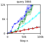
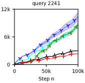
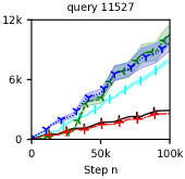
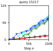
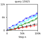
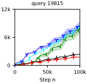
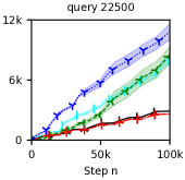
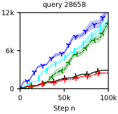
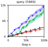
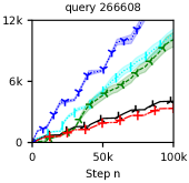
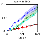
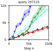
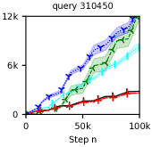
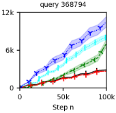
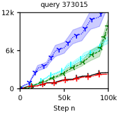
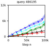
Refer to caption
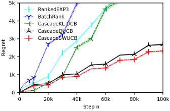
Figure 1: The n-step regret in up to 100100100k steps. Lower is better. The results are averaged over all 100100100 queries and 101010 runs per query. The shaded regions represent standard errors of our estimates.

We report the n𝑛n-step regret averaged over 100100100 queries and 101010 runs per query inΒ FigureΒ 1. All baselines have linear regret in time step. They fail in capturing the breakpoints. Non-stationarity makes the baselines perform even worse during epochs where the attraction probability are set as the default. E.g., π–’π–Ίπ—Œπ–Όπ–Ίπ–½π–Ύπ–ͺπ–«βˆ’π–΄π–’π–‘π–’π–Ίπ—Œπ–Όπ–Ίπ–½π–Ύπ–ͺ𝖫𝖴𝖒𝖑{\sf CascadeKL\mathchar 45\relax UCB} has 111.50Β±1.12plus-or-minus111.501.12111.50\pm 1.12 regret in the first 101010k steps but has 447.82Β±137.16plus-or-minus447.82137.16447.82\pm 137.16 regret between step 808080k and 909090k. Importantly, the attraction probabilities equal the default and remain constant inside these two epochs. This is caused by the fact that the baseline algorithms rank items based on all historical observations, i.e., they do not balance β€œremembering” and β€œforgetting.” Because of the use of a discounting factor and/or a sliding window, π–’π–Ίπ—Œπ–Όπ–Ίπ–½π–Ύπ–£π–΄π–’π–‘π–’π–Ίπ—Œπ–Όπ–Ίπ–½π–Ύπ–£π–΄π–’π–‘{\sf CascadeDUCB} and π–’π–Ίπ—Œπ–Όπ–Ίπ–½π–Ύπ–²π–Άπ–΄π–’π–‘π–’π–Ίπ—Œπ–Όπ–Ίπ–½π–Ύπ–²π–Άπ–΄π–’π–‘{\sf CascadeSWUCB} can detect breakpoints and show convergence. π–’π–Ίπ—Œπ–Όπ–Ίπ–½π–Ύπ–²π–Άπ–΄π–’π–‘π–’π–Ίπ—Œπ–Όπ–Ίπ–½π–Ύπ–²π–Άπ–΄π–’π–‘{\sf CascadeSWUCB} outperforms π–’π–Ίπ—Œπ–Όπ–Ίπ–½π–Ύπ–£π–΄π–’π–‘π–’π–Ίπ—Œπ–Όπ–Ίπ–½π–Ύπ–£π–΄π–’π–‘{\sf CascadeDUCB} with a small gap; this is consistent with our theoretical finding that π–’π–Ίπ—Œπ–Όπ–Ίπ–½π–Ύπ–²π–Άπ–΄π–’π–‘π–’π–Ίπ—Œπ–Όπ–Ίπ–½π–Ύπ–²π–Άπ–΄π–’π–‘{\sf CascadeSWUCB} outperforms π–’π–Ίπ—Œπ–Όπ–Ίπ–½π–Ύπ–£π–΄π–’π–‘π–’π–Ίπ—Œπ–Όπ–Ίπ–½π–Ύπ–£π–΄π–’π–‘{\sf CascadeDUCB} by a ln⁑n𝑛\sqrt{\ln n} factor.

6 Related Work

The idea of directly learning to rank from user feedback has been widely studied in a stationary environment. Ranked banditsΒ Radlinski et al. (2008) are among the earliest OLTR approaches. In ranked bandits, each position in the list is modeled as an individual underlying MABs. The ranking task is then solved by asking each individual MAB to recommend an item to the attached position. Since the reward, e.g., click, of a lower position is affected by higher positions, the underlying MAB is typically adversarial, e.g., 𝖀𝗑𝗉πŸ₯𝖀𝗑𝗉πŸ₯{\sf Exp3}Β Auer et al. (1995). 𝖑𝖺𝗍𝖼𝗁𝖱𝖺𝗇𝗄𝖑𝖺𝗍𝖼𝗁𝖱𝖺𝗇𝗄{\sf BatchRank} is a recently proposed OLTR methodΒ Zoghi et al. (2017); it is an elimination-based algorithm: once an item is found to be inferior to K𝐾K items, it will be removed from future consideration. 𝖑𝖺𝗍𝖼𝗁𝖱𝖺𝗇𝗄𝖑𝖺𝗍𝖼𝗁𝖱𝖺𝗇𝗄{\sf BatchRank} outperforms ranked bandits in the stationary environment. In our experiments, we include 𝖑𝖺𝗍𝖼𝗁𝖱𝖺𝗇𝗄𝖑𝖺𝗍𝖼𝗁𝖱𝖺𝗇𝗄{\sf BatchRank} and 𝖱𝖺𝗇𝗄𝖾𝖽𝖀𝖷𝖯πŸ₯𝖱𝖺𝗇𝗄𝖾𝖽𝖀𝖷𝖯πŸ₯\sf RankedEXP3, the 𝖀𝗑𝗉πŸ₯𝖀𝗑𝗉πŸ₯{\sf Exp3}-based ranked bandit algorithm, as baselines.

Several OLTR algorithms have been proposed in specific click modelsΒ Kveton et al. (2015); LagrΓ©e et al. (2016); Katariya et al. (2016); Oosterhuis and de Rijke (2018). They can efficiently learn an optimal ranking given the click model they consider. Our work is related to cascading bandits and we compare our algorithms to π–’π–Ίπ—Œπ–Όπ–Ίπ–½π–Ύπ–ͺπ–«βˆ’π–΄π–’π–‘π–’π–Ίπ—Œπ–Όπ–Ίπ–½π–Ύπ–ͺ𝖫𝖴𝖒𝖑{\sf CascadeKL\mathchar 45\relax UCB}, an algorithm proposed for soling cascading banditsΒ Kveton et al. (2015), in SectionΒ 5. Our work differs from cascading bandits in that we consider learning in a non-stationary environment.

Non-stationary bandit problems have been widely studiedΒ Slivkins and Upfal (2008); Yu and Mannor (2009); Garivier and Moulines (2011); Besbes et al. (2014); Liu et al. (2018). However, previous work requires a small action space. In our setup, actions are (exponentially many) ranked lists. Thus, we do not consider them as baselines in our experiments.

In adversarial bandits the reward realizations, in our case attraction indicators, are selected by an adversary. Adversarial bandits originate from game theoryΒ Blackwell (1956) and have been widely studied, cf.Β Auer et al. (1995); Cesa-Bianchi and Lugosi (2006) for an overview. Within adversarial bandits, the performance of a policy is often measured by comparing to a static oracle which always chooses a single best arm that is obtained after seeing all the reward realizations up to step n𝑛n. This static oracle can perform poorly in a non-stationary case when the single best arm is suboptimal for a long time between two breakpoints. Thus, even if a policy performs closely to the static oracle, it can still perform sub-optimally in a non-stationary environment. Our work differs from adversarial bandits in that we compare to a dynamic oracle that can balance the dilemma of β€œremembering” and β€œforgetting” and chooses the per-step best action.

7 Conclusion

In this paper, we have studied the online learning to rank (OLTR) problem in a non-stationary environment where user preferences change abruptly. We focus on a widely-used user click behavior model cascade model (CM) and have proposed an online learning variant of it called cascading non-stationary bandtis. Two algorithms, π–’π–Ίπ—Œπ–Όπ–Ίπ–½π–Ύπ–£π–΄π–’π–‘π–’π–Ίπ—Œπ–Όπ–Ίπ–½π–Ύπ–£π–΄π–’π–‘{\sf CascadeDUCB} and π–’π–Ίπ—Œπ–Όπ–Ίπ–½π–Ύπ–²π–Άπ–΄π–’π–‘π–’π–Ίπ—Œπ–Όπ–Ίπ–½π–Ύπ–²π–Άπ–΄π–’π–‘{\sf CascadeSWUCB}, have been proposed for solving it. Our theoretical have shown that they have sub-linear regret. These theoretical findings have been confirmed by our experiments on the Yandex click dataset. We open several future directions for non-stationary OLTR. First, we have only considered the CM setup. Other click models that can handle multiple clicks, e.g., DBNΒ Chapelle and Zhang (2009), should be considered as part of future work. Second, we focused on 𝖴𝖒𝖑𝖴𝖒𝖑{\sf UCB}-based policy. Another possibility is to use the family of softmax policiesΒ Besbes et al. (2014). Along this line, one may obtain upper bounds independent from the number of breakpoints.

Acknowledgements

This research was supported by Ahold Delhaize, the Association of Universities in the Netherlands (VSNU), the Innovation Center for Artificial Intelligence (ICAI), and the Netherlands Organisation for Scientific Research (NWO) under project nr.Β 612.001.551. All content represents the opinion of the authors, which is not necessarily shared or endorsed by their respective employers and/or sponsors.

References

  • Auer et al. [1995] Peter Auer, Nicolo Cesa-Bianchi, Yoav Freund, and Robert Schapire. Gambling in a rigged casino: The adversarial multi-armed bandit problem. In FOCS, pages 322–331, 1995.
  • Auer et al. [2002] Peter Auer, Nicolo Cesa-Bianchi, and Paul Fischer. Finite-time analysis of the multiarmed bandit problem. Machine Learning, 47:235–256, 2002.
  • Besbes et al. [2014] Omar Besbes, Yonatan Gur, and Assaf Zeevi. Stochastic multi-armed-bandit problem with non-stationary rewards. In NIPS, 2014.
  • Blackwell [1956] David Blackwell. An analog of the minimax theorem for vector payoffs. Pacific Journal of Mathematics, 6(1):1–8, November 1956.
  • Cesa-Bianchi and Lugosi [2006] Nicolo Cesa-Bianchi and Gabor Lugosi. Prediction, Learning, and Games. Cambridge University Press, 2006.
  • Chapelle and Zhang [2009] Olivier Chapelle and YaΒ Zhang. A dynamic Bayesian network click model for web search ranking. In WWW, pages 1–10, 2009.
  • Chuklin et al. [2015] Aleksandr Chuklin, Ilya Markov, and Maarten deΒ Rijke. Click Models for Web Search. Morgan & Claypool, 2015.
  • Craswell et al. [2008] Nick Craswell, Onno Zoeter, Michael Taylor, and Bill Ramsey. An experimental comparison of click position-bias models. In WSDM, pages 87–94, 2008.
  • Garivier and Moulines [2008] AurΓ©lien Garivier and Eric Moulines. On upper-confidence bound policies for non-stationary bandit problems. arXiv preprint arXiv:0805.3415, 2008.
  • Garivier and Moulines [2011] AurΓ©lien Garivier and Eric Moulines. On upper-confidence bound policies for switching bandit problems. In ALT, pages 174–188, 2011.
  • Guo et al. [2009] Fan Guo, Chao Liu, and YiΒ Min Wang. Efficient multiple-click models in web search. In WSDM, pages 124–131, 2009.
  • Jagerman et al. [2019] Rolf Jagerman, Ilya Markov, and Maarten deΒ Rijke. When people change their mind: Off-policy evaluation in non-stationary recommendation environments. In WSDM, pages 447–455, 2019.
  • Joachims [2002] Thorsten Joachims. Optimizing search engines using clickthrough data. In SIGKDD, pages 133–142, 2002.
  • Katariya et al. [2016] Sumeet Katariya, Branislav Kveton, Csaba Szepesvari, and Zheng Wen. DCM bandits: Learning to rank with multiple clicks. In ICML, pages 1215–1224, 2016.
  • Kveton et al. [2014] Branislav Kveton, Zheng Wen, Azin Ashkan, Hoda Eydgahi, and Brian Eriksson. Matroid bandits: Fast combinatorial optimization with learning. arXiv preprint arXiv:1403.5045, 2014.
  • Kveton et al. [2015] Branislav Kveton, Csaba Szepesvari, Zheng Wen, and Azin Ashkan. Cascading bandits: Learning to rank in the cascade model. In ICML, pages 767–776, 2015.
  • LagrΓ©e et al. [2016] Paul LagrΓ©e, Claire Vernade, and Olivier Cappe. Multiple-play bandits in the position-based model. In NIPS, 2016.
  • Li et al. [2018] Chang Li, Ilya Markov, Maarten deΒ Rijke, and Masrour Zoghi. Merge double Thompson sampling for large scale online ranker evaluation. arXiv preprint arXiv:1812.04412, 2018.
  • Li et al. [2019] Chang Li, Branislav Kveton, Tor Lattimore, Ilya Markov, Maarten deΒ Rijke, Csaba SzepesvΓ‘ri, and Masrour Zoghi. BubbleRank: Safe online learning to re-rank via implicit click feedback. In UAI, July 2019.
  • Liu et al. [2018] Fang Liu, Joohyun Lee, and Ness Shroff. A change-detection based framework for piecewise-stationary multi-armed bandit problem. In AAAI, pages 3651–3658, 2018.
  • Liu [2009] Tie-Yan Liu. Learning to rank for information retrieval. Foundations and Trends in Information Retrieval, 3(3):225–331, 2009.
  • Oosterhuis and de Rijke [2018] Harrie Oosterhuis and Maarten deΒ Rijke. Differentiable unbiased online learning to rank. In CIKM, pages 1293–1302, 2018.
  • Pereira et al. [2018] FabΓ­olaΒ SF Pereira, JoΓ£o Gama, Sandra deΒ Amo, and GinaΒ MB Oliveira. On analyzing user preference dynamics with temporal social networks. Machine Learning, 107(11):1745–1773, 2018.
  • Qin et al. [2010] Tao Qin, Tie-Yan Liu, Jun Xu, and Hang Li. Letor: A benchmark collection for research on learning to rank for information retrieval. Information Retrieval, 13(4):346–374, 2010.
  • Radlinski et al. [2008] Filip Radlinski, Robert Kleinberg, and Thorsten Joachims. Learning diverse rankings with multi-armed bandits. In ICML, pages 784–791, 2008.
  • Slivkins and Upfal [2008] Aleksandrs Slivkins and Eli Upfal. Adapting to a changing environment: the brownian restless bandits. In COLT, pages 343–354, 2008.
  • Wu et al. [2018] Qingyun Wu, Naveen Iyer, and Hongning Wang. Learning contextual bandits in a non-stationary environment. In SIGIR, pages 495–504, 2018.
  • Yu and Mannor [2009] JiaΒ Yuan Yu and Shie Mannor. Piecewise-stationary bandit problems with side observations. In ICML, 2009.
  • Zoghi et al. [2016] Masrour Zoghi, TomΓ‘Ε‘ Tunys, Lihong Li, Damien Jose, Junyan Chen, ChunΒ Ming Chin, and Maarten deΒ Rijke. Click-based hot fixes for underperforming torso queries. In SIGIR, pages 195–204, 2016.
  • Zoghi et al. [2017] Masrour Zoghi, TomΓ‘Ε‘ Tunys, Mohammad Ghavamzadeh, Branislav Kveton, Csaba Szepesvari, and Zheng Wen. Online learning to rank in stochastic click models. In ICML, pages 4199–4208, 2017.

Appendix A Proofs

In the appendix, we refer to β„›tβˆ—superscriptsubscriptℛ𝑑\mathcal{R}_{t}^{*} as the optimal list at time t𝑑t that includes K𝐾K items sorted by the decreasing order of their attraction probabilities. We refer to π’Ÿtβˆ—βŠ†[L]subscriptsuperscriptπ’Ÿπ‘‘delimited-[]𝐿\mathcal{D}^{*}_{t}\subseteq[L] as the set of the K𝐾K most attractive items in set π’Ÿπ’Ÿ\mathcal{D} at time t𝑑t and π’ŸΒ―tsubscriptΒ―π’Ÿπ‘‘\bar{\mathcal{D}}_{t} as the complement of π’Ÿtβˆ—subscriptsuperscriptπ’Ÿπ‘‘\mathcal{D}^{*}_{t}, i.e. βˆ€aβˆ—βˆˆπ’Ÿtβˆ—,βˆ€aβˆˆπ’ŸΒ―t:Ξ±t​(aβˆ—)β‰₯Ξ±t​(a):formulae-sequencefor-allsuperscriptπ‘Žsuperscriptsubscriptπ’Ÿπ‘‘for-allπ‘ŽsubscriptΒ―π’Ÿπ‘‘subscript𝛼𝑑superscriptπ‘Žsubscriptπ›Όπ‘‘π‘Ž\forall a^{*}\in\mathcal{D}_{t}^{*},\forall a\in\bar{\mathcal{D}}_{t}:\alpha_{t}(a^{*})\geq\alpha_{t}(a) and π’Ÿtβˆ—βˆͺπ’ŸΒ―t=π’Ÿ,π’Ÿtβˆ—βˆ©π’ŸΒ―t=βˆ…formulae-sequencesubscriptsuperscriptπ’Ÿπ‘‘subscriptΒ―π’Ÿπ‘‘π’Ÿsubscriptsuperscriptπ’Ÿπ‘‘subscriptΒ―π’Ÿπ‘‘\mathcal{D}^{*}_{t}\cup\bar{\mathcal{D}}_{t}=\mathcal{D},\mathcal{D}^{*}_{t}\cap\bar{\mathcal{D}}_{t}=\emptyset. At time t𝑑t, we say an item aβˆ—superscriptπ‘Ža^{*} is optimal if aβˆ—βˆˆπ’Ÿtβˆ—superscriptπ‘Žsubscriptsuperscriptπ’Ÿπ‘‘a^{*}\in\mathcal{D}^{*}_{t} and an item aπ‘Ža is suboptimal if aβˆˆπ’ŸΒ―tπ‘ŽsubscriptΒ―π’Ÿπ‘‘a\in\bar{\mathcal{D}}_{t}. We denote 𝐫t=maxR∈ΠK​(π’Ÿ)⁑r​(R,Ξ±t)βˆ’r​(𝐑t,𝐀t)subscript𝐫𝑑subscript𝑅subscriptΞ πΎπ’Ÿπ‘Ÿπ‘…subscriptπ›Όπ‘‘π‘Ÿsubscript𝐑𝑑subscript𝐀𝑑\mathbf{r}_{t}=\max_{R\in\Pi_{K}(\mathcal{D})}r(R,\alpha_{t})-r(\mathbf{R}_{t},\mathbf{A}_{t}) to be the regret at time t𝑑t of the learning algorithm. Let Ξ”a,aβˆ—tsuperscriptsubscriptΞ”π‘Žsuperscriptπ‘Žπ‘‘\Delta_{a,a^{*}}^{t} be the gap of attraction probability between a suboptimal item aπ‘Ža and an optimal aβˆ—superscriptπ‘Ža^{*} at time t𝑑t: Ξ”a,aβˆ—t=Ξ±t​(aβˆ—)βˆ’Ξ±t​(a)superscriptsubscriptΞ”π‘Žsuperscriptπ‘Žπ‘‘subscript𝛼𝑑superscriptπ‘Žsubscriptπ›Όπ‘‘π‘Ž\Delta_{a,a^{*}}^{t}=\alpha_{t}(a^{*})-\alpha_{t}(a). Then we refer to Ξ”a,KsubscriptΞ”π‘ŽπΎ\Delta_{a,K} as the smallest gap between item aπ‘Ža and the K𝐾K-th most attractive item in all n𝑛n time steps when aπ‘Ža is not the optimal item: Ξ”a,K=mint∈[n],aβˆ‰π’Ÿtβˆ—β‘Ξ±t​(K)βˆ’Ξ±t​(a)subscriptΞ”π‘ŽπΎsubscriptformulae-sequence𝑑delimited-[]π‘›π‘Žsubscriptsuperscriptπ’Ÿπ‘‘subscript𝛼𝑑𝐾subscriptπ›Όπ‘‘π‘Ž\Delta_{a,K}=\min_{t\in[n],a\notin\mathcal{D}^{*}_{t}}\alpha_{t}(K)-\alpha_{t}(a).

A.1 Proof of Theorem 1

Let Mt={βˆƒaβˆˆπ’Ÿs.t.|Ξ±t(a)βˆ’πœΆΒ―t(Ξ³,a)|>ct(Ξ³,t)}M_{t}=\{\exists a\in\mathcal{D}~{}s.t.~{}|\alpha_{t}(a)-\bar{\bm{\alpha}}_{t}(\gamma,a)|>c_{t}(\gamma,t)\} be the event that Ξ±t​(a)subscriptπ›Όπ‘‘π‘Ž\alpha_{t}(a) falls out of the confidence interval around 𝜢¯t​(Ξ³,a)subscriptΒ―πœΆπ‘‘π›Ύπ‘Ž\bar{\bm{\alpha}}_{t}(\gamma,a) at time t, and MΒ―tsubscript¯𝑀𝑑\bar{M}_{t} be the complement of Mtsubscript𝑀𝑑{M}_{t}. We re-write the n𝑛n-step regret of π–’π–Ίπ—Œπ–Όπ–Ίπ–½π–Ύπ–£π–΄π–’π–‘π–’π–Ίπ—Œπ–Όπ–Ίπ–½π–Ύπ–£π–΄π–’π–‘{\sf CascadeDUCB} as follows:

R​(n)=𝔼​[βˆ‘t=1nπŸ™β€‹{Mt}​𝐫t]+𝔼​[βˆ‘t=1nπŸ™β€‹{MΒ―t}​𝐫t].𝑅𝑛𝔼delimited-[]superscriptsubscript𝑑1𝑛1subscript𝑀𝑑subscript𝐫𝑑𝔼delimited-[]superscriptsubscript𝑑1𝑛1subscript¯𝑀𝑑subscript𝐫𝑑R(n)=\mathbb{E}\left[{\sum_{t=1}^{n}\mathds{1}\{M_{t}\}\mathbf{r}_{t}}\right]+\mathbb{E}\left[{\sum_{t=1}^{n}\mathds{1}\{\bar{M}_{t}\}\mathbf{r}_{t}}\right]. (21)

We then bound both terms above separated.

We refer to 𝒯𝒯\mathcal{T} as the set of all time steps such that for tβˆˆπ’―π‘‘π’―t\in\mathcal{T}, s∈[tβˆ’B​(Ξ³),t]𝑠𝑑𝐡𝛾𝑑s\in[t-B(\gamma),t] and any item aβˆˆπ’Ÿπ‘Žπ’Ÿa\in\mathcal{D} we have Ξ±s​(a)=Ξ±t​(a)subscriptπ›Όπ‘ π‘Žsubscriptπ›Όπ‘‘π‘Ž\alpha_{s}(a)=\alpha_{t}(a), where B​(Ξ³)=⌈logγ⁑(ϡ​(1βˆ’Ξ³))βŒ‰π΅π›Ύsubscript𝛾italic-Ο΅1𝛾B(\gamma)=\lceil\log_{\gamma}(\epsilon(1-\gamma))\rceil. In other words, 𝒯𝒯\mathcal{T} is the set of time steps that do not follow too close after breakpoints. Since for any time step tβˆ‰π’―π‘‘π’―t\notin\mathcal{T} the estimators of attraction probabilities are biased, π–’π–Ίπ—Œπ–Όπ–Ίπ–½π–Ύπ–£π–΄π–’π–‘π–’π–Ίπ—Œπ–Όπ–Ίπ–½π–Ύπ–£π–΄π–’π–‘{\sf CascadeDUCB} may recommend suboptimal items constantly. Thus, we get the following bound:

𝔼​[βˆ‘t=1nπŸ™β€‹{Mt}​𝐫t]≀L​Ξ₯n​B​(Ξ³)+𝔼​[βˆ‘tβˆˆπ’―πŸ™β€‹{Mt}​𝐫t].𝔼delimited-[]superscriptsubscript𝑑1𝑛1subscript𝑀𝑑subscript𝐫𝑑𝐿subscriptΞ₯𝑛𝐡𝛾𝔼delimited-[]subscript𝑑𝒯1subscript𝑀𝑑subscript𝐫𝑑\mathbb{E}\left[{\sum_{t=1}^{n}\mathds{1}\{M_{t}\}\mathbf{r}_{t}}\right]\leq L\Upsilon_{n}B(\gamma)+\mathbb{E}\left[{\sum_{t\in\mathcal{T}}\mathds{1}\{M_{t}\}\mathbf{r}_{t}}\right]. (22)

Then, we show that for steps tβˆˆπ’―π‘‘π’―t\in\mathcal{T}, the attraction probabilities are well estimated for all items with high probability. For an item aπ‘Ža, we consider the bias and variance of 𝜢¯t​(Ξ³,a)subscriptΒ―πœΆπ‘‘π›Ύπ‘Ž\bar{\bm{\alpha}}_{t}(\gamma,a) separately. We denote:

𝐗t​(Ξ³,a)=βˆ‘s=1tΞ³(tβˆ’s)β€‹πŸ™β€‹{aβˆˆπ‘s,𝐑s​(𝐜s)=a},𝐍t​(Ξ³,a)=βˆ‘s=1tΞ³(tβˆ’s)β€‹πŸ™β€‹{aβˆˆπ‘s},formulae-sequencesubscriptπ—π‘‘π›Ύπ‘Žsuperscriptsubscript𝑠1𝑑superscript𝛾𝑑𝑠1formulae-sequenceπ‘Žsubscript𝐑𝑠subscript𝐑𝑠subscriptπœπ‘ π‘Žsubscriptππ‘‘π›Ύπ‘Žsuperscriptsubscript𝑠1𝑑superscript𝛾𝑑𝑠1π‘Žsubscript𝐑𝑠\mathbf{X}_{t}(\gamma,a)=\sum_{s=1}^{t}\gamma^{(t-s)}\mathds{1}\{a\in\mathbf{R}_{s},\mathbf{R}_{s}(\mathbf{c}_{s})=a\},\quad\mathbf{N}_{t}(\gamma,a)=\sum_{s=1}^{t}\gamma^{(t-s)}\mathds{1}\{a\in\mathbf{R}_{s}\},

as the discounted number of being clicked, and the discounted number of being examined.

First, we consider the bias. The β€œbias” at time t𝑑t can be written as xt​(Ξ³,a)/𝐍t​(Ξ³,a)βˆ’Ξ±tsubscriptπ‘₯π‘‘π›Ύπ‘Žsubscriptππ‘‘π›Ύπ‘Žsubscript𝛼𝑑x_{t}(\gamma,a)/\mathbf{N}_{t}(\gamma,a)-\alpha_{t}, where xt​(Ξ³,a)=βˆ‘s=1tΞ³(tβˆ’s)β€‹πŸ™β€‹{aβˆˆπ‘s}​αs​(a)subscriptπ‘₯π‘‘π›Ύπ‘Žsuperscriptsubscript𝑠1𝑑superscript𝛾𝑑𝑠1π‘Žsubscript𝐑𝑠subscriptπ›Όπ‘ π‘Žx_{t}(\gamma,a)=\sum_{s=1}^{t}\gamma^{(t-s)}\mathds{1}\{a\in\mathbf{R}_{s}\}\alpha_{s}(a). For tβˆˆπ’―π‘‘π’―t\in\mathcal{T}:

|xt​(Ξ³,a)βˆ’Ξ±t​(a)​𝐍t​(Ξ³,a)|subscriptπ‘₯π‘‘π›Ύπ‘Žsubscriptπ›Όπ‘‘π‘Žsubscriptππ‘‘π›Ύπ‘Ž\displaystyle|x_{t}(\gamma,a)-\alpha_{t}(a)\mathbf{N}_{t}(\gamma,a)| =\displaystyle= |βˆ‘s=1tβˆ’B​(Ξ³)Ξ³(tβˆ’s)(Ξ±s(a)βˆ’Ξ±t(a)πŸ™{aβˆˆπ‘t}|\displaystyle\left|\sum_{s=1}^{t-B(\gamma)}\gamma^{(t-s)}(\alpha_{s}(a)-\alpha_{t}(a)\mathds{1}\{a\in\mathbf{R}_{t}\}\right|
≀\displaystyle\leq βˆ‘s=1tβˆ’B​(Ξ³)Ξ³(tβˆ’s)|(Ξ±s(a)βˆ’Ξ±t(a)|πŸ™{aβˆˆπ‘t}\displaystyle\sum_{s=1}^{t-B(\gamma)}\gamma^{(t-s)}\left|(\alpha_{s}(a)-\alpha_{t}(a)\right|\mathds{1}\{a\in\mathbf{R}_{t}\}
≀\displaystyle\leq Ξ³B​(Ξ³)​𝐍tβˆ’B​(Ξ³)​(Ξ³,a)≀γB​(Ξ³)​11βˆ’Ξ³,superscript𝛾𝐡𝛾subscriptππ‘‘π΅π›Ύπ›Ύπ‘Žsuperscript𝛾𝐡𝛾11𝛾\displaystyle\gamma^{B(\gamma)}\mathbf{N}_{t-B(\gamma)}(\gamma,a)\leq\gamma^{B(\gamma)}\frac{1}{1-\gamma},

where the last inequality is due to the fact that 𝐍tβˆ’B​(Ξ³)​(Ξ³,a)≀1/(1βˆ’Ξ³)subscriptππ‘‘π΅π›Ύπ›Ύπ‘Ž11𝛾\mathbf{N}_{t-B(\gamma)}(\gamma,a)\leq 1/(1-\gamma). Thus, we get:

|xt​(Ξ³,a)𝐍t​(Ξ³,a)βˆ’Ξ±t​(a)|subscriptπ‘₯π‘‘π›Ύπ‘Žsubscriptππ‘‘π›Ύπ‘Žsubscriptπ›Όπ‘‘π‘Ž\displaystyle\left|\frac{x_{t}(\gamma,a)}{\mathbf{N}_{t}(\gamma,a)}-\alpha_{t}(a)\right| ≀\displaystyle\leq Ξ³B​(Ξ³)(1βˆ’Ξ³)​𝐍t​(Ξ³,a)≀(1∧γB​(Ξ³)(1βˆ’Ξ³)​𝐍t​(Ξ³,a))superscript𝛾𝐡𝛾1𝛾subscriptππ‘‘π›Ύπ‘Ž1superscript𝛾𝐡𝛾1𝛾subscriptππ‘‘π›Ύπ‘Ž\displaystyle\frac{\gamma^{B(\gamma)}}{(1-\gamma)\mathbf{N}_{t}(\gamma,a)}\leq\left(1\land\frac{\gamma^{B(\gamma)}}{(1-\gamma)\mathbf{N}_{t}(\gamma,a)}\right)
≀\displaystyle\leq Ξ³B​(Ξ³)(1βˆ’Ξ³)​𝐍t​(Ξ³,a)≀ϡ​ln⁑Nt​(Ξ³)𝐍t​(Ξ³,a)≀12​ct​(Ξ³,a),superscript𝛾𝐡𝛾1𝛾subscriptππ‘‘π›Ύπ‘Žitalic-Ο΅subscript𝑁𝑑𝛾subscriptππ‘‘π›Ύπ‘Ž12subscriptπ‘π‘‘π›Ύπ‘Ž\displaystyle\sqrt{\frac{\gamma^{B(\gamma)}}{(1-\gamma)\mathbf{N}_{t}(\gamma,a)}}\leq\sqrt{\frac{\epsilon\ln N_{t}(\gamma)}{\mathbf{N}_{t}(\gamma,a)}}\leq\frac{1}{2}c_{t}(\gamma,a),

where the third inequality is due to the fact that 1∧x≀x1π‘₯π‘₯1\land x\leq\sqrt{x} and the last inequality is due to the definition of B​(Ξ³)𝐡𝛾B(\gamma). So, B​(Ξ³)𝐡𝛾B(\gamma) time steps after a breakpoint, the β€œbias” is at most half as large as the confidence bonus; and the second half of the confidence interval is used for the variance.

Second, we consider the variance. For aβˆˆπ’Ÿπ‘Žπ’Ÿa\in\mathcal{D} and tβˆˆπ’―π‘‘π’―t\in\mathcal{T}, let Mt,a={|Ξ±t​(a)βˆ’πœΆΒ―t​(Ξ³,a)|>ct​(Ξ³,t)}subscriptπ‘€π‘‘π‘Žsubscriptπ›Όπ‘‘π‘ŽsubscriptΒ―πœΆπ‘‘π›Ύπ‘Žsubscript𝑐𝑑𝛾𝑑M_{t,a}=\{|\alpha_{t}(a)-\bar{\bm{\alpha}}_{t}(\gamma,a)|>c_{t}(\gamma,t)\} be the event that Ξ±t​(a)subscriptπ›Όπ‘‘π‘Ž\alpha_{t}(a) falls out of the confidence interval around 𝜢¯t​(Ξ³,a)subscriptΒ―πœΆπ‘‘π›Ύπ‘Ž\bar{\bm{\alpha}}_{t}(\gamma,a) at time t𝑑t. By using a Hoeffding-type inequality ([Garivier and Moulines, 2011, Theorem 4]), for an item aβˆˆπ’Ÿπ‘Žπ’Ÿa\in\mathcal{D}, tβˆˆπ’―π‘‘π’―t\in\mathcal{T}, and any Ξ·>0πœ‚0\eta>0, we get:

P​(Mt,a)𝑃subscriptπ‘€π‘‘π‘Ž\displaystyle P(M_{t,a}) ≀\displaystyle\leq P​(𝐗t​(Ξ³,a)βˆ’xt​(Ξ³,a)𝐍t​(Ξ³2,a)>ϡ​ln⁑Nt​(Ξ³)𝐍t​(Ξ³2,a))𝑃subscriptπ—π‘‘π›Ύπ‘Žsubscriptπ‘₯π‘‘π›Ύπ‘Žsubscript𝐍𝑑superscript𝛾2π‘Žitalic-Ο΅subscript𝑁𝑑𝛾subscript𝐍𝑑superscript𝛾2π‘Ž\displaystyle P\left(\frac{\mathbf{X}_{t}(\gamma,a)-x_{t}(\gamma,a)}{\sqrt{\mathbf{N}_{t}(\gamma^{2},a)}}>\sqrt{\frac{\epsilon\ln N_{t}(\gamma)}{\mathbf{N}_{t}(\gamma^{2},a)}}\right)
≀\displaystyle\leq P​(𝐗t​(Ξ³,a)βˆ’xt​(Ξ³,a)𝐍t​(Ξ³2,a)>ϡ​ln⁑Nt​(Ξ³))𝑃subscriptπ—π‘‘π›Ύπ‘Žsubscriptπ‘₯π‘‘π›Ύπ‘Žsubscript𝐍𝑑superscript𝛾2π‘Žitalic-Ο΅subscript𝑁𝑑𝛾\displaystyle P\left(\frac{\mathbf{X}_{t}(\gamma,a)-x_{t}(\gamma,a)}{\sqrt{\mathbf{N}_{t}(\gamma^{2},a)}}>\sqrt{\epsilon\ln N_{t}(\gamma)}\right)
≀\displaystyle\leq ⌈ln⁑Nt​(Ξ³)ln⁑(1+Ξ·)βŒ‰β€‹Nt​(Ξ³)βˆ’2​ϡ​(1βˆ’Ξ·216).subscript𝑁𝑑𝛾1πœ‚subscript𝑁𝑑superscript𝛾2italic-Ο΅1superscriptπœ‚216\displaystyle\left\lceil\frac{\ln{N_{t}(\gamma)}}{\ln{(1+\eta)}}\right\rceil N_{t}(\gamma)^{-2\epsilon(1-\frac{\eta^{2}}{16})}.

Thus, we get the following bound:

𝔼​[βˆ‘tβˆˆπ’―πŸ™β€‹{Mt}​𝐫t]≀2​Lβ€‹βˆ‘tβˆˆπ’―βŒˆln⁑Nt​(Ξ³)ln⁑(1+Ξ·)βŒ‰β€‹Nt​(Ξ³)βˆ’2​ϡ​(1βˆ’Ξ·216).𝔼delimited-[]subscript𝑑𝒯1subscript𝑀𝑑subscript𝐫𝑑2𝐿subscript𝑑𝒯subscript𝑁𝑑𝛾1πœ‚subscript𝑁𝑑superscript𝛾2italic-Ο΅1superscriptπœ‚216\mathbb{E}\left[{\sum_{t\in\mathcal{T}}\mathds{1}\{M_{t}\}\mathbf{r}_{t}}\right]\leq 2L\sum_{t\in\mathcal{T}}\left\lceil\frac{\ln{N_{t}(\gamma)}}{\ln{(1+\eta)}}\right\rceil N_{t}(\gamma)^{-2\epsilon(1-\frac{\eta^{2}}{16})}.

By taking Ξ·=4​1βˆ’1/2β€‹Ο΅πœ‚4112italic-Ο΅\eta=4\sqrt{1-1/2\epsilon} such that 1βˆ’Ξ·216=11superscriptπœ‚21611-\frac{\eta^{2}}{16}=1, and with t0=(1βˆ’Ξ³)(βˆ’1)subscript𝑑0superscript1𝛾1t_{0}=(1-\gamma)^{(-1)} we get:

βˆ‘tβˆˆπ’―βŒˆln⁑Nt​(Ξ³)ln⁑(1+Ξ·)βŒ‰β€‹Nt​(Ξ³)βˆ’2​ϡ​(1βˆ’Ξ·216)subscript𝑑𝒯subscript𝑁𝑑𝛾1πœ‚subscript𝑁𝑑superscript𝛾2italic-Ο΅1superscriptπœ‚216\displaystyle\sum_{t\in\mathcal{T}}\left\lceil\frac{\ln{N_{t}(\gamma)}}{\ln{(1+\eta)}}\right\rceil N_{t}(\gamma)^{-2\epsilon(1-\frac{\eta^{2}}{16})} ≀\displaystyle\leq t0+βˆ‘tβˆˆπ’―,tβ‰₯t0⌈ln⁑Nt0​(Ξ³)ln⁑(1+Ξ·)βŒ‰β€‹Nt0​(Ξ³)βˆ’1subscript𝑑0subscriptformulae-sequence𝑑𝒯𝑑subscript𝑑0subscript𝑁subscript𝑑0𝛾1πœ‚subscript𝑁subscript𝑑0superscript𝛾1\displaystyle t_{0}+\sum_{t\in\mathcal{T},t\geq t_{0}}\left\lceil\frac{\ln{N_{t_{0}}(\gamma)}}{\ln{(1+\eta)}}\right\rceil N_{t_{0}}(\gamma)^{-1}
≀\displaystyle\leq t0+⌈ln⁑Nt0​(Ξ³)ln⁑(1+Ξ·)βŒ‰β€‹nNt0​(Ξ³)subscript𝑑0subscript𝑁subscript𝑑0𝛾1πœ‚π‘›subscript𝑁subscript𝑑0𝛾\displaystyle t_{0}+\left\lceil\frac{\ln{N_{t_{0}}(\gamma)}}{\ln{(1+\eta)}}\right\rceil\frac{n}{N_{t_{0}}(\gamma)}
≀\displaystyle\leq 11βˆ’Ξ³+⌈ln⁑Nt0​(Ξ³)ln⁑(1+Ξ·)βŒ‰β€‹n​(1βˆ’Ξ³)1βˆ’Ξ³1/(1βˆ’Ξ³).11𝛾subscript𝑁subscript𝑑0𝛾1πœ‚π‘›1𝛾1superscript𝛾11𝛾\displaystyle\frac{1}{1-\gamma}+\left\lceil\frac{\ln{N_{t_{0}}(\gamma)}}{\ln{(1+\eta)}}\right\rceil\frac{n(1-\gamma)}{1-\gamma^{1/(1-\gamma)}}.

We sum up and get the upper bound:

𝔼​[βˆ‘t=1nπŸ™β€‹{MΒ―t}​𝐫t]≀L​Ξ₯n​B​(Ξ³)+2​L​11βˆ’Ξ³+2​Lβ€‹βŒˆln⁑Nt0​(Ξ³)ln⁑(1+Ξ·)βŒ‰β€‹n​(1βˆ’Ξ³)1βˆ’Ξ³1/(1βˆ’Ξ³).𝔼delimited-[]superscriptsubscript𝑑1𝑛1subscript¯𝑀𝑑subscript𝐫𝑑𝐿subscriptΞ₯𝑛𝐡𝛾2𝐿11𝛾2𝐿subscript𝑁subscript𝑑0𝛾1πœ‚π‘›1𝛾1superscript𝛾11𝛾\mathbb{E}\left[{\sum_{t=1}^{n}\mathds{1}\{\bar{M}_{t}\}\mathbf{r}_{t}}\right]\leq L\Upsilon_{n}B(\gamma)+2L\frac{1}{1-\gamma}+2L\left\lceil\frac{\ln{N_{t_{0}}(\gamma)}}{\ln{(1+\eta)}}\right\rceil\frac{n(1-\gamma)}{1-\gamma^{1/(1-\gamma)}}. (23)

Third, we upper bound the second term in Eq.Β 21. The regret is caused by recommending a suboptimal item to the user and the user examines but does not click the item. Since there are Ξ₯nsubscriptΞ₯𝑛\Upsilon_{n} breakpoints, we refer to [t1,…,tΞ₯n]subscript𝑑1…subscript𝑑subscriptΞ₯𝑛[t_{1},\ldots,t_{\Upsilon_{n}}] as the time step of a breakpoint that occurs. We consider the time step in the individual epoch that does not contain a breakpoint. For any epoch and any time t∈{te,te+1,…,te+1βˆ’1}𝑑subscript𝑑𝑒subscript𝑑𝑒1…subscript𝑑𝑒11t\in\{t_{e},t_{e}+1,\ldots,t_{e+1}-1\}, any item aβˆˆπ’ŸΒ―eπ‘ŽsubscriptΒ―π’Ÿπ‘’a\in\bar{\mathcal{D}}_{e} and any item aβˆ—βˆˆπ’Ÿeβˆ—superscriptπ‘Žsubscriptsuperscriptπ’Ÿπ‘’a^{*}\in\mathcal{D}^{*}_{e}, we define the event that item aπ‘Ža is included in 𝐑tsubscript𝐑𝑑\mathbf{R}_{t} instead of item aβˆ—superscriptπ‘Ža^{*}, and item aπ‘Ža is examined but not clicked at time t𝑑t by:

Gt,a,aβˆ—={βˆƒ1≀k<𝐜ts.t.𝐑t(k)=a,β„›t(k)=aβˆ—}.\begin{split}G_{t,a,a^{*}}=\{\exists 1\leq k<\mathbf{c}_{t}~{}s.t.~{}\mathbf{R}_{t}(k)=a,\mathcal{R}_{t}(k)=a^{*}\}.\end{split}

Since the attraction probability remains constant in the epoch, we refer to π’Ÿeβˆ—subscriptsuperscriptπ’Ÿπ‘’\mathcal{D}^{*}_{e} as the optimal items and π’ŸΒ―esubscriptΒ―π’Ÿπ‘’\bar{\mathcal{D}}_{e} as the suboptimal items in epoch e𝑒e. By [Kveton et al., 2015, Theorem 1], the regret at time t𝑑t is decomposed as:

𝔼​[𝐫t]≀Δa,aβˆ—tβ€‹βˆ‘aβˆˆπ’ŸΒ―eβˆ‘aβ£βˆ—β£βˆˆπ’Ÿeβˆ—πŸ™β€‹{Ga,aβˆ—,t}.𝔼delimited-[]subscript𝐫𝑑subscriptsuperscriptΞ”π‘‘π‘Žsuperscriptπ‘Žsubscriptπ‘ŽsubscriptΒ―π’Ÿπ‘’subscriptπ‘Žabsentsubscriptsuperscriptπ’Ÿπ‘’1subscriptπΊπ‘Žsuperscriptπ‘Žπ‘‘\mathbb{E}[\mathbf{r}_{t}]\leq\Delta^{t}_{a,a^{*}}\sum_{a\in\bar{\mathcal{D}}_{e}}\sum_{a*\in\mathcal{D}^{*}_{e}}\mathds{1}\{G_{a,a^{*},t}\}. (24)

Then we have:

𝔼​[βˆ‘t=titi+1βˆ’1πŸ™β€‹{MΒ―t}​𝐫t]=βˆ‘t=titi+1βˆ’1πŸ™β€‹{MΒ―t}​𝔼​[𝐫t]β‰€βˆ‘aβˆˆπ’ŸΒ―e𝔼​[βˆ‘aβˆ—βˆˆπ’Ÿeβˆ—βˆ‘t=titi+1βˆ’1Ξ”a,aβˆ—tβ€‹πŸ™β€‹{Ga,aβˆ—,t}],𝔼delimited-[]superscriptsubscript𝑑subscript𝑑𝑖subscript𝑑𝑖111subscript¯𝑀𝑑subscript𝐫𝑑superscriptsubscript𝑑subscript𝑑𝑖subscript𝑑𝑖111subscript¯𝑀𝑑𝔼delimited-[]subscript𝐫𝑑subscriptπ‘ŽsubscriptΒ―π’Ÿπ‘’π”Όdelimited-[]subscriptsuperscriptπ‘Žsubscriptsuperscriptπ’Ÿπ‘’superscriptsubscript𝑑subscript𝑑𝑖subscript𝑑𝑖11subscriptsuperscriptΞ”π‘‘π‘Žsuperscriptπ‘Ž1subscriptπΊπ‘Žsuperscriptπ‘Žπ‘‘\mathbb{E}\left[{\sum_{t=t_{i}}^{t_{i+1}-1}\mathds{1}\{\bar{M}_{t}\}\mathbf{r}_{t}}\right]=\sum_{t=t_{i}}^{t_{i+1}-1}\mathds{1}\{\bar{M}_{t}\}\mathbb{E}\left[{\mathbf{r}_{t}}\right]\leq\sum_{a\in\bar{\mathcal{D}}_{e}}\mathbb{E}\left[{\sum_{a^{*}\in\mathcal{D}^{*}_{e}}\sum_{t=t_{i}}^{t_{i+1}-1}\Delta^{t}_{a,a^{*}}\mathds{1}\{G_{a,a^{*},t}\}}\right], (25)

where the first equality is due to the tower rule, and the inequality is due to Eq.Β 24.

Now, for any suboptimal item aπ‘Ža in epoch e𝑒e, we upper bound 𝔼​[βˆ‘aβˆ—βˆˆπ’Ÿeβˆ—βˆ‘t=titi+1βˆ’1Ξ”a,aβˆ—tβ€‹πŸ™β€‹{Ga,aβˆ—,t}]𝔼delimited-[]subscriptsuperscriptπ‘Žsubscriptsuperscriptπ’Ÿπ‘’superscriptsubscript𝑑subscript𝑑𝑖subscript𝑑𝑖11subscriptsuperscriptΞ”π‘‘π‘Žsuperscriptπ‘Ž1subscriptπΊπ‘Žsuperscriptπ‘Žπ‘‘\mathbb{E}\left[{\sum_{a^{*}\in\mathcal{D}^{*}_{e}}\sum_{t=t_{i}}^{t_{i+1}-1}\Delta^{t}_{a,a^{*}}\mathds{1}\{G_{a,a^{*},t}\}}\right]. At time t𝑑t, event πŸ™β€‹{MΒ―t}1subscript¯𝑀𝑑\mathds{1}\{\bar{M}_{t}\} and event πŸ™β€‹{aβˆˆπ‘t,aβˆˆπ’ŸΒ―t}1formulae-sequenceπ‘Žsubscriptπ‘π‘‘π‘ŽsubscriptΒ―π’Ÿπ‘‘\mathds{1}\{a\in\mathbf{R}_{t},a\in\bar{\mathcal{D}}_{t}\} happen when there exists an optimal item aβˆ—βˆˆπ’Ÿeβˆ—superscriptπ‘Žsubscriptsuperscriptπ’Ÿπ‘’a^{*}\in\mathcal{D}^{*}_{e} such that:

Ξ±t​(a)+2​ct​(Ξ³,a)β‰₯𝐔t​(a)β‰₯𝐔​(aβˆ—)β‰₯Ξ±t​(aβˆ—),subscriptπ›Όπ‘‘π‘Ž2subscriptπ‘π‘‘π›Ύπ‘Žsubscriptπ”π‘‘π‘Žπ”superscriptπ‘Žsubscript𝛼𝑑superscriptπ‘Ž\alpha_{t}(a)+2c_{t}(\gamma,a)\geq\mathbf{U}_{t}(a)\geq\mathbf{U}(a^{*})\geq\alpha_{t}(a^{*}),

which implies that 2​ct​(Ξ³,a)β‰₯Ξ±t​(aβˆ—)βˆ’Ξ±t​(a)2subscriptπ‘π‘‘π›Ύπ‘Žsubscript𝛼𝑑superscriptπ‘Žsubscriptπ›Όπ‘‘π‘Ž2c_{t}(\gamma,a)\geq\alpha_{t}(a^{*})-\alpha_{t}(a). Taking the definition of the confidence interval, we get:

𝐍t​(Ξ³,a)≀16​ϡ​ln⁑Nt​(Ξ³)Ξ”t,a,aβˆ—2,subscriptππ‘‘π›Ύπ‘Ž16italic-Ο΅subscript𝑁𝑑𝛾subscriptsuperscriptΞ”2π‘‘π‘Žsuperscriptπ‘Ž\mathbf{N}_{t}(\gamma,a)\leq\frac{16\epsilon\ln N_{t}(\gamma)}{\Delta^{2}_{t,a,a^{*}}},

where we set Ξ”t,a,aβˆ—=Ξ”a,aβˆ—tsubscriptΞ”π‘‘π‘Žsuperscriptπ‘ŽsubscriptsuperscriptΞ”π‘‘π‘Žsuperscriptπ‘Ž\Delta_{t,a,a^{*}}=\Delta^{t}_{a,a^{*}}.

Together with Eq.Β 25, we get:

𝔼​[βˆ‘t=titi+1βˆ’1πŸ™β€‹{MΒ―t}​𝐫t]𝔼delimited-[]superscriptsubscript𝑑subscript𝑑𝑖subscript𝑑𝑖111subscript¯𝑀𝑑subscript𝐫𝑑\displaystyle\mathbb{E}\left[{\sum_{t=t_{i}}^{t_{i+1}-1}\mathds{1}\{\bar{M}_{t}\}\mathbf{r}_{t}}\right] ≀\displaystyle\leq βˆ‘aβˆˆπ’ŸΒ―e𝔼​[βˆ‘aβˆ—βˆˆπ’Ÿeβˆ—16​ϡ​ln⁑Nt​(Ξ³)Ξ”t,a,aβˆ—]subscriptπ‘ŽsubscriptΒ―π’Ÿπ‘’π”Όdelimited-[]subscriptsuperscriptπ‘Žsubscriptsuperscriptπ’Ÿπ‘’16italic-Ο΅subscript𝑁𝑑𝛾subscriptΞ”π‘‘π‘Žsuperscriptπ‘Ž\displaystyle\sum_{a\in\bar{\mathcal{D}}_{e}}\mathbb{E}\left[{\sum_{a^{*}\in\mathcal{D}^{*}_{e}}\frac{16\epsilon\ln N_{t}(\gamma)}{\Delta_{t,a,a^{*}}}}\right] (26)
≀\displaystyle\leq 16​ϡ​ln⁑Nt​(Ξ³)​[Ξ”t,a,1​1Ξ”t,a,12+βˆ‘aβˆ—=2KΞ”t,a,aβˆ—β€‹(1Ξ”t,a,aβˆ—2βˆ’1Ξ”t,a,aβˆ—βˆ’12)]16italic-Ο΅subscript𝑁𝑑𝛾delimited-[]subscriptΞ”π‘‘π‘Ž11subscriptsuperscriptΞ”2π‘‘π‘Ž1superscriptsubscriptsuperscriptπ‘Ž2𝐾subscriptΞ”π‘‘π‘Žsuperscriptπ‘Ž1subscriptsuperscriptΞ”2π‘‘π‘Žsuperscriptπ‘Ž1subscriptsuperscriptΞ”2π‘‘π‘Žsuperscriptπ‘Ž1\displaystyle 16\epsilon\ln N_{t}(\gamma)\left[\Delta_{t,a,1}\frac{1}{\Delta^{2}_{t,a,1}}+\sum_{a^{*}=2}^{K}\Delta_{t,a,a^{*}}\left(\frac{1}{\Delta^{2}_{t,a,a^{*}}}-\frac{1}{\Delta^{2}_{t,a,a^{*}-1}}\right)\right]
≀\displaystyle\leq 32​ϡ​ln⁑Nt​(Ξ³)Ξ”t,a,K,32italic-Ο΅subscript𝑁𝑑𝛾subscriptΞ”π‘‘π‘ŽπΎ\displaystyle\frac{32\epsilon\ln N_{t}(\gamma)}{\Delta_{t,a,K}},

where the last inequality is due to [Kveton et al., 2014, Lemma 3]. Let Ξ”a,K=mint∈[n]⁑Δt,a,KsubscriptΞ”π‘ŽπΎsubscript𝑑delimited-[]𝑛subscriptΞ”π‘‘π‘ŽπΎ\Delta_{a,K}=\min_{t\in[n]}\Delta_{t,a,K} be the smallest gap between the suboptimal item aπ‘Ža and an optimal item in all time steps. When 𝐍t​(Ξ³,a)>32​ϡ​ln⁑Nt​(Ξ³)Ξ”a,K2subscriptππ‘‘π›Ύπ‘Ž32italic-Ο΅subscript𝑁𝑑𝛾subscriptsuperscriptΞ”2π‘ŽπΎ\mathbf{N}_{t}(\gamma,a)>\frac{32\epsilon\ln N_{t}(\gamma)}{\Delta^{2}_{a,K}}, π–’π–Ίπ—Œπ–Όπ–Ίπ–½π–Ύπ–£π–΄π–’π–‘π–’π–Ίπ—Œπ–Όπ–Ίπ–½π–Ύπ–£π–΄π–’π–‘{\sf CascadeDUCB} will not select item aπ‘Ža at time t𝑑t. Thus we get:

βˆ‘aβˆˆπ’Ÿπ”Όβ€‹[βˆ‘t=1nπŸ™β€‹{MΒ―t}β€‹πŸ™β€‹{aβˆˆπ‘t,aβˆˆπ’ŸΒ―t}]subscriptπ‘Žπ’Ÿπ”Όdelimited-[]superscriptsubscript𝑑1𝑛1subscript¯𝑀𝑑1formulae-sequenceπ‘Žsubscriptπ‘π‘‘π‘ŽsubscriptΒ―π’Ÿπ‘‘\displaystyle\sum_{a\in\mathcal{D}}\mathbb{E}\left[{\sum_{t=1}^{n}\mathds{1}\{\bar{M}_{t}\}\mathds{1}\{a\in\mathbf{R}_{t},a\in\bar{\mathcal{D}}_{t}\}}\right] ≀\displaystyle\leq βˆ‘e∈[Ξ₯n]βˆ‘aβˆˆπ’ŸΒ―e32​ϡ​ln⁑Nt​(Ξ³)Ξ”t,a,Ksubscript𝑒delimited-[]subscriptΞ₯𝑛subscriptπ‘ŽsubscriptΒ―π’Ÿπ‘’32italic-Ο΅subscript𝑁𝑑𝛾subscriptΞ”π‘‘π‘ŽπΎ\displaystyle\sum_{e\in[\Upsilon_{n}]}\sum_{a\in\bar{\mathcal{D}}_{e}}\frac{32\epsilon\ln N_{t}(\gamma)}{\Delta_{t,a,K}} (27)
≀\displaystyle\leq βˆ‘aβˆˆπ’ŸβŒˆn​(1βˆ’Ξ³)βŒ‰β€‹32​ϡ​ln⁑Nn​(Ξ³)Ξ”a,K​γ1/(1βˆ’Ξ³),subscriptπ‘Žπ’Ÿπ‘›1𝛾32italic-Ο΅subscript𝑁𝑛𝛾subscriptΞ”π‘ŽπΎsuperscript𝛾11𝛾\displaystyle\sum_{a\in\mathcal{D}}\lceil n(1-\gamma)\rceil\frac{32\epsilon\ln N_{n}(\gamma)}{\Delta_{a,K}}\gamma^{1/(1-\gamma)},

where the last inequality is based on [Garivier and Moulines, 2011, Lemma 1].

Finally, together with Eq.Β 21, Eq.Β 22, Eq.Β 23, Eq.Β 24, Eq.Β 25 and Eq.Β 27, we get TheoremΒ 1.

A.2 Proof of Theorem 2

Let Mt={βˆƒaβˆˆπ’Ÿs.t.|Ξ±t(a)βˆ’πœΆΒ―t(Ο„,a)|>ct(Ο„,t)}M_{t}=\{\exists a\in\mathcal{D}~{}s.t.~{}|\alpha_{t}(a)-\bar{\bm{\alpha}}_{t}(\tau,a)|>c_{t}(\tau,t)\} be the event that Ξ±t​(a)subscriptπ›Όπ‘‘π‘Ž\alpha_{t}(a) falls out of the confidence interval around 𝜢¯t​(Ο„,a)subscriptΒ―πœΆπ‘‘πœπ‘Ž\bar{\bm{\alpha}}_{t}(\tau,a) at time t, and let MΒ―tsubscript¯𝑀𝑑\bar{M}_{t} be the complement of Mtsubscript𝑀𝑑{M}_{t}. We re-write the n𝑛n-step regret of π–’π–Ίπ—Œπ–Όπ–Ίπ–½π–Ύπ–²π–Άπ–΄π–’π–‘π–’π–Ίπ—Œπ–Όπ–Ίπ–½π–Ύπ–²π–Άπ–΄π–’π–‘{\sf CascadeSWUCB} as follows:

R​(n)=𝔼​[βˆ‘t=1nπŸ™β€‹{Mt}​𝐫t]+𝔼​[βˆ‘t=1nπŸ™β€‹{MΒ―t}​𝐫t].𝑅𝑛𝔼delimited-[]superscriptsubscript𝑑1𝑛1subscript𝑀𝑑subscript𝐫𝑑𝔼delimited-[]superscriptsubscript𝑑1𝑛1subscript¯𝑀𝑑subscript𝐫𝑑R(n)=\mathbb{E}\left[{\sum_{t=1}^{n}\mathds{1}\{M_{t}\}\mathbf{r}_{t}}\right]+\mathbb{E}\left[{\sum_{t=1}^{n}\mathds{1}\{\bar{M}_{t}\}\mathbf{r}_{t}}\right]. (28)

We then bound both terms in Eq.Β 28 separately.

First, we refer to 𝒯𝒯\mathcal{T} as the set of all time steps such that for tβˆˆπ’―π‘‘π’―t\in\mathcal{T}, s∈[tβˆ’Ο„,t]π‘ π‘‘πœπ‘‘s\in[t-\tau,t] and any item aβˆˆπ’Ÿπ‘Žπ’Ÿa\in\mathcal{D} we have Ξ±s​(a)=Ξ±t​(a)subscriptπ›Όπ‘ π‘Žsubscriptπ›Όπ‘‘π‘Ž\alpha_{s}(a)=\alpha_{t}(a). In other words, 𝒯𝒯\mathcal{T} is the set of time steps that do not follow too close after breakpoints. Obviously, for any time step tβˆ‰π’―π‘‘π’―t\notin\mathcal{T} the estimators of attraction probabilities are biased and π–’π–Ίπ—Œπ–Όπ–Ίπ–½π–Ύπ–²π–Άπ–΄π–’π–‘π–’π–Ίπ—Œπ–Όπ–Ίπ–½π–Ύπ–²π–Άπ–΄π–’π–‘{\sf CascadeSWUCB} may recommend suboptimal items constantly. Thus, we get the following bound:

𝔼​[βˆ‘t=1nπŸ™β€‹{Mt}​𝐫t]≀L​Ξ₯n​τ+𝔼​[βˆ‘tβˆˆπ’―πŸ™β€‹{Mt}​𝐫t].𝔼delimited-[]superscriptsubscript𝑑1𝑛1subscript𝑀𝑑subscript𝐫𝑑𝐿subscriptΞ₯π‘›πœπ”Όdelimited-[]subscript𝑑𝒯1subscript𝑀𝑑subscript𝐫𝑑\mathbb{E}\left[{\sum_{t=1}^{n}\mathds{1}\{M_{t}\}\mathbf{r}_{t}}\right]\leq L\Upsilon_{n}\tau+\mathbb{E}\left[{\sum_{t\in\mathcal{T}}\mathds{1}\{M_{t}\}\mathbf{r}_{t}}\right]. (29)

Ο„πœ\tau time steps after a breakpoint, the estimators of the attraction probabilities are not biased.

Then, we consider the variance. By using a Hoeffding-type inequality ([Garivier and Moulines, 2008, Corollary 21]), for an item aβˆˆπ’Ÿπ‘Žπ’Ÿa\in\mathcal{D}, tβˆˆπ’―π‘‘π’―t\in\mathcal{T}, and any Ξ·>0πœ‚0\eta>0, we get:

P​(|𝜢¯t​(Ο„,a)βˆ’Ξ±t​(a)|>ct​(Ο„,t))𝑃subscriptΒ―πœΆπ‘‘πœπ‘Žsubscriptπ›Όπ‘‘π‘Žsubscriptπ‘π‘‘πœπ‘‘\displaystyle P\left(\left|\bar{\bm{\alpha}}_{t}(\tau,a)-\alpha_{t}(a)\right|>c_{t}(\tau,t)\right) ≀\displaystyle\leq P​(𝜢¯t​(Ο„,a)>Ξ±t​(a)+ϡ​ln⁑(tβˆ§Ο„)𝐍t​(Ο„,a))+P​(𝜢¯t​(Ο„,a)<Ξ±t​(a)βˆ’Ο΅β€‹ln⁑(tβˆ§Ο„)𝐍t​(Ο„,a))𝑃subscriptΒ―πœΆπ‘‘πœπ‘Žsubscriptπ›Όπ‘‘π‘Žitalic-Ο΅π‘‘πœsubscriptππ‘‘πœπ‘Žπ‘ƒsubscriptΒ―πœΆπ‘‘πœπ‘Žsubscriptπ›Όπ‘‘π‘Žitalic-Ο΅π‘‘πœsubscriptππ‘‘πœπ‘Ž\displaystyle P\left(\bar{\bm{\alpha}}_{t}(\tau,a)>\alpha_{t}(a)+\sqrt{\frac{\epsilon\ln{(t\land\tau)}}{\mathbf{N}_{t}(\tau,a)}}\right)+P\left(\bar{\bm{\alpha}}_{t}(\tau,a)<\alpha_{t}(a)-\sqrt{\frac{\epsilon\ln{(t\land\tau)}}{\mathbf{N}_{t}(\tau,a)}}\right)
≀\displaystyle\leq 2β€‹βŒˆln⁑(tβˆ§Ο„)ln⁑(1+Ξ·)βŒ‰β€‹exp⁑(βˆ’2​ϡ​ln⁑(tβˆ§Ο„)​(1βˆ’Ξ·16))2π‘‘πœ1πœ‚2italic-Ο΅π‘‘πœ1πœ‚16\displaystyle 2\left\lceil\frac{\ln{(t\land\tau)}}{\ln(1+\eta)}\right\rceil\exp\left(-2\epsilon\ln(t\land\tau)(1-\frac{\eta}{16})\right)
=\displaystyle= 2β€‹βŒˆln⁑(tβˆ§Ο„)ln⁑(1+Ξ·)βŒ‰β€‹(tβˆ§Ο„)βˆ’2​ϡ​(1βˆ’Ξ·2/16).2π‘‘πœ1πœ‚superscriptπ‘‘πœ2italic-Ο΅1superscriptπœ‚216\displaystyle 2\left\lceil\frac{\ln{(t\land\tau)}}{\ln(1+\eta)}\right\rceil(t\land\tau)^{-2\epsilon(1-\eta^{2}/16)}.

Taking Ξ·=4​1βˆ’12β€‹Ο΅πœ‚4112italic-Ο΅\eta=4\sqrt{1-\frac{1}{2\epsilon}}, we have: P​(|𝜢¯t​(Ο„,a)βˆ’Ξ±t​(a)|)≀2β€‹βŒˆln⁑(tβˆ§Ο„)ln⁑(1+Ξ·)βŒ‰tβˆ§Ο„.𝑃subscriptΒ―πœΆπ‘‘πœπ‘Žsubscriptπ›Όπ‘‘π‘Ž2π‘‘πœ1πœ‚π‘‘πœP\left(\left|\bar{\bm{\alpha}}_{t}(\tau,a)-\alpha_{t}(a)\right|\right)\leq 2\frac{\left\lceil\frac{\ln{(t\land\tau)}}{\ln(1+\eta)}\right\rceil}{t\land\tau}. Thus, we get the following bound:

𝔼​[βˆ‘tβˆˆπ’―πŸ™β€‹{Mt}​𝐫t]≀2​Lβ€‹βˆ‘tβˆˆπ’―βŒˆln⁑(tβˆ§Ο„)ln⁑(1+Ξ·)βŒ‰tβˆ§Ο„β‰€L​ln2⁑(Ο„)ln(1+41βˆ’1/2Ο΅)+2​L​n​ln⁑ττ​ln⁑(1+4​1βˆ’1/2​ϡ).\mathbb{E}\left[{\sum_{t\in\mathcal{T}}\mathds{1}\{M_{t}\}\mathbf{r}_{t}}\right]\leq 2L\sum_{t\in\mathcal{T}}\frac{\left\lceil\frac{\ln{(t\land\tau)}}{\ln(1+\eta)}\right\rceil}{t\land\tau}\leq\frac{L\ln^{2}(\tau)}{\ln(1+4\sqrt{1-1/2\epsilon)}}+\frac{2Ln\ln\tau}{\tau\ln(1+4\sqrt{1-1/2\epsilon})}.

We sum up and get the upper bound:

𝔼​[βˆ‘t=1nπŸ™β€‹{MΒ―t}​𝐑t]≀L​Ξ₯n​τ+L​ln2⁑(Ο„)ln(1+41βˆ’1/2Ο΅)+2​L​n​ln⁑ττ​ln⁑(1+4​1βˆ’1/2​ϡ).\mathbb{E}\left[{\sum_{t=1}^{n}\mathds{1}\{\bar{M}_{t}\}\mathbf{R}_{t}}\right]\leq L\Upsilon_{n}\tau+\frac{L\ln^{2}(\tau)}{\ln(1+4\sqrt{1-1/2\epsilon)}}+\frac{2Ln\ln\tau}{\tau\ln(1+4\sqrt{1-1/2\epsilon})}. (30)

Third, we upper bound the second term in Eq.Β 28. The regret is caused by recommending a suboptimal item to the user and the user examines but does not click the item. Since there are Ξ₯nsubscriptΞ₯𝑛\Upsilon_{n} breakpoints, we refer to [t1,…,tΞ₯n]subscript𝑑1…subscript𝑑subscriptΞ₯𝑛[t_{1},\ldots,t_{\Upsilon_{n}}] as the time steps of a breakpoint. We consider the time step in the individual epoch that does not contain a breakpoint. For any epoch and any time t∈{te,te+1,…,te+1βˆ’1}𝑑subscript𝑑𝑒subscript𝑑𝑒1…subscript𝑑𝑒11t\in\{t_{e},t_{e}+1,\ldots,t_{e+1}-1\}, any item aβˆˆπ’ŸΒ―eπ‘ŽsubscriptΒ―π’Ÿπ‘’a\in\bar{\mathcal{D}}_{e} and any item aβˆ—βˆˆπ’Ÿeβˆ—superscriptπ‘Žsubscriptsuperscriptπ’Ÿπ‘’a^{*}\in\mathcal{D}^{*}_{e}, we define the event that item aπ‘Ža is included in 𝐑tsubscript𝐑𝑑\mathbf{R}_{t} instead of item aβˆ—superscriptπ‘Ža^{*} and item aπ‘Ža is examined but not clicked at time t𝑑t by:

Gt,a,aβˆ—={βˆƒ1≀k<𝐜ts.t.𝐑t(k)=a,β„›t(k)=aβˆ—}.\begin{split}G_{t,a,a^{*}}=\{\exists 1\leq k<\mathbf{c}_{t}~{}s.t.~{}\mathbf{R}_{t}(k)=a,\mathcal{R}_{t}(k)=a^{*}\}.\end{split}

Since the attraction probabilities remain constant in the epoch, we refer to π’Ÿeβˆ—subscriptsuperscriptπ’Ÿπ‘’\mathcal{D}^{*}_{e} as the optimal items and π’ŸΒ―esubscriptΒ―π’Ÿπ‘’\bar{\mathcal{D}}_{e} as the suboptimal items in epoch e𝑒e. By [Kveton et al., 2015, Theorem 1], the regret at time t𝑑t is decomposed as:

𝔼​[𝐫t]≀Δa,aβˆ—tβ€‹βˆ‘aβˆˆπ’ŸΒ―eβˆ‘aβ£βˆ—β£βˆˆπ’Ÿeβˆ—πŸ™β€‹{Ga,aβˆ—,t}.𝔼delimited-[]subscript𝐫𝑑subscriptsuperscriptΞ”π‘‘π‘Žsuperscriptπ‘Žsubscriptπ‘ŽsubscriptΒ―π’Ÿπ‘’subscriptπ‘Žabsentsubscriptsuperscriptπ’Ÿπ‘’1subscriptπΊπ‘Žsuperscriptπ‘Žπ‘‘\mathbb{E}[\mathbf{r}_{t}]\leq\Delta^{t}_{a,a^{*}}\sum_{a\in\bar{\mathcal{D}}_{e}}\sum_{a*\in\mathcal{D}^{*}_{e}}\mathds{1}\{G_{a,a^{*},t}\}. (31)

Then we have:

𝔼​[βˆ‘t=titi+1βˆ’1πŸ™β€‹{MΒ―t}​𝐫t]=βˆ‘t=titi+1βˆ’1πŸ™β€‹{MΒ―t}​𝔼​[𝐫t]β‰€βˆ‘aβˆˆπ’ŸΒ―e𝔼​[βˆ‘aβˆ—βˆˆπ’Ÿeβˆ—βˆ‘t=titi+1βˆ’1Ξ”a,aβˆ—tβ€‹πŸ™β€‹{Ga,aβˆ—,t}],𝔼delimited-[]superscriptsubscript𝑑subscript𝑑𝑖subscript𝑑𝑖111subscript¯𝑀𝑑subscript𝐫𝑑superscriptsubscript𝑑subscript𝑑𝑖subscript𝑑𝑖111subscript¯𝑀𝑑𝔼delimited-[]subscript𝐫𝑑subscriptπ‘ŽsubscriptΒ―π’Ÿπ‘’π”Όdelimited-[]subscriptsuperscriptπ‘Žsubscriptsuperscriptπ’Ÿπ‘’superscriptsubscript𝑑subscript𝑑𝑖subscript𝑑𝑖11subscriptsuperscriptΞ”π‘‘π‘Žsuperscriptπ‘Ž1subscriptπΊπ‘Žsuperscriptπ‘Žπ‘‘\mathbb{E}\left[{\sum_{t=t_{i}}^{t_{i+1}-1}\mathds{1}\{\bar{M}_{t}\}\mathbf{r}_{t}}\right]=\sum_{t=t_{i}}^{t_{i+1}-1}\mathds{1}\{\bar{M}_{t}\}\mathbb{E}\left[{\mathbf{r}_{t}}\right]\leq\sum_{a\in\bar{\mathcal{D}}_{e}}\mathbb{E}\left[{\sum_{a^{*}\in\mathcal{D}^{*}_{e}}\sum_{t=t_{i}}^{t_{i+1}-1}\Delta^{t}_{a,a^{*}}\mathds{1}\{G_{a,a^{*},t}\}}\right], (32)

where the first equality is due to the tower rule, and the inequality if due to Eq.Β 31.

Now, for any suboptimal item aπ‘Ža in epoch e𝑒e, we upper bound 𝔼​[βˆ‘aβˆ—βˆˆπ’Ÿeβˆ—βˆ‘t=titi+1βˆ’1Ξ”a,aβˆ—tβ€‹πŸ™β€‹{Ga,aβˆ—,t}]𝔼delimited-[]subscriptsuperscriptπ‘Žsubscriptsuperscriptπ’Ÿπ‘’superscriptsubscript𝑑subscript𝑑𝑖subscript𝑑𝑖11subscriptsuperscriptΞ”π‘‘π‘Žsuperscriptπ‘Ž1subscriptπΊπ‘Žsuperscriptπ‘Žπ‘‘\mathbb{E}\left[{\sum_{a^{*}\in\mathcal{D}^{*}_{e}}\sum_{t=t_{i}}^{t_{i+1}-1}\Delta^{t}_{a,a^{*}}\mathds{1}\{G_{a,a^{*},t}\}}\right]. At time t𝑑t, event πŸ™β€‹{MΒ―t}1subscript¯𝑀𝑑\mathds{1}\{\bar{M}_{t}\} and event πŸ™β€‹{aβˆˆπ‘t,aβˆˆπ’ŸΒ―t}1formulae-sequenceπ‘Žsubscriptπ‘π‘‘π‘ŽsubscriptΒ―π’Ÿπ‘‘\mathds{1}\{a\in\mathbf{R}_{t},a\in\bar{\mathcal{D}}_{t}\} happen when there exists an optimal item aβˆ—βˆˆπ’Ÿeβˆ—superscriptπ‘Žsubscriptsuperscriptπ’Ÿπ‘’a^{*}\in\mathcal{D}^{*}_{e} such that:

Ξ±t​(a)+2​ct​(Ο„,a)β‰₯𝐔t​(a)β‰₯𝐔​(aβˆ—)β‰₯Ξ±t​(aβˆ—),subscriptπ›Όπ‘‘π‘Ž2subscriptπ‘π‘‘πœπ‘Žsubscriptπ”π‘‘π‘Žπ”superscriptπ‘Žsubscript𝛼𝑑superscriptπ‘Ž\alpha_{t}(a)+2c_{t}(\tau,a)\geq\mathbf{U}_{t}(a)\geq\mathbf{U}(a^{*})\geq\alpha_{t}(a^{*}),

which implies that 2​ct​(Ο„,a)β‰₯Ξ±t​(aβˆ—)βˆ’Ξ±t​(a)2subscriptπ‘π‘‘πœπ‘Žsubscript𝛼𝑑superscriptπ‘Žsubscriptπ›Όπ‘‘π‘Ž2c_{t}(\tau,a)\geq\alpha_{t}(a^{*})-\alpha_{t}(a). Taking the definition of the confidence interval, we get:

𝐍t​(Ο„,a)≀4​ϡ​ln⁑Nt​(Ο„)Ξ”t,a,aβˆ—2,subscriptππ‘‘πœπ‘Ž4italic-Ο΅subscriptπ‘π‘‘πœsubscriptsuperscriptΞ”2π‘‘π‘Žsuperscriptπ‘Ž\mathbf{N}_{t}(\tau,a)\leq\frac{4\epsilon\ln N_{t}(\tau)}{\Delta^{2}_{t,a,a^{*}}},

where we set Ξ”t,a,aβˆ—=Ξ”a,aβˆ—tsubscriptΞ”π‘‘π‘Žsuperscriptπ‘ŽsubscriptsuperscriptΞ”π‘‘π‘Žsuperscriptπ‘Ž\Delta_{t,a,a^{*}}=\Delta^{t}_{a,a^{*}}.

Together with Eq.Β 32, we get:

𝔼​[βˆ‘t=titi+1βˆ’1πŸ™β€‹{MΒ―t}​𝐫t]𝔼delimited-[]superscriptsubscript𝑑subscript𝑑𝑖subscript𝑑𝑖111subscript¯𝑀𝑑subscript𝐫𝑑\displaystyle\mathbb{E}\left[{\sum_{t=t_{i}}^{t_{i+1}-1}\mathds{1}\{\bar{M}_{t}\}\mathbf{r}_{t}}\right] ≀\displaystyle\leq βˆ‘aβˆˆπ’ŸΒ―e𝔼​[βˆ‘aβˆ—βˆˆπ’Ÿeβˆ—4​ϡ​ln⁑Nt​(Ξ³)Ξ”t,a,aβˆ—]subscriptπ‘ŽsubscriptΒ―π’Ÿπ‘’π”Όdelimited-[]subscriptsuperscriptπ‘Žsubscriptsuperscriptπ’Ÿπ‘’4italic-Ο΅subscript𝑁𝑑𝛾subscriptΞ”π‘‘π‘Žsuperscriptπ‘Ž\displaystyle\sum_{a\in\bar{\mathcal{D}}_{e}}\mathbb{E}\left[{\sum_{a^{*}\in\mathcal{D}^{*}_{e}}\frac{4\epsilon\ln N_{t}(\gamma)}{\Delta_{t,a,a^{*}}}}\right] (33)
≀\displaystyle\leq 4​ϡ​ln⁑Nt​(Ξ³)​[Ξ”t,a,1​1Ξ”t,a,12+βˆ‘aβˆ—=2KΞ”t,a,aβˆ—β€‹(1Ξ”t,a,aβˆ—2βˆ’1Ξ”t,a,aβˆ—βˆ’12)]4italic-Ο΅subscript𝑁𝑑𝛾delimited-[]subscriptΞ”π‘‘π‘Ž11subscriptsuperscriptΞ”2π‘‘π‘Ž1superscriptsubscriptsuperscriptπ‘Ž2𝐾subscriptΞ”π‘‘π‘Žsuperscriptπ‘Ž1subscriptsuperscriptΞ”2π‘‘π‘Žsuperscriptπ‘Ž1subscriptsuperscriptΞ”2π‘‘π‘Žsuperscriptπ‘Ž1\displaystyle 4\epsilon\ln N_{t}(\gamma)\left[\Delta_{t,a,1}\frac{1}{\Delta^{2}_{t,a,1}}+\sum_{a^{*}=2}^{K}\Delta_{t,a,a^{*}}\left(\frac{1}{\Delta^{2}_{t,a,a^{*}}}-\frac{1}{\Delta^{2}_{t,a,a^{*}-1}}\right)\right]
≀\displaystyle\leq 8​ϡ​ln⁑Nt​(Ξ³)Ξ”t,a,K,8italic-Ο΅subscript𝑁𝑑𝛾subscriptΞ”π‘‘π‘ŽπΎ\displaystyle\frac{8\epsilon\ln N_{t}(\gamma)}{\Delta_{t,a,K}},

where the last inequality is due to [Kveton et al., 2014, Lemma 3]. Let Ξ”a,K=mint∈[n]⁑Δt,a,KsubscriptΞ”π‘ŽπΎsubscript𝑑delimited-[]𝑛subscriptΞ”π‘‘π‘ŽπΎ\Delta_{a,K}=\min_{t\in[n]}\Delta_{t,a,K} be the smallest gap between the suboptimal item aπ‘Ža and an optimal item in all time steps. When 𝐍t​(Ο„,a)>8​ϡ​ln⁑Nt​(Ο„)Ξ”a,K2subscriptππ‘‘πœπ‘Ž8italic-Ο΅subscriptπ‘π‘‘πœsubscriptsuperscriptΞ”2π‘ŽπΎ\mathbf{N}_{t}(\tau,a)>\frac{8\epsilon\ln N_{t}(\tau)}{\Delta^{2}_{a,K}}, π–’π–Ίπ—Œπ–Όπ–Ίπ–½π–Ύπ–£π–΄π–’π–‘π–’π–Ίπ—Œπ–Όπ–Ίπ–½π–Ύπ–£π–΄π–’π–‘{\sf CascadeDUCB} will not select item aπ‘Ža at time t𝑑t. Thus we get:

βˆ‘aβˆˆπ’Ÿπ”Όβ€‹[βˆ‘t=1nπŸ™β€‹{MΒ―t}β€‹πŸ™β€‹{aβˆˆπ‘t,aβˆˆπ’ŸΒ―t}]subscriptπ‘Žπ’Ÿπ”Όdelimited-[]superscriptsubscript𝑑1𝑛1subscript¯𝑀𝑑1formulae-sequenceπ‘Žsubscriptπ‘π‘‘π‘ŽsubscriptΒ―π’Ÿπ‘‘\displaystyle\sum_{a\in\mathcal{D}}\mathbb{E}\left[{\sum_{t=1}^{n}\mathds{1}\{\bar{M}_{t}\}\mathds{1}\{a\in\mathbf{R}_{t},a\in\bar{\mathcal{D}}_{t}\}}\right] ≀\displaystyle\leq βˆ‘e∈[Ξ₯n]βˆ‘aβˆˆπ’ŸΒ―e8​ϡ​ln⁑Nt​(Ο„)Ξ”t,a,Ksubscript𝑒delimited-[]subscriptΞ₯𝑛subscriptπ‘ŽsubscriptΒ―π’Ÿπ‘’8italic-Ο΅subscriptπ‘π‘‘πœsubscriptΞ”π‘‘π‘ŽπΎ\displaystyle\sum_{e\in[\Upsilon_{n}]}\sum_{a\in\bar{\mathcal{D}}_{e}}\frac{8\epsilon\ln N_{t}(\tau)}{\Delta_{t,a,K}} (34)
≀\displaystyle\leq βˆ‘aβˆˆπ’ŸβŒˆnΟ„βŒ‰β€‹8​ϡ​ln⁑(nβˆ§Ο„)Ξ”a,K,subscriptπ‘Žπ’Ÿπ‘›πœ8italic-Ο΅π‘›πœsubscriptΞ”π‘ŽπΎ\displaystyle\sum_{a\in\mathcal{D}}\left\lceil\frac{n}{\tau}\right\rceil\frac{8\epsilon\ln(n\land\tau)}{\Delta_{a,K}},

where the last inequality is based on [Garivier and Moulines, 2008, Lemma 25].

Finally, together with Eq.Β 28, Eq.Β 29, Eq.Β 30, Eq.Β 32 and Eq.Β 34, we get TheoremΒ 2.

Appendix B Further Experiments

In this section, we compare π–’π–Ίπ—Œπ–Όπ–Ίπ–½π–Ύπ–£π–΄π–’π–‘π–’π–Ίπ—Œπ–Όπ–Ίπ–½π–Ύπ–£π–΄π–’π–‘{\sf CascadeDUCB}, π–’π–Ίπ—Œπ–Όπ–Ίπ–½π–Ύπ–²π–Άπ–΄π–’π–‘π–’π–Ίπ—Œπ–Όπ–Ίπ–½π–Ύπ–²π–Άπ–΄π–’π–‘{\sf CascadeSWUCB} and baselines on single queries. We pick 20 queries and report the results inΒ FigureΒ 2. The results exemplify that π–’π–Ίπ—Œπ–Όπ–Ίπ–½π–Ύπ–£π–΄π–’π–‘π–’π–Ίπ—Œπ–Όπ–Ίπ–½π–Ύπ–£π–΄π–’π–‘{\sf CascadeDUCB} and π–’π–Ίπ—Œπ–Όπ–Ίπ–½π–Ύπ–²π–Άπ–΄π–’π–‘π–’π–Ίπ—Œπ–Όπ–Ίπ–½π–Ύπ–²π–Άπ–΄π–’π–‘{\sf CascadeSWUCB} have sub-linear regret while other baselines have linear regret.
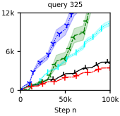
Refer to caption
Refer to caption
Refer to caption
Refer to caption
Refer to caption
Refer to caption
Refer to caption
Refer to caption
Refer to caption
Refer to caption
Refer to caption
Refer to caption
Refer to caption
Refer to caption
Refer to caption
Refer to caption
Refer to caption
Refer to caption
Refer to caption
Refer to caption
Figure 2: The n-step regret of π–’π–Ίπ—Œπ–Όπ–Ίπ–½π–Ύπ–£π–΄π–’π–‘π–’π–Ίπ—Œπ–Όπ–Ίπ–½π–Ύπ–£π–΄π–’π–‘{\sf CascadeDUCB} (black), π–’π–Ίπ—Œπ–Όπ–Ίπ–½π–Ύπ–²π–Άπ–΄π–’π–‘π–’π–Ίπ—Œπ–Όπ–Ίπ–½π–Ύπ–²π–Άπ–΄π–’π–‘{\sf CascadeSWUCB} (red), 𝖱𝖺𝗇𝗄𝖾𝖽𝖀𝖷𝖯πŸ₯𝖱𝖺𝗇𝗄𝖾𝖽𝖀𝖷𝖯πŸ₯\sf RankedEXP3 (cyan), π–’π–Ίπ—Œπ–Όπ–Ίπ–½π–Ύπ–ͺπ–«βˆ’π–΄π–’π–‘π–’π–Ίπ—Œπ–Όπ–Ίπ–½π–Ύπ–ͺ𝖫𝖴𝖒𝖑{\sf CascadeKL\mathchar 45\relax UCB} (green) and π–‘π—Žπ–»π–»π—…π–Ύπ–±π–Ίπ—‡π—„π–‘π—Žπ–»π–»π—…π–Ύπ–±π–Ίπ—‡π—„{\sf BubbleRank} (blue) on single queries in up to 100100100k steps. Lower is better. The results are averaged over 101010 runs per query. The shaded regions represent standard errors of our estimates.