The first eigenvalue and eigenfunction of a nonlinear elliptic system

Abstract.

In this paper, we study the first eigenvalue of a nonlinear elliptic system involving $p$-Laplacian as the differential operator. The principal eigenvalue of the system and the corresponding eigenfunction are investigated both analytically and numerically. An alternative proof to show the simplicity of the first eigenvalue is given. In addition, an upper and lower bounds of the first eigenvalue are provided. Then, a numerical algorithm is developed to approximate the principal eigenvalue. This algorithm generates a decreasing sequence of positive numbers and various examples numerically indicate its convergence. Further, the algorithm is generalized to a class of gradient quasilinear elliptic systems.

Keywords: nonlinear elliptic system, $p$-Laplacian, eigenvalue problem, simplicity, numerical approximation
2010 MSC: 35P30, 34L15, 34L16, 35J92

1. Introduction

Nonlinear elliptic eigenvalue problems form a class of important problems in the theory and applications of partial differential equations and they have been extensively studied in the past decades by many researchers. In particular, problems involving $p$-Laplace operator are of great interest and importance from both the theoretical and applied aspects [1, 18, 19, 20, 21, 23, 24].

In this paper, we consider a nonlinear elliptic system involving two nonlinear eigenvalue problems where the differential operators are two $p$-Laplace operators. The system is weakly coupled such that the two solution components interact through the source terms only.

Let $\Omega\subset\mathbb{R}^{N}$ be a bounded domain with smooth boundary. Our aim is to study, both analytically and numerically, the principal eigenvalue denoted by $\lambda(p,q)$ and the corresponding first eigenfunction $(u,v)$ of the following elliptic eigenvalue system

$$\left\{\begin{array}[]{lrl}-\Delta_{p}u=\lambda|u|^{\alpha-1}|v|^{\beta-1}v&\text{in }\Omega,\\ -\Delta_{q}v=\lambda|u|^{\alpha-1}|v|^{\beta-1}u&\text{in }\Omega,\\ u=v=0&\text{on }\partial\Omega,\end{array}\right.$$ (1.1)

where $\Delta_{p}u=\text{div}(|\nabla u|^{p-2}\nabla u)$ is the $p$-Laplacian and $p,q>1$ and $\alpha,\beta\geq 1$ are real numbers satisfying

$$\frac{\alpha}{p}+\frac{\beta}{q}=1.$$ (1.2)

The first eigenvalue $\lambda(p,q)$ of system (1.1) is defined as the least positive parameter $\lambda$ for which system (1.1) has a solution $(u,v)$ in ${W^{1,p}_{0}(\Omega)\times W^{1,q}_{0}(\Omega)}$ such that both $u\neq 0$ and $v\neq 0$. This eigenvalue problem has a variational form which will be explained in the next section.

The elliptic system (1.1) has been studied in [17] and some close variants of it have been studied in several works, let us mention for example [8, 9, 4, 5, 25]. In particular, these papers investigate the first eigenvalue, the corresponding eigenfunction, their existence, uniqueness, positivity, and isolation in bounded or unbounded domains, with various boundary conditions (see, e.g. [5] and the references therein). The coupled system (1.1) arises in different fields of application. For instance, the case $p>2$ appears in the study of non-Newtonian fluids, pseudoplastics and the case $1<p<2$ in reaction-diffusion problems, flows through porous media, nonlinear elasticity, and glaciology for $p=\frac{4}{3}$, see [17].

In [27] the author studies properties of the positive principal eigenvalue for the following degenerate elliptic system

$$\left\{\begin{array}[]{lrl}-\textrm{div}(\nu_{1}(x)|\nabla u|^{p-2}\nabla u)=\lambda\,a(x)|u|^{p-2}u+\lambda\,b(x)|u|^{\alpha-1}|v|^{\beta-1}v&\text{in }\Omega,\\ -\textrm{div}(\nu_{2}(x)|\nabla v|^{p-2}\nabla v)=\lambda\,d(x)|v|^{q-2}v+\lambda\,b(x)|u|^{\alpha-1}|v|^{\beta-1}u&\text{in }\Omega,\\ u=v=0&\text{on }\partial\Omega,\end{array}\right.$$ (1.3)

where $p,q>1$ and $\alpha,\beta\geq 1$ satisfy (1.2). Note that choosing $\nu_{1}(x)=\nu_{2}(x)=1$, $a(x)=d(x)=0$, and $b(x)=1$ in system (1.3), we obtain system (1.1). The main result [27, Theorem 1.1] applied to this special case provides the simplicity and isolation of the first eigenvalue of (1.1) and positivity of corresponding first eigenfunction. More precisely, it states that the system (1.1) admits a positive principal eigenvalue $\lambda_{1}$, satisfying

$$\lambda_{1}=\underset{(u,v)\in L}{\textrm{inf}}\left[\frac{\alpha}{p}\int_{\Omega}|\nabla u|^{p}\,dx+\frac{\beta}{q}\int_{\Omega}|\nabla v|^{q}\,dx\right],$$

where the set $L$ is

$$L=\left\{(u,v)\in W^{1,p}_{0}(\Omega)\times W^{1,q}_{0}(\Omega):\,\int_{\Omega}|u|^{\alpha}|v|^{\beta}\,dx=1\right\}.$$

Furthermore, each component of the associated normalized eigenfunction $(u_{1},v_{1})$ is nonnegative.

We address some analytical aspects of the first eigenvalue and the corresponding eigenfunction of system (1.1) in this paper. We provide a different proof of the simplicity of $\lambda(p,q)$ which has been first addressed in [17]. Moreover, it is established that system (1.1) reduced to the $p$-Laplacian eigenvalue problem when $p=q$. Next, we will derive a lower and upper estimate for the principal eigenvalue of system (1.1).

Deriving sharp bounds for eigenvalues of elliptic systems is a challenging problem which has been investigated by several authors, e.g. [4, 5, 25].

In general, the value of the first eigenvalue of (1.1) is not explicitly known even for one dimensional problem; but it is important to determine it due to numerous physical applications. However, for the specific case $p=q$, the system is reduced to the scalar $p$-Laplace eigenvalue problem and the spectrum is known exactly in dimension one. To this end, we develop a numerical algorithm computing an approximation of the principal eigenvalue. The algorithm is robust and efficient for various domains with different values of parameters $p,q,\alpha$ and $\beta$. Moreover, we explain how to generalize it for a large class of quasilinear elliptic systems. We prove its convergence in the case $p=q$ where the system reduces to the $p$-Laplace eigenvalue problem.

It is worth to mention that the corresponding scalar equation, i.e., the $p$-Laplace eigenvalue problem, has been studied intensively from both the analytical and numerical point of view [11, 12, 18, 19, 20, 21].

The paper is organized as follows. In section 2, we provide important definitions, recall needed mathematical background and present preliminary results. In section 3, we provide an alternative proof of the simplicity of $\lambda(p,q)$ which has been first addressed in [17]. Further, lower and upper estimates for the principal eigenvalue will be obtained in this section. Section 4 describes the numerical algorithm. In section 5, we provide several numerical examples illustrating the efficiency and applicability of this method.

2. Mathematical Background

In this section we provide the necessary mathematical background. Let us at first address the scalar $p$-Laplace eigenvalue problem.

The first eigenvalue of the $p$-Laplace operator in $W^{1,p}_{0}(\Omega),$ denoted by $\lambda(p)$ for $1\leq p<\infty$ is given by

$$\lambda(p)=\underset{u\neq 0}{\underset{u\in W^{1,p}_{0}(\Omega)}{\min}}\frac{\int_{\Omega}|\nabla u(x)|^{p}dx}{\int_{\Omega}|u(x)|^{p}dx}.$$ (2.1)

The corresponding Euler-Lagrange equation is

$$\text{div}(|\nabla u|^{p-2}\nabla u)+\lambda(p)|u|^{p-2}u=0.$$ (2.2)

Equation (2.2) is interpreted in the usual weak form with test-functions in $W^{1,p}_{0}(\Omega)$:

Definition 2.1.

A nonzero function $u\in W^{1,p}_{0}(\Omega)\cap C(\overline{\Omega}),$ is called a $p$-eigenfunction, if there exists $\lambda(p)\in\mathbb{R}$ such that

$$\int_{\Omega}|\nabla u|^{p-2}\nabla u\cdot\nabla\phi\,dx=\lambda(p)\int_{\Omega}|u|^{p-2}u\,\phi\,dx,\quad\forall\,\phi\in W^{1,p}_{0}(\Omega).$$

The associated number $\lambda(p)$ is called a $p$-eigenvalue. For every $1<p<\infty,$ the first (i.e. the smallest) eigenvalue is simple and isolated and the corresponding eigenfunction is a bounded continuous function on $\overline{\Omega}$ which does not change sign [19].

There are two important limit cases; as $p$ tends to one and infinity. We recall the result of [15], which says that the first eigenvalue $\lambda(p)$ converges to the Cheeger constant $h(\Omega)$ as $p\rightarrow 1$. Furthermore, the associated eigenfunction converges to the characteristic function $\chi_{C_{\Omega}}$ of the Cheeger set $C_{\Omega}$, i.e., the subset of $\Omega$ which minimizes the ratio $|\partial D|/|D|$ among all simply connected $D\subset\Omega$.

The first eigenvalue $\Lambda_{\infty}$ of the infinity Laplacian corresponds to the reciprocal value of the radius of the largest ball that can be inscribed in the domain $\Omega$. More precisely

$$\Lambda_{\infty}=\frac{1}{\underset{x\in\Omega}{\max}\,\text{dist}(x,\partial\Omega)}=\underset{p\rightarrow\infty}{\lim}\lambda(p)^{\frac{1}{p}},$$

where $\lambda(p)$ is the first eigenvalue of the $p$-Laplace operator, see [19]. In addition, if the domain is a ball, then the infinity eigenfunction is the distance function $d(x)=\text{dist}(x,\partial\Omega)$. Obviously, for a unite ball centered at the origin $d(x)=1-|x|$ and $\Lambda_{\infty}=1$.

Now, we return to the nonlinear system (1.1).

Definition 2.2.

The first eigenvalue $\lambda(p,q)$ of (1.1) is defined as the least positive parameter $\lambda$ for which system (1.1) has a solution $(u,v)$ in the product Sobolev space $W^{1,p}_{0}(\Omega)\times W^{1,q}_{0}(\Omega)$ such that both $u\neq 0$ and $v\neq 0$.

Here by a solution to (1.1) we mean a pair $(u,v)$ in $W^{1,p}_{0}(\Omega)\times W^{1,q}_{0}(\Omega)$ such that

$$\int_{\Omega}|\nabla u|^{p-2}\nabla u\cdot\nabla\phi\,dx+\int_{\Omega}|\nabla v|^{q-2}\nabla u\cdot\nabla\psi\,dx=$$

$$\lambda\left(\int_{\Omega}|u|^{\alpha-1}|v|^{\beta-1}v\phi\,dx+\int_{\Omega}|u|^{\alpha-1}|v|^{\beta-1}u\psi\,dx\right),$$ (2.3)

$$\quad\forall\,(\phi,\psi)\in W^{1,p}_{0}(\Omega)\times W^{1,q}_{0}(\Omega).$$

Defining the Rayleigh quotient

$$\mathcal{R}(u,v)=\frac{\frac{\alpha}{p}\int_{\Omega}|\nabla u(x)|^{p}dx+\frac{\beta}{q}\int_{\Omega}|\nabla v(x)|^{q}dx,}{\int_{\Omega}|u(x)|^{\alpha-1}|v(x)|^{\beta-1}u(x)v(x)dx},$$

the principal eigenvalue $\lambda(p,q)$ can be variationally characterized by minimizing the functional $\mathcal{R}$ over the set

$$\mathcal{A}=\left\{(u,v)\in W^{1,p}_{0}(\Omega)\times W^{1,q}_{0}(\Omega):\int_{\Omega}|u(x)|^{\alpha-1}|v(x)|^{\beta-1}u(x)v(x)dx>0\right\}.$$

Thus

$$\lambda(p,q)=\min\left\{\mathcal{R}(u,v),(u,v)\in\mathcal{A}\right\}$$ (2.4)

and the minimizer is the pair of eigenfunctions $(u,v)$, see [17]. If $(u,v)$ is the pair of eigenfunctions corresponding to the first eigenvalue of (1.1), then

$$\mathcal{R}(|u|,|v|)\leq\mathcal{R}(u,v),$$

because

$$\int_{\Omega}|u|^{\alpha-1}|v|^{\beta-1}uvdx\leq\int_{\Omega}|u|^{\alpha-1}|v|^{\beta-1}|u||v|dx.$$

Consequently, in view of variational formulation (2.4), we deduce that if $(u,v)$ is a minimizer in (2.4), so is $(|u|,|v|)$. Therefore we may assume that $u$ and $v$ are nonnegative. In addition, if the pair $(u,v)$ is a nonnegative weak solution to (1.1), then $u,v>0$ in $\Omega$ due to the maximum principle of Vàzquez [26]. As mentioned in introduction, to see about simplicity of first eigenvalue and positivity of corresponding eigenfunction for general system (1.3) we refer to [27].

The existence of a principal eigenvalue, simplicity and the isolation of the first eigenvalue have been proved for (1.1) and its variants in [4, 5, 17, 10, 25]. Let us recall that the first eigenvalue $\lambda(p,q)$ of (1.1) is simple if for any two pairs of corresponding eigenfunctions $(u,v)$ and $(\phi,\psi)$ there exist real numbers $k_{1}$ and $k_{2}$ such that $u=k_{1}\phi$ and $v=k_{2}\psi$.

3. Analytical results

In this section we examine certain analytical aspects of system (1.1). Simplicity of the principal eigenvalue is one of its main features and it has been investigated in [17]. Here we provide an alternative proof which is more straightforward and based on the proof given by Belloni and Kahwol [3] establishing the simplicity of the principal eigenvalue of scalar problem (2.2).

Theorem 3.1.

The first eigenvalue of system (1.1) is simple.

Proof.

Let $(u,v)$ and $(\phi,\psi)$ be two pairs of eigenfunctions associate with $\lambda(p,q)$. As we mentioned above, we assume that $u,v>0$ and $\phi,\psi>0$ in $\Omega$. Without loss of generality, we assume that these eigenfunctions are normalized such that

$$\int_{\Omega}u^{\alpha}\,v^{\beta}\,dx=\int_{\Omega}\phi^{\alpha}\,\psi^{\beta}\,dx=1.$$

We show that there exist real numbers $k_{1},k_{2}$ such that $u=k_{1}\phi$ and $v=k_{2}\psi$. Note that

$$w_{1}=\left(\frac{u^{p}+\phi^{p}}{2}\right)^{\frac{1}{p}}\quad\text{and}\quad w_{2}=\left(\frac{v^{q}+\psi^{q}}{2}\right)^{\frac{1}{q}}$$

are admissible functions which means they belong to $\mathcal{A}$. In view of variational form (2.4), we observe that

$$\lambda(p,q)\leq\frac{\frac{\alpha}{p}\int_{\Omega}|\nabla w_{1}|^{p}dx+\frac{\beta}{q}\int_{\Omega}|\nabla w_{2}|^{q}dx}{\int_{\Omega}w_{1}^{\alpha}w_{2}^{\beta}\,dx}.$$ (3.1)

We show that

$$w_{1}^{\alpha}w_{2}^{\beta}=\left(\frac{u^{p}+\phi^{p}}{2}\right)^{\frac{\alpha}{p}}\,\left(\frac{v^{q}+\psi^{q}}{2}\right)^{\frac{\beta}{q}}\geq\frac{1}{2}(u^{\alpha}v^{\beta}+\phi^{\alpha}\psi^{\beta}).$$ (3.2)

Due to the Hölder’s inequality for counting measure, we observe that

$$(u^{\alpha},\phi^{\alpha})\cdot(v^{\beta},\psi^{\beta})\leq\left(u^{\frac{\alpha p}{\alpha}}+\phi^{\frac{\alpha p}{\alpha}}\right)^{\frac{\alpha}{p}}\left(v^{\frac{\beta q}{\beta}}+\psi^{\frac{\beta q}{\beta}}\right)^{\frac{\beta}{q}},$$

which yields (3.2). Thus, (3.1) and (3.2), and the normalization of $(u,v)$ and $(\phi,\psi)$ yields

$$\lambda(p,q)\leq\frac{\alpha}{p}\int_{\Omega}|\nabla w_{1}|^{p}\,dx+\frac{\beta}{q}\int_{\Omega}|\nabla w_{2}|^{q}\,dx.$$ (3.3)

For gradients of $w_{1}$ and $w_{2}$ we have

$$|\nabla w_{1}|^{p}=\left(\frac{u^{p}+\phi^{p}}{2}\right)\left|\frac{u^{p}\nabla\log\,u+\phi^{p}\nabla\log\,\phi}{u^{p}+\phi^{p}}\right|^{p},$$

$$|\nabla w_{2}|^{q}=\left(\frac{v^{q}+\psi^{q}}{2}\right)\left|\frac{v^{q}\nabla\log\,v+\psi^{q}\nabla\log\,\psi}{v^{q}+\psi^{q}}\right|^{q}.$$

Recalling Jensen’s inequality

$$\theta\left(\frac{\Sigma a_{i}x_{i}}{\Sigma a_{i}}\right)\leq\frac{\Sigma a_{i}\theta(x_{i})}{\Sigma a_{i}}$$

for convex function $\theta(\cdot)=|\cdot|^{p}$, we obtain by choosing

$$\left\{\begin{array}[]{ll}a_{1}=\frac{u^{p}}{u^{p}+\phi^{p}},\quad a_{2}=\frac{\phi^{p}}{u^{p}+\phi^{p}},\\ x_{1}=\nabla\log\,u,\quad x_{2}=\nabla\log\,\phi,\end{array}\right.$$

the following inequalities:

$$|\nabla w_{1}|^{p}\leq\frac{1}{2}|\nabla u|^{p}+\frac{1}{2}|\nabla\phi|^{p},$$

$$|\nabla w_{2}|^{q}\leq\frac{1}{2}|\nabla v|^{q}+\frac{1}{2}|\nabla\psi|^{q}.$$

These inequalities are strict at points where

$$\nabla\log u(x)\neq\nabla\log\phi(x)\quad\text{and}\quad\nabla\log\,v(x)\neq\nabla\log\,\psi(x).$$

Therefore, we assume for the moment that $\nabla\log\,u\neq\nabla\log\,\phi$ or $\nabla\log\,v\neq\nabla\log\,\psi$ in a set of positive measure. Consequently, inequality (3.3) implies

$$\lambda(p,q)<\frac{\alpha}{2p}\int_{\Omega}(|\nabla u|^{p}+|\nabla\phi|^{p})\,dx+\frac{\beta}{2q}\int_{\Omega}(|\nabla v|^{q}+|\nabla\psi|^{q})\,dx=\lambda(p,q),$$ (3.4)

where the last equality follows from (2.4) and the fact that $(u,v)$ and $(\phi,\psi)$ are normalized. Contradiction (3.4) shows that

$$\nabla\log u=\nabla\log\,\phi\quad\text{and}\quad\nabla\log v=\nabla\log\psi\quad\text{a.e. in}\quad\Omega.$$

Therefore there exist constants $k_{1}$ and $k_{2}$ such that $u=k_{1}\phi$ and $v=k_{2}\psi$.

∎

One interesting feature of system (1.1) is that it will reduce to the scalar equation (2.2) with Dirichlet boundary conditions for $p=q$.

Theorem 3.2.

Let $p=q$ and $(u,v)$ be a solution of (1.1). Then $u$ equals $v$ in $\Omega$ for all $\alpha,\beta\geq 1$ satisfying (1.2). Moreover, function $u=v$ solves (2.2).

Proof.

Suppose that $u\neq v$ in $\Omega$. Then, without loss of generality, there is a subset $D$ of $\Omega$ of positive measure such that

$$D=\{x\in\Omega:u(x)<v(x)\}.$$

The set $D$ is an open set due to the fact that $u,v\in C^{1}({\Omega})$, see [17]. We define

$$\eta(x)=\left\{\begin{array}[]{ll}v(x)-u(x)&\text{in }D,\\ 0&\text{in }\Omega\setminus D.\end{array}\right.$$

This $\eta$ belongs to $W^{1,p}(\Omega)$. Considering $\eta$ as a test function, variational formulation (2) with $p=q$ and $\lambda=\lambda(p,q)$ yields

$$\int_{D}|\nabla u|^{p-2}\nabla u\cdot\nabla\eta\,dx=\lambda\int_{D}u^{\alpha-1}v^{\beta}\eta dx,$$

$$\int_{D}|\nabla v|^{p-2}\nabla v\cdot\nabla\eta\,dx=\lambda\int_{D}u^{\alpha}v^{\beta-1}\eta dx,$$

and consequently, we have

$$\int_{D}(|\nabla v|^{p-2}\nabla v-|\nabla u|^{p-2}\nabla u)\cdot\nabla(u-v)\,dx=\lambda\int_{D}u^{\alpha-1}v^{\beta-1}(u-v)(v-u)\,dx.$$ (3.5)

In view of the positivity of the eigenfunctions of (1.1), the right hand side of (3.5) is negative. Recalling the inequality from [21]:

$$\left<|b|^{p-2}b-|a|^{p-2}a,b-a\right>>0,\>\;\forall a,b\in\mathbb{R}^{N},\,a\neq b,\>\;\text{and}\>\;p>1,$$

where $\left<\cdot,\cdot\right>$ denotes the inner product in $\mathbb{R}^{N}$ and setting $b=\nabla v$ and $a=\nabla u$, we deduce that the left hand side of (3.5) is a positive quantity. This is a contradiction with the negativity of the right hand side and, thus, $u=v$ in $\Omega$. ∎

Now, we will provide some upper and lower bounds for the first eigenvalue of system (1.1). Such estimates for eigenvalues have been considered for similar systems in various papers, for example [4, 5, 25]. First, we prove the lower bound.

Theorem 3.3.

Let $\lambda(p,q)$ be defined by (2.4), then

$$\lambda(p,q)\geq\min\{\lambda(p),\lambda(q)\},$$

where $\lambda(p)$ and $\lambda(q)$ are the principal eigenvalues of $p$-Laplacian given by (2.1).

Proof.

Let $(u,v)$ be the normalized eigenfunction associated with $\lambda(p,q)$. Using Young’s inequality, we obtain

$$\lambda(p,q)=\frac{\frac{\alpha}{p}\int_{\Omega}|\nabla u|^{p}dx+\frac{\beta}{q}\int_{\Omega}|\nabla v|^{q}dx}{\int_{\Omega}u^{\alpha}v^{\beta}\,dx}\geq\frac{\frac{\alpha}{p}\int_{\Omega}|\nabla u|^{p}dx+\frac{\beta}{q}\int_{\Omega}|\nabla v|^{q}dx}{\frac{\alpha}{p}\int_{\Omega}u^{p}dx+\frac{\beta}{q}\int_{\Omega}v^{q}dx}.$$

Applying inequality

$$\frac{a+b}{c+d}\geq\min\left\{\frac{a}{c},\frac{b}{d}\right\}$$

with $a=\frac{\alpha}{p}\int_{\Omega}|\nabla u|^{p}dx$, $b=\frac{\beta}{q}\int_{\Omega}|\nabla v|^{q}dx$, etc., we obtain

$$\lambda(p,q)\geq\min\left\{\frac{\int_{\Omega}|\nabla u|^{p}dx}{\int_{\Omega}u^{p}dx},\>\frac{\int_{\Omega}|\nabla v|^{q}dx}{\int_{\Omega}v^{q}dx}\right\}\geq\min\{\lambda(p),\lambda(q)\}.$$

∎

Determining an upper bound for the first eigenvalue is a more subtle problem and we will investigate it for certain special cases. First, we address this question in dimension $N=1$. The upper bound derived below is based on the following theorem from [7].

Theorem 3.4.

Let $a_{1},\dots,a_{n}$ be real numbers all greater or equal to 1. Suppose that

$$\min_{{I\subseteq\{1,\dots,n\}}}\left|\sum_{k\in I}a_{k}-\frac{1}{2}\sum_{k=1}^{n}a_{k}\right|,$$

is attained for $I=I_{0}$. Set

$$a_{0}=\underset{k\in I_{0}}{\sum}a_{k},\qquad a_{00}=\underset{k\notin I_{0}}{\sum}a_{k}.$$

Let $g_{1},\dots,g_{n}$ be nonnegative functions on the interval $(0,1)$ such that the function $g_{1}^{1/a_{1}},\dots,g_{n}^{1/a_{n}}$ are concave and let $p_{1},\dots,p_{n}$ be real numbers greater or equal to 1. Then

$$\int_{0}^{1}\prod_{k=1}^{n}g_{k}(x)dx\geq C\prod_{k=1}^{n}\left(\int_{0}^{1}g_{k}^{p_{k}}(x)dx\right)^{1/p_{k}},$$

where

$$C=\left(\prod_{k=1}^{n}(1+a_{k}p_{k})^{1/p_{k}}\right)\mathcal{B}(1+a_{0},1+a_{00}),$$

and $\mathcal{B}$ stands for the beta function

$$\mathcal{B}(r,s)=\int_{0}^{1}x^{r-1}(1-x)^{s-1}dx.$$

Now we are prepared to prove the following theorem.

Theorem 3.5.

Let $\Omega=(0,1)$ then for the principal eigenvalue of (1.1) we have

$$\lambda(p,q)\leq\frac{1}{C}\left(\frac{\alpha}{p}\lambda(p)+\frac{\beta}{q}\lambda(q)\right),$$ (3.6)

where

$$C=(1+p)^{\alpha/p}(1+q)^{\beta/q}\mathcal{B}(1+\alpha,1+\beta).$$

Proof.

Let $u=u(p)$ and $v=u(q)$ be the eigenfunctions associate with $\lambda(p)$ and $\lambda(q)$ respectively and let they be normalized such that $\|u\|_{L^{p}(\Omega)}=\|v\|_{L^{q}(\Omega)}=1.$ In Theorem 3.4, we set

$$a_{1}=\alpha,\;a_{2}=\beta,\;g_{1}=u^{\alpha},\;g_{2}=v^{\beta},\;p_{1}=\frac{p}{\alpha},\;p_{2}=\frac{q}{\beta}.$$

From here

$$a_{0}=\alpha,\;a_{00}=\beta.$$

Recall that $\alpha,\beta\geq 1$ and also $\frac{p}{\alpha},\frac{q}{\beta}\geq 1$ regarding the fact that $\frac{\alpha}{p}+\frac{\beta}{q}=1$. It is known that the first eigenfunction of (2.2) is concave for one dimensional problems [19]. Hence, functions $g_{1},g_{2}$ are concave as well. Thus, in view of Theorem 3.4 we observe that

$$\int_{0}^{1}g_{1}g_{2}dx=\int_{0}^{1}u^{\alpha}v^{\beta}dx\geq C\|u\|_{L^{p}(\Omega)}^{\alpha}\|v\|_{L^{q}(\Omega)}^{\beta}=C,$$ (3.7)

where

$$C=(1+p)^{\alpha/p}(1+q)^{\beta/q}\mathcal{B}(1+\alpha,1+\beta).$$

Applying the variational characterization (2.4), we infer that

$$\lambda(p,q)\leq\frac{\frac{\alpha}{p}\int_{\Omega}|\nabla u(x)|^{p}dx+\frac{\beta}{q}\int_{\Omega}|\nabla v(x)|^{q}dx,}{\int_{\Omega}u^{\alpha}v^{\beta}dx}=\frac{\frac{\alpha}{p}\lambda(p)+\frac{\beta}{q}\lambda(q)}{\int_{0}^{1}u^{\alpha}v^{\beta}dx},$$

and then employing (3.7) we obtain (3.6).

∎

The above proof is strongly based upon the concavity of the first eigenfunctions of (2.2) in dimension one. It is worth noting that the first eigenfunction of (2.2) is not concave, in higher dimensions in general [19]. Note that another upper bound for dimension one is given in [6, Section 5].

Concerning two dimensions, we obtain an upper bound for the first eigenvalue when $\alpha=\beta=1$, provided the following hypothesis holds true.

Hypothesis 1.

If $u(p)$ denotes the eigenfunction corresponding to the first eigenvalue of the scalar $p$-Laplacian (2.2) normalized such that $\|u(p)\|_{L^{p}(\Omega)}=1$ then

$$\int_{\Omega}u(p)u(q)\,dx\geq\int_{\Omega}u(1)u(\infty)\,dx$$ (3.8)

for all $p,q\in[1,\infty]$ satisfying $1/p+1/q=1$.

This hypothesis can be investigated by introducing function

$$f(p)=\int_{\Omega}u(p)u\left(\frac{p}{p-1}\right)\,dx\quad\text{for }p\in[1,\infty],$$ (3.9)

where the value of $p/(p-1)$ for $p=1$ and $p=\infty$ is understand to be $\infty$ and $1$, respectively. Note that function $f(p)$ is symmetric in the sense

$$f(p)=f\left(\frac{p}{p-1}\right)\quad\text{for all }p\in[1,\infty].$$

Consequently, it is sufficient to investigate $f(p)$ for $p\in[2,\infty]$ only. Hypothesis (3.8) is equivalent to the statement $f(p)\geq f(\infty)$ for all $p\in[2,\infty]$.

It is easy to show that the maximum of $f$ is attained at 2. Indeed,

$$f(p)=\int_{\Omega}u(p)u(q)\leq\|u(p)\|_{L^{p}(\Omega)}\|u(q)\|_{L^{q}(\Omega)}=1\quad\text{and}\quad f(2)=\|u(2)\|_{L^{2}(\Omega)}^{2}=1.$$

Thus, if $f(p)$ were nonincreasing for $p\in[2,\infty]$ then the minimum of $f(p)$ would be attained at $p=\infty$ and Hypothesis 1 would hold true. However, the monotonicity of $f(p)$ is not clear.

One possibility how to investigate it is to show the existence and nonnegativity of the derivative

$$f^{\prime}(p)=\frac{-1}{(p-1)^{2}}f^{\prime}\left(\frac{p}{p-1}\right)$$

for $p\in[2,\infty]$. Figure 1 shows numerically computed values of $f(p)$ for interval $\Omega=(0,1)$. These results indicate that $f(p)$ is smooth, its derivative is positive in $[1,2]$, negative in $[2,\infty]$, $f^{\prime}(2)=0$, and consequently that Hypothesis 1 holds true. Note that in this case $u(1)=\chi_{\Omega}$ is the characteristic function of $\Omega$, $u(\infty)=1-|2x-1|$ is the distance function, and hence $f(1)=f(\infty)=1/2$.

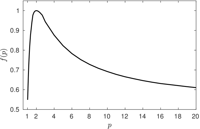
Figure 1. The graph of function $f(p)$ defined in (3.9) for $\Omega=(0,1)$.

Theorem 3.6.

Assume Hypothesis 1 holds true. Let $\Omega$ be a convex subset of $\mathbb{R}^{2}$ and let $\alpha=\beta=1$. Then for the principal eigenvalue of (1.1) we have

$$\lambda(p,q)\leq\frac{3\,|\Omega|}{|B_{\varrho}|}\left(\frac{1}{p}\lambda(p)+\frac{1}{q}\lambda(q)\right),$$ (3.10)

where $B_{\varrho}$ denotes the largest disc that can be inscribed in $\Omega$ and $\lambda(p),\lambda(q)$ are the principal eigenvalues given by (2.1) and corresponding to $p,q$, respectively.

Proof.

Considering eigenfunctions $u=u(p)$ and $v=u(q)$ as in the proof of Theorem 3.5 and using the variational characterization (2.4), we observe that

$$\lambda(p,q)\leq\frac{\frac{1}{p}\int_{\Omega}|\nabla u(x)|^{p}dx+\frac{1}{q}\int_{\Omega}|\nabla v(x)|^{q}dx,}{\int_{\Omega}uvdx}=\frac{\frac{1}{p}\lambda(p)+\frac{1}{q}\lambda(q)}{\int_{\Omega}uvdx},$$

The need lower bound for $\int_{\Omega}uv\,dx$ is provided by Hypothesis 1:

$$\int_{\Omega}u(1)u(\infty)\,dx\leq\int_{\Omega}uv\,dx,$$

where $u(1)$ and $u(\infty)$ are normalized in $L^{1}(\Omega)$ and $L^{\infty}(\Omega)$, respectively. We know that

$$\int_{\Omega}u(1)u(\infty)\,dx=\frac{1}{|C_{\Omega}|}\int_{\Omega}\chi_{C_{\Omega}}\,u(\infty)\,dx=\frac{1}{|C_{\Omega}|}\int_{C_{\Omega}}u(\infty)\,dx.$$

Further, let $B_{\varrho}$ be a largest disc inscribed to $\Omega$ and let $\varrho$ be its radius. The normalized eigenfunction of the $\infty$-Laplacian in the disc $B_{\varrho}$ is $d_{B}/\varrho$, where

$$d_{B}(x)=\text{dist}(x,\partial B_{\varrho}).$$

If we extend $d_{B}$ by zero then

$$u(\infty)\geq\frac{1}{\varrho}d_{B}\quad\text{in }\Omega,$$

because $B_{\varrho}\subset\Omega$. Thus,

$$\frac{1}{|C_{\Omega}|}\int_{C_{\Omega}}u(\infty)\,dx\geq\frac{1}{\varrho\,|C_{\Omega}|}\int_{C_{\Omega}}d_{B}(x)\,dx\geq\frac{1}{\varrho\,|C_{\Omega}|}\int_{B_{\varrho}}d_{B}(x)\,dx=\frac{|B_{\varrho}|}{3\,|C_{\Omega}|}\geq\frac{|B_{\varrho}|}{3\,|\Omega|},$$

where we use the fact that $B_{\varrho}\subset C_{\Omega}$. This inclusion follows from [16, Theorem 1], where the convexity of $\Omega$ is assumed. This theorem states that there exists $t^{*}>0$ such that $C_{\Omega}=\Omega^{t^{*}}+t^{*}B_{1}$, where $\Omega^{t^{*}}=\{x\in\Omega:\operatorname{dist}(x,\partial\Omega)>t^{*}\}$, $B_{1}$ is the unit disc and the addition is the Minkowski addition of sets, i.e., $A+B=\{a+b:a\in A,\ b\in B\}$. Shifting $\Omega$ such that the center of $B_{\varrho}$ is at origin, we immediately see that $(\varrho-t^{*})B_{1}\subset\Omega^{t^{*}}$. Consequently, $C_{\Omega}\supset(\varrho-t^{*})B_{1}+t^{*}B_{1}=B_{\varrho}$.

To conclude, we obtained

$$\int_{\Omega}uvdx\geq\frac{|B_{\varrho}|}{3\,|\Omega|}$$

and the proof is finished. ∎

Remark 3.1.

If the domain is a ball in $\mathbb{R}^{N}$ or a domain where the first eigenfunction of the infinity Laplace operator is the distance function, then it is easy to see that

$$\int_{\Omega}u(1)v(\infty)\,dx=\frac{1}{N+1}.$$

This yields (under Hypothesis 1) upper bound

$$\lambda(p,q)\leq(N+1)\left(\frac{1}{p}\lambda(p)+\frac{1}{q}\lambda(q)\right).$$

Interestingly, estimate (3.10) turns to this bound if $\Omega$ is chosen as a disc in Theorem 3.6.

4. An algorithm to approximate the first eigenvalue and the first eigenfunction

Algorithm 1 computes an approximation of the first eigenvalue and the corresponding eigenfunction of (1.1).


Algorithm 1 (1) Set $k=0$ and choose an initial guess $(u,v)\in W^{1,p}_{0}(\Omega)\times W^{1,q}_{0}(\Omega)$ such that $u,v\geq 0$. (2) Given $u$, $v$, normalize them as $$u_{k}=\frac{u}{(\int_{\Omega}u^{\alpha}v^{\beta}dx)^{\frac{1}{p}}},\quad v_{k}=\frac{v}{(\int_{\Omega}u^{\alpha}v^{\beta}dx)^{\frac{1}{q}}},$$ and calculate $$\lambda^{k}=\frac{\alpha}{p}\int_{\Omega}|\nabla u_{k}|^{p}dx+\frac{\beta}{q}\int_{\Omega}|\nabla v_{k}|^{q}dx.$$ (3) If $k\geq 1$ and $|\lambda^{k}-\lambda^{k-1}|<\varepsilon$, then stop. (4) Otherwise, solve the following decoupled systems: $\displaystyle-\Delta_{p}u$ $\displaystyle=\lambda^{k}u_{k}^{\alpha-1}v_{k}^{\beta}$ $\displaystyle\text{in }\Omega,$ $\displaystyle-\Delta_{q}v$ $\displaystyle=\lambda^{k}u_{k}^{\alpha}v_{k}^{\beta-1}$ $\displaystyle\text{in }\Omega,$ (4.1) $\displaystyle u$ $\displaystyle=v=0$ $\displaystyle\text{on }\partial\Omega,$ set $k=k+1$, and go to the step (2).

Algorithm 1 computes in every iteration an approximation $\lambda^{k}$ of the principal eigenvalue $\lambda(p,q)$ of (1.1). The computed pair of functions $(u_{k},v_{k})$ approximates the corresponding pair of eigenfunctions. Note that functions $(u_{k},v_{k})$ are normalized in every iteration such that $\int_{\Omega}u_{k}^{\alpha}v_{k}^{\beta}dx=1$. The algorithm stops, when the distance between two successive approximate eigenvalues is less than a given tolerance $\varepsilon.$

Remark 1.

In view of Theorem 3.2, we know that (1.1) is reduced to scalar equation (2.2) with Dirichlet boundary conditions when $p=q$. Algorithm 1 in this case reduces to the algorithm developed by the first author in [11] where the convergence of the iterative scheme to the first eigenfunction and the related eigenvalue has been shown.

Remark 2.

In [14] two methods for approximate minimizers of the abstract Rayleigh quotient $\frac{\Phi(u)}{\|u\|^{p}}$ have been presented. The functional $\Phi$ is assumed there to be strictly convex on a Banach space with norm $\|\cdot\|$ and positively homogeneous of degree $p\in(0,\infty)$. These methods, however, are not applicable to calculate the principal eigenvalue of (1.1) since $\mathcal{R}(t^{1/p}u,t^{1/q}v)=\mathcal{R}(u,v).$

Now we discuss the interesting possibility of extending Algorithm 1 to a class of quasilinear elliptic systems called gradient systems. These systems have been studied widely in the past decade, see [2] and the reference therein. Gradient systems are of the following general form:

$$\left\{\begin{array}[]{lrl}-\Delta_{p}u=\lambda F_{u}(x,u,v)&\text{in }\Omega,\\ -\Delta_{q}v=\lambda F_{v}(x,u,v)&\text{in }\Omega,\\ u=v=0&\text{on }\partial\Omega,\\ \end{array}\right.$$ (4.2)

where $1<p,q<\infty$ and $F_{u},\>F_{v}$ denotes partial derivatives. The nonlinearity $F:\Omega\times\mathbb{R}\times\mathbb{R}\rightarrow\mathbb{R}$ is a $C^{1}$- function, satisfying $F(x,0,0)=0$ and

• $F(x,t,s)=F(x,0,s),\quad\forall\>x\in\Omega,\quad s\in\mathbb{R}\quad\text{and}\quad t\leq 0,$

• $F(x,t,s)=F(x,t,0),\quad\forall\>x\in\Omega,\quad t\in\mathbb{R}\quad\text{and}\quad s\leq 0,$

• $\left|F_{t}(x,t,s)\right|\leq c\left(1+|t|^{p-1}+|s|^{q\frac{p-1}{p}}\right),$

• $\left|F_{s}(x,t,s)\right|\leq c\left(1+|s|^{q-1}+|t|^{p\frac{q-1}{q}}\right)$

for all $(x,s,t)\in\Omega\times\mathbb{R}\times\mathbb{R}$. Under these growth conditions on $F$, the principal eigenvalue is the minimum value of the following Rayleigh quotient

$$\mathcal{R}(u,v)=\frac{\frac{1}{p}\int_{\Omega}|\nabla u(x)|^{p}dx+\frac{1}{q}\int_{\Omega}|\nabla v(x)|^{q}dx}{\int_{\Omega}F(x,u(x),v(x))dx},$$

over the set

$$\mathcal{A}={\{(u,v)\in W^{1,p}_{0}(\Omega)\times W^{1,q}_{0}(\Omega):\int_{\Omega}F(x,u(x),v(x))\,dx{>}0}\}.$$

Now, Algorithm 1 can be easily modified to compute the principal eigenvalue of (4.2). To this aim, we just replace decoupled system (4) by decoupled system

$$\left\{\begin{array}[]{lrl}-\Delta_{p}u=\lambda^{k}F_{u}(x,u_{k},v_{k})&\text{in }\Omega,\\ -\Delta_{q}v=\lambda^{k}F_{v}(x,u_{k},v_{k})&\text{in }\Omega,\\ u=v=0&\text{on }\partial\Omega,\end{array}\right.$$ (4.3)

and normalize its solution as

$$u_{k+1}=\frac{u}{\left(\int_{\Omega}F(x,u(x),v(x))\,dx\right)^{\frac{1}{p}}},$$

$$v_{k+1}=\frac{v}{\left(\int_{\Omega}F(x,u(x),v(x))\,dx\right)^{\frac{1}{q}}}.$$

Performed numerical tests indicate that the extended algorithm is convergent and efficiently approximates the principal eigenvalue.

5. Numerical implementation

This section provides several examples in order to illustrate the efficiency of Algorithm 1. At iteration $k$ we solve decoupled nonlinear elliptic system (4) by the finite element method with piecewise linear basis functions. The resulting discrete system of nonlinear equations is solved by a modified Newton-Raphson method. Using a tolerance on the level of the machine precision and a suitable initial approximation, the Newton-Raphson method converges in at most $50$ iterations for all examples below. Similarly, the tolerance in the fourth step of Algorithm 1 was chosen as $\varepsilon=5\times 10^{-5}$ and in all the following examples the algorithm converges in less than 10 iterations.

Example 5.1.

Let $\Omega$ be the unit disc centred at origin. The radial symmetry then enables us to use polar coordinates $u=u(r),\>v=v(r)$, $0<r<1$ and to transform system (1.1) to one dimensional system

$$\left\{\begin{array}[]{lrl}-(r|u^{\prime}|^{p-2}u^{\prime})^{\prime}=\lambda r|u|^{\alpha-1}|v|^{\beta-1}v&\text{in }(0,1),\\ -(r|v^{\prime}|^{q-2}v^{\prime})^{\prime}=\lambda r|u|^{\alpha-1}|v|^{\beta-1}u&\text{in }(0,1),\\ u^{\prime}(0)=v^{\prime}(0)=0\quad u(1)=v(1)=0.\end{array}\right.$$ (5.1)

Note that all finite element computations in the interval $(0,1)$ are performed with 500 elements (subintervals) of the same length.

Let us start with a simple test case $p=q=2$. For this choice and arbitrary values of $\alpha$ and $\beta$ satisfying (1.2), system (1.1) reduces to a scalar eigenvalue problem for the standard Laplace operator. The principal eigenvalue of Laplacian in the unit disc with zero Dirichlet boundary conditions is the square of the first zero of the Bessel function $J_{0}$, i.e., $\lambda_{1}\approx 5.7832$. The sequence $\{\lambda^{k}\}$ computed by Algorithm 1 applied to system (5.1) converges to this value and Table 1 illustrates the speed of this convergence for initial guess $u_{0}=v_{0}=(1-r)^{2}$ and parameter values $\alpha=1$ and $\beta=1$.

Similarly, both sequences $\{u^{k}\}$ and $\{v^{k}\}$ computed by Algorithm 1 converge to the normalized first eigenfunction of the Laplacian

$$w_{1}(r)=J_{0}\left(\lambda_{1}^{1/2}r\right)/\left\|J_{0}\left(\lambda_{1}^{1/2}r\right)\right\|_{L^{2}(\Omega)}.$$

Table 1 shows the speed of this convergence and indicates that it is uniform.

Table 1. The convergence to the principal eigenvalue $\lambda_{1}\approx 5.78318$ and to the corresponding eigenfunction $w_{1}$ computed by Algorithm 1 for the unit disc with $p=q=2$, $\alpha=1$ and $\beta=1$.

$k$	$\lambda^{k}$	$|\lambda_{1}-\lambda^{k}|/\lambda_{1}$	$\|u_{k}-w_{1}\|_{L^{\infty}(\Omega)}$
0	10.0000	0.7291	1.0764
1	5.9232	0.0242	0.1405
2	5.7882	0.0008	0.0246
3	5.7834	0.0000	0.0045
4	5.7832	0.0000	0.0005
5	5.7832	0.0000	0.0001

As a second test, we choose $p=q$ and consider large values of $p$. In this case system (1.1) reduces to the scalar equation (2.2) and it is known [19, Lemma 11] that $\lambda(p)^{1/p}$ converges to $\Lambda_{\infty}=1$ when $p\rightarrow\infty$. We verify this fact numerically by applying Algorithm 1 to system (5.1) with $u_{0}=\cos(\pi r/2),v_{0}=\sin(\pi(r+1)/2)$.

The results are reported in Table 2 and confirm the expectations although the convergence is not as fast as in the previous test. Similarly, the corresponding eigenfunctions are known to converge to the distance function $d(x)=\operatorname{dist}(x,\partial\Omega)$. Figure 2 shows the eigenfunctions computed by Algorithm 1 for three different values of $p$ and confirms the expected convergence.

Table 2. The principal eigenvalue $\lambda(p)$ of $p$-Laplacian in the unit circle computed by Algorithm 1 applied to system (5.1) with $p=q$.

$p$	$\lambda(p)$	$\lambda(p)^{1/p}$	$\|u(x)-d(x)\|_{L^{\infty}(\Omega)}$
1.3	3.2660	2.5205	0.3864
6	26.832	1.7301	0.4316
18	166.02	1.3284	0.2605
30	415.90	1.2226	0.1864
100	4026.9	1.0865	0.0772
200	15498	1.0494	0.0449
300	34363	1.0354	0.0325
400	60610	1.0279	0.0257

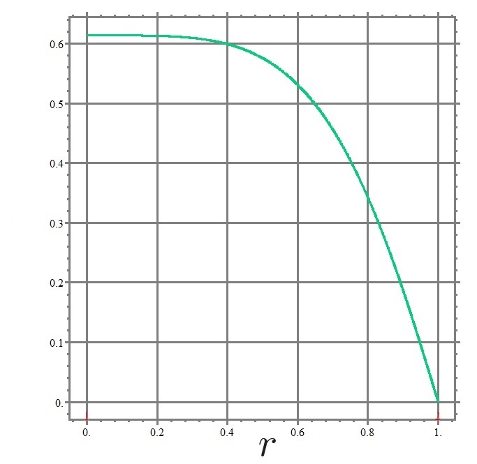
(a) $p=1.3$

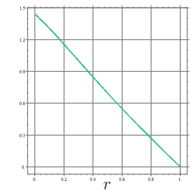
(b) $p=6$

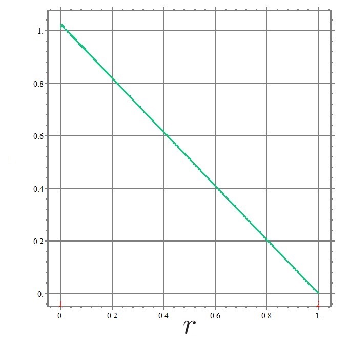
(c) $p=400$

Figure 2. Radial parts of eigenfunctions corresponding to the principal eigenvalue $\lambda(p)$ of $p$-Laplacian in the unit disc for ${p=1.3,6,400}$.

In the third case, we consider $p$ not equal to $q$. The performance of Algorithm 1 applied to system (5.1) with the initial guess $u_{0}=v_{0}=w_{1}$ is shown in Table 3 for various values of $p$, $q$, $\alpha$, and $\beta$. As an example, the pair of computed eigenfunction $(u,v)$ corresponding to $\lambda(30,2)$ is presented in Figure 3.

Table 3. The principal eigenvalue $\lambda(p,q)$ of system (1.1) in the unit circle computed by Algorithm 1 applied to system (5.1).

$p$	$q$	$\alpha$	$\beta$	$\lambda(p,q)$
30	1.5	1	1.4500	7.4486
30	2	1	1.9333	9.5034
30	5	1	4.8333	25.656
30	7	1	6.7666	40.194
30	10	1	9.6666	67.562
30	13	1	12.566	101.51
30	15	1	14.500	127.77
30	17	1	16.433	156.92
30	20	1	19.333	206.01
30	25	1	24.166	302.09

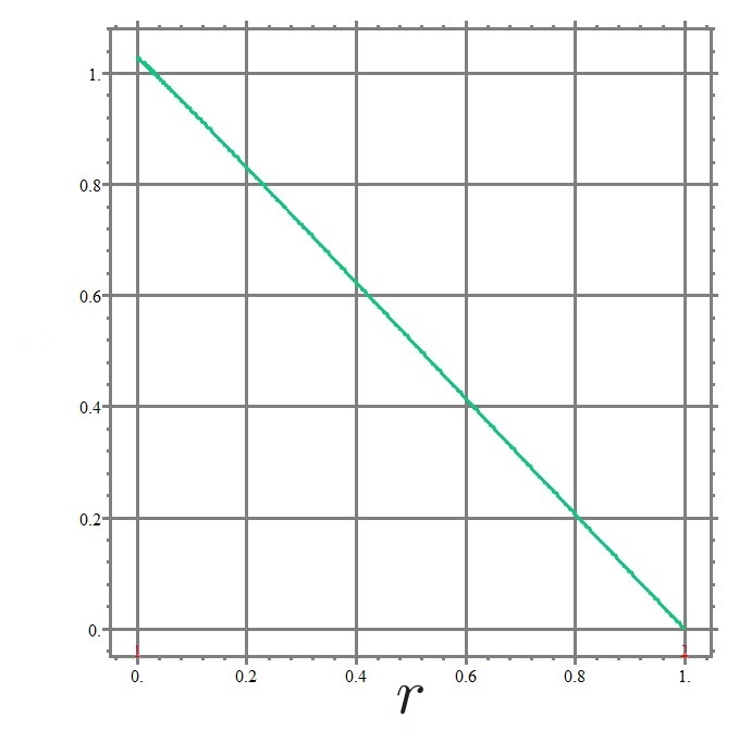
(a)

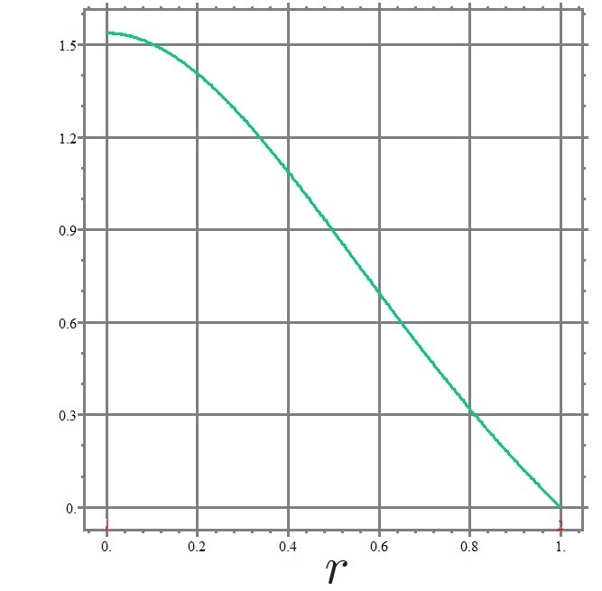
(b)

Figure 3. Radial parts of eigenfunctions $u$ (left) and $v$ (right) corresponding to $\lambda(30,2)$ with $\alpha=1$ and $\beta=1.9333$ for the unit disc.

Example 5.2.

In this example, we consider the square domain $\Omega=\{(x_{1},x_{2})\in\mathbb{R}^{2}:\>0<x_{1}<2,\>0<x_{2}<2\}$. The principal eigenvalue of system (1.1) corresponds to its main frequency and we apply Algorithm 1 to determine it for different values of $p$ and $q$. Table 4 lists the resulting principal eigenvalues for a mesh with 2390 elements, 4904 nodes, and mesh size $h=1/16=0.0625$.

Table 4. Principal eigenvalues of (1.1) in the square.

$p$	$q$	$\alpha$	$\beta$	$\lambda(p,q)$
10	1.5	1	1.35	6.0294
10	2	1	1.80	7.3695
10	3	1	2.70	10.173
10	4	1	3.60	13.183
10	5	1	4.50	16.391
10	6	1	5.60	19.788
10	7	1	6.30	23.356
10	8	1	7.20	27.076
10	9	1	8.10	30.957
10	10	1	9.00	34.999

A typical pair of eigenfunctions $(u,v)$ computed by Algorithm 1 is illustrated in Figure 4 for $p=10$, $q=2$, $\alpha=1$, and $\beta=1.8$.

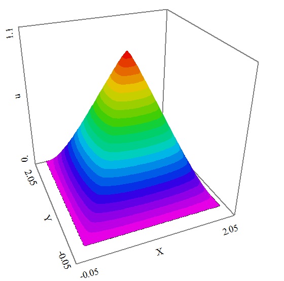
(a) $u$

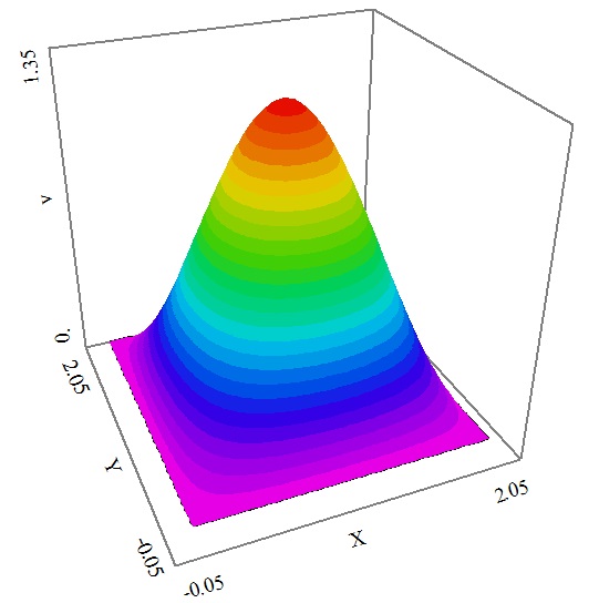
(b) $v$

Figure 4. Eigenpair $(u,v)$ corresponding to $\lambda(10,2)$ with ${\alpha=1,\>\beta=1.8}$.

Further, to demonstrate the accuracy of computed approximations we test the order of convergence of the used finite element method. We solve the problem on a sequence of successively refined meshes and we compute the experimental order of convergence $EOC$ using the ratio of successive differences of eigenvalues for different mesh sizes as

$$EOC=\log_{2}\left|\frac{\lambda_{h}-\lambda_{\frac{h}{2}}}{\lambda_{\frac{h}{2}}-\lambda_{\frac{h}{4}}}\right|.$$

We present it in Table 5 for $p=10$, $\alpha=1$, $q=1.5,5$, and $10$. The corresponding values of $\beta$ are given by (1.2) to be $1.35$, $4.50$, and $9$, respectively.

Table 5. Experimental orders of convergence $EOC$ for the square domain with $p=10$, $\alpha=1$, and $q=1.5,5$, and $10$.

$n$	$h=\frac{1}{2^{n}}$	$\lambda_{h}(10,1.5)$	$EOC$	$\lambda_{h}(10,5)$	$EOC$	$\lambda_{h}(10,10)$	$EOC$
$0$	1	6.48002	3.2308	20.9681	2.0802	69.4507	2.1857
$1$	$\frac{1}{2}$	6.08031	2.5340	17.1136	2.1573	42.3979	2.3063
$2$	$\frac{1}{4}$	6.03774	2.9234	16.5020	3.7281	36.4513	2.2662
$3$	$\frac{1}{8}$	6.03039		16.4064	3.0514	35.2491	2.7465
$4$	$\frac{1}{16}$	6.02942		16.3910		34.9992
$5$	$\frac{1}{32}$			16.3891		34.9619

The expected order of convergence is two. The higher experimental orders of convergence observed in Table 5 probably indicate the preasymptotic regime. On finer meshes the experimental order of convergence will probably decrease to values around two.

Example 5.3.

Here we test Algorithm 1 for three other domains, namely for an isosceles triangle, L-shaped domain, and a heart shaped domain. Note that L-shaped and heart shaped domains are non-convex and singularities of eigenfunctions are expected in re-entrant corners. To be more specific, the isosceles triangle has base 1 and altitude 1, the L-shaped domain is $(0,3)^{2}\setminus[1,3]^{2}$, and the heart shaped domain is $H=H_{1}\cup H_{2}\cup H_{3}$ where

$$H_{1} =\{(x,y)\in\mathbb{R}^{2}:\quad(x-1)^{2}+(y^{2}/4)<1,y\geq 0\},$$

$$H_{2} =\{(x,y)\in\mathbb{R}^{2}:\quad(x+1)^{2}+(y^{2}/4)<1,y\geq 0\},$$

$$H_{3} =\{(x,y)\in\mathbb{R}^{2}:\quad({x^{2}}/{4})+({y^{2}}/{16})<1,y\leq 0\}.$$

Table 6 lists the principal eigenvalues computed by Algorithm 1 for these three domains and different values of $p$ and $q$. The mesh size in all three cases was $h=1/16=0.0625$. For illustration we also present eigenfunctions $(u,v)$ corresponding to the principal eigenvalue $\lambda(3,10)$ and $\alpha=1$ and $\beta=6.6666$ in Figures 5–7 for the isosceles triangle, L-shaped domain, and the heart shaped domain, respectively.

Table 6. The principal eigenvalue for the isosceles triangle, L-shaped domain and heart shaped domain.

				$\lambda(p,q)$
$p$	$q$	$\alpha$	$\beta$	triangle	L-shape	heart
3	2	1	1.3333	$7.9822\times 10^{1}$	12.914	1.3330
3	3	1	2.0000	$2.2725\times 10^{2}$	23.632	1.1917
3	4	1	2.3333	$6.1966\times 10^{2}$	41.713	1.0268
3	5	1	3.3333	$1.6384\times 10^{3}$	71.810	0.8607
3	6	1	4.0000	$4.2386\times 10^{3}$	121.29	0.7061
3	7	1	4.6666	$1.0778\times 10^{4}$	201.73	0.5692
3	8	1	5.3333	$2.7038\times 10^{4}$	331.44	0.4523
3	9	1	6.0000	$6.7066\times 10^{4}$	539.05	0.3557
3	10	1	6.6666	$1.6479\times 10^{5}$	862.16	0.2766

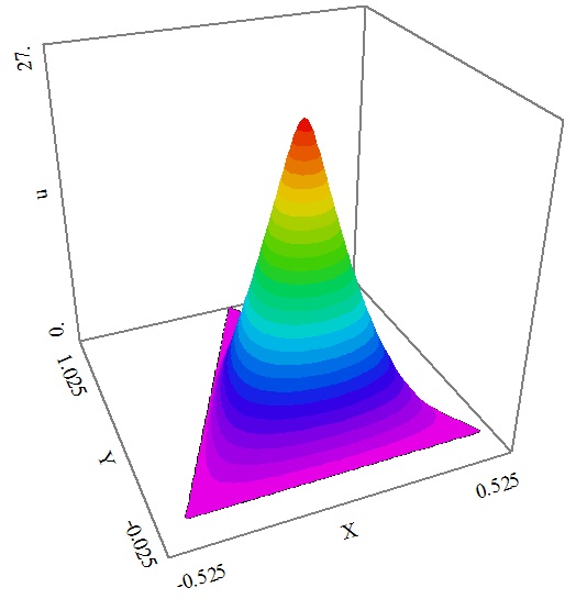
(a) $u$

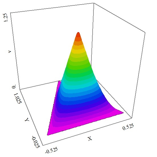
(b) $v$

Figure 5. Eigenfunctions $u$ (left) and $v$ (right) corresponding to $\lambda(3,10)$ with ${\alpha=1}$ and $\beta=6.6666$ for the isosceles triangle.

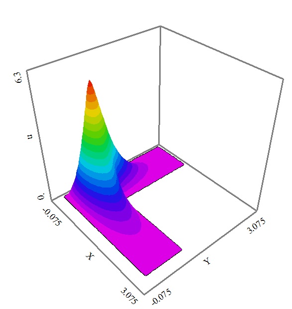
(a) $u$

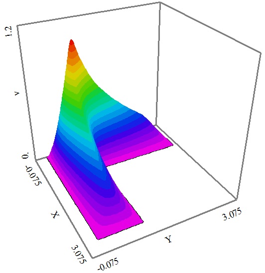
(b) $v$

Figure 6. Eigenfunctions $u$ (left) and $v$ (right) corresponding to $\lambda(3,10)$ with ${\alpha=1}$ and $\beta=6.6666$ for the L-shaped domain.

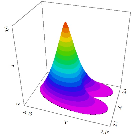
(a) $u$

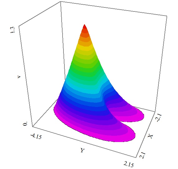
(b) $v$

Figure 7. Eigenfunctions $u$ (left) and $v$ (right) corresponding to $\lambda(3,10)$ with ${\alpha=1}$ and $\beta=6.6666$ for the heart shaped domain.

Example 5.4.

In order to present the usage of Algorithm 1 for a more general quasilinear system as it was proposed at the end of Section 4, we consider in this example a resonant quasilinear system of the following form

$$\left\{\begin{array}[]{lrl}-\Delta_{p}u=\Lambda(p,q)r(x)\alpha|u|^{\alpha-2}u|v|^{\beta}&\text{in }\Omega,\\ -\Delta_{q}v=\Lambda(p,q)r(x)\beta|u|^{\alpha}|v|^{\beta-2}v&\text{in }\Omega,\\ u=v=0&\text{on }\partial\Omega,\end{array}\right.$$ (5.2)

where $r\in L^{\infty}(\Omega)$ is a strictly positive function, $r(x)\geq m>0$. This system has been studied intensively by several authors, see e.g. [4, 5, 10, 25] to list just a few references.

The resonant quasilinear system (5.2) differs from (1.1) and has certain specific properties. For instance, in contrast to (1.1), the solution of system (5.2) does not satisfy $u=v$ for $p=q$. However, Algorithm 1 with above mentioned generalizations can be successfully used to compute its principal eigenvalues and eigenfunctions.

For illustration we consider the square ${\Omega=\{(x_{1},x_{2})\in\mathbb{R}^{2}:\>0<x_{1}<2,\>0<x_{2}<2\}}$ and function

$$r(x_{1},x_{2})=\left\{\begin{array}[]{lrl}1&\text{for }0<x_{1}\leq 1,\\ 2&\text{for }1<x_{1}<2.\\ \end{array}\right.$$

Principal eigenvalues $\Lambda(p,q)$ (corresponding to main frequencies) of system (5.2) computed by the generalized Algorithm 1 for different values of $p,q,\alpha$ and $\beta$ are listed in Table 7. The used mesh is the same as in Example 5.2.

Table 7. The principal eigenvalue of the resonant quasilinear system (5.2) on a square.

$p$	$q$	$\alpha$	$\beta$	$\Lambda(p,q)$	Upper bound (5.3)
10	2	1	1.80	4.6239	24.1474
10	3	1	2.70	4.3660	31.2932
10	4	1	3.60	4.3459	32.9794
10	5	1	4.50	4.4108	29.1125
10	6	1	5.40	4.5119	22.1799
10	7	1	6.30	4.6327	15.0333
10	8	1	7.20	4.7612	9.4046
10	9	1	8.10	4.8968	5.7214
10	10	1	9.00	5.0362	—

We note that in [4, 25], the following upper bound on the first eigenvalue of system (5.2) with $p>q$ has been found:

$$\Lambda(p,q)\leq\frac{\Lambda(p)}{p}+\frac{m^{-1+q/p}}{q}\left(\frac{p}{q}\right)^{q}(\Lambda(p))^{q/p},$$ (5.3)

where $\Lambda(p)$ is the first eigenvalue of the Dirichlet weighted $p$-Laplace eigenvalue problem

$$-\Delta_{p}u=\Lambda(p)r(x)|u|^{p-2}u\quad\text{in }\Omega.$$ (5.4)

Numerical results presented in the last column of Table 7 show that upper bound (5.3) may considerably overestimate the true eigenvalue for some values of parameters $p,q,\alpha$ and $\beta$.

Numerical results presented in Table 7 also show that the lower bound derived in Theorem 3.3 for the first eigenvalue of (1.1) cannot be straightforwardly generalized to system (5.2). For example, the value $\Lambda(10,4)=4.3459$ from Table 7 is not above $\Lambda(4)=5.7534$ nor $\Lambda(10)=18.1873$.

6. Conclusions

In this paper, an elliptic eigenvalue system involving the $p$-Laplace operator has been considered. The principal eigenvalue and corresponding eigenfunctions of the system have been investigated both analytically and numerically. We have provided an alternative proof for the simplicity of the principal eigenvalue and we have shown that this system reduces to the $p$-Laplace eigenvalue problem for a special choice of parameters. Further, we developed a numerical algorithm in order to compute approximate principal eigenvalues and corresponding eigenfunctions. We showed how to generalize this algorithm for gradient type systems. The convergence of this algorithm was verified numerically for various examples, but an analytical proof of convergence seems to be an interesting and difficult mathematical problem.

References

- [1] A. Anane, Simplicité et isolation de la première valeur propre du -Laplacien avec poids. C.R. Acad. Sci. Paris Stér. I Math. 305 (1987) 725–728.
- [2] K.L. Arruda, F.O. De Paiva, I. Marques, A remark on multiplicity of positive solutions for a class of quasilinear elliptic systems. In: Wei Feng, Zhaosheng Feng, Maurizio Grasselli, Akif Ibragimov, Xin Lu, Stefan Siegmund and Jürgen Voigt (eds), Dynamical Systems and Differential Equations, AIMS Proceedings 2011, pp. 112–116.
- [3] M. Belloni, B. Kawohl, A direct uniqueness proof for equations involving the -Laplace operator. Manuscripta Math. 109 (2002) 229–231.
- [4] L. Boccardo, D.G. de Figueiredo, Some remarks on a system of quasilinear elliptic equations. NoDEA Nonlinear Differential Equations Appl. 9 (2002) 309–323.
- [5] J. F. Bonder, J. P. Pinasco, Estimates for eigenvalues of quasilinear elliptic systems. Part II, J. Differential Equations 245 (2008) 875–891.
- [6] J. F. Bonder, J. P. Pinasco, Precise asymptotic of eigenvalues of resonant quasilinear systems. J. Differential Equations 249 (2010) 136–150.
- [7] C. Borell, Inverse Hölder inequalities in one and several dimensions, J. Math. Anal. Appl. 41 (1973) 300–312.
- [8] V. Bobkov, Y. Il’Yasov, Asymptotic behaviour of branches for ground states of elliptic systems. Electron. J. Differential Equations, no. 212, (2013) 1–21.
- [9] V. Bobkov, V., Y. Il’Yasov, Maximal existence domains of positive solutions for two-parametric systems of elliptic equations. Complex Var. Elliptic Equ. 61(5) (2016) 587–607.
- [10] L. M. Del Pezzo, J. D. Rossi, The first nontrivial eigenvalue for a system of -Laplacians with Neumann and Dirichlet boundary conditions. Nonlinear Anal. 137 (2016) 381–401.
- [11] F. Bozorgnia, Convergence of inverse power method for first eigenvalue of -Laplace Operator, Numer. Func. Anal. Opt. 37 (2016) 1378–1384.
- [12] J. Horak, Numerical investigation of the smallest eigenvalues of the -Laplace operator on planar domains, Electron. J. Differential Equations, no. 132, (2011) 1–30.
- [13] R. Hynd, E. Lindgren, Inverse iteration for p-ground states, Proc. Amer. Math. Soc. 144 (2016) 2121–2131.
- [14] R. Hynd, E. Lindgren, Approximation of the least Rayleigh quotient for degree p homogeneous functionals. J. Funct. Anal. 272 (2017) 4873–4918.
- [15] B. Kawohl, V. Fridman, Isoperimetric estimates for the first eigenvalue of the -Laplace operator and the Cheeger constant. Comment. Math. Univ. Carolin. 44 (2003) 659–667.
- [16] B. Kawohl, T. Lachand-Robert, Characterization of Cheeger sets for convex subsets of the plane. Pacific J. Math. 225 (2006) 103–118.
- [17] A. El. Khalil, S. El. Manouni, M. Ouanan, Simplicity and stability of the first eigenvalue of a nonlinear elliptic system. Int. J. Math. Math. Sci. 10 (2005) 1555–1563.
- [18] A. Lê, Eigenvalue problems for the -Laplacian, Nonlinear Anal. 64 (2006) 1057–1099.
- [19] P. Lindqvist, A nonlinear eigenvalue problem. In: Paolo Ciatti, Eduardo Gonzalez, Massimo Lanza de Cristoforis, Gian Paolo Leonardi (eds.), Topics in mathematical analysis, World Sci. Publ., Hackensack, NJ, 2008, pp. 175–203.
- [20] P. Lindqvist, On the equation . Proc. Amer. Math. Soc. 109 (1990) 157–164.
- [21] P. Lindqvist, Notes on -Laplace equation. University of Jyväskylä-Lectures notes, 2006.
- [22] P. Lindqvist, On non-linear Rayleigh quotients. Potential Anal. 2 (1993) 199–218.
- [23] A. Mohammadi, F. Bahrami, A nonlinear eigenvalue problem arising in a nanostructured quantum dot. Commun. Nonlinear Sci. Numer. Simul. 19 (2014) 3053–3062.
- [24] S. A. Mohammadi, H. Voss, A minimization problem for an elliptic eigenvalue problem with nonlinear dependence on the eigenparameter. Nonlinear Anal. Real World Appl. 31 (2016) 119–131.
- [25] P. L. De Nápoli, J. P. Pinasco, Estimates for eigenvalues of quasilinear elliptic systems. J. Differential Equations 227 (2006) 102–115.
- [26] J. L. Vàzquez, A strong maximum principle for some quasilinear elliptic equations. Appl. Math. Optim. 12 (1984) 191–202.
- [27] N. B. Zographopoulos, On the principal eigenvalue of degenerate quasilinear elliptic systems. Math. Nachr. 281 (2008) 1351–1365.