Explorative gradient method for active drag reduction of the fluidic pinball and slanted Ahmed body

Abstract

We address a challenge of active flow control: the optimization of many actuation parameters guaranteeing fast convergence and avoiding suboptimal local minima. This challenge is addressed by a new optimizer, called explorative gradient method (EGM). EGM alternatively performs one exploitive downhill simplex step and an explorative Latin hypercube sampling iteration. Thus, the convergence rate of a gradient based method is guaranteed while, at the same time, better minima are explored. For an analytical multi-modal test function, EGM is shown to significantly outperform the downhill simplex method, the random restart variant, Latin hypercube sampling, Monte Carlo iterations and the genetic algorithm.

EGM is applied to minimize the net drag power of the two-dimensional fluidic pinball benchmark with three cylinder rotations as actuation parameters. The net drag power is reduced by 40 % employing direct numerical simulations at a Reynolds number of $100$ based on the cylinder diameter. This optimal actuation leads to 98 % drag reduction employing Coanda forcing for boat tailing and partial stabilization of vortex shedding. The price is an actuation energy corresponding to 58% of the unforced parasitic drag power.

EGM is also used to minimize drag of the $35^{\circ}$ slanted Ahmed body employing distributed steady blowing with 10 inputs. 17% drag reduction are achieved using Reynolds-Averaged Navier-Stokes simulations (RANS) at the Reynolds number $Re_{H}=1.9\times 10^{5}$ based on the height of the Ahmed body. The wake is controlled with seven local jet slot actuators at all trailing edges. Symmetric operation corresponds to five independent actuator groups at top, midle, bottom, top sides and bottom sides. Each slot actuator produces a uniform jet with the velocity and angle as free parameters, yielding 10 actuation parameters as free inputs. The optimal actuation emulates boat tailing by inward-directed blowing with velocities which are comparable to the oncoming velocity. We expect that EGM will be employed as efficient optimizer in many future active flow control plants.

1 Introduction

In this study, we propose an optimizer for active flow control focusing on multi-actuator bluff-body drag reduction. This optimizer combines the convergence rate of a gradient-based method with an explorative method for identifying the global minimum. Actuators and sensors become increasingly cheaper, powerful and reliable. This trend makes active flow control of increasing interest to industry. In addition, distributed actuation can give rise performance benefits over single actuator solutions. Here, we focus on the simple case of open-loop control with steady or periodic operation of multiple actuators.

Even for this simple case, the optimization of actuation constitutes an algorithmic challenge. Often the budget for optimization is limited to $O(100)$ high fidelity simulations, like direct numerical simulations (DNS) or large-eddy simulations (LES) or $O(100)$ water tunnel experiments, or $O(1000)$ Reynolds Averaged Navier-Stokes (RANS) simulations, or a similar amount of wind-tunnel experiments. Moreover, the optimization may need to be performed for multiple operating conditions.

Evidently, efficient optimizers are of large practical importance. Gradient-based optimizers, like the downhill simplex method have the advantage of rapid convergence against a cost minimum, but this minimum may easily be a suboptimal local one, particularly for high-dimensional search spaces. Random restart variants have a larger probability of finding the global minimum but come with a dramatic increase of testing. In contrast to gradient-based approaches, Latin hypercube sampling performs an ideal exploration by guaranteeing a close geometric coverage of the search space—obviously with a poor associated convergence rate and the price of extensive evaluations of unpromising territories. Monte Carlo sampling has similar advantages and disadvantages. Genetic algorithms elegantly combine exploration with mutation and exploitation with crossover operations. These are routinely used optimizers and the focus of our study.

Myriad of other optimizers have been invented for different niche applications. Deterministic gradient-based optimizers may be augmented by estimators for the gradient. These estimators become particularly challenging for sparse data. This challenge is addressed by stochastic gradient methods which aim at navigating through a high-dimensional search space with insufficient derivative information. Many biologically inspired optimization methods, like ant colony and participle swarm optimization also aim at balancing exploitation and exploration, like the genetic algorithm. A new avenue is opened by including the learning of the response model from actuation to cost function during the optimization process and using this model for identifying promising actuation parameters. Another new path is ridgeline inter- or extrapolation (Fernex et al., 2020), exploiting the topology of the control landscape. In this study, these extensions are not included in the comparative analysis, as the additional complexity of these methods with many additional tuning parameters can hardly be objectively performed.

Our first flow control benchmark is the fluidic pinball (Ishar et al., 2019; Deng et al., 2020). This two-dimensional flow around three equal, parallel, equidistantly placed cylinders can be changed by the three rotation velocities of the cylinders. The dynamics is rich in nonlinear behaviour, yet geometrically simple and physically interpretable. With suitable rotation of the cylinders many literature-known wake stabilizing and drag-reducing mechanisms can be realized: (1) Coanda actuation (Geropp, 1995; Geropp & Odenthal, 2000), (2) circulation control (Magnus effect), (3) base bleed (Wood, 1964), (4) high-frequency forcing (Thiria et al., 2006), (5) low-frequency forcing (Glezer et al., 2005) and (6) phasor control (Protas, 2004). In this study, constant rotations are optimized for net drag power reduction accounting for the actuation energy. This search space implies the first three mechanisms. The fluidic pinball study will foreshadow key results of the Ahmed body. This includes the drag reducing actuation mechanism and the visualization tools for high-dimensional search spaces.

The main application focus of this study is on active drag reduction behind a generic car model using Reynolds-averaged Navier-Stokes (RANS) simulations. Aerodynamic drag is a major contribution of traffic-related costs, from airborne to ground and marine traffic. A small drag reduction would have a dramatic economic effect considering that transportation accounts for approximately $20\%$ of global energy consumption (Gad-el Hak, 2006; Kim, 2011). While the drag of airplanes and ships is largely caused by skin-friction, the resistance of cars and trucks is mainly caused by pressure or bluff-body drag. Hucho (2002) defines bodies with a pressure drag exceeding the skin-friction contribution as bluff and as streamlined otherwise.

The pressure drag of cars and trucks originates from the excess pressure at the front scaling with the dynamic pressure and a low-pressure region at the rear side of lower but negative magnitude. The reduction of the pressure contribution from the front side often requires significant changes of the aerodynamic design. Few active control solutions for the front drag reduction have been suggested (Minelli et al., 2020). In contrast, the contribution at the rearward side can significantly be changed with passive or active means. Drag reductions of 10% to 20% are common, (Pfeiffer & King, 2014) have even achieved 25% drag reduction with active blowing. For a car at a speed of 120 km/h, this would reduce consumption by about 1.8 liter per 100 km. The economic impact of drag reduction is significant for trucking fleets with a profit margin of only 2-3%. Two thirds of the operating costs are from fuel consumption. Hence, a 5% reduction of fuel costs from aerodynamic drag corresponds to over 100% increase of the profit margin.

The car and truck design is largely determined by practical and aesthetic considerations. In this study, we focus on drag reduction by active means at the rearward side. Intriguingly most drag reductions of bluff body fall in the categories of Kirchhoff solution and aerodynamic boat tailing. The first strategy may be idealized by the Kirchhoff solution, i.e. potential flow around the car with infinitely thin shear-layers from the rearward separation lines, separating the oncoming flow and a dead-water region. The low-pressure region due to curved shear-layers is replaced by an elongated, ideally infinitely long wake with small, ideally vanishing curvature of the shear-layer. Thus, the pressure of the dead water region is elevated to the outer pressure, i.e., the wake does not contribute to the drag. This wake elongation is achieved by reducing entrainment through the shear-layer, e.g. by phasor-control control mitigating vortex shedding (Pastoor et al., 2008) or by energetization of the shear-layer with high-frequency actuation (Barros et al., 2016). Wake disrupters also decrease drag, yet by energetizing the shear layer (Park et al., 2006) or delaying separation (Aider et al., 2010). Arguably, the drag of the Kirchhoff solution can be considered as achievable limit with small actuation energy.

The second strategy targets drag reduction by aerodynamic boat tailing. Geropp (1995); Geropp & Odenthal (2000) have pioneered this approach by Coanda blowing. Here, the shear-layer originating at the bluff body is vectored inward and gives thus rise to a more streamlined wake shape. Barros et al. (2016) has achieved 20% drag reduction of a square-back Ahmed body with high-frequency Coanda blowing in a high-Reynolds-number experiment. A similar drag reduction was achieved with steady blowing but at higher $C_{\mu}$ values.

This study focuses on drag reduction of the low-drag Ahmed body with rear slant angle of 35 degrees. This Ahmed body idealizes the shape of many cars. Bideaux et al. (2011); Gilliéron & Kourta (2013) have achieved 20% drag reduction for this configuration in an experiment. High-frequency blowing was applied orthogonal to the upper corner of the slanted rear surface. Intriguingly, the maximum drag reduction was achieved in a narrow range of frequencies and actuation velocities and its effect rapidly deteriorated for slightly changed parameters. In addition, the actuation is neither Coanda blowing nor an ideal candidate for shear-layer energization.

The literature on active drag reduction of the Ahmed body indicates that small changes of actuation can significantly change its effectiveness. Actuators have been applied with beneficial effects at all rearward edges (Barros et al., 2016), thus further complicating the optimization task. A systematic optimization of the actuation at all edges, including amplitudes and angles of blowing, is beyond reach of current experiments. In this study, a systematic RANS optimization is performed in a rich parametric space comprising the angles and amplitudes of steady blowing of five actuator groups: one on the top, middle and bottom edge and two symmetric actuators at the corners of the slanted and vertical surface. High-frequency forcing is not considered, as the RANS tends to be overly dissipative to the actuation response.

The manuscript is organized as follows. The employed optimization algorithms are introduced in § 2 and compared in § 3. § 4 optimizes the net drag power for the fluidic pinball, which features 2-dimensional flow controlled in a three-dimensional actuation space based on DNS. A simulation-based optimization of actuation for the three-dimensional low-drag Ahmed body is given in § 5. Here, up to 10 actuation commands controlling the velocity and direction of five rearward slot actuator groups are optimized. Our results are summarized in § 6.

2 Optimization algorithms

In this section, the employed optimization algorithms for the actuation parameters are described. Let $J(\bm{b})$ be the cost function—here the drag coefficient—depending on $N$ actuation parameters $\bm{b}=(b_{1},\ldots,b_{N})$ in the domain $\Omega$,

$$\bm{b}=[b_{1},\ldots,b_{N}]^{\rm T}\in\Omega\subset{\cal R}^{N},$$ (1)

there the superscript ‘$\rm T$’ denotes the transpose. Permissible values of each parameter define an interval, $b_{i}\in\left[b_{i,\rm min},b_{i,\rm max}\right]$, $i=1,\ldots,N$. In other words, optimization is performed in rectangular search space,

$$\Omega=\left[b_{1,\rm min},b_{1,\rm max}\right]\times\ldots\times\left[b_{N,\rm min},b_{N,\rm max}\right].$$ (2)

The optimization goal is to find the global minimum of $J$ in $\Omega$,

$$\bm{b}^{\star}=\arg\min\limits_{b\in\Omega}J(\bm{b}).$$ (3)

Several common optimization methods are investigated. Benchmark is the Downhill Simplex Method (DSM) (see, e.g., Press et al., 2007) as robust data-driven representative for gradient-based method (§ 2.4). This algorithm exploits gradient information from neighboring points to descent to a local minimum. Depending on the initial condition, this search may yield any local minimum. In the random restart simplex (RRS) method, the chance for finding a global minimum is increased by multiple runs with random initial conditions. The geometric coverage of the search space is the focus of Latin Hypercube Sampling (LHS) (see, again, Press et al., 2007), which optimally explores the whole domain $\Omega$ independently of the cost values, i.e., ignores any gradient information. Evidently, LHS has the larger chance of getting close to the global minimum while the simplex algorithm is more efficient in descending to a minimum, potentially a suboptimal one. Monte Carlo Sampling (MCS) (see, again, Press et al., 2007), is a simpler and more common exploration strategy by taking random values for each argument, again, ignoring any cost value information. Genetic Algorithms (GA) start with an MCS in the first generation but then employ genetic operations to combine explorative and exploitive features in the following generations (see, e.g., Wahde, 2008).

Sections 2.1–2.3 outline the non-gradient based explorative methods from the most explorative Latin hypercube sampling, to Monte Carlo sampling and the partially exploitive genetic algorithm. Sections 2.4 & 2.5 recapitulate the downhill simplex method and its random restart variant. These are commonly used methods for data-driven optimization with unknown analytical cost function.

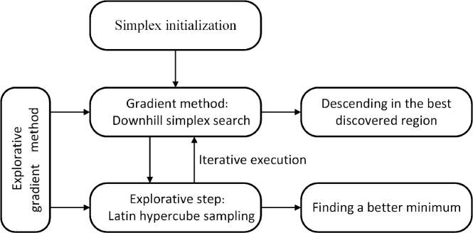
Figure 1: Sketch of the explorative gradient method. For details, see text.

In section 2.6, we combine the advantages of the simplex method in exploiting a local minimum and of the LHS in exploring the global one in a new explorative gradient method by an alternative execution (see figure 1). § 2.7 discusses auxiliary accelerators which are specific to the performed computational fluid dynamics optimization.

2.1 Latin hypercube sampling—Deterministic exploration

While our DSM benchmark exploits neighborhood information to slide down to a local minimum, Latin Hypercube Sampling (LHS) (McKay et al., 1979) aims to explore the parameter space irrespective of the cost values. We employ a space-filling variant which effectively covers the whole permissible domain of parameters. This explorative strategy (‘maximin’ criterion in Mathematica) minimizes the maximum minimal distance between the points:

$$\left\{\bm{b}_{m}\right\}_{m=1}^{M}=\arg\max\limits_{\bm{b}_{m}\in\Omega}\min\limits_{i=1,\ldots,M-1,\atop j=i+1,\ldots,M}\left\|\bm{b}_{i}-\bm{b}_{j}\right\|.$$

In other words, there is no other sampling of $M$ parameters with a larger minimum distance. $M$ can be any positive integral number.

For better comparison with the simplex algorithm, we employ an iterative variant. Note that once $M$ sample points are created they cannot be augmented anymore, for instance when learning by LHS was not satisfactory. We create a large number of LHS candidates $\bm{b}^{\star}_{j}$, $j=1,\ldots,M^{\star}$ for a dense coverage of the parameter space $\Omega$ at the beginning, typically $M^{\star}=10^{6}$. As first sample $\bm{b}_{1}$, the center of the initial simplex is taken. The second parameter is taken from $\bm{b}^{\star}_{j}$, $j=1,\ldots,M^{\star}$ maximizing the distance to $\bm{b}_{1}$,

$$\bm{b}_{2}=\hbox{argmax}_{j=1,\ldots,M^{\star}}\|\bm{b}^{\star}_{j}-\bm{b}_{1}\|.$$

The third parameter $\bm{b}_{3}$ is taken from the same set so that the minimal distance to $\bm{b}_{1}$ and $\bm{b}_{2}$ is maximized and so on. This procedure allows to recursively refine sample points and to start with an initial set of parameters.

2.2 Monte Carlo Sampling—Stochastic exploration

The employed space-filling variant of LHS requires the solution of an optimization problem guaranteeing a uniform geometric coverage of the domain. In high-dimensional domains, this coverage many not be achievable. A much easier and far more commonly used exploration strategy is Monte Carlo Sampling (MCS). Here, the $m$th sample $\bm{b}_{m}=\left[b_{1,m},\ldots,b_{N,m}\right]^{\rm T}$ is given by

$$b_{i,m}=b_{i,\rm min}+\zeta_{i,m}\left(b_{i,\rm max}-b_{i,\rm min}\right),$$ (4)

$\zeta_{i,m}\in[0,1]$ are random numbers with uniform probability distribution in the unit domain. The relative performance between LHS and MCS is a debated topic. We will wait for the results for an analytical problem in section 3.

2.3 Genetic algorithm—Biologically inspired exploration and exploitation

The Genetic Algorithm (GA) mimics natural selection process. We refer to Wahde (2008) as excellent reference. In the following, the method is briefly outlined to highlight the specific version and the chosen parameters.

Any parameter vector $\bm{b}=[b_{1},b_{2},\ldots,b_{N}]^{\rm T}\in\Omega\subset{\cal R}^{N}$ comprises the real values $b_{i}$, also called alleles. This real value is encoded as a binary number and called gene. The chromosome comprises alle genes and represents the parameter vector (Wright, 1991).

The genetic algorithm evolves one generation of $I$ parameters, also called individuals, into a new generation with the same number of parameters using biological inspired genetic operations. The first generation is based on MCS, i.e., represents completely random genoms. The individuals $J_{i}^{1}$, $i=1,\ldots,I$ are evaluated and sorted by their costs

$$J_{1}^{1}\leq J_{2}^{1}\leq\ldots\leq J_{I}^{1}.$$

The next generation is computed with elitism and two genetic operations. Elitism copies the $N_{e}$ best performing individuals in the new generation. $P_{e}=N_{e}/I$ denotes the relative quota. The two genetic operations include mutation, which randomly changes parts of the genom, and crossover, which randomly exchanging parts of the genoms of two individuals. Mutation serves explorative purposes and crossover has the tendency to breed better individuals. In an outer loop, the genetic operations are randomly chosen with probabilities $P_{m}$ and $P_{c}$ for mutation and crossover, respectively. Note that $P_{e}+P_{m}+P_{c}=1$ by design.

In the inner loop, i.e., after the genetic operation is determined, individuals from the current generation are chosen. Higher performing individuals have higher probability to be chosen. Following the genetic algorithm matlab routine, this probability is proportional to the inverse square-root of its relative rank $p\propto 1/\sqrt{i}$.

The genetic algorithm terminates according to a predetermined stop criterion, here a maximum number of generations $L$ or corresponding number of evaluations $M=IL$. For reasons of comparison, we renumber the individuals in the order of their evaluation, i.e., $m\in\{1,\ldots,I\}$ belongs to the first generation, $m\in\{I+1,\ldots,2I\}$ to the second generation, etc.

The chosen parameters are the default values of matlab, e.g. $P_{r}=0.05$ $P_{c}=0.8$, $P_{m}=0.15$, $N_{e}=3$. Further details are provided in the appendix A.

2.4 Downhill simplex search—A robust gradient method

The Downhill Simplex Method (DSM) by Nelder & Mead (1965) is a very simple, robust and widely used gradient method. This method does not require any gradient information and is well suited for expensive function evaluations, like the considered RANS simulation for the drag coefficients, and for experimental optimizations with inevitable noise. A price is a slow convergence for the minimization of smooth functions as compared to algorithms which can exploit gradient and curvature information.

We briefly outline the employed downhill simplex algorithm, as there are many variants. First, $N+1$ vertices $\bm{b}_{m}$, $m=1,\ldots,N+1$ in $\Omega$ are initialized as detailed in the respective sections. Commonly, $\bm{b}_{N+1}$ is placed somewhere in the middle of the domain and the other vertices explore steps in all directions, $\bm{b}_{m}=\bm{b}_{N+1}+h\>\bm{e}_{m}$, $m=1,\ldots,N$. Here, $\bm{e}_{i}=[\delta_{i1},\ldots,\delta_{iN}]^{\rm T}$ is a unit vector in $i$-th direction and $h$ is a step size which is small compared to the domain. Evidently, all vertices must remain in the domain $\bm{b}_{m}\in\Omega$.

The goal of the simplex transformation iteration is to replace the worst argument $\bm{b}_{h}$ of the considered simplex by a new better one $\bm{b}_{N+2}$. This is archived in following steps:

1) Ordering:

Without loss of generality, we assume that the vertices are sorted in terms of the cost values $J_{m}=J(\bm{b}_{m})$: $J_{1}\leq J_{2}\leq\ldots\leq J_{N+1}$.

2) Centroid:

In the second step, the centroid of the best side opposite to the worst vertex $\bm{b}_{N+1}$ is computed:

$$\bm{c}=\frac{1}{N}\sum\limits_{m=1}^{N}\bm{b}_{m}.$$

3) Reflection:

Reflect the worst simplex $\bm{b}_{N+1}$ at the best side,

$$\bm{b}_{r}=\bm{c}+\left(\bm{c}-\bm{b}_{N+1}\right)$$

and compute the new cost $J_{r}=J(\bm{b}_{r})$. Take $\bm{b}_{r}$ as new vertex, if $J_{1}\leq J_{r}\leq J_{N}$. $\bm{b}_{m}$, $m=1\ldots,N$ and $\bm{b}_{r}$ define the new simplex for the next iteration. Renumber the indices to the $1\ldots N+1$ range. Now, the cost is better than the second worst value $J_{N}$, but not as good as the best one $J_{1}$. Start a new iteration with step 1.

4) Expansion:

If $J_{r}<J_{1}$, expand in this direction further by a factor $2$,

$$\bm{b}_{e}=\bm{c}+2\left(\bm{b}_{N+1}-\bm{c}\right).$$

Take the best vertex of $\bm{b}_{r}$ and $\bm{b}_{e}$ as $\bm{b}_{N+1}$ replacement and start a new iteration.

5) Single contraction:

At this stage, $J_{r}\geq J_{N}$. Contract the worst vertex half-way towards centroid,

$$\bm{b}_{c}=\bm{c}+\frac{1}{2}\left(\bm{c}-\bm{b}_{N+1}\right).$$

Take $\bm{b}_{c}$ as new vertex ($\bm{b}_{N+1}$ replacement), if it is better than the worst one, i.e., $J_{c}\leq J_{N+1}$. In this case, start the next iteration.

6) Shrink / multiple contraction:

At this stage, none of the above operations was successful. Shrink the whole simplex by a factor $1/2$ towards the best vertex, i.e., replace all vertices by

$$\bm{b_{m}}\mapsto\bm{b}_{1}+\frac{1}{2}\>\left(\bm{b}_{m}-\bm{b}_{1}\right),m=2,\ldots,N+1.$$

This shrinked simplex represents the one for the next iteration. It should be noted that this shrinking operation is the last resort as it is very expensive with $N$ function evaluations. The rationale behind this shrinking is that a smaller simplex may better follow local gradients.

2.5 Random restart simplex method—Preparing for multiple minima

The downhill simplex method of the previous section may be equipped with a random restart initialization (Humphrey & Wilson, 2000). As random initial condition, we chose a Monte Carlo sample as main vertex of the simplex and explore all coordinate directions by a positive shift of 10% of the domain size. It is secured that all vertices are inside the domain $\Omega$. These initial simplexes attribute the same probability to the whole search space. The chosen small edge length makes a locally smooth behaviour probable—in absence of any other information. The downhill search is stopped after a fixed number of evaluations. We chose 50 evaluations as safe upper bound for convergence. It should be noted that the number of simplex iterations is noticeably smaller, as one iteration implies one to $N+2$ evaluations.

Evidently, the random restart algorithm may be improved by appreciating the many recommendations of literature, e.g., avoiding closeness to explored parameters. We trade these improvements in all optimization strategies for simplicity of the algorithms.

2.6 Explorative gradient method–Combining exploration and gradient method

In this section, we combine the advantages of the exploitive DSM and the explorative LHS in a single algorithm.

Step 0—Initialize.

First, $\bm{b}_{m}$, $m=1,\ldots,M+1$ are initialized for the DSM.

Step 1—Downhill simplex.

Perform one simplex iteration (§ 2.4) with the best $M+1$ parameters discovered so far.

Step 2—LHS.

Compute the cost $J$ of a new LHS parameter $\bm{b}$. As described above, we take a parameter from a precomputed list which is the furthest away from all hitherto employed parameters.

Step 3—Loop.

Continue with Step 1 until a convergence criterion is met.

Sometimes, the simplex may degenerate to one with small volume, for instance, when it crawls through a narrow valley. In this case, the vertices lie in a subspace and valuable gradient information is lost. This degeneration is diagnosed and cured after step 1 as follows. Let $\bm{b}_{c}$ be the geometric center of the simplex. Compute the distance $D$ between each vertex and their geometric center point. If the minimum ${D}_{\rm min}$ is smaller than half the maximum distance ${D}_{\rm max}/2$, the simplex is deemed degenerated. This degeneration is removed as follows. Draw a sphere with ${D}_{max}$ around the simplex center. This sphere contains all vertices by construction. Obtain $1000$ random points in this sphere. Replace the vertex with the highest cost $J_{max}$ with one of these point to create simplex with the largest volume. Of course, the cost of this changed point needs to be evaluated.

The algorithm is intuitively appealing. If the LHS discovers a parameter with a cost $J$ in the top $M+1$ values, this parameter is included in the new simplex and corresponding iteration may slide down in another better minimum. It should be noted that LHS exploration does not come with the toll of having to evaluate the cost at $N+1$ vertices and subsequent iterations. The downside of a single evaluation is that we miss potentially important gradient information pointing to an unexplored much better minimum. Relative to random-restart gradients searches requiring a many evaluations for a converging iteration, LHS exploration becomes increasingly better in rougher landscapes, i.e., more complex multi-modal behaviour.

2.7 Computational accelerators

The RANS based optimization may be accelerated by enablers which are specific to the chosen flow control problem. The computation time for each RANS simulation is based on the choice of the initial condition, as it affects the convergence time for the steady solution. The first simulation of an optimization starts with the unforced flow as initial condition. The next iterations exploit that the averaged velocity field $\overline{\bm{u}}(\bm{x})$ is a function of the actuation parameter $\bm{b}$. The initial condition of the $m$th simulation is obtained with the 1-nearest-neighbour approach: The velocity field associated with the closest hitherto computed actuation vector is taken as initial condition for the RANS simulation. This simple choice of initial condition saves about 60 % CPU time in reduced convergence time.

Another 30 % reduction of the CPU time is achieved by avoiding RANS computations with very similar actuations. This is achieved by a quantization of the $\bm{b}$ vector: The actuation velocities are quantized with respect to integral $\rm m/s$ values. This corresponds to increments of $U_{\infty}/30$ with $U_{\infty}=30\>\>\rm m/s$. All actuation vectors are rounded with respect to this quantization. If the optimization algorithm yields a rounded actuation vector which has already been investigated, the drag is taken from the corresponding simulation and no new RANS simulation is performed. Similarly, the angles are discretized into integral degrees.

3 Comparative optimization study

In this section, the six optimization methods of § 2 are compared for an analytical function with 4 local minima. § 3.1 describes this function. In § 3.2, the optimization methods with corresponding parameters are discussed. § 3.3 shows the tested individuals. The learning rates are detailed in § 3.4. Finally, the results are summarized (§ 3.5).

3.1 Analytical function

The considered analytical cost function

$$\begin{split}J(b_{1},b_{2})=1&\>\>-\>\>e^{-2(b_{1}-1)^{2}-2(b_{2}-1)^{2}}-\frac{1}{2}e^{-2(b_{1}+1)^{2}-2(b_{2}-1)^{2}}\\ &-\frac{1}{3}e^{-2(b_{1}-1)^{2}-2(b_{2}+1)^{2}}-\frac{1}{4}e^{-2(b_{1}+1)^{2}-2(b_{2}+1)^{2}}\end{split}$$ (5)

is characterized by a global minimum near $[1,1]^{\rm T}$ and three local minimum separately near $[1,-1]^{\rm T}$, $[-1,1]^{\rm T}$, and $[-1,-1]^{\rm T}$. The cost reaches a plateau $J=1$ far away from the origin. The investigated parameter domain is $\Omega=[-3,3]\times[-3,3]$.

3.2 Optimization methods and their parameters

Latin hypercube sampling (LHS) is performed as described in § 2.1. We take $M^{\star}=10^{3}$ random points for the optimization of the coverage. The Monte Carlo sampling (MCS) is uniformly distributed over the parameter domain $\Omega$.

The most important parameters of genetic algorithms (GA) are summarized from appendix A: The generation size is $I=50$ and the iterations are terminated with generation $L=20$. The crossover and mutation probabilities are $P_{c}=0.80$ and $P_{m}=0.15$, respectively. The number of elite individuals $N_{e}=3$ correspond to the probability complementary probability $P_{e}=5\>\%$.

The downhill simplex method follows exactly the description of § 2.4 with an expansion rate of $2$, single contraction rate of $1/2$ and a shrink rate of $1/2$. The random restart variant (RRS, § 2.5) has an evaluation limit of 50 for 20 random restarts. The step size for each initial simplex is $h=0.35$. The explorative gradient method (EGM) builds on the LHS and downhill simplex iterations discussed above.

3.3 Tested individuals in the parameter space

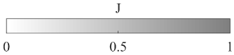
(a)

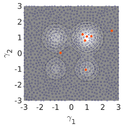
(a)

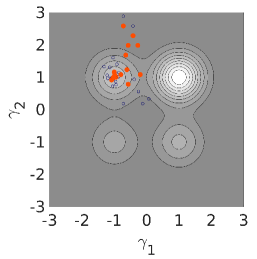
(b)

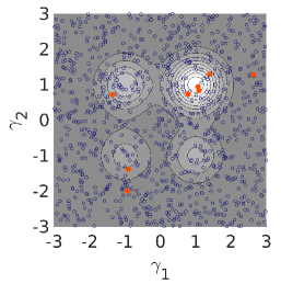
(c)

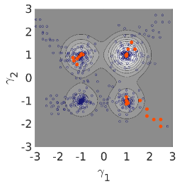
(d)

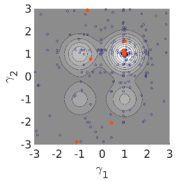
(e)

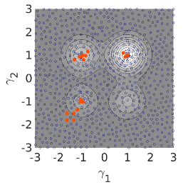
(f)

Figure 2: Comparison of all optimizers for the analytical function (5). Tested individuals of a) LHS, b) DSM, c) MCS, d) RRS, e) GA and f) EGM from a typical optimization with 1000 individuals. The red solid circles mark new local minima during the iteration while the blue open circles represent suboptimal tested parameters.

Figure 2 illustrates the iteration of all six algorithms in the parameter space. LHS shows a uniform coverage of the domain. In contrast, MCS leads to local ‘lumping’ of close individuals, i.e., indications of redundant testing, and local untested regions, both undesirable features. Thus, LHS is clearly seen to perform better than MCS. The genetic algorithm is seen to sparsely test the plateau while densely populating the best minima. This is clearly a desirable feature over LHS and MCS.

The standard downhill simplex method converges to a local minimum in this realization, while the random restart variant (RRS) finds all minima, including the global optimal one. Clearly, the random restart initialization is a security policy against sliding into a suboptimal minimum. The proposed new explorative gradient method (EGM) finds all four minima and converges against the global one. By construction, the exploration is less dense as LHS. The 1000 iterations comprise about 250 LHS steps and about 250 downhill simplex iterations with an average of 3 evaluations for each.

Arguably, the EGM is seen to be superior to all downhill simplex variant with more dense exploration and convergence to the global optimum. EGM also performs better than LHS, MCS, and genetic algorithm, as it invests in a more dense coverage of the parameter domain while about $75\>\%$ of the evaluations serve the convergence.

The conclusions are practically independent of the chosen realization of the optimization algorithm, except that the downhill simplex method slides into the global minimum in about $27\>\%$ of the cases.

We note that some of our conclusions are tied to the low dimension of the parameter space. In, cubical domain of 10 dimensions, the first $2^{10}=1024$ LHS individuals would populate the corners before the interior is explored. A geometric coverage of higher dimensions is incompatible with a budget of 1000 evaluations.

3.4 The learning curve

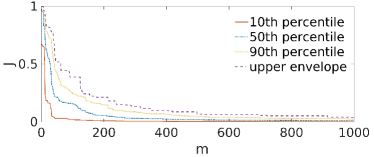
(a)

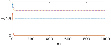
(b)

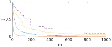
(c)

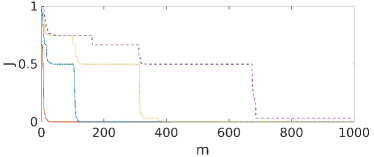
(d)

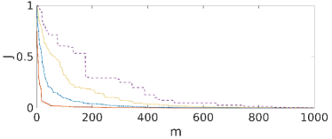
(e)

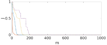
(f)

Figure 3: Comparison of all optimizers for the analytical function (5). Learning curve of (a) LHS, (b) Simplex, (c) Monte Carlo, (d) RRS, (e) GA and (f) EGM in 100 runs. $10th$, $50th$, and $90th$ percentile indicates the J value below which 10, 40 and 90 percentage of runs at current evaluation falls.

In figure 3, we investigate the learning curve of each algorithm for 100 realizations with randomly chosen initial conditions. The learning curve shows the best cost value found with $m$ evaluations. In this statistical analysis, the $10$, $50$ and $90\>\%$ percentiles of the learning curves are displayed. The $10\>\%$ percentile at $m$ evaluations implies that $10\>\%$ of the realizations yield better and $90\>\%$ yield worse cost values. The $50\>\%$ and $90\>\%$ percentiles are defined analogously.

The gradient-free algorithms (LHS, MC, GA) in the left column show smooth learning curves. All iterations eventually converge against the global optimum as seen from the upper envelope. The $10\>\%$ and $50\>\%$ percentile curves are comparable. Focusing on the bad case ($90\>\%$ percentile) and worst case performance (upper envelope), LHS is seen to beat both MCS and GA. MCS has the worst outliers, because it neither exploits the cost function, like the GA, nor comes with advantage of guaranteed good geometric coverage, like LHS.

The gradient-based algorithms reveal other features. The downhill simplex method can arrive at the global optimum much faster than any of the gradient-free algorithms. But is has also a $73\>\%$ probability terminating in one of the suboptimal local minima. The random restart version mitigates this risk to practically zero. In RRS, $50\>\%$ of the runs reach the minimum before 300 evaluations.

The learning curve of all gradient-based algorithms have jumps. Once the initial condition is in the attractive basin of one minimum, the convergence to that minimum is very fast, leading to a step decline of the learning curve. We notice that the worst case scenario does not exactly converge to zero. The reason is the degeneration of the simplex to points on a line which does not go through the global minimum. Only the EGM takes care of this degeneration with a geometric correction after step 1 as described in § 2.6. Expectedly, EGM also outperforms all other optimizers with respect to $50\>\%$ percentile, $90\>\%$ percentile and the worst case scenario. The global minimum is consistently found in less than 200 evaluations. It is much more efficient to invest 50 points in LHS exploration than to iterate into a suboptimal minimum. The price to be paid with EGM is that the best case performance is mitigated by gradient descent which is distracted by roughly $25\>\%$ LHS iterations as insurance policy.

3.5 Discussion

Method	Evaluation				Failure rate
	$20^{th}$	$100^{th}$	$500^{th}$	$1000^{th}$
LHS	0.5163	0.1456	0.0218	0.0129	0.55
MCS	0.4810	0.1863	0.0441	0.0221	0.61
GA	0.4269	0.1441	0.0065	0.0002	0
DSM	0.4893	0.4675	0.4673	0.4673	0.73
RRS	0.4893	0.3208	0.0211	0.0003	0.01
EGM	0.5121	0.0621	0.0000	0.0000	0

Table 1: Comparison of all optimizers for the analytical function (5). Average cost of different algorithms during $m=20$, $100$, $500$ and $1000$ evaluations in 100 runs.

The relative strengths and weaknesses of the different optimizers are summarized in table 1 for the average performance after $m=20$, $100$, $500$ and $1000$ evaluations. The averaging is performed over the costs of all 100 realizations after $m$ evaluations. The iteration is considered as failed if the value is $1\>\%$, i.e., $0.01$ above the global minimum.

First, we observe that the downhill simplex algorithm has the worst failure rate with $73\>\%$, followed by $61\>\%$ of MCS and $55\>\%$ of LHS. The failures of the simple simplex method are more severe as the converged parameters significantly depart from the global minimum in $73\>\%$ of the runs. In case of LHS and MCS, the failure is only the result of pure convergence against the right global minimum.

Second, after 20 evaluations, the average cost of all algorithms is close to $0.50$, i.e., very similar.

After 100 evaluations, algorithms with explorative steps, i.e., LHS, MCS, GA and EGM have a distinct advantage over the downhill simplex method and even over the random restart version. About 4 restarts are necessary to avoid the convergence to a suboptimal minimum in $99\>\%$ of the cases. EGM is already better than the other algorithms by a large factor.

After 500 evaluations, EGM corroborates its distinct superiority over the other algorithms, followed by the RRS and GA. Intriguingly, GA with its exploitive crossover operation performs better than all other optimizers after 500 evaluations, except for EGM. LHS and MCS keep a significant error, lacking gradient-based optimization.

Summarizing, algorithms combining exploration and exploitation, i.e., EGM, GA and RRS, perform better than purely explorative or purely exploitive algorithms (LHS, MCS and Simplex). For the ‘pure’ algorithms, LHS has the fastest decrease of cost function while simplex has the fastest convergence. EGM turns out to be the best combined algorithm by making a balance of exploration and exploit from LHS and simplex respectively. This superiority is already apparent after 100 evaluations.

We note that the conclusions have been drawn for a single analytical example for an optimization in a low-dimensional parameter space with few minima. From many randomly created analytical functions, we observe that EGM tends to outperform other optimizers in the case of few smooth minima and for low-dimensional search spaces. Yet, in higher-dimensional search spaces, LHS becomes increasingly inefficient and MCS may turn out to perform better. The number of minima also has an impact on the performance. For a single minimum with parabolic growth, the DSM can be expected to outperform the other algorithms. In case of many local shallow minima, the advantage of gradient-based approaches will become smaller and exploration will correspondingly increase in importance.

4 Drag optimization of fluidic pinball with three actuators

As first flow control example, the explorative gradient method is applied to the two-dimensional fluidic pinball (Deng et al., 2020; Cornejo Maceda et al., 2019), the wake behind a cluster of three rotating cylinders. In § 4.1, the benchmark problem is described: Minimize the net drag power with the cylinder rotations as input parameters. In § 4.2, the explorative gradient method yields a surprising non-symmetric result, consistent with other fluidic pinball simulations (Cornejo Maceda et al., 2019) and experiments (Raibaudo et al., 2019). The learning process of the Downhill Simplex Method (DSM) and Latin Hypercube Sampling (LHS) are investigated in § 4.3 and 4.4,

4.1 Configuration

The fluidic pinball is a benchmark configuration for wake control which is geometrically simple yet rich in nonlinear dynamics behaviours. This two-dimensional configuration consists of a cluster of three equal, parallel and equidistantly spaced cylinders pointing in opposite to uniform flow. The wake can be controlled by the cylinder rotation. The fluidic pinball comprises most known wake stabilization mechanisms, like phasor control, circulation control, Coanda forcing, base bleed as well as high and low-frequency forcing. In this study, we focus on steady open-loop forcing minimizing the drag power corrected by actuation energy.

The viscous incompressible two-dimensional flow has uniform oncoming flow with speed $U_{\infty}$ and a fluid with constant density $\rho$ and kinematic viscosity $\nu$. The three equal circular cylinders have radius $R$ and their centers form an equilateral triangle with sidelength $3R$ pointing upstream. Thus, the transverse dimension of the cluster reads $L=5R$.

In figure 4a, the flow is described in Cartesian coordinate system where the $x$-axis points in the direction of the flow, the $z$-axis is aligned with the cylinder axes and the $y$-axis is orthogonal to both. The origin $\bm{0}$ is placed in the center of the rightmost top and bottom cylinders. Thus, the centers of the cylinders are described by

$$\begin{array}[]{ll}x_{1}=x_{F}=-3\>R\>\cos 30^{\circ},&y_{1}=y_{F}=0,\\ x_{2}=x_{B}=0,&y_{2}=y_{B}=-3R/2,\\ x_{3}=x_{T}=0,&y_{3}=y_{T}=+3R/2.\end{array}$$ (6)

Here, the subscripts ‘F’, ‘B’ and ‘T’refer to the front, bottom and top cylinder. Alternatively, the subscripts ’1’, ’2’ and ’3’ are used for these cylinders starting with the front cylinder and continuing in mathematically positive orientation.

The location is denoted by $\bm{x}=(x,y)=x\>\bm{e}_{x}+y\>\bm{e}_{y}$, where $\bm{e}_{x}$ and $\bm{e}_{y}$ are the unit vectors in $x$- and $y$-direction. The flow velocity is represented by $\bm{u}=(u,v)=u\>\bm{e}_{x}+v\>\bm{e}_{y}$. The pressure and time symbols are $p$ and $t$, respectively. In the following, all quantities are non-dimensionalized with cylinder diameter $D=2R$, the velocity $U_{\infty}$ and the fluid density $\rho$.

The corresponding Reynolds number reads $Re_{D}=U_{\infty}D/\nu=100$. This Reynolds number corresponds to asymmetric periodic vortex shedding. Deng et al. (2020) have investigated the transition scenario for increasing Reynolds number. At $Re_{1}\approx 18$, the steady flow becomes unstable in a Hopf bifurcation leading to periodic vortex shedding. At $Re_{2}\approx 68$, both the steady Navier-Stokes solutions and the limit-cycles bifurcate into two mirror-symmetric states. Chen et al. (2020) performed a careful parametric analysis of the gap width between the cylinders and associated this behaviour with the ‘deflected regime’, where base bleed through the rightmost cylinder are deflected upward or downward. At $Re_{3}\approx 104$ another Hopf bifurcation leads to quasi-periodic flow. After $Re_{4}\approx 115$, a chaotic state emerges.

The flow properties can be changed by the rotation of cylinders. The corresponding actuation commands are denoted by

$$b_{1}=U_{F},\quad b_{2}=U_{B},\quad b_{3}=U_{T}.$$ (7)

Here, positive values denote the anti-clockwise direction.

Following Cornejo Maceda et al. (2019), we aim to minimize of the averaged parasitic drag power $\bar{J_{a}}$ penalizing the averaged actuation power $\bar{J_{b}}$. The resulting cost function reads

$$\bar{J}=\bar{J}_{a}+\bar{J}_{b}.$$ (8)

The first contribution $\bar{J}_{a}=c_{D}$ corresponds to drag coefficient

$$c_{D}=\frac{\bar{F}_{D}}{(1/2)\rho DU_{\infty}^{2}}$$ (9)

for the chosen non-dimensionalization. Here, $\bar{F}_{D}$ denotes total averaged drag force on all cylinders per unit spanwise length. The second contribution arises from the necessary actuation torque to overcome the skin-friction resistance.

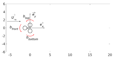
(a)

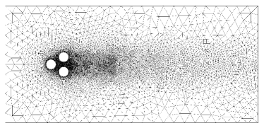
(b)

Figure 4: Fluidic pinball (a) configuration and (b) grid.

Following Deng et al. (2020), the flow is computed with direct numerical solution in the computational domain

$$\Omega=\{(x,y):-6\leq x\leq 20\wedge|y|\leq 6\wedge(x-x_{i})^{2}+(y-y_{i})^{2}\geq 1/4,i=1,2,3)\}.$$ (10)

We use an in-house implicit finite-element method solver ‘UNS3’ which is of third-order accuracy in space and time. The unstructured grid in figure 4b contains 4225 triangles and 8633 vertices. An earlier grid convergence study identified this resolution sufficient for up to 2 percent error in drag, lift and Strouhal number.

4.2 Optimized actuation

$m$	$b_{1}$	$b_{2}$	$b_{3}$	J
1	0	-3	3	4.9579
2	0.1	-3	3	4.9695
3	0	-2.9	3	4.8979
4	0	-3	3.1	5.0702

Table 2: Fluidic pinball: Initial simplex ($m=1,2,3,4$) for the three-dimensional downhill simplex optimization. $b_{i}$ denotes the circumferential velocity of cylinders and $J$ corresponds to the net drag power (8).

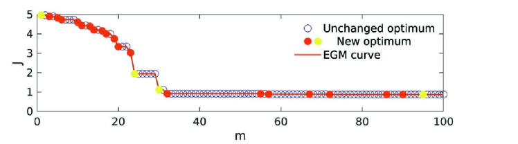
(a)

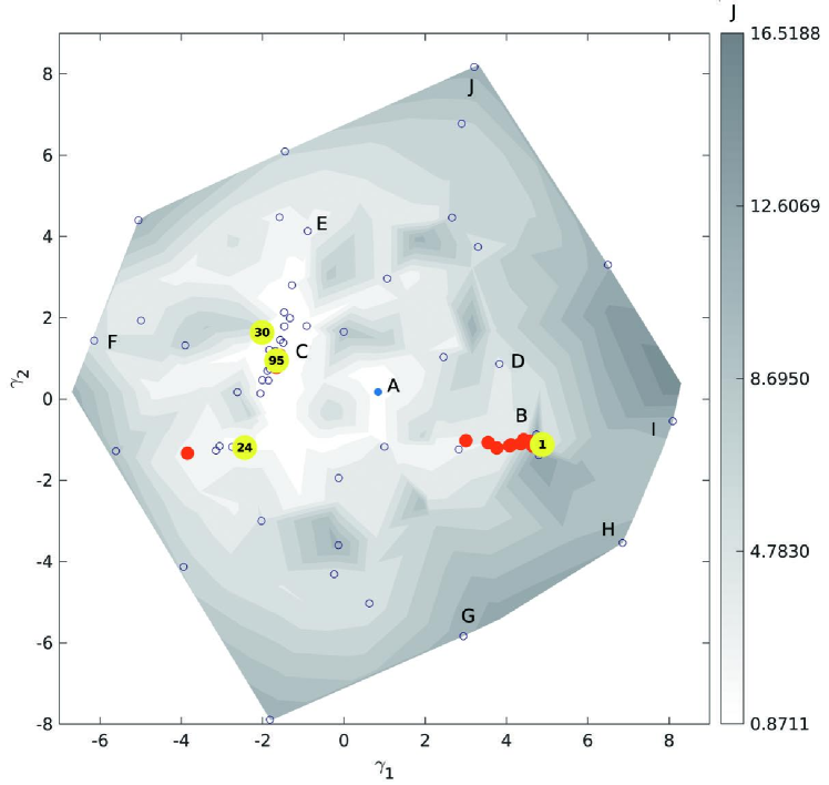
(b)

Figure 5: Optimization of the fluidic pinball actuation with EGM. The actuation parameters and costs are visualized like figure 2 and 3. For enhanced interpretability, selected new minima are displayed as solid yellow circles in the learning curve (a) and in the control landscape (b) corresponding to $m$. $m$ counts the direct numerical simulations for net drag power computation. The marked flows $A$-$J$ are explained in the text.

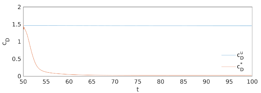
Figure 6: Drag coefficient ($c_{D}$) of the fluidic pinball over time ($t$). $c_{D}^{u}$ denotes drag of unforced flow while $c_{D}^{\star}$ represents the value for the best control.

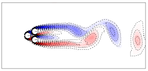
(a)

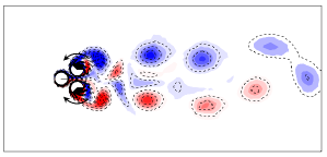
(b)

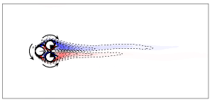
(c)

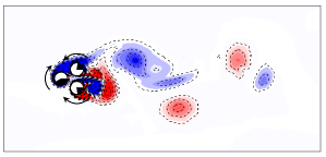
(d)

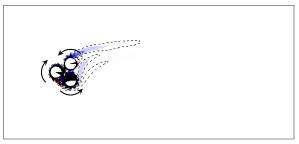
(e)

(f)

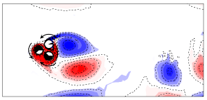
(g)

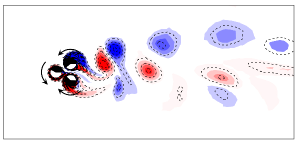
(h)

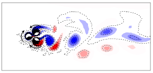
(i)

(j)

Figure 7: Fluidic pinball flows of different actuations of the control landscape (Figure 5b). Subfigure $a-j$ corresponds to actuations with letters $A$–$J$, respectively, and display the vorticity of the post-transient snapshot. Positive (negative) vorticity is color-coded in red (blue). The dashed lines correspond to iso-contourlines of vorticity. The orientation of the cylinder rotations is indicated by the arrows. The cylinder rotation is proportional to the angle of the black sector inside.

In the subsequent study, the actuation commands $b_{1}=U_{F}$, $b_{2}=U_{B}$ and $b_{3}=U_{T}$ are bounded by 5, i.e, the search space reads

$$\Omega:=\left\{[b_{1},b_{2},b_{3}]^{\rm T}\in R^{3}\colon|b_{i}|\leq 5\quad\hbox{for}\quad i=1,2,3\right\}.$$ (11)

Previous symmetric parametric studies have identified symmetric Coanda forcing $b_{1}=0$, $b_{2}=-b_{3}$ around $2$ as optimal for net drag reduction, both in low-Reynolds number direct numerical simulations (Cornejo Maceda et al., 2019) and in high-Reynolds number unsteady Reynolds Averaged Navier-Stokes (URANS) simulations (Raibaudo et al., 2019). The chosen bound of $5$ adds a large security factor to these values, i.e., the optimum can be expected to be in the chosen range. Steady bleed into the wake region is reported as another means for wake stabilization by suppressing the communication between the upper and lower shear layer. This study starts from the base-bleeding control in search of a different actuation from boat tailing.

The Latin hypercube sampling (LHS), downhill simplex method (DSM) and explorative gradient method (EGM) are applied to minimize the net drag power (8) with steady actuation in the three-dimensional domain (11). Following § 2.4 and 2.6, the initial simplex comprises four vertices: the individual controlled by base-bleeding actuation ($b_{1}=0,b_{2}=-3,b_{3}=3$), the other three individuals are positively shifted by 0.1 for each actuation. The individuals and their corresponding costs are listed in table 2. All the individuals have a larger cost than the unforced benchmark $J=1.4611$. The increase of the actuation amplitude($m=2,m=4$) indicates higher cost. And the indivudual with a smaller bottom actuation($m=3$) is associated with a smaller cost. Thus, the initial condition seems to pose a challenge for optimization.

In this section, the optimization process of EGM is investigated. Figure 5a shows the best cost found with $m$ simulation. EGM is quickly and practically converged after $m=32$ evaluations and yields the near-optimal actuation at the $95^{th}$ test

$$b^{\star}_{1}=0.1004,\quad b^{\star}_{2}=1.8645,\quad b^{\star}_{3}=-1.8314,\quad J^{\star}=0.8711.$$ (12)

The cost function $J^{\star}=0.8711$ reveals a net drag power saving of $40\%$ with respect to the unforced value $J_{u}=1.4611$. The large amount of suboptimal testing is indicative for a complex control landscape.

As displayed in figure 6, the drag coefficient falls from $1.4597$ for unforced flow to $0.0253$ for the actuation (12) within few convective time units. This near-optimal actuation corresponds to 98% drag reduction. This 98% reduction of drag power requires 58% investment in actuation energy.

The best actuation corresponds to nearly symmetric Coanda forcing with a circumferential velocity of 1.8. This actuation deflects the flow towards the positive $x$-axis and effectively removes the dead-water region with reversal flow. The slight asymmetry of the actuation is not a bug but a feature of the optimal actuation after the pitchfork bifurcation at $Re_{2}\approx 68$. This achieved performance and actuation is similar to the optimization feedback control achieved by machine learning control (Cornejo Maceda et al., 2019), comprising a slightly asymmetric Coanda actuation with small phasor control from the front cylinder. Also, the optimized experimental stabilization of the high-Reynolds number regime lead to asymmetric steady actuation (Raibaudo et al., 2019). The asymmetric forcing may be linked to the fact that the unstable asymmetric steady Navier-Stokes solutions have a lower drag than the unstable symmetric solution.

Figure 5b shows the control landscape, i.e., two-dimensional proximity map of the three-dimensional actuation parameters. Neighbouring points in the proximity map correspond similar actuation vectors. The proximity map is computed with classical multi-dimensional scaling (Cox & Cox, 2000). This map shows all performed simulations for figure 5a as solid red circles, when the evaluation improves the cost with respect to the iteration history and as open blue circles otherwise. Select new minima are highlighted with yellow circles: The first run $m=1$ on the right side, the converged run $m=95$ on the left, and the intermediate runs $m=24$ and $30$ when the explorative step jumps in new better territories. The colorbar represents interpolated values of the cost (8).

The meaning of the feature coordinates $\gamma_{1}$ and $\gamma_{2}$ will be revealed by following analysis. Ten of the individuals of the control landscape are selected and marked with letters between $A$ and $J$:

A) unforced flow

in the center;

B) base-bleeding flow

$m=1$ as the initial individual;

C) optimal actuation

after $m=95$ evaluations;

D) an asymmetric base-bleeding actuation

$m=84$ showing a strong front actuation;

E) an almost single actuation

$m=37$ at the bottom cylinder;

F–J) extreme actuations

at the boundary of the control landscape corresponding to $m=60$, $m=39$, $m=63$, $=15$, respectively.

The flows corresponding to actuations $A$–$J$ in figure 5b are depicted in figure 7. The optimized actuation ($C$) yields a partially stabilized flow, like the machine learning feedback control by Cornejo Maceda et al. (2019). Actuation $C$ corresponds to complete stabilizations with strong Coanda forcing, located near $\gamma_{2}\approx 0$ for small $\gamma_{1}$. In contrast, flow $B$ on the opposite side of the control landscapes represents strong base bleeding. Actuations $J$, $G$ and $H$, located at the top and bottom of the control landscapes correspond to Magnus effects. Large positive (negative) feature coordinates $\gamma_{2}$ are associated with large positive (negative) total circulations and associated lift forces. Summarizing, the analysis of these points reveals that the feature coordinate $\gamma_{1}$ corresponds to the strength of the Coanda forcing and is hence related to the drag. In contrast, $\gamma_{2}$ is correlated with the total circulation of the cylinder rotations and thus with the lift. Ishar et al. (2019) arrives at a similar interpretation of the proximity map for differently actuated fluidic pinball simulations.

4.3 Downhill simplex method

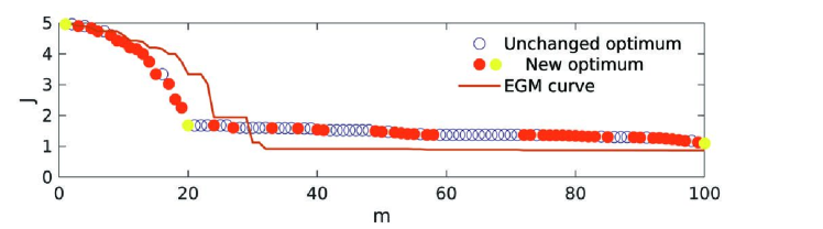
(a)

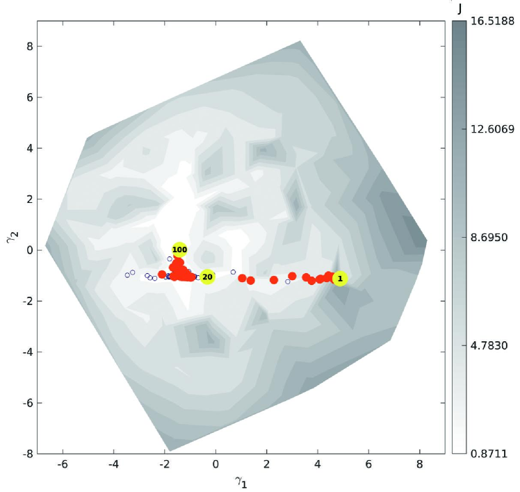
(b)

Figure 8: Same as figure 5, but with DSM.

Figure 8a shows the optimization process of the downhill simplex method (DSM). After step-by-step decends in the former 20 simulations, the net drag cost decreases slowly during the following $80\%$ computation. The optimal actuation after $100$ simulation is $b_{1}=0.1632$, $b_{2}=1.5346$, $b_{3}=-1.5378$) with cost $J=0.8937$.

Figure 8b reveals the optimization from a broad slope to a tortuous valley after the $20^{th}$ test. In face of the complex landscape on the way to global optimum (from $\gamma=[4,-1]^{\rm T}$ to $\gamma=[-1,0]^{\rm T}$), DSM consumes relatively high computation resources. EGM is seen to outperform DSM at $m\geq 30$ because of an explorative step. For random initial conditions, DSM often performs better than EGM, because the exploration as insurrance policy brings less return for this comparatively simple control landscape.

4.4 Latin hypercube sampling

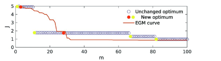
(a)

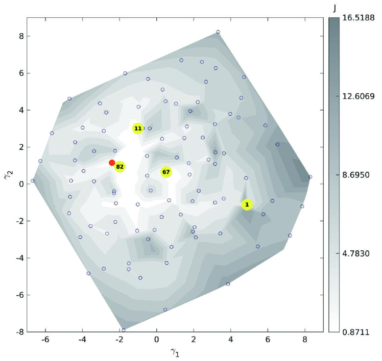
(b)

Figure 9: Same as figure 5, but with LHS.

Figure 9a shows the performance of Latin hypercube sampling (LHS). The algorithm is low-efficient during the most computation with only 4 new optima found. The jump at the $11^{th}$ DNS reduces the cost by more than $50\%$. The new optimum at $28^{th}$ simulation does not bring significant improvement, followed by a stagnation for about $40\%$ of the optimization period. The $67^{th}$ and $82^{rd}$ simulation further reduces the cost to 0.9741 with actuation $b_{1}=0.3787$, $b_{2}=2.0935$, $b_{3}=-2.0287$.

The global search is further illustrated by the uniform tested points in figure 9b. The algorithm starts near $\gamma=[4,-1]^{\rm T}$ and explore the feature space from the boundary to the central area. Three better minimum are explored one by one before the $82^{rd}$ individual near to the global mimimum is found. LHS outperforms EGM at $m=11$ before EGM leads at $m\geq 30$. Exploration is seen to have advantages at the beginning but exploitation wins already in the mid-term.

5 Drag optimization of an Ahmed body with 10 actuation parameters

Starting point of the computational fluid dynamics plant is an experimental study of a low-drag $35^{\circ}$ Ahmed body (Li et al., 2018b). The investigated Ahmed body configuration (§ 5.1) has the same physical dimensions. The effect of actuation is assessed with a Reynolds-Averaged Navier-Stokes (RANS) simulation (§ 5.2). In § 5.3, a parametric drag study with a single tangential actuator on the top edge is performed. In § 5.4, the tangential blowing of all five actuator groups is optimized for drag reduction. The explorative gradient method (EGM) is contrasted to the downhill simplex method (DSM) and Latin hypercube sampling (LHS). In § 5.5, the velocity and oriention of the five slot actuators are optimized with EGM, thus giving rise to a ten-dimensional search space. As expected drag reduction increases with the dimension of the search space, i.e., expanding actuation opportunities. The corresponding physical drag reduction mechanisms are investigated.

5.1 Configuration

Point of departure is an experimentally investigated 1:3-scaled Ahmed body characterized by a slanted edge angle of $\alpha=35^{\circ}$ with length $L$, width $W$ and height $H$ of $348\>\rm mm$, $130\>mm$ and $96\>\rm mm$, respectively. The front edges are rounded with a radius of $0.344\>H$. The model is placed on four cylindrical supports with a diameter equal to $10\>\rm mm$ and the ground clearance is $0.177\>H$. The origin of the Cartesian coordinate system $(x,y,z)$, is located in the symmetry plane on the lower edge of the model’s vertical base (see figure 10). Here, $x$, $y$ and $z$ denote the streamwise, spanwise and wall-normal coordinate, respectively. The velocity components in the $x$, $y$ and $z$ directions are denoted by $u$, $v$ and $w$, respectively. The free-stream velocity is chosen to be $U_{\infty}=30\>\rm m/s$.

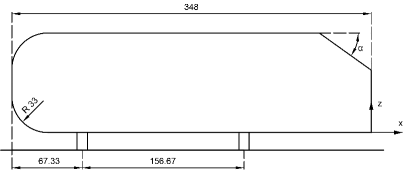
(a)

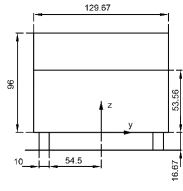
(b)

Figure 10: Dimensions of the investigated 1:3-scaled Ahmed body. a) Side view. b) Back view. The length unit is $\rm mm$ and the angle is specified in degrees.

Five groups of steadily blowing slot actuators (figure 11) are deployed on all edges of the rear window and the vertical base. All slot widths are $2\>\rm mm$. The horizontal actuators at the top, middle and bottom side have lengths of $109\>\rm mm$. The upper and lower sidewise actuators on the upper and vertical rear window have a length of $71\>mm$ and $48\>\rm mm$, respectively. The actuation velocities $U_{1},\ldots,U_{5}$ are independent parameters. $U_{1}$ refers to the upper edge of the rear window, $U_{3}$ to the middle edge and $U_{5}$ to the lower edge of the vertical base. $U_{2}$ and $U_{4}$ correspond to the velocities at the right and left sides of the upper and lower window, respectively.

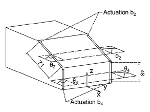
(a)

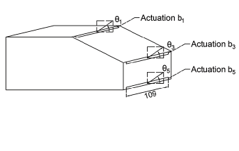
(b)

Figure 11: Deployment and blowing direction of actuators on the rear window and the vertical base. The angles $\theta_{1}$, $\theta_{2}$, $\theta_{3}$, $\theta_{4}$ and $\theta_{5}$ are all defined to be positive when pointing outward (subfigure a) or upward (subfigure b).

Following the experiment by Zhang et al. (2018), all blowing angles can be varied as indicated in figure 11. This study aims at minimizing drag as represented by the drag coefficient, $J=c_{D}$, by varying the actuation control parameters. The actuation velocity amplitudes $U_{i}$, $i=1,\ldots,5$ are capped by twice of the single optimum value as discussed in § 5.3. The actuation angles $\theta_{i}$, $i=1,\ldots,5$ are fixed to $0^{\circ}$, i.e., streamwise direction, in a 5-dimensional optimization. The actuation angles are later added into the input parameters in 10-dimensional optimization, with variable angles $\theta_{1}\in[-35^{\circ},90^{\circ}]$, $\theta_{2},\theta_{3},\theta_{4},\theta_{5}\in[-90^{\circ},90^{\circ}]$.

5.2 RANS simulation

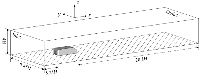
Figure 12: Computational domain of the RANS simulation.

Mesh grid points	2.5M	5M	10M
Drag Coefficient	0.294	0.313	0.318

Table 3: Drag coefficient based on different mesh resolutions.

A numerical wind tunnel (figure 12) is constructed using the commercial grid generation software Ansys ICEM CFD. The rectangular computational domain is bounded by $X_{1}\leq x\leq X_{2}$, $0\leq z\leq H_{T}$, $|y|\leq W_{T}/2$. Here, $X_{1}=-5.21\>H,X_{2}=20.17\>H$, $H_{T}=4H$, and $W_{T}=9.45H$. A coarse, medium and fine mesh using unstructured hexahedral computational grid are employed in order to evaluate the performance of RANS method for the current problem with different mesh resolutions. The statistics in Table 3 show that using a finer mesh can be expected to have negligible improvement on the accuracy of the drag coefficient. Hence, the more economical medium mesh 13 is used. This mesh consists of 5 million elements and features dimensionless wall values $\Delta x^{+}=20,\Delta y^{+}=3,\Delta z^{+}=30$. In addition to resolving the boundary layer, the shear layers and the near-wake region, the mesh near the actuation slots is also refined.

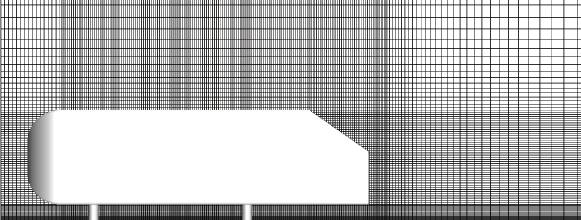
Figure 13: Side view of the part of the computational grid used for RANS.

Reynolds-Averaged Navier-Stokes (RANS) simulations using the realizable $k-\epsilon$ model with the constant parameters

$$\sigma_{k}=1.0,\sigma_{\varepsilon}=1.2,C_{2}=1.9, \quad\quad C_{1}=\max\left(0.43,\frac{\eta}{\eta+5}\right),$$

$$\eta=\left(2\sum\limits_{i,j=1}^{3}E_{ij}E_{ji}\right)^{1/2}\frac{k}{\varepsilon}, \quad\quad E_{ij}=\frac{1}{2}\left(\frac{\partial{u_{i}}}{\partial{x_{j}}}+\frac{\partial{u_{j}}}{\partial{x_{i}}}\right).$$

$\sigma_{k}=1.0$, $\sigma_{\epsilon}=1.2$, $C_{2}=1.9$ are performed employing the commercial flow solver Ansys Fluent. The spatial discretization is based on a second-order upwind scheme in the form of SIMPLE scheme based on a pressure-velocity coupling method. RANS simulation have been frequently and successfully been used to assess actuation effects from steady blowing (Ben-Hamou et al., 2007; Dejoan et al., 2005; Muralidharan et al., 2013; Viken et al., 2003). We deem RANS simulations to provide reasonable qualitative and approximately quantitative indications for actuator optimization and plan an experimental validation in the future. Partially Averaged Navier-Stokes (PANS) simulations (Han et al., 2013) and Large Eddy Simulation (LES) (Krajnović, 2009; Brunn & Nitsche, 2006) are trusted higher-fidelity simulations for drag reduction with active flow control but are computationally orders of magnitudes more demanding.

5.3 Formulation of an optimization problem based on streamwise blowing at the top edge

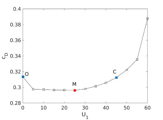
Figure 14: Drag coefficient as a function of the blowing velocity $U_{1}$ of the streamwise-oriented top actuator. Here, ‘$O$’ marks the drag without forcing, ‘$M$’ the best actuation, and ‘$C$’ the smallest actuation with worse drag than for unforced flow.

The formulation and constraints of the optimization problem is motivated by the drag reduction results from the top actuator blowing in streamwise direction. Figure 14 shows the drag coefficient in dependency of streamwise blowing velocity, all other actuators being off. The blowing velocity varies in increments of $5\>\rm m/s$ from $0\>\rm m/s$ to $60\>\rm m/s$, i.e., reaches twice the oncoming velocity.

The drag coefficient is quickly reduced by modest blowing, has a shallow minimum near the actuation velocity $U_{b1}=25\>\rm m/s$ before quickly increasing with more intense blowing. This optimal value corresponds to $5/6$ of the oncoming velocity. The best drag reduction is 5% with respect to the unforced flow $C_{d}=0.3134$. Near $U_{1}=45\>\rm m/s$, the drag rapidly rises beyond the unforced value.

This behaviour motivates the choice of actuation parameters. The first five actuation parameters are normalized jet velocities $b_{i}=U_{i}/U_{b1}$, $i=1,\ldots,5$ introduced in § 5.1. Thus, $b_{1}=1$ corresponds to minimal drag with a single streamwise-oriented top actuator. All $b_{i}$ are capped by $2$: $b_{i}\in[0,2]$, $i=1,\ldots,5$. At $b_{1}=1.8$, point ‘$C$’ in figure 14, actuation yields already drag increase. The first vertex of the amoeba of the downhill simplex search is put at $b_{1}=b_{2}=b_{3}=b_{4}=b_{5}=1.8$. From figure 14, we expect a drag minimum at lower values, hence the next five vertices test the value $1.6$, e.g. $(b_{1},b_{2},\ldots,b_{5})=\left(1.8-0.2\delta_{1,m-1},1.8-0.2\delta_{2,m-1},\ldots,1.8-0.2\delta_{5,m-1}\right)$ for $m=2,\ldots,6$. The downhill simplex algorithm may be expected to move to the outer border of the actuation domain, if maximum drag reduction lies outside the domain, thus indicating too restrictive constraints. An example is drag reduction of wall turbulence (Fernex et al., 2020).

We refrain from starting already with a much larger actuation domain, as the exploration with LHS and the proposed explorative gradient search will consistently test too many large velocities. An increase of the upper velocity bound by a factor 2, for instance, implies that only $2^{-5}$ or around 3% of uniformly distributed sampling points are in the original domain and 97% of the samples are outside.

The next five parameters characterize the deflection of the actuator velocity with respect to the streamwise direction (see § 5.1), $b_{i+5}=\theta_{i}/(\pi/2)$, $i=1\ldots,5$, and are normalized with $90^{\circ}$. Now all $b_{i}$, $i=1,\ldots,10$ span an interval of width 2, except for the more limited deflection $b_{6}$ of the top actuator. Summarizing, the domain for the most general actuation reads

$$\Omega:=\left\{\bm{b}\in{\cal R}^{10}\>\colon\>\begin{array}[]{ll}b_{i}\in[0,2]&\hbox{for }i=1,\ldots,5\\ b_{i}\in\left[-35/90,1\right]&\hbox{for }i=6\\ b_{i}\in[-1,1]&\hbox{for }i=7,\ldots,10\end{array}\right\}.$$ (13)

The choice of $\bm{b}$ as symbol shall remind about the control $B$-matrix in control theory and is consistent with many earlier publications of the authors, e.g., the review article by Brunton & Noack (2015).

5.4 Optimization of the streamwise trailing edge actuation

The drag of the Ahmed body is optimized with streamwise blowing from the five slot actuators. We apply a simplex downhill search, Latin hypercube sampling and the explorative gradient method of § 5.4.1, § 5.4.2 and § 5.4.3, respectively.

5.4.1 Downhill simplex algorithm

$m$	$b_{1}$	$b_{2}$	$b_{3}$	$b_{4}$	$b_{5}$	J
1	1.8	1.8	1.8	1.8	1.8	0.4153
2	1.6	1.8	1.8	1.8	1.8	0.4048
3	1.8	1.6	1.8	1.8	1.8	0.4109
4	1.8	1.8	1.6	1.8	1.8	0.3996
5	1.8	1.8	1.8	1.6	1.8	0.4075
6	1.8	1.8	1.8	1.8	1.6	0.4040

Table 4: Initial simplex ($m=1,\ldots,6$) for the five-dimensional downhill simplex optimization. $b_{i}$ are the normalized actuation velocities and $J$ corresponds to the drag coefficient.

Following § 5.3, the downhill simplex algorithm is centered around $b_{i}=1.8$, $i=1,\ldots,5$ as first vertex and explores a lower actuation $b_{m-1}=1.6$ in all directions for vertices $m=2,\ldots,6$. Table 4 shows the values of the individuals and corresponding cost. All vertices have a larger drag than for the unforced benchmark $C_{d}=0.3134$. And all vertices with $b_{i}=1.6$ are associated with a smaller drag indicating a downhill slide to small actuation values consistent with the expectations from § 5.3.

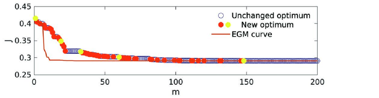
(a)

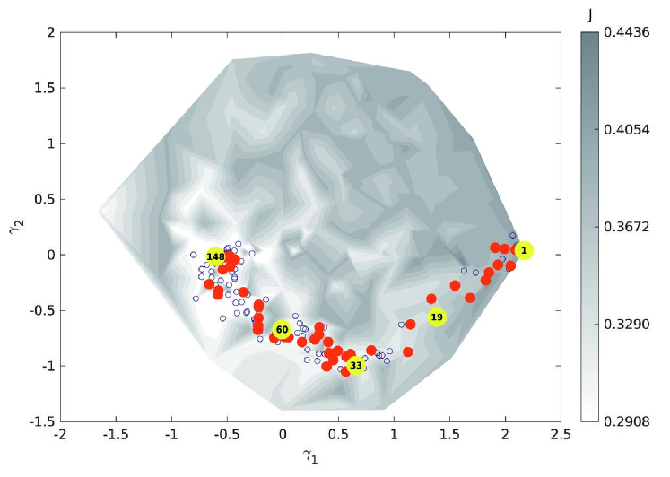
(b)

Figure 15: Optimization of five tangential jet actuator groups with DSM. The top figure displays the best achieved drag reduction in terms of the number of evaluations (RANS simulations). The bottom figure shows the proximity map of all evaluated actuations. The contour plot corresponds to the interpolated cost function (drag coefficient) from all RANS simulations of this section. As in § 3, solid red circles mark newly find optima while open blue circles mark unsuccessful tests of cost functions. For better interpretability, select newly found optima are highlighted with by a yellow solid circle like in § 4. In the control landscape, these circles are marked with the index $m$.

Figure 15 (top) shows the evolution of the downhill simplex algorithm with 200 RANS simulations. Like in § 3, solid red circles mark newly found optima while open blue circles record the best actuation so far. The drag quickly descends after staying shortly on a plateau at $m\approx 20$. From there on, the descent becomes gradual. The optimal drag $J=0.2908$ is reached with the 148th RANS simulation and corresponds to 7% drag reduction. The optimal actuation reads $b_{1}=0.7264$, $b_{2}=0.5508$, $b_{3}=0.1533$, $b_{4}=0.6746$, $b_{5}=0.7716$. While the middle horizontal jet has small amplitude, the other actuation velocities on the four edges of the Ahmed body are $55$% to $77$% of the optimal value achieved with single actuator.

Figure 15 (bottom) illustrates the downhill search in a control landscape $J(\gamma_{1},\gamma_{2})$ described in § 2. Here $(\gamma_{1},\gamma_{2})$ feature vectors defining a proximity map of the five-dimensional actuation parameters $(b_{1},\ldots,b_{5})$. This landscape indicates a complex topology of the five-dimensional actuation space by many local maxima and minima in the feature plane. This complexity may explain why most simplex steps did not yield a better cost. The feature coordinate $\gamma_{1},\gamma_{2}$ arise from a kinematic optimization process and have no inherent meaning. The simplex algorithm is seen to crawl from right $\bm{\gamma}\approx(2,0)$ to the assumingly global minimum at $\bm{\gamma}\approx[-0.6,0]^{\rm T}$ through an elongated curved valley. The simulation results for $m=1$, $19$, $33$, $60$ and $148$ are marked with yellow solid circles. Note that the construction of this proximity map includes also undisplayed actuation data from LHS and EGM so that the control landscapes remain identical for all discussed five-dimensional actuations.

5.4.2 Latin hypercube sampling

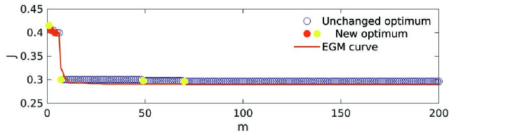
(a)

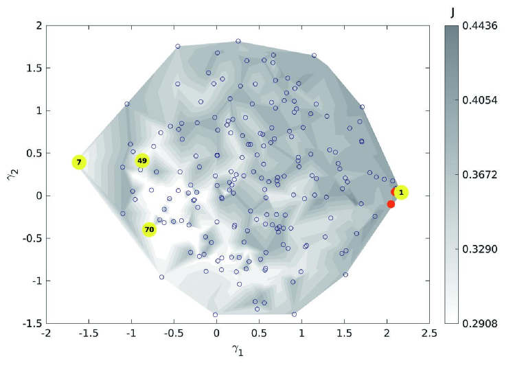
(b)

Figure 16: Same as figure 15, but with LHS.

Figure 16 (top) shows the slow learning process associated with Latin hypercube sampling (LHS) starting with the simplex reference point $b_{1}=\ldots=b_{5}=1.8$. Apparently the optimization is ineffective. Only 3 new optima are successively obtained in 200 RANS simulations. The remaining simulations yield worse drags than the best discovered before. At the 70th RANS simulation, the best drag coefficient of $C_{d}=0.2928$, with $b_{1}=0.0994$, $b_{2}=0.9587$, $b_{3}=0.1276$, $b_{4}=0.0289$ and $b_{5}=1.0393$. corresponds to 5% reduction like the one-dimensional top actuator $b_{1}=1$, $b_{2}=b_{3}=b_{4}=b_{5}=0$. Intriguingly, only the upper side and bottom actuator have $b_{i}$ amplitudes near unity while remaining parameters are less than 13% of the one-dimensional optimum. These results show that near optimal drag reductions can be achieved with quite different actuations. Moreover, individual actuation effects are far from additive. Otherwise, the almost complimentary LHS optimum for actuators 2–5 and the one-dimensional optimum of § 5.3 should yield 10% reduction with $b_{1}\approx 1$, $b_{2}\approx 1$, $b_{3}\approx 0.13$, $b_{4}\approx 1$ and $b_{5}\approx 1$.

Figure 16 (bottom) shows the LHS in the control landscape. In the first iteration, LHS jumps to the opposite site of domain and finds better drag. The next successive two improvements are in a good terrain but the optimum at $m=70$ is still far from the assumingly global minimum at $\bm{\gamma}\approx(-0.6,0)$ (see figure 15). The exploratory steps uniformly cover the whole range of feature vectors.

5.4.3 Explorative gradient method

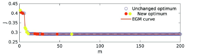
(a)

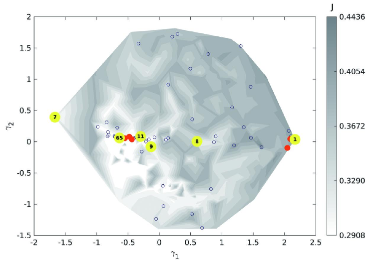
(b)

Figure 17: Same as figure 15, but with EGM.

From the figure 17, the explorative gradient method is seen to converge much faster than the downhill simplex algorithm. The best actuation is found at the 65th RANS simulation yielding the same drag coefficient $C_{d}=0.2908$ of the downhill simplex algorithm with only slightly different actuation parameters $b_{1}=0.6647$, $b_{2}=0.4929$, $b_{3}=0.1794$, $b_{4}=0.7467$ and $b_{5}=0.7101$.

The fast convergence of the explorative gradient method is initially surprising since up to 50% of the steps are for explorative purposes, i.e., shall identify distant minima. However, the control landscape in figure 16 reveals how the explorative LHS steps help the algorithm to prevent the long and painful march through the long and curved valley. At $m=7$, an explorative step leads to the opposite side of control landscape with a better cost value. Then, the subsequent iterations quickly lead near global minimum at $m=11$. The proposed new algorithm operates like a visionary mountain climber, who performs not only local uphill steps but sends drones to the remotest location to find better mountains and terrains.

5.5 Optimization of the directed trailing edge actuation

In this section, the actuation space is enlarged by the jet directions of all slot actuators. The jets may now be directed inwards or outwards as discussed in § 5.1. The actuation optimization for drag reduction is performed with explorative gradient method (§ 5.5.1). The unforced and three actuated Ahmed body wakes are investigated in § 5.5.2.

5.5.1 Explorative gradient method

We employ the explorative gradient method as best performing method of § 5.4 for the 10-dimensional actuation optimization problem. The search is accelerated by starting with a simplex centered around the optimal actuation of the five-dimensional problem. The first vertex of table 5 contains this optimal solution. The cost is $4\permil$ lower than the previous section as the RANS integration for the first flow is not fully converged. The next five vertices represent isolated actuations at the optimal value but directed $45^{\circ}$ outwards for the side edges and upwards for the middle horizontal actuator. The corresponding drag values are larger. The next five vertices deflect the jets in opposite direction by $45^{\circ}$ or the maximum $35^{\circ}$ of the top actuator, giving rise smaller drag than the previous deflection. The drag of middle horizontal actuator remains close to the unforced benchmark because the jet velocity is small.

$m$	$b_{1}$	$b_{2}$	$b_{3}$	$b_{4}$	$b_{5}$	$b_{6}$	$b_{7}$	$b_{8}$	$b_{9}$	$b_{10}$	$J$
1	0.6647	0.4929	0.1794	0.7467	0.7101	0	0	0	0	0	0.2895
2	0.6647	0	0	0	0	1/2	0	0	0	0	0.3268
3	0	0.4929	0	0	0	0	1/2	0	0	0	0.3226
4	0	0	0.1794	0	0	0	0	1/2	0	0	0.3168
5	0	0	0	0.7467	0	0	0	0	1/2	0	0.3476
6	0	0	0	0	0.7101	0	0	0	0	1/2	0.3060
7	0.6647	0	0	0	0	-35/90	0	0	0	0	0.3091
8	0	0.4929	0	0	0	0	-1/2	0	0	0	0.3085
9	0	0	0.1794	0	0	0	0	-1/2	0	0	0.3187
10	0	0	0	0.7467	0	0	0	0	-1/2	0	0.3001
11	0	0	0	0	0.7101	0	0	0	0	-1/2	0.3354

Table 5: Initial individuals in the optimization of the directed trailing edge actuation. $b_{i}$, $i=1,2,3,4,5$ represent the actuation amplitudes $U_{i}$ of the $i$th actuator. $b_{i}$, $i=6,7,8,9,10$ denotes the actuation angle $\theta_{i}$ of the $(i-5)$th actuator. $J$ is the drag coefficient.

Figure 18 (top) illustrates the convergence of the explorative gradient method. After 289 RANS simulations, a drag coefficient of $0.2586$ is achieved corresponding to a 17% drag reduction. The optimal actuation values read $b_{1}=0.8611$, $b_{2}=0.9856$, $b_{3}=0.0726$, $b_{4}=1.0089$, $b_{5}=0.8981$, $b_{6}=-0.3000$ corresponding to $\theta_{1}=-27^{\circ}$, $b_{7}=-0.4666$ ($\theta_{2}=-42^{\circ}$), $b_{8}=0.7444$ ($\theta_{3}=67^{\circ}$), $b_{9}=-0.4888$ ($\theta_{3}=-44^{\circ}$), and $b_{10}=0.2444$ ($\theta_{3}=-22^{\circ}$). All outer actuators have velocity amplitudes near unity and are directed inwards, i.e., emulate Coanda blowing. The third middle actuator blows upward with low amplitude. The strong inward blowing seems to be related to the additional 10% drag reduction as compared to the 7% of streamwise actuation.

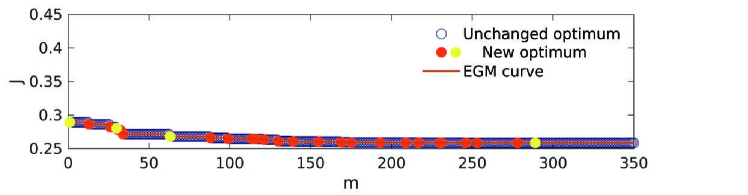
(a)

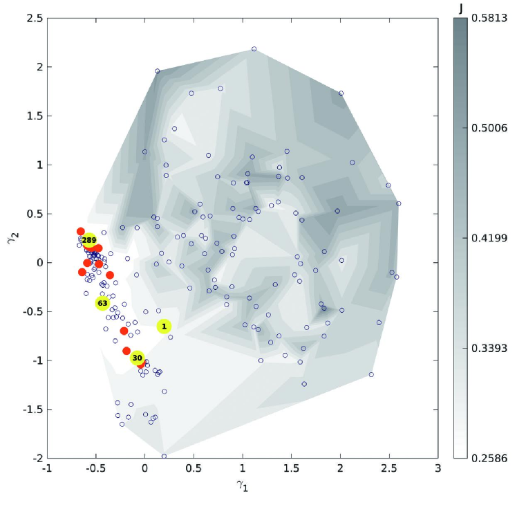
(b)

Figure 18: Same as figure 17, but for the 10-dimensional optimization of the orientable trailing edge actuation with EGM.

Figure 18 (bottom) shows the search process in a proximity map. It should be noted that this control landscape is based on data in a ten-dimensional actuation space and hence different from the 5-dimensional space in § 5.4. The algorithm quickly descends in the valley while many exploration steps probe suboptimal terrain. One reason for this quick landing in good terrain is the chosen initial simplex around the optimized actuation in the five-dimensional subspace.

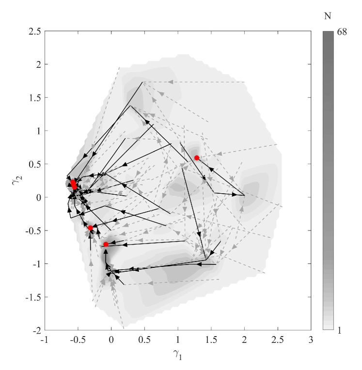
Figure 19: Steepest decent lines of the control landscape depicted in figure 18. For details see text.

The topology of the control landscape of figure 18 is investiged with discrete steepst descent lines connecting neighboring data points in figure 19. For each investigated actuation vector, the nearest five neighbours are considered. If all neighbours have higher drag, the vector is considered as a local minimum and marked by a red point. Otherwise, a gray dashed arrow is plotted to the best of these neighbour. This steepest descent is continued until a local minimum is reached. The corresponding path is called (discrete) steepest descent line. Line segments shared by at least 10 of these pathes may be considered as important valleys towards the minimum and highlighted as black solid arrow. The visiting times of each individual are marked by colorcoding. The global minimum of all data points is visited most, 54 steepest descend lines end here. The resulting pathways of ‘mountain trails’ to ‘expressways’ may give an indication of the directions to be expected from local search algorithms. Moreover, crossing steepest descent lines indicate that the two-dimensional proximity maps oversimplifies a higher-dimesional landscape structure. Intriguingly, the steepest descent line become more aligned to each other in the valleys leading to global data minimum, i.e., the most relevant regions for optimization.

5.5.2 Discussion of streamwise and directed jet actuators

In the following, the physical structures associated with the optimized one-, five- and ten-dimensional actuation are discussed. Evidently, more degrees of freedom are associated with more opportunities for drag reduction. Expectedly, the drag reduces by 5% to 7% to 17% as the dimension of the actuation parameters increase from 1 to 5 to 10, respectively. Intriguingly, the increase of drag reduction from the optimized top actuator to the best 5 streamwise actuators is only 2%. For the square-back Ahmed body, Barros (2015) experimentally observed that the individual drag reductions from the streamwise blowing actuators on the four trailing edges roughly add up to the total drag reduction of 10% with all actuators on. This additivity of actuation effects is not corroborated for the slanted low-drag Ahmed body. Intriguingly, the inward deflection of the jet-slot actuators substantially decreases drag by 10%. This additional drag reduction of 10% has also been observed for the square-back Ahmed body when the horizontal jets were deflected inward with Coanda surfaces on all four edges (Barros et al., 2016). Improved drag reduction with inward as opposed to tangential blowing was also observed for the $35^{\circ}$ high-drag Ahmed body (Zhang et al., 2018) and the square back version Schmidt et al. (2015).

Table 6 summarizes the discussed flows, associated drag reduction and actuation parameters. For brevity, we refer to flows with no, one-dimensional, five-dimensional and ten-dimensional actuation spaces as case A, B, C and D, respectively. The actuation energy may be conservatively estimated by the energy flux through all jet actuators: $\sum_{i=1}^{5}\int d\!A_{i}\rho U_{i}^{3}/2$. Here, the actuation jet fluid is assumed to be accelerated from $0$ to the actuation jet velocity $U_{i}$ and then deflected after the outlet, e.g., via a Coanda surface. In this case, the actuation energy of cases $B$, $C$ and $D$ would correspond to $3.2\%$, $3.0\%$ and $7.9\%$ of the parasitic drag power, respectively. This expenditure is significantly less than the saved drag power. The ratio from saved drag power to actuation energy is comparable for a truck model where steady Coanda blowing with 7% energy expenditure yields a 25% drag reduction (Pfeiffer & King, 2014). This estimate should not be taken too literally as actuation energy strongly depends on the realization of the actuator. It would be less, more precisely $\sum_{i=1}^{5}\int d\!A_{i}\>\rho\cos(\theta_{i})\>U_{i}^{3}/2$, when the actuation jet fluid leaves the Ahmed body through a slot directed with the jet velocity, and can be expected much less when this fluid is taken from the oncoming flow, e.g., from the front of the Ahmed body.

Case	Drag reduction	Actuation parameters
		Top	Upper side	Middle	Lower side	Bottom
A)	$0\%$	—	—	—	—	—
B)	$5\%$	$b_{1}=1$	$b_{2}=0$	$b_{3}=0$	$b_{4}=0$	$b_{5}=0$
C)	$7\%$	$b_{1}=0.6647$	$b_{2}=0.4929$	$b_{3}=0.1794$	$b_{4}=0.7467$	$b_{5}=0.7101$
D)	$17\%$	$b_{1}=0.8611$	$b_{2}=0.9856$	$b_{3}=0.0726$	$b_{4}=1.0089$	$b_{5}=0.8981$
		$\theta_{1}=-27^{\circ}$	$\theta_{2}=-42^{\circ}$	$\theta_{3}=67^{\circ}$	$\theta_{3}=-44^{\circ}$	$\theta_{3}=-22^{\circ}$

Table 6: Investigated optimized actuations in comparison to the unforced benchmark. The table shows the achieved drag reduction and corresponding actuation parameters for A) the unforced benchmark, and for the optimized B) top streamwise actuator, C) all streamwise actuators, D) all deflected actuators.

Figure 20 displays iso-surfaces for the same Okubo-Weiss parameter value $Q$ for all four cases. The unforced case A (figure 20a) shows a pronounced C-pillar vortices extending far into the wake. Under streamwise top actuation (case B, figure 20b), the C-pillar vortices significantly shorten. The next change with all streamwise actuators optimized (case C) is modest consistent with the small additional drag decrease. The C-pillar vortices are slightly more shortened (see figure 20c). The inward deflection of the actuation (case D) is associated with aerodynamic boat tailing as displayed in figure 20d. The separation from the slanted window is significantly delayed and the sidewise separation is vectored inward.

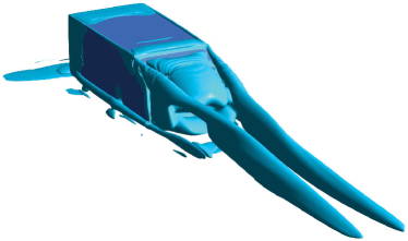
(a)

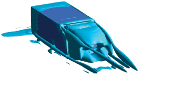
(b)

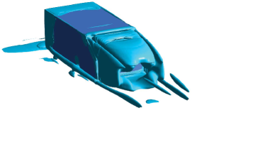
(c)

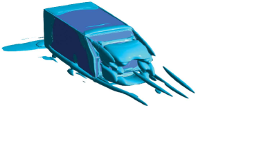
(d)

Figure 20: Okubo-Weiss parameter $Q$ of flow. a) without control and under b) 1D, c) 5D and d) 10D control respectively, where $Q=15000/s^{2}$.

This actuation effect on the C-pillar vortices is corroborated by the streamwise vorticity contours in a transverse plane on body height downstream ($x/H=1$). Figure 21 shows this averaged vorticity component for case A–D in subfigure a–d, respectively. The extension of the C-pillar vortices clearly shrink with increasing drag reduction.

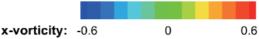
(a)

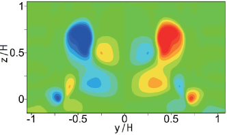
(a)

(b)

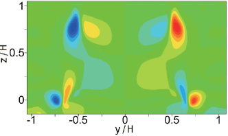
(c)

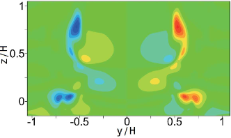
(d)

Figure 21: Streamwise vorticity component in near-wake plane $x/H=1$. a) without forcing and under b) 1D, c) 5D and d) 10D control respectively.

Figure 22 shows the streamwise velocity component and streamlines of the transversal velocity in the same plane for the same cases. Cases B and C feature a larger region of upstream flow while case D has a narrowed region of backflow. From these visualizations, one may speculate that the drag reduction from streamwise actuation (cases B and C) is due to a wake elongation towards the Kirchhoff solution while the inward directed actuation (case D) is associated with drag reduction from aerodynamic boat-tailing.

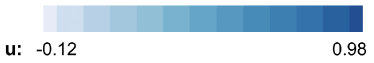
(a)

(a)

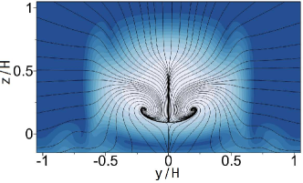
(b)

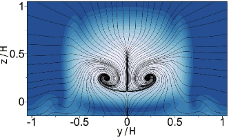
(c)

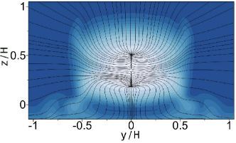
(d)

Figure 22: Streamwise velocity component in the near-wake tranversal plane $x/H=1$ and streamlines from the in-plane velocity components. a) without forcing and under b) 1D, c) 5D and d) 10D control respectively.

This hypothesis about different mechanisms of drag reduction is corroborated from the streamlines in the symmetry plane $y=0$ in figure 23. The tangential blowing (see subfigures b, c leads to an elongated fuller wake as compared to the unforced benchmark (subfigure a). The top shear-layer is oriented more horizontal under streamwise actuation—consistent with the Kirchhoff wake solution. The inward-directed actuation (see subfigure d) also elongates the wake but gives rise to a more streamlined shape. The top and bottom shear-layers are vectored inward.

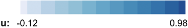
(a)

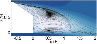
(a)

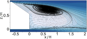
(b)

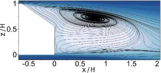
(c)

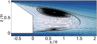
(d)

Figure 23: Streamwise velocity component in the symmetry plane $y=0$ and streamlines from the in-plane velocity components. a) without forcing and under b) 1D, c) 5D and d) 10D control respectively.

The drag reduction can more directly be inferred from the $C_{p}$ distribution of the rearward windows in figure 24. The 5% drag reduction in subfigure b) for case B is associated with a pressure increase of the vertical surface. The additional 2% drag decrease for case C in subfigure c is accompanied by an increase over vertical and slanted surface. The aerodynamic boat-tailing of case D with 17% drag reduction alleviates significantly the pressures on both surfaces.

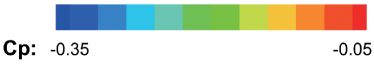
(a)

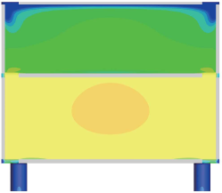
(a)

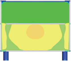
(b)

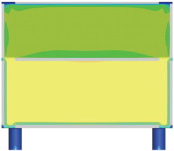
(c)

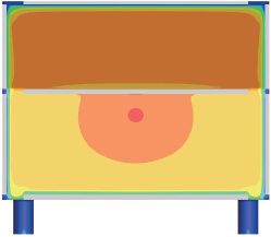
(d)

Figure 24: Pressure coefficient on the slant and vertical base of flow. a) without forcing and under b) 1D, c) 5D and d) 10D control respectively.

6 Conclusions

We propose a novel optimization approach for active bluff-body control exploiting local gradients with a downhill simplex algorithm and exploring new better minima with Latin hypercube sampling (LHS). This approach is called explorative gradient method (EGM) as the iterations alternate between downhill simplex iteration as a robust gradient method and LHS as the most explorative step. A distinguishing feature of EGM is that it performs an ‘aggressive’ exploitation in one step and the arguably most optimal exploration in another step. Thus, both, exploitation and exploration come with optimizing principles and with an a priori evaluation investment which is determined upfront. This policy has distinct advantages. In some cases, the exploitation will be pointless because the best minimum still needs to be found. In other cases, the exploration will be ineffective, because the dimension or complexity of the search space is too large. EGM hedges against both scenarios of inefficiency because high-dimensional search spaces typically have unknown characteristics.

This policy may be contrasted with genetic algorithms which can be remarkably effective in high dimensions, but the goal of explorative operations, like mutation, and exploitative operations, like crossover, come with no optimizing principle, like gradient-based convergence or geometric coverage of the search space. A similar observation applies to other biologically inspired optimization methods (see, e.g., Wahde, 2008), like ant colony or particle swarm optimization. As another example, simulated annealing explores good minima before it increasingly exploits them. Here, again, exploration and exploitation come with no optimizing principle and the switch between exploration and exploitation is a design parameter. We argue that the radical alternation between gradient-based exploitation and maximal exploration is one of the most promising strategies in an unknown search space.

EGM is compared with other optimizers for an analytical test function with one global and for local minima. The study includes the failure rate in finding the global optimum and the convergence rate. EGM is found to be distinctly superior in both aspects in comparison with (1) Latin hypercube sampling (LHS), (2) Monte Carlo sampling, (3) a genetic algorithm, (4) a downhill simplex method, and (5) a random restart or shotgun downhill optimization. This behaviour is made physically plausible for smooth cost functions with few mininima, i.e., a typical case for active flow control.

As first flow control example, EGM is applied to the minimization of the parasitic net drag power of the multi-input fluidic pinball problem. It yields a slightly asymmetric Coanda forcing with 40 % net drag power reduction comprising 98 % drag reduction penalized by 58 % actuation energy. As very similar actuation has been found with machine learning control for feedback law ansatz (Cornejo Maceda et al., 2019). This Coanda actuation foreshadows the optimization result of the subsequent drag minimization of the Ahmed body. Intriguingly, EGM also probed base bleed and circulation control as options for drag power minimization.

EGM reduces the drag of a $35^{\circ}$ slanted Ahmed body by 17% with independent steady blowing at all trailing edges at Reynolds number $Re_{H}=1.9\times 10^{5}$. The 10-dimensional actuation space includes 5 symmetric jet slot actuators or corresponding actuator groups with variable velocity and variable blowing angle. The resulting drag is computed with a Reynolds-Averaged Navier-Stokes (RANS) simulation.

The approach is augmented by auxiliary methods for initial conditions, for accelerated learning and for a control landscape visualization. The initial condition for a RANS simulation with a new actuation is computed by the 1-nearest neighbour method. In other words, the RANS simulation starts with the converged RANS flow of the closest hitherto examined actuation. This cuts the computational cost by 60% as it accelerates RANS convergence. The actuation velocities are quantized to prevent testing of too similar control laws. This optional element reduces the CPU time by roughly 30%. The learning process is illustrated in a control landscape. This landscape depicts the drag in a proximity map—a two-dimensional feature space from the high-dimensional actuation response. Thus, the complexity of the optimization problem can be assessed.

The slanted Ahmed body with 1, 5 and 10 actuation parameters constitutes a more realistic plant for an optimization algorithm. First, only the upper streamwise jet actuator is optimized. This yields drag reduction of 5% with pronounced global minimum for the jet velocity. Second, the drag can be further reduced to 7% with 5 independent streamwise symmetric actuation jets. Intriguingly, the actuation effects of the actuator are far from additive—contrary to the experimental observation for the square-back Ahmed body (Barros, 2015). The optimal parameters of a single actuator are not closely indicative for the optimal values of the combined actuator groups. The control landscape depicts a long curved valley with small gradient leading to a single global minimum. Interestingly, the explorative step is not only a security policy for the right minimum. It also helps to accelerate the optimization algorithm by jumping out of the valley to a point closer to the minimum.

A significant further drag reduction of 17% is achieved when, in addition to the jet velocities, also the jet angles are included in the optimization. Intriguingly, all trailing edge jets are deflected inward mimicking the effect of Coanda blowing and leading to fluidic boat tailing. The C-pillar vortices are increasingly weakened with one-, five- and ten-dimensional actuation. Compared with the pressure increase at C-pillar in one- and five-dimensional control, the ten-dimensional control brings a substantial pressure recovery over the entire base. The achieved 17% drag decrease with constant blowing is comparable with the experimental 20% reduction with high-frequency forcing by Bideaux et al. (2011); Gilliéron & Kourta (2013).

For the $25^{\circ}$ high-drag Ahmed body, (Zhang et al., 2018) have achieved 29% drag reduction with steady blowing at all sides, thus significantly outperforming all hitherto existing active flow control studies cited therein. The actuation has only been investigated for few selected actuation values. Hence, even better drag reductions are perceivable. Yet, the unforced high-drag Ahmed body has a significantly higher drag coefficient of $0.361$ than the low-drag version and is hence not fully comparable. Their reduced drag coefficient of $0.256$ is almost identical with the one of this study.

We expect that our RANS-based active control optimization is widely applicable for virtually all multi-input steady actuations or combinations of passive and active control (Bruneau et al., 2010). The explorative gradient method mitigates the chances of sliding down a suboptimal minimum at an acceptable cost. The 1-nearest neighbour method for initial condition and the actuation quantization accelerate the simulations and learning processes. And the control landscape provides the topology of the actuation performance, e.g., the number of local minima, nature and shape of valleys, etc.

The current performance benefits of EGM over other commonly used optimizers has also been corroborated in preliminary bluff-body drag reduction experiments in Europe and China. Evidently, the optimizer can also be employed for cost function minimization for design parameters of passive devices or parameters of closed-loop control schemes. An exciting new avenue is the generalization of EGM from a parameter optimizer to a regression problem solver: EGM has recently been applied to optimize multi-input multi-output control laws for the stabilization of the fluidic pinball and was found to be distinctly superior to genetic programming (Cornejo Maceda et al., 2020).

The key idea of EGM is to balance exploration and exploitation by aiming to optimizing each for one step in an alternating fashion. If the dimension of the search space is too large, the downhill simplex algorithm may be replaced by a subplex (King & Rowan, 2020) or a stochastic gradient method. Similarly, for large dimensions, the LHS may need to be replaced by Monte Carlo sampling or a genetic algorithm. Note that LHS will first explore the edge of the search space before it explores the center.

Summarizing, EGM is a versatile optimizer framework with numerous future applications. The very algorithms of EGM cannot only be applied to parameter optimization but also to model-free control law optimization, hitherto performed by genetic programming (Gautier et al., 2015; Ren et al., 2020) and deep reinforcement learning (Rabault et al., 2019; Bucci et al., 2019). Preliminary results for the fluidic pinball indicate that the learning rate increases by one order of magnitude as compared to linear genetic programming control (Li et al., 2018a). Future versions of EGM will also incorporate the learning of response models with methods of machine learning (see, e.g., Brunton & Kutz, 2019) for accelerate learning.

Declaration of interests

The authors report no conflict of interest.

Appendix A Genetic algorithm

This section provides further details about the chosen matlab realization of the genetic algorithm.

1) First generation.

The algorithm begins by creating an initial population with random inviduals. Each parameter of each individual is taken with uniform probability from a given interval.

2) Next generations.

The algorithm uses the individuals in the current generation, called parents, to create individuals of the next population, called children:

a) Cost evaluation.

Score each member of the current population by computing its cost function. The cost function is assumed to be sorted, $J_{1}\leq J_{2}\leq\ldots\leq J_{r}\leq\ldots J_{I}$. The index is called the rank.

b) Scaled fitness.

Scale the cost function based on relative ordering. An individual with rank $r$ has fitness score of $1/\sqrt{r}$ (higher fitness, smaller rank).

c) Parents.

Select members, called parents, based on their expectation value. The selection function chooses parents for the next generation based on their expectation values. An individual can be selected more than once as a parent, in which case it contributes its genes to more than one child.

d) Elitism.

The best $N_{e}$ individuals are copied directly into the new generation. This number corresponds to the probability $P_{e}=0.05$, i.e., $N_{e}=I*P_{e}$

e) Mutation and crossover.

Produce children from the parents with crossover or mutation. By combining parts of genes from a pair of parents, crossover children are produced with probability $P_{c}=0.8$. The remaining individuals, other than elite children, are mutation children by making random changes to a single parent. Scattered, the default crossover function, creates a random binary vector and selects the genes where the vector is a 1 from the first parent, and the genes where the vector is a 0 from the second parent, and combines the genes to form the child. The default mutation function—Gaussian adds a random number taken from a Gaussian distribution with mean 0 to each entry of the parent vector. The standard deviation of this distribution is determined by the parameters Scale 1 and Shrink 1.(Matlab 2018b)

f) Next generation.

This generation comprises all children as created above.

3) Termination.

The algorithm stops when a stopping criter is met. Here, the stopping criteria is the maximum generation number $L$.

References

- Aider et al. (2010) Aider, J.-L., Beaudoin, J.-F. & Wesfreid, J. E. 2010 Drag and lift reduction of a 3D bluff-body using active vortex generators. Exp. Fluids 48, 771–789.
- Barros (2015) Barros, D. 2015 Wake and drag manipulation of a bluff body using fluidic forcing. PhD thesis, École Nationale Supérieure de Mécanique et d’Aérotechnique, Poitiers, France.
- Barros et al. (2016) Barros, D., Borée, J., Noack, B. R., Spohn, A. & Ruiz, T. 2016 Bluff body drag manipulation using pulsed jets and Coanda effect. J. Fluid Mech. 805, 442–459.
- Ben-Hamou et al. (2007) Ben-Hamou, E., Arad, E. & Seifert, A. 2007 Generic transport aft-body drag reduction using active flow control. Flow Turbul. Combust. 78 (3-4), 365.
- Bideaux et al. (2011) Bideaux, E., Bobillier, P., Fournier, E., Gilliéron, P., El Hajem, M., Champagne, J.-Y., Gilotte, P. & Kourta, A. 2011 Drag reduction by pulsed jets on strongly unstructured wake: towards the square back control. Int. J. Aerodyn. 1 (3-4), 282–298.
- Bruneau et al. (2010) Bruneau, C.-H., Creusé, E., Depeyras, D., Gilliéron, P. & Mortazavi, I. 2010 Coupling active and passive techniques to control the flow past the square back Ahmed body. Comput. & Fluids 39 (10), 1875–1892.
- Brunn & Nitsche (2006) Brunn, A & Nitsche, W 2006 Drag reduction of an ahmed car model by means of active separation control at the rear vehicle slant. In New Results in Numerical and Experimental Fluid Mechanics V, pp. 249–256. Springer.
- Brunton & Kutz (2019) Brunton, S. L. & Kutz, N. 2019 Data-Driven Science and Engineering. Cambridge University Press.
- Brunton & Noack (2015) Brunton, S. L. & Noack, B. R. 2015 Closed-loop turbulence control: Progress and challenges. Appl. Mech. Rev. 67 (5), 050801:01–48.
- Bucci et al. (2019) Bucci, M. A., Semeraro, O., Allauzen, A., Wisniewski, G., Cordier, L. & Mathelin, L. 2019 Control of chaotic systems by deep reinforcement learning. Proc. Roy. Soc. London A 475, 20190351.
- Chen et al. (2020) Chen, W., Ji, C., Alam, Md M., Williams, J. & Xu, D. 2020 Numerical simulations of flow past three circular cylinders in equilateral-triangular arrangements. Journal of Fluid Mechanics 891, 1–44.
- Cornejo Maceda et al. (2020) Cornejo Maceda, G. Y., Li, Y., Lusseyran, F., Morzyński, M. & Noack, B. R. 2020 Stabilization of the fluidic pinball with gradient-based machine learning control. J. Fluid Mech. (in preparation), 1–44.
- Cornejo Maceda et al. (2019) Cornejo Maceda, G. Y., R., Noack B., Lusseyran, F., Deng, N., Pastur, L. & Morzyński, M. 2019 Artificial intelligence control applied to drag reduction of the fluidic pinball. Proc. Appl. Math. Mech. 19 (1), e201900268:1–2.
- Cox & Cox (2000) Cox, T. F. & Cox, M. A. A. 2000 Multidimensional Scaling, 2nd edn., Monographs on Statistics and Applied Probability, vol. 88. Chapman and Hall.
- Dejoan et al. (2005) Dejoan, A, Jang, Y. J. & Leschziner, M. A. 2005 Comparative LES and unsteady RANS computations for a periodically-perturbed separated flow over a backward-facing step. J. Fluids Eng. 127 (5), 872–878.
- Deng et al. (2020) Deng, N., Noack, B. R., Morzyński, M. & Pastur, L. R. 2020 Low-order model for successive bifurcations of the fluidic pinball. J. Fluid Mech. 884, A37.
- Fernex et al. (2020) Fernex, D., Semann, R., Albers, M., Meysonnat, P. S, Schröder, W. & Noack, B. R. 2020 Self-similar drag reduction formula from sparse data—Optimization of turbulent skin-friction via spanwise travelling surface waves. Phys. Rev. Fluids 5 (7), 073901:1–18.
- Gautier et al. (2015) Gautier, N., Aider, J.-L., Duriez, T., Noack, B. R., Segond, M. & Abel, M. W. 2015 Closed-loop separation control using machine learning. J. Fluid Mech. 770, 424–441.
- Geropp (1995) Geropp, D. 1995 Process and device for reducing the drag in the rear region of a vehicle, for example, a road or rail vehicle or the like. United States Patent US 5407245 A.
- Geropp & Odenthal (2000) Geropp, D. & Odenthal, H.-J. 2000 Drag reduction of motor vehicles by active flow control using the Coanda effect. Exp. Fluids 28 (1), 74–85.
- Gilliéron & Kourta (2013) Gilliéron, P. & Kourta, A. 2013 Aerodynamic drag control by pulsed jets on simplified car geometry. Exp. Fluids 54 (2), 1457.
- Glezer et al. (2005) Glezer, A., Amitay, M. & Honohan, A.M. 2005 Aspects of low- and high-frequency actuation for aerodynamic flow control. AIAA Journal 43 (7), 1501–1511.
- Gad-el Hak (2006) Gad-el Hak, M. 2006 Flow Control: Passive, Active, and Reactive Flow Management. Cambridge university press.
- Han et al. (2013) Han, X., Krajnović, S. & Basara, B. 2013 Study of active flow control for a simplified vehicle model using the PANS method. Int. J. Heat Fluid Flow 42, 139–150.
- Hucho (2002) Hucho, W.-H. 2002 Aerodynamik der stumpfen Körper. Physikalische Grundlagen und Anwendungen in der Praxis, 2nd edn. Wiesbaden: Vieweg Verlag.
- Humphrey & Wilson (2000) Humphrey, D. G. & Wilson, J. R. 2000 A revised simplex search procedure for stochastic simulation response surface optimization. INFORMS Journal on Computing 12 (4), 272–283.
- Ishar et al. (2019) Ishar, R., Kaiser, E., Morzynski, M., Albers, M., Meysonnat, P., Schröder, W. & Noack, B. R. 2019 Metric for attractor overlap. J. Fluid Mech. 874, 720–752.
- Kim (2011) Kim, J. 2011 Physics and control of wall turbulence for drag reduction. Phil. Trans. Roy. Soc. A 369 (1940), 1396–1411.
- King & Rowan (2020) King, A. A. & Rowan, T. 2020 Subplex: Unconstrained optimization using the subplex algorithm.
- Krajnović (2009) Krajnović, S. 2009 Large eddy simulation of flows around ground vehicles and other bluff bodies. Phil. Trans. R. Soc. A 367 (1899), 2917–2930.
- Li et al. (2018a) Li, R., Noack, B. R., Cordier, L., Borée, J., Kaiser, E. & Harambat, F. 2018a Linear genetic programming control for strongly nonlinear dynamics with frequency crosstalk. Archives of Mechanics 70 (6), 505–534.
- Li et al. (2018b) Li, Y., Cui, W., Jia, Q. & Yang, Z. 2018b Wake control on a simplified vehicle using steady blowing. In Proceedings of the 8th International Conference on Fluid Mechanics (ICFM8), pp. 1–6. Paper.
- McKay et al. (1979) McKay, M. D., Beckman, R. J. & Conover, W. J. 1979 Comparison of three methods for selecting values of input variables in the analysis of output from a computer code. Technometrics 21 (2), 239–245.
- Minelli et al. (2020) Minelli, G., Dong, T., Noack, B. R. & Krajnović, S. 2020 Upstream actuation for bluff-body wake control driven by a genetically inspired optimization. J. Fluid Mech. 893, A1.
- Muralidharan et al. (2013) Muralidharan, K, Muddada, S. & Patnaik, B. S. V. 2013 Numerical simulation of vortex induced vibrations and its control by suction and blowing. Appl. Math. Model. 37 (1-2), 284–307.
- Nelder & Mead (1965) Nelder, J. A. & Mead, R. 1965 A simplex method for function minimization. J. Comput. 7, 308–313.
- Park et al. (2006) Park, H., Lee, D., Jeon, W.-P., Hahn, S., Kim, J., Choi, J. & Choi, H. 2006 Drag reduction in flow over a two-dimensional bluff body with a blunt trailing edge using a new passive device. J. Fluid Mech. 563, 389–414.
- Pastoor et al. (2008) Pastoor, M., Henning, L., Noack, B. R., King, R. & Tadmor, G. 2008 Feedback shear layer control for bluff body drag reduction. J. Fluid Mech. 608, 161–196.
- Pfeiffer & King (2014) Pfeiffer, J. & King, R. 2014 Linear parameter varying active flow control for a 3d bluff body exposed to cross-wind gusts. In AIAA Paper, 2014-2406.
- Press et al. (2007) Press, W.H., Flamery, B.P., Teukolsky, S.A. & Vetterling, W.T. 2007 Numerical Recipes, The Art of Scientific Computing, 3rd edn. Cambridge, UK, etc.: Cambridge University Press.
- Protas (2004) Protas, B. 2004 Linear feedback stabilization of laminar vortex shedding based on a point vortex model. Phys. Fluids 16 (12), 4473–4488.
- Rabault et al. (2019) Rabault, J., Kuchta, M., Jensen, A., Réglade, U. & Cerardi, N. 2019 Artificial neural networks trained through deep reinforcement learning discover control strategies for active flow control. J. Fluid Mech. 865, 281–302.
- Raibaudo et al. (2019) Raibaudo, C., Zhong, P., Noack, B. R. & Martinuzzi, R. J. 2019 Machine learning strategies applied to the control of a fluidic pinball. Phys. Fluids 32, 015108.
- Ren et al. (2020) Ren, F., Hu, H.-B. & Tang, H. 2020 Active flow control using machine learning: A brief review. J. Hydrodyn. 32 ((2)), 247–253.
- Schmidt et al. (2015) Schmidt, H.-J., Woszidlo, R., Nayeri, C. N. & Paschereit, C. O. 2015 The effect of flow control on the wake dynamics of a rectangular bluff body in ground proximity. Exp. Fluids 56, 151.
- Thiria et al. (2006) Thiria, B., Goujon-Durand, S. & Wesfreid, J. E. 2006 The wake of a cylinder performing rotary oscillations. J. Fluid Mech. 560, 123–147.
- Viken et al. (2003) Viken, S., Vatsa, V., Rumsey, C. & Carpenter, M. 2003 Flow control analysis on the hump model with RANS tools. In 41st Aerospace Sciences Meeting and Exhibit, p. 218.
- Wahde (2008) Wahde, M. 2008 Biologically Inspired Optimization Methods: An Introduction. WIT Press.
- Wood (1964) Wood, C. J. 1964 The effect of base bleed on a periodic wake. Journal of the Royal Aeronautical Society 68 (643), 477–482.
- Wright (1991) Wright, Alden H 1991 Genetic algorithms for real parameter optimization. In Foundations of genetic algorithms, , vol. 1, pp. 205–218. Elsevier.
- Zhang et al. (2018) Zhang, B. F., Liu, K., Zhou, Y., To, S. & Tu, J. Y. 2018 Active drag reduction of a high-drag Ahmed body based on steady blowing. J. Fluid Mech. 856, 351––396.